


1. Introduction
Due to their low drag coefficients, slender bodies are used extensively in aerospace and naval applications. Multiple studies have described the flow around these bodies, focusing on the drag force, the boundary layer and the flow separation (Wang Reference Wang1970; Costis, Telionis & Hoang Reference Costis, Telionis and Hoang1989; Wang et al. Reference Wang, Zhou, Hu and Harrington1990; Chesnakas & Simpson Reference Chesnakas and Simpson1994; Fu et al. Reference Fu, Shekarriz, Katz and Huang1994; Constantinescu et al. Reference Constantinescu, Pasinato, Wang, Forsythe and Squires2002; Wikström et al. Reference Wikström, Svennberg, Alin and Fureby2004). However, despite their presence in many underwater applications, only a few works have looked into the wake of a slender body (Chevray Reference Chevray1968; Jiménez, Hultmark & Smits Reference Jiménez, Hultmark and Smits2010; Kumar & Mahesh Reference Kumar and Mahesh2018), and the far wake of a slender body has been studied only recently (Ortiz-Tarin, Nidhan & Sarkar Reference Ortiz-Tarin, Nidhan and Sarkar2021).
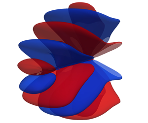
The near wake of a slender body with a turbulent boundary layer (TBL) is characterized by having a small recirculation region. The recirculation region is surrounded by a ring of small-scale turbulence that emerges from the boundary layer and does not show strong vortex shedding (Jiménez et al. Reference Jiménez, Hultmark and Smits2010; Posa & Balaras Reference Posa and Balaras2016; Kumar & Mahesh Reference Kumar and Mahesh2018; Ortiz-Tarin et al. Reference Ortiz-Tarin, Nidhan and Sarkar2021). As a result, the wake is thin and develops slowly compared with the wake of a bluff body. These particular features of the slender-body high- ${Re}$ near wake lead to interesting effects further downstream: (i) despite having a smaller drag coefficient than bluff bodies, the defect velocity (
 $U_d=U_\infty -U$) of the slender-body wake can be larger than that of a bluff body for a long downstream distance; (ii) the turbulent kinetic energy of the wake shows an off-centre radial peak at the location where the TBL separates – instead of a Gaussian profile with a central peak; and (iii) helical instabilities come into play only in the intermediate and far field of the wake. These particularities affect the scaling laws of the wake. In a domain spanning
  $80D$, the defect velocity, the kinetic energy and the dissipation do not follow the classic high-
 ${Re}$ scaling and they decay differently than bluff-body wakes (Ortiz-Tarin et al. Reference Ortiz-Tarin, Nidhan and Sarkar2021), exhibiting a non-equilibrium scaling of dissipation (Dairay, Obligado & Vassilicos Reference Dairay, Obligado and Vassilicos2015; Vassilicos Reference Vassilicos2015).
The few studies that look into slender-body wakes assume that the body moves in an unstratified environment, where the density of the surrounding fluid is constant. However, in a realistic underwater marine environment, the effect of density stratification due to salinity and temperature can become relevant. Density stratification suppresses vertical motions, triggers the formation and sustenance of coherent structures, and leads to the radiation of internal gravity waves. More importantly, in a stratified environment, the wake of a submersible lives longer than in an unstratified environment, i.e. it takes more time for the flow disturbance to die out (Spedding Reference Spedding2014). The study of stratified wakes has been nearly exclusively focused on the flow past bluff bodies (Lin & Pao Reference Lin and Pao1979; Hanazaki Reference Hanazaki1988; Chomaz et al. Reference Chomaz, Bonneton, Butet, Perrier and Hopfinger1992; Lin et al. Reference Lin, Lindberg, Boyer and Fernando1992; Orr et al. Reference Orr, Domaradzki, Spedding and Constantinescu2015; Pal et al. Reference Pal, Sarkar, Posa and Balaras2017) and underwater topography (Drazin Reference Drazin1961; Castro, Snyder & Marsh Reference Castro, Snyder and Marsh1983; Baines Reference Baines1998). Here, we study the influence of stratification on the high- ${Re}$ wake of a prolate spheroid with a TBL.
The strength of ambient stratification is measured by the body-based Froude number  ${Fr}=U_\infty /ND$. This is the ratio between the convective frequency of the flow,
  $U_\infty /D$ – where
  $U_\infty$ is the freestream velocity, and
  $D$ is the diameter of the body – and the buoyancy frequency
  $N$. In the wake of ocean submersibles,
  ${Fr} \sim O(1 {--}10^2)$. However, since the velocity deficit in the wake
  $U_d(x)$ decays with the streamwise distance, and the wake width
  $L(x)$ increases, the Froude number defined with local variables
  ${Fr}_l=U_d/NL$ decreases as the flow evolves. Thus even in a weakly stratified environment, eventually all wakes are affected by stratification.
Since the relative strength of stratification increases locally as the flow develops, the evolution of the stratified wake is multistage in nature. Based on the measurements of  $U_d$ and
  $L$ in high-
 ${Fr}$ (i.e. initially weak stratification) bluff-body wakes, Spedding (Reference Spedding1997) identified three regimes in stratified wake evolution based on the power-law decay rates of
  $U_d$. These regimes are generally identified by empirically fitting decay rates to
  $U_d$ in different temporal (or spatial) regions and are as follows.
(i) Three-dimensional (3-D) regime. Close to the generator, wake decay is similar to the unstratified wake of the corresponding body shape. This is the so-called 3-D regime and lasts until the buoyancy time defined by
 $Nt = Nx/U = (x/D)(1/{Fr})$ approaches $O(1)$, equivalently until $x/D \sim {Fr}$.
(ii) Non-equilibrium (NEQ) regime. As the wake evolves, buoyancy effects become progressively stronger. The decay of
$U_d$ slows relative to the 3-D regime, and furthermore, anisotropy between the vertical and horizontal velocity components increases. Spedding (Reference Spedding1997) reported this NEQ region to last for $Nt \approx 2 {--}50$. Later, temporal simulations of Brucker & Sarkar (Reference Brucker and Sarkar2010) and Diamessis, Spedding & Domaradzki (Reference Diamessis, Spedding and Domaradzki2011) found an increase in the span of the NEQ regime at higher Reynolds numbers. According to Spedding (Reference Spedding1997), $U_d \sim x^{-0.25 \pm 0.04}$ during the NEQ regime. However, there has been some variability in the observed NEQ decay rate in later studies. Bonnier & Eiff (Reference Bonnier and Eiff2002) reported an NEQ regime with $U_d \sim x^{-0.38}$ for $1.5 < {Fr} < 5$. Brucker & Sarkar (Reference Brucker and Sarkar2010) and Diamessis et al. (Reference Diamessis, Spedding and Domaradzki2011) reported $U_d \sim Nt^{-1/4}$ during the NEQ regime in their temporal simulations. Chongsiripinyo & Sarkar (Reference Chongsiripinyo and Sarkar2020) found that $U_d \sim x^{-0.18}$ during the NEQ regime of their ${Fr} = 2$ and $10$ disk wakes. For wakes with ${Fr} \sim O(1)$, the NEQ decay rate is preceded by a pronounced oscillatory modulation in $U_d$ that is linked to lee waves (Pal et al. Reference Pal, Sarkar, Posa and Balaras2017; Ortiz-Tarin, Chongsiripinyo & Sarkar Reference Ortiz-Tarin, Chongsiripinyo and Sarkar2019; Chongsiripinyo & Sarkar Reference Chongsiripinyo and Sarkar2020).(iii) Quasi-two-dimensional (Q2D) regime. After the NEQ regime, the stratified wake enters into the Q2D regime, which is characterized by transition in the
$U_d$ power law to a significantly increased decay rate; e.g. Spedding (Reference Spedding1997) reports a transition to $U_d \sim x^{-3/4}$. In the Q2D regime, the wake organizes progressively into vortices that meander primarily in the horizontal plane (Gourlay et al. Reference Gourlay, Arendt, Fritts and Werne2001; Dommermuth et al. Reference Dommermuth, Rottman, Innis and Novikov2002; Brucker & Sarkar Reference Brucker and Sarkar2010) and take the form of ‘pancakes’. Although the wake motion in this regime is primarily in the horizontal plane, there is a variability in the vertical direction in the form of layers (Spedding Reference Spedding2002), hence the prefix ‘quasi’.


In recent literature, stratified wakes have been characterized using turbulence features (Zhou & Diamessis Reference Zhou and Diamessis2019; Chongsiripinyo & Sarkar Reference Chongsiripinyo and Sarkar2020) instead of the  $U_d$-based criteria of Spedding (Reference Spedding1997). These studies are motivated by an attempt to connect buoyancy-related wake transitions to the broader stratified turbulence field.
Notice that the arrival of the wake into each of the three stages in its evolution depends on the value of  $Nt$, which is equivalent to a downstream distance
  $x/{Fr}$ from the wake generator. At high Froude number, the downstream distance required to reach the NEQ and Q2D regions can become very large. Consequently, the size of the computational domain required to access these regimes rapidly becomes computationally unfeasible. To circumvent these limitations, temporal simulations were used in the study of Gourlay et al. (Reference Gourlay, Arendt, Fritts and Werne2001). Temporal simulations use a reference frame moving with the wake, where time correlates with streamwise distance in a fixed reference frame. By assuming that the streamwise development of the flow is slow, periodic boundary conditions can be used and the equations are advanced in time without the need to introduce the wake generator. This reduces the computational cost significantly. Most of the studies that have contributed to our current understanding of stratified wakes use temporal simulations (Gourlay et al. Reference Gourlay, Arendt, Fritts and Werne2001; Dommermuth et al. Reference Dommermuth, Rottman, Innis and Novikov2002; Brucker & Sarkar Reference Brucker and Sarkar2010; Diamessis et al. Reference Diamessis, Spedding and Domaradzki2011; De Stadler et al. Reference De Stadler, Sarkar and Brucker2010; De Stadler & Sarkar Reference De Stadler and Sarkar2012; Abdilghanie & Diamessis Reference Abdilghanie and Diamessis2013; Redford, Lund & Coleman Reference Redford, Lund and Coleman2015; Rowe, Diamessis & Zhou Reference Rowe, Diamessis and Zhou2020).
The main drawback of the temporal model is the influence of its initialization. Since the flow at the wake generator is not solved, the starting profiles of the mean and turbulence have to be assumed. These simulations lack some specific features that are generated due to the body, e.g. steady lee waves, near-wake buoyancy effects, and the vortical structures shed from the boundary layer. Even when it is tempting to assume that body-specific features are lost far from the body, the universality of the wake decay has remained elusive to experiments (Bevilaqua & Lykoudis Reference Bevilaqua and Lykoudis1978; Wygnanski, Champagne & Marasli Reference Wygnanski, Champagne and Marasli1986; Redford, Castro & Coleman Reference Redford, Castro and Coleman2012), even in unstratified wakes. An alternative to temporal simulations are body inclusive simulations that retain the wake-generator-dependent features at the expense of a higher computational cost and a limited domain size (Orr et al. Reference Orr, Domaradzki, Spedding and Constantinescu2015; Chongsiripinyo, Pal & Sarkar Reference Chongsiripinyo, Pal and Sarkar2017; Pal et al. Reference Pal, Sarkar, Posa and Balaras2017; Nidhan et al. Reference Nidhan, Ortiz-Tarin, Chongsiripinyo, Sarkar and Schmid2019; More et al. Reference More, Ardekani, Brandt and Ardekani2021).
To the best of the authors’ knowledge, Ortiz-Tarin et al. (Reference Ortiz-Tarin, Chongsiripinyo and Sarkar2019) performed the first study of a stratified flow past a slender body that investigates the near and intermediate wake dynamics. Their analyses reveal that at  ${Fr}\sim O(1)$, the type of separation and the subsequent wake establishment are strongly dependent on the characteristic frequency of the lee waves and the aspect ratio of the body. When half the wavelength of the steady lee waves (
 $\lambda =2{\rm \pi} {Fr}$) matches the length of the slender body (
 $L$), the separation of the boundary layer is inhibited by buoyancy effects. Based on this condition, a critical Froude number can be defined
  ${Fr}_c=L/D{\rm \pi}$. When
  ${Fr}>{Fr}_c$, stratification suppresses the generation of turbulence in the near wake; when
  ${Fr}\approx {Fr}_c$, buoyancy strongly limits the flow separation and can lead to a relaminarization of the wake at low Reynolds numbers. Finally, when
  ${Fr}<{Fr}_c$, the lee waves enlarge the separation region and there might be an increase in the turbulence intensities in the wake. When
  ${Fr}\approx {Fr}_c$, the wake is in a resonant state, with both the separation and the wake dimensions being strongly modulated by the steady lee waves (Hunt & Snyder Reference Hunt and Snyder1980; Chomaz, Bonneton & Hopfinger Reference Chomaz, Bonneton and Hopfinger1993; Ortiz-Tarin et al. Reference Ortiz-Tarin, Chongsiripinyo and Sarkar2019).
As mentioned before, the use of body-inclusive simulations has one major limitation, i.e. the high computational cost. Due to the high resolution required to solve the boundary layer of the wake generator, the downstream domain is limited and thus the possibility of looking into the far wake gets significantly restricted, particularly at high  ${Re}$. VanDine, Chongsiripinyo & Sarkar (Reference VanDine, Chongsiripinyo and Sarkar2018) presented a hybrid spatially evolving model, which builds on the hybrid temporally evolving model of Pasquetti (Reference Pasquetti2011), and addresses most of the aforementioned problems. The hybrid method uses inflow conditions generated from a well-resolved body-inclusive simulation to perform a separate temporal simulation in the case of Pasquetti (Reference Pasquetti2011), or spatially evolving simulation in the work of VanDine et al. (Reference VanDine, Chongsiripinyo and Sarkar2018) without including the body. By doing so, the amount of required points is substantially reduced since the flow near the body does not have to be resolved. This important reduction of the computational cost allows one to extend the domain farther downstream to gain insight in the far wake.
Here, we use a hybrid method that combines a body-inclusive simulation and a spatially evolving body-exclusive simulation to study the stratified high- ${Re}$ far wake of a slender body for the first time. The Reynolds number is set to
  ${Re}=U_\infty D/\nu =10^5$, and two levels of stratification are used,
  ${Fr}= U_\infty /ND = 2$ and
  $10$. The simulation at
  ${Fr}=10$ allows us to study the evolution of a weakly stratified wake in a domain that spans
  $80D$. In addition,
  ${Fr}=2$ is chosen because it is close to the critical Froude number for a 6 : 1 prolate spheroid,
  ${Fr}_c= (L/D)/{\rm \pi} = 6/{\rm \pi}$. At the critical Froude number, the size of the separation region is strongly reduced by the lee waves (Ortiz-Tarin et al. Reference Ortiz-Tarin, Chongsiripinyo and Sarkar2019). These choices also allow us to compare our results with the findings of Chongsiripinyo & Sarkar (Reference Chongsiripinyo and Sarkar2020) (hereafter referred to as CS20) regarding the stratified wake of a disk.
In CS20, the stratified wake of a disk at  ${Re}=5 \times 10^4$ is studied at
  ${Fr}={2,10,50,\infty }$. Apart from a detailed analysis of the decay rates of the mean and turbulent quantities, CS20 links the general evolution of stratified homogeneous turbulence (Brethouwer et al. Reference Brethouwer, Billant, Lindborg and Chomaz2007; de Bruyn Kops & Riley Reference de Bruyn Kops and Riley2019) with the evolution of the wake turbulence. As the disk wake evolves, the influence of buoyancy is ‘felt’ by the turbulent motions at progressively smaller scales. First the mean flow and the large scales, and later the root mean square (r.m.s.) velocities, are affected by stratification. Simultaneously, the horizontal eddies start gaining energy. Based on the strength of these effects, three distinct stages can be identified: weakly, intermediate and strongly stratified turbulence. In CS20, the transition between these regimes is examined and parametrized using local Froude and Reynolds numbers. Zhou & Diamessis (Reference Zhou and Diamessis2019) also examined these transitions and their link with the evolution of stratified homogeneous turbulence using temporal simulations.
The present work is the continuation of Ortiz-Tarin et al. (Reference Ortiz-Tarin, Nidhan and Sarkar2021) – referred to as ONS21 – where the unstratified wake of a 6 : 1 prolate spheroid with a TBL was studied and compared with a large number of simulations and experiments. In our previous study, we found that the particularities of the slender-body wake – e.g. small recirculation region, low entrainment, large defect velocity, bimodal distribution of the turbulent kinetic energy – affect the wake decay significantly. In this study, we are analysing how these features affect the evolution of the stratified wake. We also analyse the simulations of CS20 to closely compare our results with the stratified bluff-body wake.
Some of the questions that we want to answer are the following. Do the stratified decay laws and their transition points depend on the shape of the wake generator? How does the turbulence evolve in stratified slender-body wakes, and are there difference with bluff-body wakes? How does the phase-space evolution of the stratified turbulence compares between bluff- and slender-body wakes? In broader terms, we attempt to find whether a turbulent stratified wake retains some imprint of the wake generator in the mean and turbulence evolution.
A description of the solver and the methodology is given in § 2. The wakes are visualized in § 3. The decay of the mean wake properties is analysed in § 4. Finally, the evolution of the turbulence and the phase-space analysis of the wake are presented in §§ 5 and 6, respectively. The study is concluded in § 7.
2. Methodology
To study the far wake of a slender body at a high Reynolds number, we use a hybrid simulation. The hybrid model combines two simulations: body-inclusive (BI), which solves the flow past the wake generator, and body-exclusive (BE), which resolves the intermediate and far wakes. Here, we use a spatially evolving simulation following the procedure validated by VanDine et al. (Reference VanDine, Chongsiripinyo and Sarkar2018). In the implementation, data from a selected cross-plane in the BI simulation are interpolated onto a new grid and used as an inlet boundary condition for the BE stage. This procedure allows us to alleviate the natural stiffness of the wake problem. Whereas the BI simulation is designed to capture the TBL and the flow separation, the BE simulation resolves the turbulence in the wake. Both the grid size and the time step required to solve the TBL are much smaller than those needed in the intermediate and far wakes. This method leads to significant savings in computational cost without compromising accuracy.
The set-up and the solver here are the ones used in ONS21 with the addition of stratification. Both simulations solve the 3-D Navier–Stokes equations with the Boussinesq approximation in cylindrical coordinates. The solver uses a third-order Runge–Kutta method combined with a second-order Crank–Nicolson method to advance the equations in time. Second-order-accurate central differences are used for the spatial derivatives in a staggered grid. A wall-adapting local eddy (WALE) viscosity is used to properly capture the TBL dynamics (Nicoud & Ducros Reference Nicoud and Ducros1999). Both the BI and BE simulations use Dirichlet boundary conditions at the inflow, convective outflow and Neumann boundary conditions at the radial boundary. Similar to Ortiz-Tarin et al. (Reference Ortiz-Tarin, Chongsiripinyo and Sarkar2019), a sponge layer is added to the boundaries to avoid the spurious reflection of gravity waves.
An immersed boundary method (Balaras Reference Balaras2004; Yang & Balaras Reference Yang and Balaras2006) is used to resolve the flow past a 6 : 1 prolate spheroid at zero angle of attack. The immersed boundary method solver has been used extensively for stratified wake simulations (Ortiz-Tarin et al. Reference Ortiz-Tarin, Chongsiripinyo and Sarkar2019; Puthan et al. Reference Puthan, Jalali, Ortiz-Tarin, Chongsiripinyo, Pawlak and Sarkar2020; CS20). A numerical bump is introduced on the surface of the body to accelerate the transition of the boundary layer to turbulence. The annular bump is located where the surface favourable pressure gradient is nearly zero. This location is found at approximately  $0.5 D$ from the nose. The radial extent of the bump is
  $0.002 D$ (
 $\sim$15 wall units), and the streamwise extent is
  $0.1 D$.
The stratification is set by a linear background density profile characterized by the Froude number  ${Fr} = U_\infty /ND$, where
  $N$ is the buoyancy frequency. Three levels of stratification are simulated:
  ${Fr}=2$,
  $10$ and
  $\infty$. Of these,
  ${Fr}=2$ is close to the critical Froude number
  ${Fr}_c = 6/{\rm \pi}$ for the 6 : 1 spheroid at which the suppression of turbulence in the wake by stratification is optimal (Ortiz-Tarin et al. Reference Ortiz-Tarin, Chongsiripinyo and Sarkar2019), whereas
  ${Fr}=10$ is a moderate level of stratification closer to oceanic values. Finally,
  ${Fr}=\infty$ is the unstratified case, which will be used as a reference (ONS21).
The cylindrical coordinate system is  $(x,r,\theta )$, with the origin at the body centre. For convenience, the Cartesian coordinate system
  $(x,y,z)$ will also be used, where
  $z$ is the vertical direction aligned with gravity,
  $y$ is the spanwise direction, and
  $x$ is the streamwise direction.
The BI grid is designed to resolve the TBL and the small-scale wake turbulence. The TBL is resolved with  $\Delta x^+=40$,
  $\Delta r^+=1$, and
  $r\,\Delta \theta ^+=32$. There are 10 points in the viscous sublayer, and 130 across the buffer and log layers. The mean velocities and turbulence intensities within the boundary layer were validated against existing studies (Posa & Balaras Reference Posa and Balaras2016; Kumar & Mahesh Reference Kumar and Mahesh2018) and the law of the wall. In addition, a grid refinement study was performed to guarantee the independence of the statistics to the grid choice.
In the wake, the peak ratio between the grid size and the Kolmogorov length  $\eta = (\nu ^3/\varepsilon)^{1/4}$, in both BI and BE domains, is
  $\max (\Delta x/\eta )=7.5$,
  $\max (\Delta r/\eta )=6$ and
 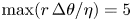 $\max (r\,\Delta \theta /\eta )=5$. Figure 2 of ONS21 shows the ratio between the Kolmogorov scale and the grid resolution. In addition, the unstratified wake decay coincides with all the previous existing numerical and experimental works on slender-body wakes (see figure 1 of ONS21).
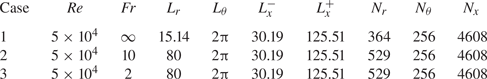
The domain size in the stratified cases is large, so internal gravity waves are weak before reaching the sponge region near the walls. The total number of grid points across BI and BE domains is approximately 1.5 billion in the unstratified case, and 2 billion in the stratified simulations. Tables 1 and 2 include the most relevant parameters of BI and BE simulations, respectively. Further details on the grid design can be found in § 2 of ONS21.
Table 1. Parameters of the BI simulation of a prolate 6 : 1 spheroid, where  $L_x^-$ and
  $L_x^+$ are the upstream and downstream distances from the wake generator.

Table 2. Parameters of the BE simulations, where  $x_{e}$ is the extraction location of the BI simulations that is fed as inlet to the BE simulations.

Once the flow has reached statistically steady state, the statistics are obtained by temporal averaging, denoted by  $\langle \cdot \rangle$. Instantaneous quantities are written with lower-case letters, mean quantities with upper-case letters, and fluctuations with primes. In the stratified cases, the average is performed over
  $270D/U_\infty$, approximately three flow-throughs. In the unstratified simulation flow, statistics are obtained through temporal (over
  $100D/U_\infty$) as well as azimuthal averaging. Apart from temporal averaging, some statistics are obtained from cross-wake area integration denoted by
  $\{ \cdot \}$. Unless otherwise indicated, the integral is performed over a cross-section of radius
  $4D$. All the flow statistics presented here die out well before they reach the limit of the integrated region.
Reported velocities and lengths are normalized with the freestream velocity  $U_\infty$ and the body minor axis
  $D$, respectively. The normalized streamwise distance from the centre of the body
  $x$ is also measured as a function of the buoyancy frequency and the time. The time in the
  $Nt$ axis refers to time measured by an observer attached to the mean flow that sees the body move at speed
  $-U_\infty$. A Galilean transformation yields
  $x/{Fr}=Nt$.
To compare the stratified wake of the 6 : 1 spheroid with that of a bluff body, we use the BI disk wake simulations of CS20. The solver used in CS20 is the same as that used here, although instead of using the WALE closure model, CS20 uses a variant of dynamic Smagorinsky. The eddy viscosity model was changed in the spheroid simulations since WALE was demonstrated to capture the behaviour of the TBL with the resolution used in the present wall-resolved large eddy simulation. Both sets of simulations are very well resolved and have a small subgrid contribution – see ONS21 and CS20 – hence the validity of the comparison. Further details of the simulations can be found in ONS21 and CS20. The main parameters of disk simulations are listed in table 3.
Table 3. Parameters of the disk simulations (CS20).
3. Visualizations
Figure 1 shows instantaneous snapshots of the near wake of a spheroid and a disk at  ${Fr} = 2$ and
  $10$. At both
  ${Fr}$ values, the near-wake structures of the two bodies are very different. Compared with the spheroid with TBL, the disk wake has a large recirculation region (
 ${\sim }2D$), as shown by the red isolines in figure 1. This large recirculation region oscillates (Rigas et al. Reference Rigas, Oxlade, Morgans and Morrison2014) and generates a vortex-shedding structure that is advected downstream (Nidhan et al. Reference Nidhan, Chongsiripinyo, Schmidt and Sarkar2020). In a spheroid with TBL, the recirculation region is very small (
 ${\sim }0.1D$) and is surrounded by the small-scale turbulence of the boundary layer. As a result, the near wake is highly organized and large-scale oscillations are not observed in the near wake (Jiménez et al. Reference Jiménez, Hultmark and Smits2010; Kumar & Mahesh Reference Kumar and Mahesh2018; ONS21). Only further downstream does the wake begin to show a helical structure. This change in the structure of the slender-body wake has been found to lead to a change in the decay rate and dissipation scaling in the unstratified wake (ONS21). In the following sections, we will analyse how the differences between the near wake of a disk and that of a spheroid lead to distinct trends of mean and turbulence evolution in a stratified environment. But first, let us describe different snapshots of the spheroid intermediate and far wakes. Snapshots of the disk intermediate and far wakes can be found in CS20.

Figure 1. Instantaneous contours of streamwise velocity in the near wake for (a,c,e,g) spheroid wakes and (b,d,f,h) disk wakes, at  ${Fr} = 2$ and
  $10$ on centre-vertical (
 $y=0$) and centre-horizontal (
 $z=0$) planes. Red isolines show the limit of recirculation regions where the streamwise velocity is zero.
Figure 2 shows an instantaneous visualization of the spheroid  ${Fr}=2$ wake in the centre-vertical and centre-horizontal planes. One of the distinctive features of the spheroid wake is that at
  ${Fr}\sim O(1)$, the separation of the boundary layer can be strongly modulated by the steady lee waves (Ortiz-Tarin et al. Reference Ortiz-Tarin, Chongsiripinyo and Sarkar2019). This interaction between the lee waves and the wake is particularly strong when the Froude number is close to a critical Froude number
  ${Fr}_c=AR/{\rm \pi}$, where
  $AR$ is the body aspect ratio. When
  ${Fr}\approx {Fr}_c$, half the wavelength of the lee wave (
 $\lambda /D=2{\rm \pi} {Fr}$) coincides with the length of the body, and the size of the separation region is reduced. The flow is then in what is called the resonant or saturated lee wave regime (Hanazaki Reference Hanazaki1988; Chomaz et al. Reference Chomaz, Bonneton, Butet, Perrier and Hopfinger1992). At low Reynolds numbers, this effect can lead to the relaminarization of the turbulent wake (Pal et al. Reference Pal, Sarkar, Posa and Balaras2016; Ortiz-Tarin et al. Reference Ortiz-Tarin, Chongsiripinyo and Sarkar2019). In the present case, figure 2(a) reveals that even at
  ${Re}=10^5$, the wake height is strongly modulated by the waves, although the wake is not relaminarized due to the high
  ${Re}$ of the flow. For example, the wake height exhibits oscillations with wavelength
  $\lambda /D= 2{\rm \pi} {Fr} = 4{\rm \pi}$. The modulation of the wake by the waves leads to an unusual configuration in the intermediate wake (
 $x=20\unicode{x2013}40$) where the wake width
  $L_H$ is smaller than the wake height
  $L_V$ (figures 2a,c). In these figures, sinuous oscillations are observed only in the horizontal plane (figure 2d) due to strong stratification. These horizontal sinuous instabilities contrast with the lee-wave-induced varicose modulation in the vertical plane. As the wake evolves, the
  $L_H < L_V$ configuration transitions to the expected
  $L_H > L_V$. In this late region, the small-scale turbulence of the boundary layer has been dissipated and a layered-layer structure is observed in the vertical plane (figure 2b). The qualitative trends of
  $L_H$ and
  $L_V$ discussed here are quantified in § 4.

Figure 2. Instantaneous contours of streamwise velocity of the spheroid  ${Fr}=2$ wake in (a,b) centre-vertical planes and (c,d) centre-horizontal planes.
The main features of the  ${Fr}=10$ wake can be observed in the instantaneous snapshots of figure 3. The near wake (figures 3a,c) is thin and carries the small-scale turbulence generated in the boundary layer. Similar to the unstratified wake of ONS21, in the
  $x<20$ region, it has a quasi-cylindrical structure. Only after
  $x\approx 20$ does a helical structure develop. In the unstratified wake, the oscillation found at
  $x\approx 20$ is present until the end of the domain. Here, the
  ${Fr}=10$ wake does not show major oscillations after
  $x\approx 30$. Stratification restrains the vertical motions in the wake and enhances the horizontal spread, as can be seen in the visualization of the late wake in figures 3(b,d). Unlike the
  ${Fr} = 2$ wake, the horizontal and vertical
  ${Fr} = 10$ wake extent grows monotonically with increasing downstream distance.

Figure 3. Instantaneous contours of streamwise velocity of the spheroid  ${Fr}=10$ wake in (a,b) centre-vertical planes and (c,d) centre-horizontal planes.
4. Evolution of the mean flow in spheroid and disk wakes
4.1. Evolution of the mean defect velocity ($U_d$)

The decay rate of the mean defect velocity  $U_d=U_\infty -U$ shows the different stages in the evolution of a wake. In a stratified environment, wakes traverse the 3-D, NEQ and Q2D regimes (Spedding Reference Spedding1997). Figure 4 compares the decay of
  $U_d$ among the unstratified,
  ${Fr}=10$ and
  ${Fr}=2$ spheroid and disk wakes. To facilitate a one-to-one comparison, we present the disk data in the domain
  $3 \lesssim x \lesssim 80$, coinciding with the domain of the spheroid wake. Since
  $x$ is measured from the centre of the body, the location of
  $x =3$ is in the near wake for the disk and is at the terminus of the body for the spheroid. The unstratified spheroid wake (figure 4a) shows a transition between the classical high-
 ${Re}$ decay
  $U_d\sim x^{-2/3}$ to
  $U_d\sim x^{-6/5}$ at
  $x \approx 20$, coinciding with the development of a helical structure (ONS21). The
  ${Fr} = \infty$ disk wake decays as
  $U_d \sim x^{-0.9}$ for
  $10 \lesssim x \lesssim 65$, and transitions to the classical high-
 ${Re}$ decay of
  $x^{-2/3}$ afterwards (CS20), as shown in figure 4(b). Compared with the disk, the
  ${Fr} = 10$ and
  ${Fr}=\infty$ spheroid wakes have a higher value of
  $U_d$, owing to weaker near-wake entrainment and the slower development of slender-body wakes.

Figure 4. Decay of the peak defect velocity in (a) the spheroid, and (b) the disk. The red dashed line in (a) indicates the decay of the  ${Fr} = 2$ centreline defect velocity. For all other cases, centreline and maximum
  $U_d$ coincide. Note that the origin of the
  $Nt$ scale is 1.5 for
  ${Fr} = 2$, and 0.3 for
  ${Fr} = 10$.
In the weakly stratified  ${Fr}=10$ regime, the defect velocity of the spheroid wake (figure 4a) evolves similarly to the unstratified wake until
  $Nt\approx 3.5$, when the decay rate slows down. However, at the same value
  ${Fr}=10$ but for the disk wake (figure 4b),
  $U_d$ deviates from the unstratified case at
  $Nt \approx 1$. Based on
  $U_d$, the end of the 3-D region and the beginning of the NEQ region of the spheroid wake occurs at
  $x\approx 30$, whereas in the disk, it occurs at
  $x\approx 10$. We discuss the reason behind this delayed deviation of the spheroid wake
  $U_d$ from its unstratified counterpart in § 5.
At  ${Fr} = 2$, there are significant differences in
  $U_d$ evolution between the disk and spheroid wakes. In the
  ${Fr}=2$ spheroid wake,
  $U_d$ shows an increased decay rate from the beginning. Although not shown here, the wake establishment is affected similarly to the
  ${Fr}=1$ wake of the 4 : 1 spheroid of Ortiz-Tarin et al. (Reference Ortiz-Tarin, Chongsiripinyo and Sarkar2019), where there was no 3-D regime. The boundary layer evolution on the body and the separation are affected by stratification. At
  $Nt\approx {\rm \pi}$, there is a sudden change in the decay rate due to the lee-wave-induced oscillatory modulation (Pal et al. Reference Pal, Sarkar, Posa and Balaras2017) observed in the
  $3 \lesssim x \lesssim 10$ region. This oscillatory modulation gets weaker downstream as the lee wave amplitude decreases with the distance from the source.
At  $Nt \approx {\rm \pi}$, the wake transitions to the NEQ stage, where
  $U_d$ exhibits a slower decay compared with both the preceding stage and the following stage, which commences at
  $Nt \approx 15$. Fitting a power law to the NEQ stage for
  $x=6\unicode{x2013}25$ results in a decay with
  $x^{-0.266}$. This decay is close to the
  $-1/4$ decay in the NEQ regime found in the experiments of Spedding (Reference Spedding1997) and later in numerical simulations (Brucker & Sarkar Reference Brucker and Sarkar2010; Diamessis et al. Reference Diamessis, Spedding and Domaradzki2011; Redford et al. Reference Redford, Lund and Coleman2015; Pal et al. Reference Pal, Sarkar, Posa and Balaras2017). More details about the fitting strategy can be found in ONS21. At
  $Nt\approx 15$, the spheroid wake transitions to the Q2D regime with a sharper decay, and a power-law fit for
  $x=30\unicode{x2013}80$ results in
  $U_d \sim x^{-0.72}$, which is close to the
  $x^{-0.75}$ behaviour established by Spedding (Reference Spedding1997) for the Q2D regime. The
  ${Fr} = 2$ disk wake shows a very different behaviour. Until at least
  $x = 125$ (
 $Nt = 62.5$) – the full extent of the computational domain – the disk wake exhibits no transition to the Q2D regime. Instead, after transitioning to the NEQ regime with power law
  $U_d \sim x^{-0.18}$, the disk wake stays in that regime.
Thus the NEQ regime in the spheroid wake at  ${Fr} = 2$ is shortened significantly compared with the disk wake, with it starting at
  $Nt \approx {\rm \pi}$ and ending early at
  $Nt \approx 15$ when Q2D commences. In the experiments of Spedding (Reference Spedding1997), the NEQ regime is reported to last until
  $Nt\approx 40$. Other temporal studies have found that the span of the NEQ regime depends on the Reynolds number. For example, in temporal simulations, Diamessis et al. (Reference Diamessis, Spedding and Domaradzki2011) found an increase of the NEQ duration to
  $Nt \approx 50$ when the Reynolds number increased to
  ${Re}=10^5$. Brucker & Sarkar (Reference Brucker and Sarkar2010) found a transition to a Q2D-type power law at
  $Nt\approx 100$. Only Redford et al. (Reference Redford, Lund and Coleman2015) observed an earlier transition, at
  $Nt \approx 25$. The reasons behind the early arrival of the Q2D regime in the spheroid
  ${Fr} = 2$ wake will be discussed in § 5.
4.2. Evolution of the mean horizontal ($L_H$) and vertical ($L_V$) length scales


The evolutions of the mean wake dimensions in the spheroid and disk wakes are shown in figures 5(a,c) and 5(b,d), respectively. Here,  $L$ is defined such that
  $U_\infty - U(L)=\frac {1}{2}U_d$. The subscripts
  $\{V,H\}$ indicate that these measures have been taken in the vertical and horizontal planes so that they represent the half-height and the half-width.

Figure 5. Wake dimensions measured using the mean defect velocity  $U_d$ for (a,c) the spheroid wakes and (b,d) the disk wakes, in (a,b) centre-vertical planes, and (c,d) centre-horizontal planes. The legends are the same as in figure 4.
The wake of a slender body is generally thinner than that of its bluff-body counterpart. Compared with the disk wake of CS20, the present unstratified wake is smaller by a factor of approximately 3 – contrast black lines in figures 5(a) and 5(b). The difference in wake size stems from the different near-wake features. Here, the initial non-dimensional wake width is approximately  $0.2$, whereas its value for the disk is approximately 0.7. This observation agrees well with the scaling proposed by Tennekes & Lumley (Reference Tennekes and Lumley1972) and used in stratified wake experiments by Meunier & Spedding (Reference Meunier and Spedding2004), where the wake dimensions behind a body with diameter
  $D$ scale with the drag coefficient
  $\sqrt {C_D}$. We find that
  $C_D^{disk} \approx 1.11$ and
  $C_D^{spheroid} \approx 0.13$, resulting in
  $(C_D^{disk}/C_D^{spheroid})^{0.5} \approx 3.2$. Besides the initial dimensions, the near-wake growth rates of the spheroid and disk are also very different. Whereas in the
  $x=3\unicode{x2013}20$ region the spheroid unstratified wake grows as
  $L \sim x^{0.2}$, the disk wake grows as
  $L \sim x^{0.45}$. Later, the growth rate of both wakes becomes comparable, but the difference in size is already established and dictated by the near wake.
The evolution of the  ${Fr}=10$ spheroid wake height (
 $L_V$) is similar to that of its unstratified counterpart until
  $Nt\approx 3.5$, where the growth of
  $L_V$ slows down. While
  $L_V$ remains almost constant beyond
  $Nt\approx 4$,
  $L_H$ keeps increasing, with growth rate
  $\sim x^{1/3}$. In the
  ${Fr} = 10$ disk wake, the deviation from the
  ${Fr} = \infty$ case happens at
  $x \approx 20$ (
 $Nt \approx 2$). Interestingly, after
  $Nt \approx 2$, the disk wake shows a continuous decrease in wake height. The
  $L_H$ values of both spheroid and disk wakes at
  ${Fr} = 10$ follow closely the trend of the corresponding unstratified wake; see figures 5(c,d).
The wake dimensions at  ${Fr}=2$ for both disk and spheroid show oscillations with wavelength
  $\lambda /D=2{\rm \pi} {Fr}$. This reveals the influence of the steady lee waves especially on the wake height; see figures 5(a,b). For
  $Nt=1\unicode{x2013}15$ the oscillations of
  $L_V$ and
  $L_H$ are consistent with the conservation of momentum deficit; i.e. to counteract the contraction of
  $L_V$ caused by buoyancy,
  $L_H$ is enhanced. Note that these initial oscillations are of similar amplitude in both disk and spheroid. However, the relative change over the initial wake dimensions is much more pronounced in the spheroid wake (
 $\sim$10 times) owing to its initial thinness. The influence of the lee waves on the spheroid
  ${Fr}=2$ wake dimensions is illustrated by radial velocity contours in figure 6. The wake width contracts significantly in the region where the vertical velocity of the lee wave induces a rapid increase of wake height. Starting at
  $Nt=20$, the width of the spheroid wake shows rapid growth,
  $L_H \sim x^{1.3}$, corresponding to (i) the development of the horizontal wavy motions observed in figure 2(d) and (ii) the arrival of the Q2D stage with
  $U_d \sim x^{-3/4}$. The growth of
  $L_V$ remains constant at rate
  $x^{0.25}$. Both the very rapid growth of
  $L_H$ and the sustained increase in
  $L_V$ of the spheroid wake are very different from the trends in the
  ${Fr} = 2$ disk wake. In the disk wake, we find that instead of an increase, the vertical height exhibits a decrease (
 $L_V \sim x^{-0.18}$) at
  $x \gtrsim 20$. Furthermore,
  $L_H$ grows at
  $x^{1/3}$, a moderate rate relative to its rapid growth rate in the disk wake.

Figure 6. Instantaneous radial velocity contours of the  ${Fr}=2$ spheroid wake in (a) the centre-vertical planes and (b) the centre-horizontal planes.
4.3. Comparison of flow topology between stratified spheroid and disk wakes
The difference between the spheroid and the disk with regards to the evolution of mean length scales ( $L_V$ and
  $L_H$), particularly at
  ${Fr}=2$, points toward qualitative differences in the flow topology. To further characterize these differences in the
  ${Fr}=2$ wake, figure 7 shows contours of mean streamwise velocity (
 $U$) at different streamwise locations for the spheroid (figures 7a–f) and the disk (figures 7g–i). In each panel of figure 7, the right half shows
  $U_x$ and the left half shows turbulent kinetic energy (TKE),
  $E_T^{K}=(\langle u_{x}^{\prime 2} \rangle + \langle u_{y}^{\prime 2} \rangle + \langle u_{z}^{\prime 2} \rangle )/2$.

Figure 7.  ${Fr} = 2$ wakes of (a–f) spheroid and (g–i) disk, at different streamwise locations
  $x$. Contours of mean streamwise velocity are shown in the right half, and turbulent kinetic energy (TKE) in the left half of each contour. Contour limits are between the minimum (red) and maximum (white) values of the respective quantity at a given
  $x$, with ten levels in between. Radial extent span until
  $r = 1$ and
  $r=4$ for the spheroid and disk contours, respectively. The disk wake is larger than the spheroid wake, as can be inferred from the
  $r =1$ circle in (g–i).
For the sake of brevity, we have not included contours of the  ${Fr}=10$ disk and spheroid wakes since their topologies are similar – the mean can be well approximated by a vertically squeezed two-dimensional Gaussian, while the TKE evolves from a bimodal (off-centre peaks) distribution in the radial direction to a Gaussian at intermediate to late streamwise distances. In the case of the disk, the TKE evolves as a two-dimensional Gaussian right beyond the recirculation region.
We first discuss the disk wake (figures 7g–i). The mean shows a monotonic spread in the horizontal direction and resembles the shape of an ellipse or a two-dimensional Gaussian squeezed in the vertical direction. This shape does not change until the end of the computational domain at  $x \approx 125$. The TKE for the disk wake also has a similar vertically squeezed appearance.
Turning to the spheroid wake, we find that its turbulence topology is different from that of the mean. In the region  $5 \leqslant x \leqslant 15$, TKE shows two off-centre peaks reminiscent of the TBL shedding from a slender body (Jiménez et al. Reference Jiménez, Hultmark and Smits2010; Posa & Balaras Reference Posa and Balaras2016; Kumar & Mahesh Reference Kumar and Mahesh2018; ONS21), while mean
  $U_x$ shows a single central peak. At
  $x = 20$, we see the start of a horizontal contraction of the mean velocity in the central region of the wake, and the emergence of a ‘butterfly’ shape reminiscent of the separation and wake patterns observed in Ortiz-Tarin et al. (Reference Ortiz-Tarin, Chongsiripinyo and Sarkar2019), where the
  ${Fr}_c = 4/{\rm \pi} \approx 1$ wake of a 4 : 1 spheroid was studied. Note that in this stage, the wake is more thin than tall, i.e.
  $L_H< L_V$. At
  $x \approx 20$, TKE starts transitioning from a bimodal distribution to a single peak near the centre-horizontal plane. In the next section, we will analyse how the horizontal contraction of the mean wake between
  $x = 20$ and
  $x = 40$ results in an increased horizontal mean shear, resulting in the maximum TKE being produced close to the centre-horizontal plane. This leads to a transition in the TKE topology from a bimodal distribution to a squeezed Gaussian distribution at
  $x \gtrsim 40$. By
  $x \approx 60$,
  $U$ has been organized into two distinct layers, while TKE is sustained between these two vertically off-centre layers. Note that the multi-layered mean flow structure at late
  $x$ in the
  ${Fr} = 2$ spheroid wake is reminiscent of the layered structure of the Q2D regime (Spedding Reference Spedding1997).
Previously, temporal simulations (Gourlay et al. Reference Gourlay, Arendt, Fritts and Werne2001; Brucker & Sarkar Reference Brucker and Sarkar2010; Redford et al. Reference Redford, Lund and Coleman2015) have shown that the mean and the turbulence can evolve differently. Indeed, the effect of buoyancy is ‘felt’ very differently by the large and small scales in the flow. The general trend is that in the late wake, the turbulence occupies a smaller and smaller vertical fraction of the mean defect as time passes (Redford, Lund & Coleman Reference Redford, Lund and Coleman2014). Instead, the finding here for the spheroid wake is the combined effect of having a wake in the saturated lee wave state and initial off-centre peaks of TKE, established by the TBL separation. These characteristics of the flow have not been captured in temporal simulations since they have not accounted for the wake generator and the steady lee waves.
5. Evolution of the turbulent flow in spheroid and disk wakes
The energy of the flow is contrasted between spheroid and disk wakes in this section. The TKE (also denoted  $E_K^{T}$), turbulent potential energy (TPE,
  $E_P^{T}$), mean kinetic energy (MKE,
  $E_K^{M}$) and mean potential energy (MPE,
  $E_P^{M}$) are defined as
 \begin{gather} E_K^{T}=(\langle u_{x}^{\prime 2} \rangle + \langle u_{y}^{\prime 2} \rangle + \langle u_{z}^{\prime 2} \rangle)/2, \quad E_P^{T}=\gamma \langle \rho^{\prime} \rho^{\prime} \rangle /2, \end{gather}
 \begin{gather}E_K^{M}=(U_d^{2} + \langle u_{y} \rangle^{2} + \langle u_{z} \rangle^{2})/2\:,\qquad E_P^{M}=\gamma \langle \rho_{d} \rangle^{2} /2, \end{gather}
where  $\gamma = g^{2}/\rho _o^{2}N^{2}$. In what follows, trends of area-integrated values, denoted by
  $\{ \cdot \}$, of these energy measures are reported. Area-integrated quantities are preferred because the peaks of mean and turbulence in stratified slender wakes are often times off-centre, as can be seen in figure 7. The integration allows for a uniform comparison across cases. Also note that temporally averaged quantities are denoted by angled brackets,
  $\langle \cdot \rangle$.
5.1. Evolution of TKE, spectra, and potential energy to kinetic energy ratios
The evolution of the area-integrated TKE of the disk and spheroid wakes is shown in figure 8. The most noticeable aspect is that for all  ${Fr}$,
  $\{E_K^{T}\}$ in spheroid wakes is an order of magnitude smaller than in corresponding disk wakes. Although it is not shown here, we found a similar result for the area-averaged TKE (over an area of
  $r=4D$ cross-section) instead of area-integrated TKE.

Figure 8. Comparison of evolution of TKE between (a,c,e,g) spheroid wakes, and (b,d,f,h) disk wakes. (a,b) Total TKE, (c,d) streamwise TKE, (e,f) spanwise TKE and (g,h) vertical TKE.
The decay of the unstratified wake is studied in more detail in ONS21 for the spheroid, and in CS20 for the disk. In unstratified flow,  $\{E_K^T\}$ decays following
  $\{E_K^T\}\sim x^{-2/5}$ for the spheroid, and the disk wake follows
  $\{E_K^T\} \sim x^{-2/3}$. Note that these fits are empirical. Both decay rates are consistent with the decay of the peak TKE (
 $k$) and the growth of wake width (
 $L$) under the self-similarity framework, i.e.
  $\{E_K^{T}\} \sim k L^{2}$. Specifically, in the case of the spheroid,
  $L\sim x^{3/5}$ and
  $k \sim x^{-8/5}$ (ONS21), and in the case of the disk,
  $L \sim x^{1/3}$ and
  $k \sim x^{-4/3}$ (CS20).
At  ${Fr}=10$, for both the spheroid and the disk,
  $\{E_K^{T}\}$ deviates from the unstratified case at between
  $Nt \approx 1$ and
  $Nt \approx 3$; see figures 8(a,b). Interestingly, while the TKE is affected by stratification in the similar
  $Nt$ range for both wake generators, the mean flow showed a different behaviour. In the disk
  ${Fr}=10$ wake,
  $U_d$ deviated from its unstratified counterpart at
  $Nt\approx 1$, while in the spheroid wake, this change occurred later, at
  $Nt \approx 3$. The onset of deviations from the unstratified case will be explained in more detail in the following subsections.
At  ${Fr}=2$, there is a striking influence of the wake generator on the evolution of TKE. Whereas in the disk wake, the TKE decays monotonically, the far wake of the spheroid displays a rapid increase.
The disk wake shows a monotonic decay in  $\{E_T^{K}\}$ and its individual components throughout
  $3 < x < 80$. Compared with the horizontal components,
  $\{E_{Tz}^{K}\}$ shows a sharper decay after
  $Nt \approx 10$, and turbulence anisotropy increases progressively. In the spheroid
  ${Fr}=2$ wake,
  $\{E_T^{K}\}$ decays rapidly until
  $Nt\approx 10$. However, after
  $Nt\approx 10$, the decay slows down and is followed by a period of sustained growth, starting at
  $Nt \approx 20$ and lasting until the end of the domain. The region of TKE growth coincides with the development of the large-scale horizontal motions observed in figure 2(d) and the rapid growth of
  $L_{H}$ shown in figure 5(c). It also coincides with the accelerated decay rate of
  $U_d$ starting at
  $Nt\approx 20$.
Notice that right before the start of the rapid increase of TKE, the  ${Fr}=2$ wake has a configuration where
  $L_H< L_V$ (figure 7d). The horizontal response of the flow to the strong lee waves is what sustains this configuration. It is only after their strength subsides that the control on the wake is released to allow the horizontal wavy motion to develop. The rapid development of this motion coincides with the rapid increase in horizontal TKE, namely
  $\{E^T_{Ky}\}$ and
  $\{E^T_{Kx}\}$ as seen in figures 8(c,e). To the best of the authors’ knowledge, this is the first wake study, resolving the flow at the body, that observes an increase of fluctuation energy with downstream distance instead of its usual decrease.
To further quantify the horizontal wavy motions observed in figure 2(d), the energy spectra of the spanwise velocity are computed at the centreline. These spectra are compared between locations before (figure 9a) and after (figure 9b) the start of the the TKE increase associated with the Q2D regime. The spectra before  $x < 40$ do not show preferential energization of the low frequencies. This finding is consistent with the visualizations in figure 2, where the intermediate wake does not show any sign of large-scale motions. Beyond
  $x = 40$, however, spectra show a strong peak at Strouhal number
  ${St}=fD/U_{\infty }$
  $\approx 0.35$ (figure 9b). This value of Strouhal number agrees with the approximate wavelength of structures in figure 2(d), where the wavelength is
  $\lambda /D \approx 1/{St}$. To summarize, the arrival of the Q2D regime in the
  ${Fr} = 2$ wake is accompanied by a strong increase in TKE (figure 8a) and the appearance of large-scale motions in the centre-horizontal plane (figures 2d and 9b).

Figure 9. Energy spectra of the  ${Fr} = 2$ spheroid wake computed with the spanwise velocity fluctuations at the centreline at (a)
  $x = 10, 30$ and (b)
  $x = 50, 70$.
In the  ${Fr} = 2$ disk wake, the vortex-shedding mode at
  ${St} = fD/U_\infty \approx 0.13\unicode{x2013}0.14$ is dominant throughout the whole domain. The horizontal meanders that are prevalent in the spheroid wake are absent in the disk wake at least until the end of the domain at
  $x/D = 125$. Since the vortex-shedding mode, its long-lasting effect on the wake, and its internal wave field are described in detail by Nidhan, Schmidt & Sarkar (Reference Nidhan, Schmidt and Sarkar2022), we do not discuss these aspects further.
The spheroid wake has significantly lower TKE content relative to the disk wake, and also a different distribution of the mean momentum. The content of potential energy (PE) relative to that of kinetic energy (KE) is also of interest. Figure 10 shows the ratio of area-integrated potential energy to kinetic energy. Both fluctuating (figure 10a) and mean (figure 10b) components are shown at  ${Fr} = 2$ and
  $10$ for both wake generators.

Figure 10. Ratios of area-integrated (a) turbulent potential energy to TKE and (b) mean potential energy to mean kinetic energy, in stratified spheroid and disk wakes.
At  ${Fr} = 10$, the turbulent PE to KE ratio increases steadily in both disk and spheroid cases, indicating an increasing influence of buoyancy on turbulence (figure 10a). In the
  ${Fr} = 2$ wakes, the turbulent PE to KE ratio peaks at
  $x \approx 30$ in both cases, and decays afterwards. By the end of the measurement region at
  $x = 80$, the turbulent PE to KE ratios are similar across
  ${Fr} = 2$ and
  $10$ wakes. Thus stratification and body shape do not affect qualitatively the ability of turbulence to stir the density field in the intermediate and far wakes. Quantitatively, the TPE to TKE ratios are somewhat higher for the disk relative to the spheroid for both wakes.
The mean PE to KE ratios in the  ${Fr} = 10$ wakes (figure 10b) are minuscule compared with their turbulent counterparts. At
  ${Fr} = 2$, the mean-based ratio is much larger, particularly close to the wake generators, pointing towards a strong influence of the steady lee waves. Both disk and spheroid mean-based ratios oscillate with a characteristic length scale corresponding to the wavelength of steady lee waves at
  ${Fr} = 2$. It is particularly revealing as to how much larger is the magnitude of
  $\{E^M_P\}/\{E^M_K\}$ in the spheroid wake compared with the disk, as it explains why the spheroid flow is modulated so strongly by the lee waves. It is worth noting that comparison of the absolute values of MPE between the disk and the spheroid reveals that it is the disk that has the larger MPE – an order of magnitude larger. The amplitude of the lee wave generated by the disk is larger than that of the spheroid by a factor of approximately 2.
5.2. Analyses of the spheroid TKE budget terms
To understand quantitatively the origin of TKE increase in the  ${Fr} = 2$ spheroid wake, we look into the different terms of the TKE transport equation:
 \begin{equation} U_i\,\frac{\partial{E^T_K}}{\partial{x_i}}+\frac{\partial{T_i}}{\partial{x_i}}=P-\varepsilon+B, \end{equation}
where  $P$ is the turbulent production,
  $\varepsilon$ is the turbulent dissipation, and
  $B$ denotes the turbulent buoyancy flux. These quantities are defined by
 \begin{equation} P={-}\langle u'_iu'_j \rangle\,\frac{\partial U_i}{\partial x_j},\quad \varepsilon = 2\nu\langle s'_{ij}s'_{ij}\rangle -\langle\tau'^{s}_{ij}s'_{ij}\rangle \;,\quad B={-}\frac{g}{\rho_0}\,\langle \rho' u_z'\rangle, \end{equation}
where  $s_{ij}=(\partial _j u_i+\partial _i u_j) /2$ is the strain-rate tensor, and
  $\tau ^s_{ij}=-2\nu _ss_{ij}$ is the subgrid stress tensor. The contribution of the subgrid term to the TKE transport equation is found to be small.
The turbulent production is a source of TKE and a sink in the MKE equation. The turbulent buoyancy flux transfers energy between TKE and TPE, and the turbulent dissipation is a sink of TKE. Along with the sinks and sources of energy, there is a term responsible for the spatial redistribution of TKE, the turbulent transport:
 \begin{equation} T_i = \tfrac{1}{2}\langle{u'_{i}u'_{j}u'_{j}}\rangle+\langle u'_{i}p'\rangle-2\nu\langle{u'_js'_{ij}}\rangle-\langle{u'_j\tau'^s_{ij}}\rangle. \end{equation}
The turbulent transport redistributes energy, primarily in the  $y$–
$y$– $z$ plane, and its contribution to the area-integrated budget is negligible.
The production term in (5.3) can be further expanded as
 \begin{equation} P={-}\langle u'_xu'_j \rangle\,\frac{\partial U_x}{\partial x_j} -\langle u'_yu'_j \rangle\, \frac{\partial U_y}{\partial x_j} -\langle u'_zu'_j \rangle\,\frac{\partial U_z}{\partial x_j}. \end{equation}
 For the stratified wakes at hand,  $U_y, U_z \ll U_x$. Hence (5.6) can be simplified further as
 \begin{equation} P={-}\langle u'_xu'_x \rangle\,\frac{\partial U_x}{\partial x} -\langle u'_xu'_y \rangle\,\frac{\partial U_x}{\partial y} -\langle u'_xu'_z \rangle\,\frac{\partial U_x}{\partial z}. \end{equation}
 In a wake developing in the  $x$ direction,
  $P$ is dominated primarily by the transverse shear terms since
  $|\partial U_x/\partial y|, |\partial U_x/\partial z| \gg |\partial U_x/\partial x|$. Hence in the discussions on
  $\{P\}$ to follow, we focus on the transverse terms, namely
  $P_{xy} = \langle u'_x u'_y \rangle \,\partial _y U_x$ and
  $P_{xz}=\langle u'_x u'_z\rangle \,\partial _z U_x$.
Figure 11 shows the evolution of the area-integrated terms in the TKE transport equation of the spheroid wake. We do not present the TKE transport terms of the disk wakes here as they are presented and discussed in great detail in CS20. We first discuss the trends of the area-integrated production  $\{P\}$ and its components in
  ${Fr} = 2$ and
  $10$ spheroid wakes. This is followed by a discussion of the area-integrated dissipation
  $\{\varepsilon \}$. Thereafter, the variation of
  $\{P\}/\{\varepsilon \}$ sheds light on why an increase in TKE is observed in the
  ${Fr}=2$ spheroid wake for
  $x>30$.

Figure 11. Spheroid wakes. (a) Area-integrated production. (b) Main components of the turbulent production. (c) Area-integrated dissipation. (d) Ratio between area-integrated production and dissipation. (e) Area-integrated buoyancy flux. (f) Maximum value of mean horizontal shear  $\partial U_x/\partial y$.
In the  ${Fr}=10$ spheroid wake,
  $\{P\}$ decays at a rate comparable to its unstratified counterpart until
  $Nt \approx 3$, when it starts to deviate (figure 11a). Also,
  $U_d$ in the
  ${Fr} = 10$ spheroid wake starts deviating at
  $Nt \approx 3$ (figure 4a). At
  $Nt \approx 3$, the contribution of
 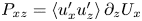 $P_{xz}=\langle u'_x u'_z\rangle \,\partial _z U_x$ starts declining due to a reduction in
  $\langle u'_x u'_z \rangle$ (not shown here for brevity). At
  $Nt \approx 4.5$, the contribution of the lateral production
  $P_{xy}$ exceeds that of the vertical production
  $P_{xz}$.
The reduction of  $\{P_{xz}\}$ in the
  ${Fr}=10$ wake coincides with the transition of
  $U_d$ to a slower decay rate. In figure 11(b), we note that
  $\{P_{xz}\}$ starts decaying faster than its unstratified counterpart for
  $3 < Nt < 4$ (or
  $30 < x < 40$). In figure 4(a), we see that this is the location where
  $U_d$ of the
  ${Fr} = 10$ spheroid wake starts deviating from the
  ${Fr} = \infty$ spheroid wake. At the same location that
  $\{P_{xz}\}$ starts decaying rapidly, there is a maximum in the buoyancy flux
  $\{B\}$ (figure 11e) and a slowdown in the growth of
  $L_V$ (figure 5a). Buoyancy is starting to affect the wake decay.
The initial value of  $\{P\}$ in the
  ${Fr}=2$ wake is higher than in the unstratified case. The distinct separation pattern and the vertical contraction of the mean flow (figure 5a) lead to an increase in the vertical shear and hence
  $\{P_{xz}\}$; see red dashed line in figure 11(b). This initially high value of
  $\{P_{xz}\}$ rapidly decays as
  $L_V$ increases, leading to a reduction in the vertical shear. Note that the beginning of the
  $U_d$-based NEQ regime at
  $Nt\approx {\rm \pi}$ also coincides with this reduction of
  $\{P_{xz}\}$. However, the mechanism at
  ${Fr}=2$ is different from that of the
  ${Fr}=10$ wake. Whereas at
  ${Fr}=10$, the reduction of
  $\langle u'_x u'_z \rangle$ causes the decay of
  $\{P_{xz}\}$, at
  ${Fr}=2$, the decay of
  $\langle u'_x u'_z \rangle$ is accompanied by a sudden reduction of
  $\partial _z U_x$ (not shown here). The reduction in vertical shear is driven by the expansion of
  $L_V$ due to lee wave modulation in figure 5(a).
As the modulation of the wake by the lee waves continues, the horizontal production is enhanced by the strong reduction in  $L_H$ (figure 5c) in the NEQ region for
  $7 < x < 20$. The value of
  $\{P_{xy}\}$ overtakes
  $\{P_{xz}\}$ at
  $Nt\approx 5$. The magnitude of
  $\{P_{xy}\}$ remains nearly constant until the end of the domain. Figure 11(f) shows the maximum of the horizontal mean shear (
 $\partial U_x/\partial y$), i.e.
  $\mathrm {max}_{(r,\theta =0)} \partial U_x/\partial y$, in the central streamwise-horizontal plane for both wakes. The mean shear in the
  ${Fr} = 2$ wake increases in the region
  $10 < x < 30$, exactly the region where the TKE decay starts plateauing (see figure 8a). The enhanced mean horizontal shear at
  ${Fr} =2$ prevents the horizontal production from decaying monotonically, unlike for
  ${Fr} = 10$.
Figure 11(c) shows the evolution of  $\{\varepsilon \}$ as a function of
  $x$ for
  ${Fr} = \infty$,
  $10$ and
  $2$ spheroid wakes. In the
  ${Fr} = 10$ case, the decay of
  $\varepsilon$ is similar to that of the unstratified wake until
  $Nt\approx 3$, after which the decay rate increases slightly. The
  ${Fr} = 2$ wake dissipation shows a sharper decay, until
  $x \approx 20$. After
  $x \approx 20$, the decay rate appears to be closer to the
  ${Fr} =\infty$ decay rate of
  $x^{-7/5}$ (ONS21).
Since the turbulent dissipation keeps decreasing monotonically in the  ${Fr} = 2$ spheroid wake (figure 11c), while the production tends to asymptote for
  $x>30$ (figure 11a), the value of
  $\{P\}/\{ \varepsilon \}$ becomes greater than
  $1$ in the
  ${Fr}=2$ spheroid wake (see figure 11d), explaining the rapid increase of TKE beyond
  $x \approx 30$. Note that the
  $\{P\}/\{ \varepsilon \}$ ratio oscillates with the characteristic wavelength of the lee waves, revealing the strong influence of wave-related buoyancy effects on the energetics of the
  ${Fr}=2$ wake.
One of the features of the arrival of the NEQ regime reported in previous studies is the radiation of internal gravity waves (Abdilghanie & Diamessis Reference Abdilghanie and Diamessis2013; De Stadler & Sarkar Reference De Stadler and Sarkar2012; Rowe et al. Reference Rowe, Diamessis and Zhou2020). In these spheroid wakes, we find that the integrated wave flux remains negligible compared with the other terms in the TKE budget and hence is not shown here. The small magnitude of the turbulent wave flux is consistent with the findings of Meunier et al. (Reference Meunier, Dizès, Redekopp and Spedding2018), who found that the magnitude of the wake-generated waves depends on the body drag coefficient – and the 6 : 1 spheroid has a very low drag compared with bluff bodies.
5.3. Early arrival of the Q2D regime in the ${Fr} = 2$ spheroid wake

Remember that the Q2D regime in stratified wakes is characterized by a faster decay of the mean defect velocity ( $U_d \sim x^{-3/4}$) and the organization of wake into distinct layers in the vertical direction. Due to the strong effects of buoyancy, the fluid motions are confined primarily to the horizontal plane. However, the vertical variations in the velocity profiles still exist during the Q2D regime, primarily in the form of layered structures.
A key difference between the  ${Fr} = 2$ disk and spheroid wakes is the early arrival of the Q2D regime in the spheroid wake. Whereas in the disk wake, CS20 did not observe a transition to the Q2D in a domain that extended up to
  $x = 125$ (
 $Nt = 62.5$), here we observe a transition at
  $x \approx 40$ (
 $Nt \approx 20$). The early transition in the spheroid wake is a consequence of the strong modulation of the intermediate wake by buoyancy, an effect that occurs for bodies with large aspect ratio (
 $L/D$) and, specifically, when
  ${Fr}$ is near its critical value
  ${Fr}_c = L/D{\rm \pi}$.
Figure 5(c) shows that  $L_H$ in the
  ${Fr} = 2$ spheroid wake contracts in the region
  $5 < x < 30$ as a response to the expansion of
  $L_V$ (figure 5a) by steady lee waves. This phenomenon leads to the ‘butterfly’ shaped structure of mean
  $U_x$ (figures 7d,e), which was also observed at a lower Reynolds number in Ortiz-Tarin et al. (Reference Ortiz-Tarin, Chongsiripinyo and Sarkar2019). In that study, which was performed at
  ${Re} = 10^4$, the spheroid wake at critical
  ${Fr}_c$ is relaminarized. Here, at a higher
  ${Re} = 10^{5}$, the flow response at the resonant state is quite different. The constriction of
  $L_H$ leads to an enhancement in the mean horizontal shear shown in figure 11(f). This enhancement slows down significantly the decay of horizontal production (figure 11b). While
  $\varepsilon$ continues to decay,
  $\{P\}/\{\varepsilon \}$ becomes
  $>1$, leading to an increase of TKE for
  $x >40$ (figure 8a). In figures 7(d–f), we also see the maximum TKE location moving to the wake axis from its off-centre location in the near wake. It is worth noting that the enhanced
  $\{P\}$ that acts as a source of TKE is a sink for the mean energy. The sharp increase in TKE leads to a faster decay of
  $U_d$, and the
  ${Fr} =2$ wake transitions to the Q2D regime early on, at
  $x \approx 40$.
In the disk wake,  $L_H$ is initially 3–4 times larger than in the spheroid wake. While the lee wave modulation of
  $L_H$ is present in the disk wake as well (figure 5d), its amplitude relative to the original value of
  $L_H$ is quite small. Hence the horizontal mean shear (not shown here) and the horizontal production in the
  ${Fr} = 2$ disk wake continue to decay, unlike in the spheroid wake.
The arrival of the Q2D regime in the spheroid wake is also accompanied by distinctive features of the Q2D regime reported in the literature previously. Figure 2(d) shows lateral meanders in the late  ${Fr} = 2$ wake, similar to the lateral meanders in temporal simulations in the literature (Brucker & Sarkar Reference Brucker and Sarkar2010; Diamessis et al. Reference Diamessis, Spedding and Domaradzki2011), albeit the temporal-simulation meanders occur much later in
  $Nt$ units. As noted during the discussion of spectra, the waviness in the late wake has characteristic frequency
  ${St} \approx 0.35$. The mean wake in the Q2D regime has a layered topology (figure 7f) as reported by Spedding (Reference Spedding2002) and Chongsiripinyo et al. (Reference Chongsiripinyo, Pal and Sarkar2017). The turbulence state in the Q2D regime is characterized by weak vertical fluctuations
  $u_z' \ll u'_h$ (Spedding Reference Spedding1997), with
  $\{E_{Kz}^{T}\}/\{E_{Kh}^{T}\} < 0.1$ at
  $x > 60$ – where subscript
  $h$ denotes the horizontal component of the fluctuations. Since the Q2D regime of the spheroid wake is in a relatively early phase, pancake vortices do not appear until the end of the simulation domain,
  $x = 80$.
5.4. Late transition to the NEQ regime in the ${Fr} = 10$ spheroid wake

At  ${Fr}=10$, the main difference between the disk and spheroid wakes is the location at which
  $U_d$ deviates from the unstratified counterpart, i.e. the transition point to the NEQ regime. In the spheroid wake, this transition occurs at
  $Nt\approx 3$, whereas in the disk it occurs at
  $Nt\approx 1$; compare the
  ${Fr} = 10$ curves between figures 4(a) and 4(b). The beginning of the NEQ regime is marked by a slowdown in the decay rate of
  $U_d$ in the stratified wake as compared with its unstratified counterpart. The NEQ regime is also characterized by the progressively increasing anisotropy between the horizontal and vertical components of TKE.
To understand better how this transition occurs, we look into the mean kinetic energy (MKE) transport equation. The TKE transport equation was given in (5.3). In a similar fashion, the MKE transport equation is given by
 \begin{equation} U_i\,\frac{\partial{E^M_K}}{\partial{x_i}}+\frac{\partial{T^M_i}}{\partial{x_i}}={-}P-\varepsilon^M+B^M, \end{equation}
where superscript  $M$ denotes the mean counterparts of terms in (5.3).
Figure 12(a) shows the area-integrated production  $\{P\}$ normalized by the Lagrangian change of the MKE (
 $\{E_K^{M}\}U_{\infty }/x$) in the disk and spheroid wakes at
  ${Fr} = \infty$ and
  $10$. Likewise, figure 12(b) shows the normalized area-integrated mean buoyancy flux
  $\{B^{M}\}$. Normalization by the Lagrangian change of MKE allows us to quantify the individual importance of each budget term to the change of MKE.

Figure 12. Area-integrated (a) production and (b) buoyancy flux in the disk and spheroid  ${Fr} = 10$ wakes. The unstratified wake (
 ${Fr} = \infty$) production is also shown in (a). The terms are normalized by the Lagrangian rate of change of their corresponding mean kinetic energy,
  $\{\delta _t E_K^{M}\} = \{E^{M}_K\}U_\infty /x$.
Broadly, the mean and turbulence quantities in stratified wakes deviate from their unstratified counterparts as a result of buoyancy. In the MKE transport equation, buoyancy can affect (a) the turbulence production  $P$ as an indirect effect, and (b) the MKE
  $\leftrightarrow$ MPE transfer, through the mean buoyancy flux
  $B^M$. In both the disk and spheroid
  ${Fr} = 10$ wakes, we find that the contribution of the mean buoyancy flux to the MKE transport is significantly smaller than the contribution of the production, particularly for
  $x \lessapprox 40$. Now turning to the area-integrated production in figure 12(a), we find that the production at
  ${Fr} = 10$ displays a strong reduction from the
  ${Fr} = \infty$ wake later in the spheroid at
  $x \approx 30$ (
 $Nt \approx 3$) compared with the disk, where a similar strong reduction occurs at
  $x \approx 10$ (
 $Nt \approx 1$). This explains the late transition of the spheroid wake to the NEQ regime, i.e.
  $U_d$ deviates from unstratified behaviour later (
 $Nt \approx 3$) for the spheroid than the
  $Nt \approx 1$ transition point for the disk.
The decreased production in the  ${Fr}=10$ wakes of both bodies is a consequence of the decreased
  $\langle u'_xu'_z\rangle$ correlation (not shown here for brevity) in stratified turbulent shear flows (Jacobitz, Sarkar & VanAtta Reference Jacobitz, Sarkar and VanAtta1997). In stratified wakes, this buoyancy effect has been observed experimentally by Spedding (Reference Spedding2002) and numerically by Brucker & Sarkar (Reference Brucker and Sarkar2010). The deviation between production of the
  ${Fr} = 10$ and
  $\infty$ wakes (figure 11a) is indeed caused by a reduction in the
  $\{P_{xz}\}$ component; see the blue dashed line in figure 11(b).
6. Evolution of the local flow state and its trajectory in the phase space
In previous sections, we showed how the spheroid and disk wakes do not transition between the 3-D, NEQ and Q2D regimes at the same  $Nt$. In this section, we examine the evolution of key local non-dimensional numbers describing the mean and fluctuating state to explore their roles. These non-dimensional numbers are local, streamwise-varying measures of stratification (Froude number) and the dynamical range of inertially dominated scales (Reynolds number). We also plot the trajectory of each wake in the Froude–Reynolds phase space.
The mean vertical Froude number ( ${Fr}_V$) and the turbulent vertical and horizontal Froude numbers (
 ${Fr}_v, {Fr}_h$) are defined as
 \begin{equation} {Fr}_V=\frac{U_d}{2 N L_V},\quad {Fr}_v=\frac{u'_h}{N l_v},\quad {Fr}_h=\frac{u'_h}{N L_{Hk}}, \end{equation}
where  $u_h'=(\langle u'^2_x\rangle +\langle u'^2_y\rangle )^{1/2}$ is the r.m.s. of the horizontal fluctuations, and
  $l^2_v=\langle u'^2_x+u'^2_y\rangle /\langle (\partial _zu'_x)^2+ (\partial _zu'_y)^2)\rangle$ is a vertical turbulent length scale (Riley & DeBruynKops Reference Riley and DeBruynKops2003).
The mean Froude number is defined consistently with the global Froude number ( ${Fr}=U_\infty /ND$), that is, with the wake full height
  $2L_V$. The turbulent Froude numbers are defined with turbulence length scales in the energy-containing range. Since the horizontal turbulent integral length scale (
 $l_h$) is not easy to compute in a spatially evolving flow, we use the TKE-based horizontal wake half-width (
 $L_{Hk}$) as a surrogate, following CS20. Here,
  $L_{Hk}$ at a downstream location
  $x$ is calculated by
  $E^{T}_K(y=L_{Hk},z=0, x) = 0.5E^T_{K}(y=0,z=0, x)$.
The mean vertical Froude number  ${Fr}_V$ (figure 13a) becomes
  $O(1)$ in both disk and spheroid wakes at the location at which the decay of
  $U_d$ slows down, signalling the beginning of the NEQ regime, marked by
  $Nt \approx 1$ for the disk and
  $Nt \approx 3$ for the spheroid. For the
  ${Fr} = 2$ cases,
  ${Fr}_V$ in the spheroid wake starts dropping faster beyond
  $x \approx 40$ – the streamwise location where the wake transitions from NEQ to the Q2D regime.

Figure 13. Evolution of the spheroid (solid lines) and disk (dashed lines) wakes at  ${Fr} = 2$ (red) and
  ${Fr} = 10$ (blue) in the non-dimensional parameter space: (a) local vertical mean Froude number
  ${Fr}_V$; (b) local vertical turbulent Froude number
  ${Fr}_v$; (c) local horizontal turbulent Froude number
  ${Fr}_h$; and (d) local horizontal Reynolds number.
The turbulent Froude numbers play a role analogous to those based on the mean. When their values become  $O(1)$, turbulence starts being affected by buoyancy. Here,
  ${Fr}_v$ is defined using
  $l_v$, which has a significance to shear instability. Defined with
  $l_v$,
  ${Fr}_v$ is proportional to
  $Ri^{-1/2}$, where
  $Ri$ is the Richardson number of the fluctuating shear (Riley & DeBruynKops Reference Riley and DeBruynKops2003; CS20). When
  ${Fr}_v$ becomes
  $O(1)$ (figure 13b) is also when the spanwise and vertical components of the TKE start showing anisotropy of the turbulence stress tensor, and
  $E^T_{Ky}>E^T_{Kz}$ as shown in figure 8 for the
  ${Fr}=2$ wakes. See also figure 8 of CS20.
The reader may notice that the four  ${Fr}_v=u'_h/Nl_v$ curves could collapse if plotted against
  $Nt$ instead of
  $x$. Indeed, these curves collapse in the
  ${Fr}_v\unicode{x2013}Nt$ plot for
  $1 < Nt < 10$, and the factor
  $5$ present between the curves in figure 13(b) is simply the ratio of buoyancy frequency
  $N$ between
  ${Fr}=2$ and
  ${Fr}=10$. This result points to the fact that the spheroid and disk wakes are at a sufficiently high
  ${Re}$ so that there is a range of small-scale wake turbulence with dynamics relatively unaffected by the large scales, and therefore by neither the shape of the wake generator nor buoyancy. Here,
  $u'_h/l_v$ is a quantity that reflects such dynamics, thus on dimensional grounds, it evolves as
  $u'_h/l_v \sim t^{-1}$ so that
  ${Fr}_v = u'_h/Nl_v \sim (Nt)^{-1}$. We note that buoyancy does affect large-scale wake features, which are affected by the body particularities – hence the lack of collapse in
  ${Fr}_V$. The values of the buoyancy Reynolds number
  ${Re}_b=\varepsilon/\nu N^2$ and the Reynolds number of the Taylor micro-scale
  ${Re}_\lambda =\sqrt {k} \lambda /\nu$, where
  $\lambda ^2=15\nu u'^{2}_x/\varepsilon$ (not included here for brevity), are very similar in magnitude for both disk and spheroid wakes at the two levels of stratification. This finding is consistent with the initial collapse of
  ${Fr}_v$ when plotted against
  $Nt$.
$Nt$.
In figure 13(c), the  ${Fr}=10$ wakes of both disk and spheroid reach
  ${Fr}_h \sim O(1)$ at
  $x\approx 10\unicode{x2013}20$, the location at which
  $\{E^T_K\}$ starts deviating from its unstratified counterpart (figures 8a,b). In the
  ${Fr}=2$ spheroid wake,
  ${Fr}_h<1$ throughout the domain, and
  $\{E^T_K\}$ deviates from the unstratified decay from the very beginning in both disk and spheroid wakes. Overall, we find that
  ${Fr}_h\sim O(1)$ is a good indicator of the deviation of
  $\{E^T_K\}$ from the unstratified counterpart. In contrast,
  ${Fr}_v \sim O(1)$ marks the location at which turbulence anisotropy between the vertical and spanwise components starts growing. Figure 13(d) shows the evolution of turbulence Reynolds number
  ${Re}_h = u'_hL_{Hk}/\nu$, with
  $u'_h$ being the intensity of horizontal turbulent fluctuations. The value of
  ${Re}_h$ (figure 13d) changes slowly as the wake evolves, remaining at
  $O(10^4$) for the disk wake, and at
  $O(10^3$) for the spheroid wake.
A consolidated view of the evolution of the state of fluctuations is provided in phase space (Brethouwer et al. Reference Brethouwer, Billant, Lindborg and Chomaz2007; de Bruyn Kops & Riley Reference de Bruyn Kops and Riley2019; Zhou & Diamessis Reference Zhou and Diamessis2019; CS20). In the phase-space portrait, one axis measures the buoyancy effect on the large scales through the turbulent Froude number ( ${Fr}_h$), and the other axis is a measure of Reynolds number that is not
  ${Re}_h$ but one that accounts for buoyancy in addition to inertia. Ozmidov-scale eddies are the largest eddies unrestrained by buoyancy. The Ozmidov scales
  $l_o=(\varepsilon /N^3)^{1/2}$ and
  $u_o=(\varepsilon /N)^{1/2}$ lead to the definition of
  ${Re}_b=u_ol_o/\nu = \varepsilon /\nu N^2$ as the so-called buoyancy Reynolds number. Another convenient measure of Reynolds number, which does not require explicit computation of the turbulent dissipation rate, is the buoyancy-weighted Reynolds number
  ${Re}_h\,{Fr}_h^2$ (Billant & Chomaz Reference Billant and Chomaz2001; Riley & DeBruynKops Reference Riley and DeBruynKops2003). The Reynolds numbers based on buoyancy tend to decrease with downstream distance as buoyancy increases progressively in importance and limits the range of scales that are susceptible to 3-D turbulent motions. As long as
  ${Re}_h\,{Fr}_h^2 > O(1)$, viscous effects do not dominate.
Following CS20, figure 14 shows the evolution all four wakes in the  ${Re}_h\,{Fr}_h^2\unicode{x2013}{Fr}_h$ phase space, where
  ${Re}_h = u'_hL_{Hk}/\nu$,
  $u'_h$ is the intensity of horizontal turbulent fluctuations. The flow evolves in the direction of the arrow from a state where buoyancy effects are weak (almost negligible) to a region characterized by the presence of stratified turbulence. Within the state of stratified turbulence, three different regimes can be demarcated: weakly, intermediately and strongly stratified turbulence (WST, IST and SST). Unlike the case of freely decaying turbulence, the mean velocity is also important here. Therefore, CS20 elected to distinguish between WST (where buoyancy begins to affect the mean velocity) and IST (where the turbulence anisotropy begins to be affected) as we do here. The SST regime is one where buoyancy effects on the large scales is very strong (
 ${Fr}_h \ll 1$), but nevertheless the value of
  ${Re}_h\,{Fr}_h^2$ is sufficiently large so that viscous effects are not dominant at the large scales.

Figure 14. Description of the trajectories of spheroid (solid lines) and disk (dashed lines) wakes in  ${Fr}_h\unicode{x2013}{Re}_h\,{Fr}_h^{2}$ phase space. Here,
  ${Fr} = 2$ and
  ${Fr} = 10$ are shown in red and blue, respectively. The dotted black line shows a
  ${Re}_h = \mathrm {const.}$ line in phase space.
The slope in the  ${Re}_h\,{Fr}_h^2\unicode{x2013}{Fr}_h$ plane is similar for both disk and spheroid wakes in the weak buoyancy and WST stages. The slope almost follows a line of constant
  ${Re}_h$, marked by a dashed line, signalling the slow evolution of
  ${Re}_h$ compared with that of
  ${Fr}_h$. However, there are significant differences in the way the spheroid wakes transverse the phase space. The spheroid wake starts out thinner than the disk wake, leading to larger local Froude numbers. Also, despite the body-based
  ${Re}$ being larger in the spheroid wake by a factor of 2, the turbulence intensity in the disk wake is higher, hence the
  ${Re}_h$ difference observed in figure 13(d). This difference in
  ${Re}_h$ can be seen in the horizontal offset between the disk and spheroid lines in the phase-space representation.
Despite the larger spheroid-body-based Reynolds number –  ${Re} = 10^5$ instead of
  ${Re} = 5\times 10^4$ – turbulence in the spheroid wake is unable to access either the the IST regime or the SST regime, while the disk wake is able to access these regimes of stratified turbulence. Furthermore, the increase in TKE, which is not observed in the
  ${Fr} = 2$ disk wake, reverses the trajectory of the
  ${Fr}=2$ spheroid wake. To the authors’ best knowledge, a reversing trend of phase-space trajectory has not been seen before in the stratified turbulence literature. These differences reveal that the phase-space evolution, at least for
  ${Fr} \leqslant 10$, depends on the features of the wake generator, e.g. its aspect ratio or the type of boundary layer separation.
Based on the phase-space portrait alone, one may hastily conclude that stratified slender-body wakes always experience a weaker buoyancy effect relative to bluff bodies. This is true for the  ${Fr} = 10$ case, at least for the limited
  $Nt$ simulation time, in terms of the relative amount of TPE (figure 10) and the vertical scale (
 $L_V$) deviation from the unstratified case – note that both are smaller in the spheroid wake than in the disk. However, we have also shown that for the
  ${Fr} = 2$ spheroid wake, compared with the disk wake, there is a much earlier onset of the Q2D regime. The mean and turbulence quantities are highly intertwined, and the strong modulation of the mean flow by steady lee waves of the high-aspect-ratio spheroid in the
  ${Fr} =2$ case ultimately leads to an early entry into the Q2D regime. Hence it is not entirely accurate to say that the slender-body wakes are weakly affected by stratification. The present work calls for a need to generalize the parameter space of
  $\{{Re},{Fr}\}$ in turbulent shear flows to account for the mean flow field (also possibly its instabilities) to build a more comprehensive understanding of buoyancy effects in shear flows. In the case of wakes, the shape of the body generator is brought into play through the mean flow as shown here.
7. Discussion and final remarks
The high-Reynolds-number stratified wake of a slender body has been studied using a high-resolution hybrid simulation. The wake generator is a 6 : 1 prolate spheroid with a tripped TBL, the diameter-based Reynolds number is  ${Re}=10^5$, and the Froude numbers, namely
  ${Fr}=U_\infty /ND=\{2,10,\infty \}$, take moderate to large values. By comparing the spheroid wake with the disk wake of Chongsiripinyo & Sarkar (Reference Chongsiripinyo and Sarkar2020), we are able to study the influence of the wake generator – slender versus bluff – in the establishment and evolution of stratified wakes.
The near wake of the 6 : 1 prolate spheroid with a TBL is characterized by a small recirculation region ( ${\sim }0.1 D$). The recirculation region is surrounded by small-scale turbulence that emerges from the boundary layer, and the flow does not show strong vortex shedding at the body (Jiménez et al. Reference Jiménez, Hultmark and Smits2010; Posa & Balaras Reference Posa and Balaras2016; Kumar & Mahesh Reference Kumar and Mahesh2018; Ortiz-Tarin et al. Reference Ortiz-Tarin, Nidhan and Sarkar2021). As a result, the wake is much thinner and develops more slowly than the wake of a bluff body like the disk, which has a large recirculation region (
 ${\sim }2 D$) and vortex shedding from the body (Nidhan et al. Reference Nidhan, Chongsiripinyo, Schmidt and Sarkar2020). These body-dependent features of the near wake were shown recently to affect the decay of the far wake in environments without density stratification (Ortiz-Tarin et al. Reference Ortiz-Tarin, Nidhan and Sarkar2021). In the present stratified simulations, we also find substantial differences in the decay of the disk and spheroid wake. In particular, we find that the starting locations of the non-equilibrium (NEQ) and the following Q2D regions of wake deficit velocity depend on the wake generator.
At  ${Fr}=2 \approx (L/D)/{\rm \pi}$, the wake of a 6 : 1 prolate spheroid is in a resonant state. The half-wavelength of the lee waves is equal to the body length, and as a result, the flow separation and the wake are strongly modulated by the waves. Whereas previous works had described this regime in laminar-separation configurations of a sphere (Hanazaki Reference Hanazaki1988; Chomaz et al. Reference Chomaz, Bonneton, Butet, Perrier and Hopfinger1992) and a 4 : 1 spheroid (Ortiz-Tarin et al. Reference Ortiz-Tarin, Chongsiripinyo and Sarkar2019), the present results show that the influence of the waves persists even at high Reynolds numbers and with the separation of a TBL. At
  ${Fr}=2$, the flow and the turbulence in the spheroid wake evolve very differently from the disk wake. Both the lack of strong shedding in the near wake (Ortiz-Tarin et al. Reference Ortiz-Tarin, Nidhan and Sarkar2021), and the strong modulation of the mean flow by the lee waves, lead to a wake with vertical and horizontal profiles of mean velocity that depart strongly from Gaussian. These features are not observed in the disk wake at
  ${Fr} =2$, which shows a vertically squeezed Gaussian topology and a weak imprint of lee waves on the wake dimensions.
At  ${Fr} =2$, both disk and spheroid wakes transition to the NEQ regime at
  $Nt\approx {\rm \pi}$. However, the transition to the Q2D regime – with enhanced wake decay relative to the NEQ regime – is very different; whereas the spheroid wake transitions at
  $Nt\approx 15$, the disk wake does not access the Q2D regime in a domain that spans
  $Nt\approx 60$. Other bluff bodies, e.g. the towed sphere (Spedding Reference Spedding1997), show transition to the Q2D regime at
  $Nt \approx 50$, a location that is also delayed with respect to the spheroid wake. The early transition to the Q2D regime of the spheroid wake is driven by its strong modulation – horizontal contraction and expansion of the wake width – in response to the vertical contraction and expansion by the lee waves. This modulation has a particularly strong effect on the slender wake of a spheroid where the horizontal contraction is a large fraction of the wake width. The early start of the Q2D regime in the spheroid wake is accompanied by a sustained increase of turbulent kinetic energy (TKE), driven by an increase of the horizontal mean shear that acts on the turbulence of the separated boundary layer. The TKE increase is limited to the horizontal velocity, with the spanwise component being strongest, having almost an order of magnitude larger energy than the vertical. Although coherent vortical structures and spanwise flapping are seen in the horizontal motion, pancake eddies are incipient and not fully formed at the end of the domain,
  $x/D = 80$.
At  ${Fr}=10$ also, there are differences between the disk and spheroid wakes. Particularly in the spheroid wake, the beginning of the NEQ stage occurs later, at
  $Nt\approx 3$ instead of
  $Nt\approx 1$ (
 $x\approx 30$ instead of
  $x \approx 10$). The difference in the start of the NEQ can be attributed to the value of the local mean Froude number
  ${Fr}_V=U_d/2NL_v$. As noted previously, the spheroid wake is thinner than the disk wake, and the mixing in the near wake is weaker; as a result, the defect velocity in the intermediate wake is larger. These features increase the value of the spheroid wake local Froude number and delay the onset of the buoyancy effect that gives rise to the NEQ regime. In addition, the analysis of the mean kinetic energy (MKE) transport terms shows that the onset of the buoyancy effect on the mean flow of both disk and spheroid
  ${Fr}=10$ wakes is associated with the decreased energy transfer from MKE to TKE.
Taking the unstratified case as a baseline, the effect of buoyancy in the spheroid  ${Fr}=10$ wake is observed earlier (at
  $Nt \approx 1$) on the decay of the TKE than its effect (at
  $Nt \approx 3$) on the decay of
  $U_d$. In the spheroid wake at
  ${Fr} = 10$, the transfer from TKE to TPE is responsible for the enhanced decay of TKE at
  $Nt \approx 1$. On the other hand, the decrease in turbulent production at a farther downstream distance (compared with the disk
  ${Fr} = 10$ wake) in the spheroid
  ${Fr}=10$ wake is responsible for the slowed decay of the mean defect velocity at
  $Nt \approx 3$. The decrease in the production is caused by a reduction in the
  $\langle u'_xu'_z\rangle$ correlation (Jacobitz et al. Reference Jacobitz, Sarkar and VanAtta1997; Spedding Reference Spedding2002; Brucker & Sarkar Reference Brucker and Sarkar2010).
Meunier & Spedding (Reference Meunier and Spedding2004) compared the evolution far into the stratified wake, up to  $x \approx 8000$, among several body shapes that also included a 6 : 1 prolate spheroid and a circular disk. The body Reynolds number was
  ${Re} = 5000$, and their diameter-based Froude numbers were
  ${Fr} = 4$ and
  $16$. When normalized using
  $D_{eff} = D \sqrt {C_{D}/2}$ instead of
  $D$, the evolution of the peak defect velocity of different wake generators exhibited approximate collapse for
  $Nt \gtrapprox 50$ (see their figure 5b) with a Q2D decay rate
  ${\sim }x^{-0.75}$. Similarly, the wake width in the horizontal of different shapes approximately collapsed for
  $x/D_{eff} > 400$ to exhibit a growth rate of
  ${\sim }x^{0.35}$. Since their 6 : 1 spheroid data start from
  $x/D \approx 100$ (see their figure 5a), a direct comparison is not possible with our simulations that end at
  $x/D = 80$.
With regard to the mean defect decay, a major difference between Meunier & Spedding (Reference Meunier and Spedding2004) and our results is that the transition to Q2D power-law behaviour appears earlier, at  $Nt \approx 15$, in the
  ${Fr} = 2$ spheroid wake. The value of
  ${Re} = 10^5$ in the spheroid wake is larger here, and it is possible that the features that we have linked to the early onset of the Q2D stage for the spheroid
  ${Fr} = O(1)$ wake – i.e. the instability that leads to horizontal meanders and also the enhanced TKE production – are inhibited by viscous damping at the lower
  ${Re}$ of the experiments.
The present simulations, of both the disk and the spheroid, do not extend into the very-far-wake regime reached by the experiments of Meunier & Spedding (Reference Meunier and Spedding2004). Future hybrid simulations or experimental work at higher  ${Re}$ that probe the very far wake would clearly be useful. At any given
  ${Re}$ and
  ${Fr}$, it will also be of interest to look at how tripping affects the wake evolution for the different body shapes.
The simulations show that the buoyancy time scale  $Nt$ alone is not sufficient to determine the state of the wake decay for both generators. However, we find that the values of the local turbulent and mean Froude numbers can be a good proxy to describe some aspects of the wake state. For both disk and spheroid wakes,
  ${Fr}_V=U_d/2NL_v$ becomes
  $O(1)$ at the location at which the decay of
  $U_d$ slows down;
  ${Fr}_h=u'_h/N L_{Hk} \sim O(1)$ marks the location at which the area-integrated TKE of the stratified wake starts deviating from the unstratified case; and
  ${Fr}_v=u'_h/N l_v \sim O(1)$ signals the location at which anisotropy between the different TKE components starts growing.
The buoyancy-weighted Reynolds number ( ${Re}_h\,{Fr}_h^{2}$) has been used widely in stratified flow as a convenient surrogate for the buoyancy Reynolds number (
 ${Re}_b = \varepsilon /\nu N^2$) since it displays similar trends during the flow evolution and the two quantities can be shown to be proportional using classical inviscid scaling of the turbulent dissipation rate. The surrogacy is true for the stratified wakes considered here, except for the spheroid
  ${Fr} = 2$ wake after its entry into the stage of Q2D wake decay. The horizontal fluctuation energy
  ${Fr}_h$ therefore increases owing to horizontal meanders and flapping of the flow. However,
  $\varepsilon$ continues to decrease, albeit at a reduced rate relative to the NEQ regime. The value of
  ${Re}_b = O (10)$ is not high in the Q2D regime realized here at
  ${Fr} =2$. It remains to be seen if, in the Q2D regime at even higher body-based Reynolds numbers, the equivalence between
  ${Re}_h\,{Fr}^2_h$ and
  ${Re}_b$ is recovered, and whether the unusual upward trajectory seen here in
  ${Fr}_h\unicode{x2013}{Re}_h\,{Fr}_h^2$ phase space is also seen in
  ${Fr}_h\unicode{x2013}{Re}_b$ space. The duration of the upward trajectory in phase space until the eventual downward shift toward the viscous regime is also of interest.
The differences between bluff-body (disk) and slender-body (6 : 1 spheroid) wakes illustrate the difficulty of finding a universal scaling for the high- ${Re}$ stratified wake. The initial magnitude of
  $U_d$ for different wake generators and levels of stratification can be scaled roughly with the global
  ${Fr}$ and the body drag coefficient (Meunier & Spedding Reference Meunier and Spedding2004). However, the start and the duration of the NEQ regime cannot be assumed to be independent of the wake generator. We find that rather than a particular
  $Nt$, the local mean Froude number is a good proxy for the onset of the NEQ regime in the mean defect velocity, and the values of local turbulent Froude number provide guidance for the behaviour of TKE, e.g. the onset of the buoyancy effect as well as the location at which the ratio of vertical to horizontal TKE starts decreasing. We are unable to connect the Froude number to the Q2D regime transition of the wake. More numerical and experimental work spanning different wake generators, different sources of turbulence (including freestream turbulence) and longer downstream distances will be instrumental in building a comprehensive picture of the effect of initial/boundary conditions on subsequent wake evolution.
Acknowledgements
Dr K. Chongsiripinyo is thanked for useful discussions and for disk simulations. We thank the anonymous reviewers for their helpful comments.
Funding
We gratefully acknowledge the support of Office of Naval Research grant N00014-20-1-2253.
Declaration of interests
The authors report no conflict of interest.
Author contributions
J.L.O.-T. and S.N. contributed equally to this paper and are co-first authors.


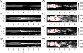


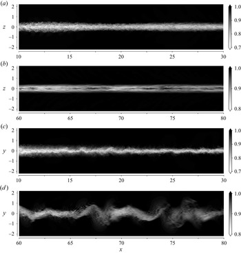

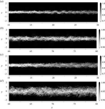


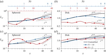

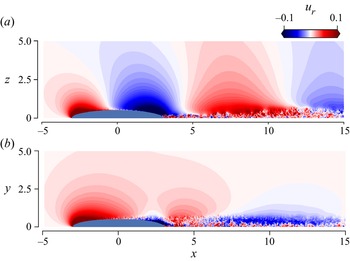

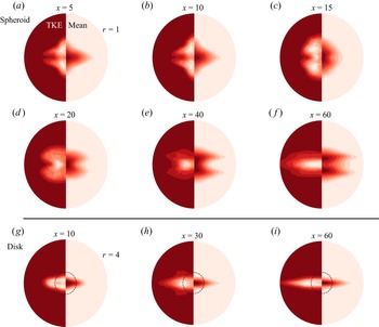


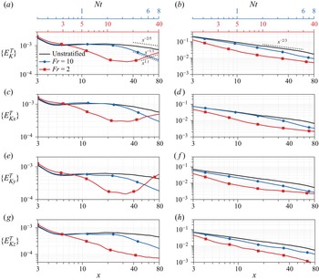


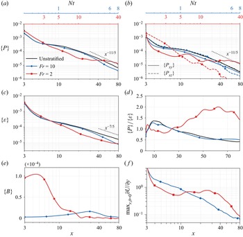


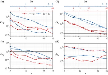


 Open access