


1. Introduction
Turbulent shear flows over porous walls are frequently encountered in the natural environment and industrial applications, such as oil wells, catalytic reactors, heat exchangers and porous river beds, to name but a few (Bottaro Reference Bottaro2019). As the blocking effect of the wall is relaxed, the porous bed allows for mass, momentum and energy exchange across the permeable interface, and a transitional layer forms as a buffer between the turbulent surface and laminar subsurface flows (Breugem, Boersma & Uittenbogaard Reference Breugem, Boersma and Uittenbogaard2006; Manes, Poggi & Ridolfi Reference Manes, Poggi and Ridolfi2011; Fang et al. Reference Fang, Xu, He and Dey2018; Kim et al. Reference Kim, Blois, Best and Christensen2020; Suga, Okazaki & Kuwata Reference Suga, Okazaki and Kuwata2020). Previous studies of turbulent flow over permeable beds have addressed the dependence of flow physics on the wall permeability (Finnigan Reference Finnigan2000; Voermans, Ghisalberti & Ivey Reference Voermans, Ghisalberti and Ivey2017). The turbulent surface flow is similar to that of a canonical boundary layer when the interfacial permeability is low, where the near-wall structures are less disrupted (Breugem et al. Reference Breugem, Boersma and Uittenbogaard2006). As the permeability increases, large-scale vortical structures emerge in the surface flow, which are attributed to Kelvin–Helmholtz (KH) type instabilities from inflection points of the mean velocity profile (Finnigan Reference Finnigan2000; Jiménez et al. Reference Jiménez, Uhlmann, Pinelli and Kawahara2001; Breugem et al. Reference Breugem, Boersma and Uittenbogaard2006; Manes et al. Reference Manes, Poggi and Ridolfi2011; Nepf Reference Nepf2012). Additionally, characteristics of the near-wall cycle, e.g. streaks and streamwise vortices, are substantially weakened in the presence of porous walls compared to smooth-wall turbulence. This is summarized by the theory of Manes et al. (Reference Manes, Pokrajac, McEwan and Nikora2009, Reference Manes, Poggi and Ridolfi2011) via two competing mechanisms in the flow: the formation of wall-attached eddies and the disruption by shear layer instabilities. The balance between the two mechanisms is controlled by the wall permeability.
More recently, the application of porous media in drag reduction has inspired a series of in-depth studies on wall permeability. Rosti, Cortelezzi & Quadrio (Reference Rosti, Cortelezzi and Quadrio2015) conducted a parameter study with coupled direct numerical simulation (DNS) and volume-averaged Navier–Stokes (VANS) simulation. They focused on porous media with relatively low permeability where the inertial effects within the porous layer can be neglected. It was shown that the roles of permeability and porosity are decoupled, and the effects of permeability are dominant with respect to the effects of porosity. In a following study, Rosti, Brandt & Pinelli (Reference Rosti, Brandt and Pinelli2018) found that the total drag could be reduced by more than  $20\,\%$ through adjusting directional properties of the permeability. When streamwise and spanwise diagonal components of the permeability tensor (streamwise and spanwise permeability) are larger than the wall-normal component (wall-normal permeability), the low- and high-speed streaks are more elongated in the streamwise direction, which leads to an enhanced slip velocity and net drag decrease. Wall-normal fluctuations are also suppressed, leading to a decrease in total shear stress.
Gómez-de Segura & García-Mayoral (Reference Gómez-de Segura and García-Mayoral2019) further explored the ability of anisotropic permeable substrates to reduce turbulent skin friction. It was observed that the drag reduction is proportional to the difference between the streamwise and spanwise permeabilities for low-permeability substrates. This is consistent with the conclusion of previous studies that streamwise-preferential complex surfaces can reduce drag in turbulent flows. Garcia-Mayoral & Jiménez (Reference Garcia-Mayoral and Jiménez2011) and Abderrahaman-Elena & García-Mayoral (Reference Abderrahaman-Elena and García-Mayoral2017) noted the degradation of drag reduction performance when wall-normal permeability increases, which is associated with the appearance of KH-type eddies. Kuwata & Suga (Reference Kuwata and Suga2017) investigated the influence of the anisotropic permeability tensor of the porous medium in a higher-permeability regime. In contrast with the result for low-permeability porous media (Rosti et al. Reference Rosti, Brandt and Pinelli2018; Gómez-de Segura & García-Mayoral Reference Gómez-de Segura and García-Mayoral2019), it was found that streamwise and spanwise permeabilities enhance turbulence whilst vertical permeability itself does not. In particular, the enhancement of turbulence is remarkable over porous walls with streamwise permeability, as it allows the development of streamwise large-scale perturbations induced by KH instability. This is also confirmed by Suga et al. (Reference Suga, Okazaki and Kuwata2020), who observed that turbulence over and under the porous surfaces is roughly insensitive to the wall-normal permeability compared with the streamwise permeability.
In addition to the statistical properties of turbulence over permeable walls, the dynamics of the coupling between the surface flow and subsurface flow have also attracted numerous studies. Breugem et al. (Reference Breugem, Boersma and Uittenbogaard2006) reported the correlation between the sign of the wall-normal flow transporting fluid across the permeable interface and the sign of the fluctuating streamwise velocity in the surface flow. This linkage was confirmed by the experiments of Kim et al. (Reference Kim, Blois, Best and Christensen2018) and the DNS of Chu et al. (Reference Chu, Wang, Yang, Terzis, Helmig and Weigand2021). Manes et al. (Reference Manes, Pokrajac, McEwan and Nikora2009) uncovered two types of turbulence within the porous bed using spectral analysis. The first type is periodic large-scale motions with a wavelength 10 times the eddy turnover time. They speculated that these large-scale motions are generated remotely in the flow surface and imposed onto the flow below the permeable interface. The second type is small-scale turbulent events in the transitional layer, which may be associated with pore-scale vortices generated locally within the porous medium.
Kuwata & Suga (Reference Kuwata and Suga2016) used proper orthogonal decomposition (POD) to extract the large-scale pressure perturbations across a permeable interface, which are associated with KH-type eddies. Motlagh & Taghizadeh (Reference Motlagh and Taghizadeh2016) examined the POD spatial mode to inspect the influence of wall permeability on the dynamical features of flow across the permeable interface. They revealed that the permeability of the wall modifies the size and even the shape of the large-scale, energetic dominant structures that stem from the KH instability. A recent study by Kim et al. (Reference Kim, Blois, Best and Christensen2020) examined the amplitude modulation in permeable-wall turbulence. The spatiotemporal signatures of amplitude modulation were also characterized using correlation map and conditional averaging techniques. The connections between large-scale regions of high/low streamwise momentum in the surface flow, downwelling/upwelling across the permeable interface, and enhancement/suppression of small-scale turbulence were also observed. Moreover, it was found that porous media with rough surfaces are subject to stronger penetration of the flow into the permeable bed modulated by large-scale structures in the surface flow.
Despite the latest advances in the field, the dynamics of the mass and momentum transfer across the interface of porous media are far from being settled. Although we do have a solid knowledge of the connection between flow structures resulting from the surface–subsurface interaction, the fundamental cause-and-effect relations of these fluid motions are rarely inspected. To what extent does the outer turbulence determine the flow inside porous media and vice versa? These questions cannot be addressed by correlation, spectral analysis and traditional mode decomposition methods (e.g. POD), as these approaches do not provide the directionality and time asymmetry required to quantify causation (Kantz & Schreiber Reference Kantz and Schreiber2004; Pearl Reference Pearl2009). In recent years, new linear dynamics tools have emerged to study the structure and dynamics of turbulent flow. Examples are dynamic mode decomposition (DMD) (Schmid Reference Schmid2010), spectral proper orthogonal decomposition (SPOD) (Towne, Schmidt & Colonius Reference Towne, Schmidt and Colonius2018), etc. DMD and SPOD allow the original nonlinear dynamics of the flow to be approximated by a linear system, which is suitable for the low-order modelling of quasi-linear systems. Nonetheless, for highly nonlinear dynamics such as the coupling of free flow and porous media, it is unclear whether the linear modes extracted by these tools alone are enough to explain cause-and-effect relationships in the original nonlinear system.
Recently, Lozano-Durán, Bae & Encinar (Reference Lozano-Durán, Bae and Encinar2020) highlighted the importance of causal inference in fluid mechanics (see also Lozano-Durán et al. Reference Lozano-Durán, Constantinou, Nikolaidis and Karp2021) and proposed to leverage information-theoretic metrics to explore causality in turbulent flows. In particular, Lozano-Durán et al. (Reference Lozano-Durán, Bae and Encinar2020) examined the causal interactions of energy eddies in wall-bounded turbulence using transfer entropy. The concept of transfer entropy was first proposed by Schreiber (Reference Schreiber2000) as a tool to evaluate the directional information transfer between a source signal and receiver signal. Information transfer between two time series is typically defined as the dependence of the future state of the receiver on the previous state of the source. Schreiber's (Reference Schreiber2000) definition of transfer entropy is essentially predictive information transfer and measures the average information contained in the source about the next state of the destination that was not already contained in the destination's past. In this respect, transfer entropy quantifies the statistical coherence between temporally evolving systems in a directional and dynamic manner. In this study, we conduct a DNS of a fully resolved interface and porous domain, and follow the analysis of Lozano-Durán et al. (Reference Lozano-Durán, Bae and Encinar2020) to quantify the causality between the interaction of surface and subsurface flow. Traditional tools such as spectral and correlation analysis are also provided to complement the analysis.
The work is organized as follows. We present the details of the DNS dataset in § 2. In § 3, coupling between inner and outer flow structures will be inspected in detail using a series of tools, e.g. spectral analysis, linear coherent spectra, as well as transfer entropy. The object is to illustrate the asymmetry in the interaction of surface–subsurface flow. Finally, conclusions are offered in § 4.
2. Numerical simulations
The three-dimensional incompressible Navier–Stokes equations are solved in non- dimensional form,
 \begin{equation} \frac{\partial u_j}{\partial x_j}=0, \quad \frac{\partial u_i}{\partial t}+\frac{\partial u_i u_j}{\partial x_j}={-}\frac{\partial p}{\partial x_i}+\frac{1}{Re}\frac{\partial^2 u_i} {\partial x_j \partial x_j}+\varPi \delta_{i1}, \end{equation}
where  $\varPi$ is a constant pressure gradient in the mean-flow direction. The governing equations are non-dimensionalized by normalizing lengths by the half-width of the whole simulation domain $H$ (figure 1a), velocities by the averaged bulk velocity $U_b$ of the free-flow region ( $y/H=[0,1]$), such that time is non-dimensionalized by $H/U_b$. The spectral/ $hp$ element solver Nektar++ (Cantwell et al. Reference Cantwell, Sherwin, Kirby and Kelly2011; Chu et al. Reference Chu, Wu, Rist and Weigand2020; Pandey et al. Reference Pandey, Chu, Weigand, Laurien and Schumacher2020) is used to discretize the numerical domain containing complex geometrical structures. The solver allows for arbitrary-order spectral/ $hp$ discretizations with hybrid-shaped elements. The time stepping is performed with a second-order mixed implicit–explicit (IMEX) scheme. The time step is fixed to $\Delta T/(H/U_b)=5\times 10^{-4}$.

Figure 1. (a) Configuration of the computational domain; (b) corresponding cylinder radius of each porosity case; and (c) variation of normalized diagonal components of the permeability tensor  $\sqrt {K}_{\alpha \alpha }^{{p+}}$ and Forchheimer coefficients $C_{\alpha \alpha }^{{p+}}$ with porosity.
Hereafter, the velocity components in the streamwise  $x$, wall-normal $y$ and spanwise $z$ directions are denoted as $u$,
$u$,  $v$ and $w$, respectively. The domain size ( $L_x/H \times L_y/H \times L_z/H$) is $10 \times 2 \times 0.8{\rm \pi}$. The lower half ( $y/H=[-1,0]$) contains the porous medium and the upper half ( $y/H=[0,1]$) is the free channel flow. The porous layer consists of 50 cylindrical elements along the streamwise direction and five rows in the wall-normal direction, as illustrated in figure 1(a). The distance between two neighbouring cylinders is fixed at $D/H=0.2$.
The no-slip boundary condition is applied to the cylinders, the upper wall and the lower wall. Periodic boundary conditions are used in the streamwise and spanwise directions. The geometry is discretized using quadrilateral elements on the  $x - y$ plane with local refinement near the interface. High-order Lagrange polynomials (polynomial order $P=5 - 9$) are used within each element in the $x - y$ plane. The spanwise direction is extended with a Fourier-based spectral method.
Six DNS cases are performed with varying porosity  $\varphi =0.4$– $0.9$, which is defined as the ratio of the void volume to the total volume of the porous structure. The parameters of the simulated cases are listed in table 1, where the cases are named after their respective porosity. The superscripts $(\cdot )^{{p}}$ and $(\cdot )^{{s}}$ represent variables of permeable wall and top smooth wall sides, respectively. Variables with superscript $+$ are scaled by friction velocities $u_\tau$ of their respective side and viscosity $\nu$. Note that the distance between cylinders is fixed, and the porosity is changed by varying the radius of the cylinders. The relation between porosity $\varphi$ and cylinder radius $r$ is shown in figure 1(b). The normalized cylinder radius is in the range $r^{{p}+}=42$– $52$ for all the cases tested (see table 2) such that the effect of surface roughness is assumed to be on a similar level. The Reynolds number of the top wall boundary layer is set to be $Re_\tau ^{s}=\delta ^{s}u_\tau ^{s}/\nu \approx 180$ for all cases ( $\delta$ is the distance between the position of maximum streamwise velocity and the wall). In this manner, changes in the top wall boundary layer are minimized. On the top smooth wall side, the streamwise cell size ranges from $4.1\le \Delta x^{{s}+}\le 6.3$ and the spanwise cell size is below $\Delta z^{{s}+}=5.4$. On the porous-medium side, $\Delta z^{{p}+}$ is below 8.4, whereas $\Delta x^{{p}+}$ and $\Delta y^{{p}+}$ are enhanced by polynomial refinement of the local mesh (Cantwell et al. Reference Cantwell, Sherwin, Kirby and Kelly2011). The total number of grid points ranges from 88 $\times 10^6$ (case C04) to 582 $\times 10^6$ (case C09). Each cylinder in the porous domain is resolved with 80–120 grids along the perimeter.
Table 1. Simulation parameters. The porosity of the porous-medium region is  $\varphi$; the friction Reynolds numbers for the porous and impermeable top walls are $Re_{\tau }^{{p}}$ and $Re_{\tau }^{{s}}$, respectively; and $\Delta x^{{p}+}$/ $\Delta y^{{p}+}$/ $\Delta z^{{p}+}$ and $\Delta x^{{s}+}$/ $\Delta y^{{s}+}$/ $\Delta z^{{s}+}$ are the respective grid spacings in wall units of porous wall and top wall, respectively.

Table 2. Characteristics of the porous media:  $\sqrt {K_{\alpha \alpha }}^{{p}+}$ and $C_{\alpha \alpha }^{{p+}}$ are the diagonal components of the permeability tensor and Forchheimer coefficient, respectively, in the direction of $\alpha$ ( $\alpha \in \{x, y,z \}$); and $r^{{p+}}$ is the radius of the cylinders. All the variables are normalized using $u_\tau ^{{p}}$ and $\nu$.

The diagonal components of the permeability tensor  $K_{\alpha \alpha }$ and the Forchheimer tensor $F_{\alpha \alpha }$ are measured by DNS of only the porous-medium region. For the measurement of permeability along the $\alpha$ axis of the porous medium, the domain boundaries parallel to the $\alpha$ axis are periodic. The diagonal components of the permeability Forchheimer tensors are calculated using the Darcy–Forchheimer equation,
 \begin{equation} \langle u_i\rangle={-}\frac{K_{ij}}{\mu}\frac{\partial \langle p \rangle^f}{\partial x_j}-F_{ij}\langle u_j\rangle , \end{equation}
where  $\langle u_i\rangle$, $\langle p \rangle ^f$ and $\mu$ are the superficially volume-averaged velocity, the volume-averaged fluid-phase pressure and the dynamic viscosity of the fluid, respectively. The superscript ‘ $f$’ denotes a value in the fluid phase. The Forchheimer tensor $F_{ij}$ is modelled as $F_{ij}=C_{ij}|\langle \boldsymbol {u}\rangle |/\nu$, where $|\cdot |$ denotes the modulus. Note that, for a porous medium whose configuration is symmetric in the $x$,
$x$,  $y$ and $z$ directions, the permeability and Forchheimer tensors become diagonal (Suga et al. Reference Suga, Okazaki and Kuwata2020).
The measured permeabilities  $K_{\alpha \alpha }$ and Forchheimer coefficients $C_{\alpha \alpha }$ are listed in table 2, and their relation with porosity is shown in figure 1(c). The normalized permeability $\sqrt {K_{\alpha \alpha }}^{{p}+}=\sqrt {K_{\alpha \alpha }}u_\tau ^{{p}}/\nu$ grows almost exponentially with porosity. According to Voermans et al. (Reference Voermans, Ghisalberti and Ivey2017), cases C04 and C05, whose $\sqrt {K_{xx}}^{{p}+}$, $\sqrt {K_{yy}}^{{p}+}$ and $\sqrt {K_{zz}}^{{p}+}$ are well below 10, belong to the transitional regime where both attached eddies and KH eddies exist. Cases C06–C09 belong to the highly permeable regime where KH eddies prevail since $\sqrt {K_{\alpha \alpha }}^{{p}+}$ is close to or above 10. The Forchheimer tensors account for the nonlinear part of the relation between pressure drop and flow rate. The spanwise component $C_{zz}$ is zero for all the cases, while the streamwise and wall-normal components ( $C_{xx}$ and $C_{yy}$) are non-zero. The normalized Forchheimer coefficients $C_{xx}^{{p+}}$ and $C_{yy}^{{p+}}$ are relatively small for porosity $\varphi =0.4$–0.6, where Darcy's law works well. The nonlinear term becomes non-negligible for higher-porosity cases.
3. Results
The current section will start with the basic statistics (§ 3.1) and instantaneous flow fields (§ 3.2) to offer a general impression of the flow in the vicinity of the permeable interface. Then, § 3.3 will show the spectral density and linear coherence spectra (LCSs), providing insights into the surface–subsurface interactions from a scale-specific perspective. The tool of transfer entropy will be introduced in § 3.4 to unravel the asymmetry and directionality in the coupling process.
3.1. Mean velocity and turbulent kinetic energy profiles
The mean statistics of all the cases are briefly discussed here to outline the impact of porosity on surface and subsurface flow. Figure 2(a,b) shows the mean profiles for the streamwise velocity  $\langle \bar u \rangle$ and turbulent kinetic energy (TKE) $\langle \bar q\rangle =\langle \overline {u'u'+ v'v'+w'w'}\rangle /2$ normalized by $u_\tau ^{{s}}$. The operators $\langle \cdot \rangle$ and $\overline {(\cdot )}$ represent the spatial average in the $x$–
$x$– $z$ plane and the temporal average, respectively, and the prime denotes turbulent fluctuations, $\phi '=\phi -\bar {\phi }$. The profiles of an impermeable smooth-wall channel from Hoyas & Jiménez (Reference Hoyas and Jiménez2008) are also included for comparison. For increasing wall porosity, the mean velocity profile becomes more skewed towards the top wall as a consequence of the higher skin friction on the porous wall (Breugem et al. Reference Breugem, Boersma and Uittenbogaard2006). Below the interface ( $y=0$), the mean velocity profiles exhibit a clear inflection point, which is typically associated with KH-type instabilities responsible for additional turbulent structures (Manes et al. Reference Manes, Poggi and Ridolfi2011). This is partly substantiated by figure 2(b), which shows that the TKE below and above the interface is significantly enhanced for higher porosity considered here ( $\varphi =0.7$–0.9). In the following sections, we illustrate how the change of flow structures in the interface region affects the interaction between surface and subsurface flow.

Figure 2. (a) Mean streamwise velocity  $\langle \bar u\rangle$ normalized by $u_\tau ^{{s}}$; and (b) mean TKE profiles $\langle \bar {q}\rangle$ normalized by $(u_\tau ^{{s}})^2$. Profiles of impermeable smooth-wall channel from Hoyas & Jiménez (Reference Hoyas and Jiménez2008) for $Re_\tau =180$ are superimposed in thin dashed lines for comparison.
3.2. Upwelling and downwelling events
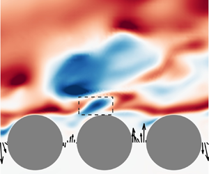
The upwelling/downwelling events transport fluid directly across the interface, which provide an intuitive picture of the interaction process. Examples of typical upwelling and downwelling events are captured in figure 3 for case C05 ( $\varphi =0.5$). During the upwelling event (figure 3a, $x/D=1$), a small amount of fluid is ejected from beneath the interface ( $tU_b/D=0$), which later becomes a low-speed bulb above the interface ( $tU_b/D=0.3$– $0.6$) to finally merge with a large low-speed structure downstream ( $tU_b/D=0.9$). During the downwelling event (figure 3b, $x/D=1$), a portion of low-speed fluid is absorbed into the porous medium ( $tU_b/D=0$). The low-speed structure is later separated into two structures as the upper part is convected downstream ( $tU_b/D=0.3$– $0.9$). The observations from the instantaneous fields also suggest that upwelling/downwelling events are subjected to the modulation of large-scale motions in the free-flow region. Specifically, the upwelling events at the gaps are often related to large-scale low-speed structures above the interface (see figure 3a, at $y/D=0.5$), while downwelling events are usually associated with high-speed structures (see figure 3b, at $y/D=0.5$). This connection was also observed by Kim et al. (Reference Kim, Blois, Best and Christensen2018), and it is further discussed in the following sections. In addition, the momentum flux between neighbouring gaps is usually negatively correlated, i.e. upwelling and downwelling events usually occur side by side, probably due to the constraint imposed by continuity at the interface.

Figure 3. Instantaneous  $u'$ fields (C05) during (a) an upwelling event and (b) a downwelling event. Fluctuation velocity $(u',v')$ in the porous-medium region is illustrated by vectors, which are normalized to unit length.
3.3. Spectral density and linear coherence spectra
It is known that the flow structure near a permeable interface is characterized by a broad spectrum of length scales (Manes et al. Reference Manes, Poggi and Ridolfi2011; Kim et al. Reference Kim, Blois, Best and Christensen2020). To get a general overview of the energetic scales in the channel and porous-medium regions, we conduct temporal spectral analysis for all the present cases. Figure 4 (isolines) shows the premultiplied spectral density of the three velocity components in the middle of two neighbouring cylinders. Figure 2 reveals that the TKE magnitudes above and below the interface differ significantly. To better illustrate the energetic scale at each  $y$ position clearly, we consider the normalized energy spectra defined as
 \begin{equation} \varPhi_{u_iu_i}(y;f)=\frac{|\langle\hat u_i(y;f)\hat u_i^{*}(y;f)\rangle|}{\sigma^2_{u_i}(y)}, \end{equation}
where  $\hat {u}_i(y;f)$ denotes the temporal Fourier transform of $u_i(y;t)$ at position $y$,
$y$,  $^*$ indicates complex conjugate, $\langle \cdot \rangle$ denotes ensemble averaging and $\sigma _{u_i}(y)$ is the standard deviation of $u_i$ at the $y$ position. The frequency of fluctuations inside the porous medium is generally lower than that in the channel region and centred around $U_b /(Hf)\approx 2$– $3$. One clear connection between the channel region and porous region is that the scale of $\varPhi _{uu}$ above the interface is synchronized with the frequency of fluctuations beneath the interface, especially the $v$ component. This can be explained by the fluid exchange across the interface induced by upwelling/downwelling motions as described in § 3.2.

Figure 4. Premultiplied temporal spectral densities (isolines) at the centre of the cylinder gap. Columns 1–3 correspond to  $\varPhi _{uu}$, $\varPhi _{vv}$ and $\varPhi _{ww}$, respectively. Rows (a–f) denote C04–C09, respectively. The levels for the isolines are from 0 to $2.4\times 10^{-3}$ with a step of $0.3\times 10^{-3}$. LCSs $\varGamma ^2$ are superimposed with coloured contours; $\varGamma ^2_{uv}$ and $\varGamma ^2_{vv}$ are shown in columns 1 and 2, respectively. The levels for the coloured contours are from 0 to 0.5 with a step of 0.1. The horizontal dashed lines indicate the position of crest height ( $y=0$), which is selected to be the reference position $y_r$ in (3.2).
Our results also show a drastic change of spectrum in the channel flow with porosity. For lower porosity ( $\varphi =0.4$–0.5), the scale of $\varPhi _{vv}$ and $\varPhi _{ww}$ in the near-wall region ( $U_b /(Hf)\approx 0.5$– $1$) is smaller than that of $\varPhi _{uu}$ ( $U_b /(Hf)\approx 2$), and has a considerable disparity with that of subsurface flow. For these two cases, the spectra in the channel region mimic those in non-permeable channels. As porosity increases ( $\varphi =0.6$–0.9), $\varPhi _{vv}$ and $\varPhi _{ww}$ near the interface in the channel region are increasingly more synchronized with the frequency inside the pore, shifting towards lower frequency. Such a change in the spectra $\varPhi _{vv}$ and $\varPhi _{ww}$ is an indication of different dominating flow structures in each channel region.
The spectral density reveals the energetic frequency modes at each wall-normal position. To investigate the linear coupling between fluctuations in the channel and porous medium in more detail, we compute the LCS defined as
 \begin{equation} \varGamma^2_{u_iv}(y,y_r;f)=\frac{|\langle\hat u_i(y;f)\hat v^{*}(y_r;f)\rangle|^2}{\langle|\hat u_i(y;f)|^2\rangle\langle|\hat v(y_r;f)|^2\rangle}, \end{equation}
where  $|\cdot |$ designates the modulus, $y$ is the wall-normal position and $y_r$ is the reference position. Since we are interested in the fluid exchange across the interface, the reference signal is selected to be the wall-normal velocity $v$, and the reference position $y_r$ is at the interface $y=0$. Note that, by definition, $0\le \varGamma ^2\le 1$, and that $\varGamma ^2$ may be interpreted as the square of a scale-specific correlation coefficient (Baars, Hutchins & Marusic Reference Baars, Hutchins and Marusic2017). LCS provides an indirect measure of the phase consistency across ensembles of $v(y_r=0)$ and $u_i(y)$, with concurrent amplitude covariations. If each ensemble used to construct the cross-spectrum contains a random phase shift for a certain scale (a non-consistent phase shift), then that scale is not correlated and hence $\varGamma ^2\approx 0$.
The LCSs  $\varGamma ^2_{uv}$ and $\varGamma ^2_{vv}$ are superimposed on the spectra $\varPhi _{uu}$ and $\varPhi _{vv}$ as coloured contours in figure 4. The magnitude of the LCSs is only significant for $\varGamma ^2_{uv}$ and $\varGamma ^2_{vv}$, while the magnitude of $\varGamma ^2_{wv}$ is negligible and not shown. The correlated scales and wall-normal range in the LCSs vary with the porosity. For the low-porosity cases ( $\varphi =0.4$–0.5), the correlated region ( $\varGamma ^2>0.1$) in the channel is very limited, i.e. $y/H<0.1$, for both $\varGamma ^2_{uv}$ and $\varGamma ^2_{vv}$. This suggests that momentum flux across the interface can hardly affect the outer layer of the free flow. Below the interface, there is a correlation peak at $U_b /(Hf)\approx 0.5$, which is the scale subject to the influence of the momentum flux at the interface. Note that this scale is much smaller than the most energetic scale in the porous medium, $U_b /(Hf)\approx 3$, and close to the scale of the near-wall streamwise vortices when normalized with wall units, i.e. $U_bu^{{p}}_\tau /(f\nu )\approx 300$.
As porosity increases ( $\varphi =0.6$–0.9), the wall-normal extent of the correlated region in the channel increases drastically for $\varGamma ^2_{vv}$, approaching the top wall. For the highest porosity ( $\varphi =0.9$), $\varGamma ^2_{uu}$ shows a symmetrical patch at the top wall, indicating that the large-scale fluctuations dominate the entire channel. Moreover, the most correlated scale under the interface gradually attains $U_b /(Hf)\ge 2$, which is close to the energetic scale of $\varPhi _{vv}$ in the porous-medium region. This scale is consistent with the scale of KH eddies observed by Breugem et al. (Reference Breugem, Boersma and Uittenbogaard2006) and Kuwata & Suga (Reference Kuwata and Suga2017).
The spectral density combined with the LCSs illustrates the scale-specific coherence between the surface–subsurface flow and the fluctuations at the interface. Porosity  $\varphi =0.6$ seems to represent a transitional point. For porosity lower than 0.6, the channel flow is close to being over a non-permeable wall and the interaction between the two regions is limited. For higher porosity, there is clear evidence that KH eddies emerge and take an active role in the flow coupling across the interface. Note that the permeability increases drastically with porosity. From porosity $\varphi =0.6$, the permeability of the porous medium is high enough ( $\sqrt {K_{xx}}^{{p}+}=9.34$, $\sqrt {K_{zz}}^{{p}+}=15.23$) to be classified as highly permeable according to the framework of Voermans et al. (Reference Voermans, Ghisalberti and Ivey2017). For the highly permeable regime, the flow field is characterized by the dominance of KH-type eddies. Manes et al. (Reference Manes, Poggi and Ridolfi2011) also found that the signature of KH instability is not obvious until $\sqrt {K}^{+}=17$, which is close to the spanwise permeability of C06 ( $\varphi =0.6$).
The results in this section and previous works established a clear picture of the change of flow structures with wall permeability. Yet, the dynamics of the interaction at the interface are not fully unveiled. An important unanswered question is related to the coupling direction, i.e. is the channel flow influencing the porous-medium flow or the other way? This missing information in directionality is the main shortcoming of ‘correlation-based’ methods. In the following sections, the information-theoretic tool will be used to tackle this problem.
3.4. Information transfer between free-flow and porous-medium structures
3.4.1. Causality among time signals as transfer entropy
We use transfer entropy (Schreiber Reference Schreiber2000) as a marker to evaluate the direction of coupling, i.e. the cause–effect relationship, between two time signals representative of some fluid quantities of interest (Lozano-Durán et al. Reference Lozano-Durán, Bae and Encinar2020). Transfer entropy is an information-theoretic metric representing the dependence of the future state of signal  $X$ on the past of signal $Y$. This dependence is measured as the decrease in uncertainty (or entropy) of the signal $X$ by knowing the past state of $Y$. The transfer entropy from $Y$ to $X$ is formally defined as
 \begin{equation} \boldsymbol{{T}}_{Y\rightarrow X}(\Delta t) = \boldsymbol{{H}}(X_t \mid X_{t-1}) - \boldsymbol{{H}}(X_t \mid {X_{t-1},Y_{t-\Delta t}}). \end{equation}
Here the subscript  $t$ denotes time; $\Delta t$ is the time lag between the source (signal $Y$) and the target (signal $X$); and $X_{t-1}$ denotes the immediate past of $X_t$, i.e. the state that is one time step earlier than $X_{t}$. Finally, $\boldsymbol {{H}}(A \mid B)$ in (3.3) is the conditional Shannon entropy of the variable $A$ given $B$,
$B$,
 \begin{equation} \boldsymbol{{H}}(A \mid B) = E[\mathrm{log}(p(A,B))]-E[\mathrm{log}(p(B))], \end{equation}
where  $p(\cdot )$ is the probability density function, and $E[\cdot ]$ denotes the expected value. The second term on the right-hand side of (3.4) is the Shannon entropy of variable $B$, which is the average uncertainty in the samples of $B$, or the average information conveyed by $B$. The first term on the right-hand side of (3.4) is the joint entropy of variables $A$ and $B$. The conditional entropy $\boldsymbol {{H}}(A \mid B)$ is essentially the entropy (or uncertainty) left for $A$ taking out any dependence of $B$. Thus, $\boldsymbol {{H}}(X_t \mid X_{t-1})$ in (3.3) is the intrinsic uncertainty of $X$ conditioned on knowing its own history, and $\boldsymbol {{H}}(X_t \mid X_{t-1},Y_{t-\Delta t})$ is the uncertainty of $X$ provided that both its history and the state of $Y_{t-\Delta t}$ are known. Therefore, $\boldsymbol {{T}}_{Y\rightarrow X}$ can be understood as the fraction of information in $X$ not explained by its immediate past that is explained by the past of $Y$.
$Y$.
In order to quantify the relative strength of causality, we scale the magnitude of  $T_{Y\rightarrow X}$ within the range $[0,1]$ and define the normalized transfer entropy (Gourévitch & Eggermont Reference Gourévitch and Eggermont2007),
 \begin{equation} \boldsymbol{{\tilde T}}_{Y\rightarrow X}=\frac{\boldsymbol{{T}}_{Y\rightarrow X}-E[\boldsymbol{{T}}_{Y^s\rightarrow X}]}{\boldsymbol{{H}}(X_t \mid X_{t-1})}, \end{equation}
where the term  $E[T_{Y^s\rightarrow X}]$ is introduced to alleviate the bias due to statistical errors. This is achieved with the surrogate variable $Y^s$, which is constructed by randomly permuting $Y$ in time to break any causal links with $X$. The conditional entropy of the denominator represents the information of $X$ that cannot be explained by its past state $X_{t-1}$. Thus, the normalized transfer entropy represents the percentage of history-independent information in $X$ that can be explained by the past state of $Y$.
$Y$.
The transfer entropy in (3.5) determines the statistical direction of information transfer between time signals by measuring asymmetries in their interactions. We adopted this metric in the present work as an indication of causality. It is noted that the identification of cause-and-effect relationships among events or variables remains an open challenge. Moreover, poor time-resolved datasets or short time sequences are prone to yield biased estimates. Therefore, the calculation results should be carefully checked for convergence and validity. Note that (3.3) is the most basic definition of transfer entropy since only one state from the history of the target signal, i.e.  $X_{t-1}$, and one state from the history of the source signal, i.e. $Y_{t-\Delta t}$, are included. We could choose to include more states from the history of $X$ and $Y$ in (3.3), i.e. increase the so-called embedding dimensions (Schreiber Reference Schreiber2000), which may lead to a more sophisticated definition of the causal relation. On the other hand, increasing embedding dimension requires an exponentially larger sampling ensemble, and it is much trickier to derive the physical mechanism from transfer entropy for a high embedding dimension. For the current study, we follow the basic definition of transfer entropy for the sake of statistical convergence.
3.4.2. Coherent structure of proper orthogonal decomposition modes
To evaluate the transfer entropy between surface and subsurface flows, one needs to extract time-varying sequences of the characteristic structures in both regions. In this section, we conduct POD to find the energetic modes above and below the interface, and we will measure the causal relationship between the POD time coefficients in the following sections. In POD, the fluctuating velocity field  $\boldsymbol {u}'(\boldsymbol {x}, t)=[u'(\boldsymbol {x}, t),v'(\boldsymbol {x}, t),w'(\boldsymbol {x}, t)]$ is decomposed via optimal energy criteria into
 \begin{equation} \boldsymbol{u}' ( {\boldsymbol{x},t} ) = \sum_{k = 1}^K {{a_k} ( t ) {\boldsymbol{\phi} _k} ( \boldsymbol{x} )}, \end{equation}
where  $a_k(t)$ is the time coefficient for the $k$th-rank mode and $\boldsymbol {\phi }_k(\boldsymbol {x})$ are the modes that constitute an orthogonal spatial basis. In the current study, we focus on the instantaneous fluctuation velocity fields in the $x$–
$x$– $y$ plane, and the spanwise scale of flow structures is not considered. The control volume of POD is defined in the vicinity of one pore unit. The wall-normal extent of the channel region is selected from the crest height ( $y=0$) to the border of the boundary layer above the permeable wall, which is defined as the location of maximum mean velocity. For the porous-medium region, we focus on the first layer of cylinders to capture the so-called transition layer (Kim et al. Reference Kim, Blois, Best and Christensen2020), i.e. the region with direct mass and momentum exchange with the free flow.
The streamwise extent for the present POD analysis is intentionally chosen to be only one pore unit, as we are mainly concerned with the local interaction between the free flow and the porous medium. In that case, the streamwise extent of one pore unit is thus the smallest possible control volume that is meaningful for our analysis. Additionally, it is also advantageous that the time coefficient of leading-order mode,  $a_1(t)$, contains as much information as possible.
It should be noted that, as the streamwise extent of the current control volume is limited, so is the ‘scale’ of the structure associated with the time coefficient. Hereafter, we refer to the ‘scale’ of the flow motions as the extent of their temporal dimension. More specifically, we will refer to structures with high frequency  $U_b /(Hf)\le 1$ as ‘small scale’, which has an equivalent length of $U_bu^{{p}}_\tau /(f\nu ) \le 1000$ in wall units. This scale is usually associated with near-wall vortices and streaks in the channel. Those fluctuations with low frequency $U_b /(Hf)\ge 2$ will be regarded as ‘large scale’, as they correspond to the outer-scale structures and KH eddies in the channel flow.
The first-order POD spatial modes of the channel region  $\phi ^{{c}}_1$ and porous-medium region $\phi ^{{p}}_1$ for all the cases are shown in figure 5. The POD is computed from a time series of 2000 snapshots spanning a time of $TU_b/H=30$– $50$. The time interval between snapshots is chosen to be $\Delta tU_b/H\approx 0.02$. As shown by the temporal spectral density in figure 4, the temporal resolution is enough to resolve the dynamics of the energetic motions of interest. The POD is computed for all 50 pore units in the streamwise direction and for 12 evenly spaced positions in the spanwise direction. The spanwise spacing of the $x$–
$x$– $y$ planes is chosen to be greater than $\Delta Z^{s+}\ge 100$ for all the cases (i.e. larger than the spacing of near-wall streaks) to guarantee the statistical independence between different spanwise positions.

Figure 5. First POD spatial modes of channel  $\phi ^{{c}}_1$ and porous region $\phi ^{{p}}_1$. Colour contour shows the magnitude of the $v$ component, i.e. $\phi _v$, and vectors denote the flow direction of $(u,v)$. The lengths of the vectors are normalized to 1. Columns (a–f) represent cases C04 to C09, respectively. The upper row is for the channel region and the lower row is for the pore region.
For all cases shown in figure 5, the first mode for the turbulent boundary layer (TBL) region  $\phi ^{{c}}_1$ consists of a large counter-gradient region (Lu & Willmarth Reference Lu and Willmarth1973), i.e. ejection-like Q2 events when $u'<0$ and $v'>0$, and sweep-like Q4 events when $u'>0$ and $v'<0$. There are more Q2/Q4 structures stacking up alternately in the wall-normal direction as the order of $\phi ^{{c}}$ increases (not shown here), but their contribution is much lower than that of $\phi ^{{c}}_1$. As illustrated in figure 6(a), the first mode accounts for up to 30–50 % of the total TKE above the interface. Owing to the small control volume, the TKE is mostly concentrated in the first three modes, and the energy contribution of higher-order modes is almost negligible.

Figure 6. TKE contribution ratio of the  $i$th mode of (a) channel region and (b) porous-medium region. The insets zoom in on the first three orders of modes.
The first mode in the porous region  $\phi ^{{p}}$ shows a richer structure, which is dramatically affected by the porosity. In the low-porosity cases C04 and C05 ( $\varphi =0.4$ and $0.5$), $\phi ^{{p}}_1$ encompasses a vortex trapped on the top of the cylinder's gap, and a weak vertical mass transfer within the gap. The ‘topping’ vortex works as a buffer region that blocks direct fluid exchange between surface and subsurface flows. For increasing porosity ( $\varphi =0.6$–0.9), the vortex above the gap becomes smaller and attaches to the rear of the cylinder, leaving room for a vertical ‘mini-channel’ within the gap. The ‘mini-channel’ allows a direct mass and momentum flux across the interface, enhancing the interaction between the porous and channel regions. Figure 6(b) shows that the modes $\phi ^{{p}}_1$ already account for 50–65 % of the TKE, and they can be considered the simplest representation of the flow patterns close to the interface.
The time coefficients of the first modes,  $a^{{c}}_1$ and $a^{{p}}_1$, are compared in figure 7. Note that time coefficients represent the instantaneous magnitude of the corresponding spatial modes and, as such, can be used as markers of the flow structure in each region. In the current context, $a^{{c}}_1$ denotes the intensity of Q2/Q4 events above the pore unit, whereas $a^{{p}}_1$ reflects the strength of the vortex and momentum flux at the gap. Excerpts of the time series of $a^{{c}}_1$ and $a^{{p}}_1$ are plotted in figure 7( $a1$–
$a1$– $f1$). Overall, both time signals show a certain degree of synchronization, which seems to become stronger as porosity increases. Large-scale fluctuations with period $\Delta tU_b/H\ge 5$ can be observed in $a^{{c}}_1$ and $a^{{p}}_1$ for higher-porosity cases ( $\varphi \ge 0.6$), with scales consistent with the prediction of linear stability theory (Jiménez et al. Reference Jiménez, Uhlmann, Pinelli and Kawahara2001) and experimental observations (Manes et al. Reference Manes, Poggi and Ridolfi2011; Kim et al. Reference Kim, Blois, Best and Christensen2020). These observations are confirmed by the correlation profiles in figure 7( $a2$–
$a2$– $f2$), which is defined as
 \begin{equation} R_{XY}(\Delta t)=\frac{\langle X(t)Y(t+\Delta t)\rangle}{\sigma_X\sigma_Y}, \end{equation}
where  $X$ and $Y$ are time series, $\langle \cdot \rangle$ denotes ensemble average and $\sigma$ is the standard deviation of the variable. In the current section, we are concerned with the solid lines in figure 7( $a2$–
$a2$– $f2$), where $X$ and $Y$ are $a^{{c}}_1$ and $a^{{p}}_1$ at the same pore units, respectively. For increasing porosity, the magnitude of the correlation peak increases from 0.58 ( $\varphi =0.4$) to 0.78 ( $\varphi =0.9$). The increase of temporal scale is reflected in the width of the main peak. Moreover, there are no strong negative peaks for low-porosity cases ( $\varphi =0.4,0.5$). In contrast, strong negative peaks emerge on the correlation profiles from $\varphi =0.6$ with an interval of $\Delta tU_b/H\approx 6$– $8$, corresponding to the large-scale fluctuations observed in the time series. The latter suggests again that KH eddies begin to dominate channel flow for $\varphi =0.6$.

Figure 7. Excerpts of POD time series in the channel and porous regions ( $a1$–
$a1$– $f1$) and the correlation profiles ( $a2$–
$a2$– $f2$). Rows (a–f) are from cases C04–C09, respectively. In panels ( $a1$–
$a1$– $f1$), solid lines represent the time coefficient $a^{{c}}_1$ of the channel, and dashed lines are for the $a^{{p}}_1$ of the porous region. In panels ( $a2$–
$a2$– $f2$), solid lines show the profile of $R_{a^{{c}}_{1}a^{{p}}_{1}}$ at the same pore unit. Dashed lines show the correlation profiles between $a^{{c}}_{1}$ of two adjacent pore units, i.e. $R_{a^{{c}}_{1}a^{{c}}_{1,l/D=1}}$. Dotted lines show the correlation profiles between $a^{{p}}_{1}$ of two adjacent pore units, i.e. $R_{a^{{p}}_{1}a^{{p}}_{1,l/D=1}}$.
The correlation profile of time coefficients provides further support for the existence of active interaction between surface and subsurface flow for different porosities. However, similar to the LCS, it only reveals the extent of mutual influence and there is no discrimination about the cause-and-effect relation.
3.4.3. Transfer entropy between surface and subsurface flow
We assess the causal interactions between the coherent structure in the channel region and porous medium by evaluating the transfer entropy between  $a^{{c}}_1$ and $a^{{p}}_1$, i.e. $\boldsymbol {{\tilde T}}_{a^{{c}}_1\rightarrow a^{{p}}_1}$ and $\boldsymbol {{\tilde T}}_{a^{{p}}_1\rightarrow a^{{c}}_1}$. Hereafter, for the sake of brevity, we will refer to the coupling effect from the channel flow to the porous medium as ‘top-down’ coupling, or generally $\boldsymbol {\tilde {T}}_{c\rightarrow p}$. Correspondingly, the coupling effect from the porous medium to the channel flow will be referred to as ‘bottom-up’ coupling, or $\boldsymbol {{\tilde T}}_{p\rightarrow c}$.
The contours of normalized transfer entropy of the time coefficients are shown in figures 8 and 9 as a function of time delay  $\Delta t$ (i.e. the time horizon for causality as shown in (3.3)). The information transfer between different pore units is also inspected, with $l$ the streamwise offset of target time coefficient $X=a^{{c}}_{1,l}(t)$ (or $a^{{p}}_{1,l}(t)$) from $Y=a^{{p}}_1(t)$ (or $a^{{c}}_1(t)$). For example, $l/D=2$ denotes a target signal $X$ acquired two pore units downstream of the location of $Y$. We take into account all 50 pore units in the streamwise direction and 12 spanwise positions, which amounts to a number of samples equal to ${O}(10^6)$ for each case. An adaptive binning method (Darbellay & Vajda Reference Darbellay and Vajda1999) is used to estimate the probability density function in (3.3), with the bin number equal to 50 in each dimension according to the empirical recommendation of Hacine-Gharbi et al. (Reference Hacine-Gharbi, Ravier, Harba and Mohamadi2012). It was tested that varying the number of bins by ${\pm }50\,\%$ did not alter the conclusions presented here. Detailed convergence assessment of the numerical computation of transfer entropy is documented in the Appendix.

Figure 8. Transfer entropy of POD time coefficients  $a_1^{{c}}\rightarrow a_1^{{p}}$. Panels (a–f) represent cases C04–C09, respectively. Solid and dashed lines are used to mark the upper and lower ridges on the contours, respectively. The coloured contours are normalized with their respective maximum.

Figure 9. Transfer entropy of POD time coefficients  $a_1^{{p}}\rightarrow a_1^{{c}}$. Panels (a–f) represent cases C04–C09, respectively. Solid and dashed lines are used to mark the upper and lower ridges on the contours, respectively. The coloured contours are normalized with their respective maximum.
The strongest values of  $\boldsymbol {{\tilde T}}$ are organized along the two ridges in the space of $(l, \Delta t)$ indicated by solid and dashed lines in figures 8 and 9. These ridges mark the time delay and spatial offset at which information transfer between the two signals is the maximum. When $X$ and $Y$ are within the same pore unit ( $l=0$), the time lag to reach the maximum $\boldsymbol {{\tilde T}}_{a^{{c}}_1\rightarrow a^{{p}}_1}$ and $\boldsymbol {{\tilde T}}_{a^{{p}}_1\rightarrow a^{{c}}_1}$ can be interpreted as the time elapsed in the porous medium to be influenced by the free flow, or vice versa. For increasing $l$, the time delay for the maximum transfer entropy increases linearly with $l$ along the upper ridge (solid lines) with a slope of $l/\Delta t\approx 0.4U_b - 0.6U_b$. The linear increase of the time delay $\Delta t$ with streamwise distance $l$ is mainly attributed to the convection of the flow structures in the channel. As shown in figure 7( $a2$–
$a2$– $f2$), the correlation profiles between two adjacent pore units in the channel $R_{a^{{c}}_{1}a^{{c}}_{1,l/D=1}}$ (dashed lines) peak at $\Delta tU_b/H=0.25$– $0.30$, which is equivalent to a convection speed of $(0.67 - 0.8)U_b$ for the fluctuation of the time coefficient $a^{{c}}_{1}$. This is roughly the same as the slope of the first ridge, and the discrepancy between the two values could be attributed to the scale dependence of the transfer entropy, which will be further discussed in next section.
For  $l/D\ge 1$, a second ridge appears in figures 8 and 9 (dashed lines). The emergence of the second ridge could be attributed to the linkage of adjacent pore units. As shown in figure 3, local upwelling/downwelling events are usually accompanied by a downwelling/upwelling event at adjacent pore units, owing to the continuity constraint. This leads to a general phase shift between the fluctuations in adjacent pore units and also a strong coupling effect between them. Such a coupling of adjacent pore units makes it possible for the upstream subsurface fluctuations to affect downstream free flow indirectly, which is reflected on the second ridge. This is supported by the correlation profiles of $R_{a^{{p}}_{1}a^{{p}}_{1,l/D=1}}$ in figure 7( $a2$–
$a2$– $f2$). The profiles of $R_{a^{{p}}_{1}a^{{p}}_{1,l/D=1}}$ (dotted lines) also exhibit peaks, whose magnitudes increase from 0.65 to 0.9 for porosity $\varphi =0.4$–0.9. The time delays of the peaks are generally larger than that of $R_{a^{{c}}_{1}a^{{c}}_{1,l/D=1}}$. This time lag reflects the phase shift between $a^{{p}}_{1}$ of adjacent pores. For low-porosity cases, such a phase shift can be mainly attributed to the continuity constraint, as the convection velocity in the pore is close to zero. For higher-porosity cases ( $\varphi \ge 0.6$), KH-type eddies start to dominate, and both channel and porous media regions are populated by highly periodic large-scale fluctuations. The coupling effect can thus be found between two far apart pores ( $l/D\ge 5$).
Figure 10 shows the variation of maximum  $\boldsymbol {{\tilde T}}$ between $a^{{c}}_{1}$ and $a^{{p}}_{1}$ at the same pore and the corresponding time delay $\Delta t$ as a function of porosity $\varphi$. Note that the magnitude of $\boldsymbol {{\tilde T}}$ reflects the fraction of information in the target signal that can be explained by the history of the source signal. For $\varphi =0.4$– $0.6$, the magnitude of top-down transfer $\boldsymbol {{\tilde T}}^{{max}}_{{c \rightarrow p}}$ is lower than that of bottom-up transfer $\boldsymbol {{\tilde T}}^{{max}}_{{p \rightarrow c}}$. This outcome suggests that the flow inside a pore is weakly dependent on the channel flow in low-porosity cases, while the channel flow is subject to a higher influence from the perturbation of the pores. The scenario changes for higher-porosity cases ( $\varphi =0.7$– $0.9$), where the normalized transfer entropy of top-down coupling is stronger than in the other direction. The switch in the dominant coupling direction occurs at $\varphi =0.6$– $0.7$, corresponding to the transition from limited permeable regime to highly permeable regime, as discussed in §§ 2 and 3.3.

Figure 10. (a) Maximum transfer entropy  $\boldsymbol {{\tilde T}}^{{max}}$ and (b) corresponding time delay $\Delta t$ as functions of porosity. Solid lines with circles denote the direction from channel to porous medium, i.e. $\boldsymbol {{\tilde T}}^{{max}}_{{c \rightarrow p}}$, and dashed lines with squares are from porous medium to channel, i.e. $\boldsymbol {{\tilde T}}^{{max}}_{{p \rightarrow c}}$.
For both coupling directions, the time delay  $\Delta t^{{max}}U_b/H$ for maximum transfer entropy increases with $\varphi$ (figure 10b). Therefore, the increase of time delay indicates the growth of large-scale motions in the channel and porous-medium regions, which was also evidenced by the spectral density (figure 4).
3.4.4. The dependence of causality on time scale
The fluctuations in the turbulent free flow consist of multiple time scales as illustrated by the spectral density shown in figure 4. In this section, we investigate which of these scales have the largest impact on the interactions between the surface and subsurface flows. To address this point, a bandpass filter is applied to  $a^{{c}}_1$ to select modes in a certain frequency range,
 \begin{equation} \check a^{c}_1(t)=\int_{f_c-0.5B}^{f_c+0.5B} \hat a^{c}_1(f) \textrm{e}^{2{\rm \pi} \mathrm{i}ft}\,\mathrm{d}f + \int_{{-}f_c-0.5B}^{{-}f_c+0.5B} \hat a^{c}_1(f) \textrm{e}^{2{\rm \pi} \mathrm{i}ft}\,\mathrm{d}f, \end{equation}
where  $\check {( \cdot )}$ indicates a bandpass-filtered signal, $\hat {(\cdot )}$ denotes the Fourier transformation in time, $f_c$ is the central frequency of the filter band and $B$ is the bandwidth. The bandwidth is set to $B D/U_b=0.1$, which provides a balance between localized frequencies and statistical convergence of the results. The normalized transfer entropy as defined in (3.5) is then evaluated between $a^{c}_1$ and $a^{{p}}_1$. Note that only the time coefficients from the channel region $\check a^{c}_1$ are bandpass-filtered. As shown by the spectral density in figure 4, there is a clear cutoff for switching scales across the interface for the TKE spectra. The isolines in the channel region have larger spacing, consisting of a wider spectrum of structures from hundreds of wall units to tens of channel widths. In contrast, isolines inside the porous medium, especially $\varPhi _{vv}$, have much smaller spacing and are mainly concentrated at lower frequencies ( $U_b /(Hf)\ge 2$). Therefore, it is not necessary to filter the signals in the porous region. This setting also allows us to account for inter-scale coupling, where the interacting fluctuations in the two regions are of different scales. An example is the upwelling/downwelling motions illustrated in figure 3, where a short ejection of fluid into the channel could grow eventually into a large-scale structure.
The transfer entropies of top-down and bottom-up coupling are shown in figures 11 and 12 (coloured contours), respectively. The asymmetry of the interaction is again clearly illustrated by the different scale dependence of the two coupling directions. For low-porosity cases (C04 and C05), the top-down information transfer  $\boldsymbol {{\tilde T}}_{\check a^{{c}}_1\rightarrow a^{{p}}_1}$ is mainly carried out by modes within the range $U_b /(f_cH)\approx 0.5$– $2$ (figure 11a), which translates into a streamwise wavelength of $\lambda _x \approx 0.8U_b u_\tau ^{p}/(f_c\nu ) \approx 230$– $920$ in wall units using Taylor's hypothesis. Note that the convection speed here is selected to be 0.8 $U_b$, which is the convection speed of $a^{{c}}_1$ evaluated in § 3.4. This streamwise length scale is close to that of the near-wall streamwise vortices and streaks, suggesting that near-wall structures have a considerable impact on the momentum transport inside the porous medium. Bottom-up transfer $\boldsymbol {{\tilde T}}_{a^{{p}}_1\rightarrow \check a^{{c}}_1}$ for cases C04 and C05 (figure 12a,b) also exhibits a patch at the ‘small-scale’ range, corresponding to the ‘feedback’ of porous-medium flow to the near-wall structures. Additionally, there is another significant peak at low-frequency modes $U_b /(f_cH)\approx 3$– $6$. This length is consistent with the range of scale of KH eddies, and could be explained by the evolution of ejected fluid in the channel (figure 3), where a small perturbation at the interface may eventually generate large-scale structures. The observations above also explain the LCSs for cases C04 and C05 (figure 4 $a2{,}b2$), where the coherence peaks at $U_b /(f_cH)\approx 0.5$– $1$ below the interface, and mainly at large scales in the channel. The LCS and transfer entropy identified similar structures that are involved in the coupling process, but their role in different coupling directions can only be confirmed by the information-theoretic tool.

Figure 11. Dependence of transfer entropy on time scale in the direction from channel flow to porous medium. Coloured contour,  $\boldsymbol {{\tilde T}}_{\check a^{{c}}_1\rightarrow a^{{p}}_1}$; isolines, $\boldsymbol {{\tilde T}}_{\check u^{{c}}\rightarrow M^{{p}}}$. Panels (a–f) represent cases C04–C09, respectively. All the contours and isolines are normalized with their respective maximum. The levels of isolines are from 0.2 to 0.8 with a step of 0.2.

Figure 12. Dependence of transfer entropy on time scale in the direction from porous medium to channel flow. Coloured contour,  $\boldsymbol {{\tilde T}}_{\check a^{{p}}_1\rightarrow a^{{c}}_1}$; isolines, $\boldsymbol {{\tilde T}}_{M^{{p}}\rightarrow \check u^{{c}}}$. Panels (a–f) represent cases C04–C09, respectively. All the contours and isolines are normalized with their respective maximum. The levels of isolines are from 0.2 to 0.8 with a step of 0.2.
As the wall permeability increases (C06–C09), the coloured contour of  $\boldsymbol {{\tilde T}}_{\check a^{{c}}_1\rightarrow a^{{p}}_1}$ (figure 11) is notably different from the cases with low porosity. The most significant change is the additional peak located at large scales $U_b/(f_cH)\ge 5$ along with the original peak for near-wall structures. The scale for near-wall eddies also grows. For bottom-up coupling $\boldsymbol {{\tilde T}}_{\check a^{{p}}_1\rightarrow a^{{c}}_1}$, the subsurface fluctuations have an impact exclusively on the large-scale modes ( $U_b /(f_cH)\ge 5$) in the channel. As discussed in § 3.4.2, the KH eddies with time scale $\Delta tU_b/H\approx 6$– $8$ start to dominate the channel region for $\varphi \ge 0.6$ ( $\sqrt {K_{xx}}^{{p}+}\ge 9.34$, $\sqrt {K_{zz}}^{{p}+}\ge 15.23$), consistent with the active large-scale modes in figure 12(c–f). This scale is also consistent with the estimation of the characteristic frequency of shear instability proposed by Ghisalberti & Nepf (Reference Ghisalberti and Nepf2002), which is $U_b/(f_{{KH}}H)\approx 5$– $8$ for cases C06–C09. These observations suggest that the near-wall turbulence in high-porosity cases C06–C09 is dominated by large-scale shear instability modes, which give rise to strong surface–subsurface interactions. In all the above scenarios, the subsurface flow always has an impact on large-scale modes in the channel, which are associated with KH instability. This suggests that the fluctuations inside the porous medium act as a source of perturbation for the onset of KH eddies.
The POD time coefficients of the first modes  $a^{{c}}_1$ and $a^{{p}}_1$ used in the analysis above may lack information on very high-frequency fluctuations. For completeness, we assess the influence on the results of using signals with additional temporal spectral content. For the free-flow region, we define the instantaneous turbulent fluctuation $u^{c}=u'(x_g,y_{{peak}},z_g,t)$ from the peak of $\langle \bar {q}\rangle (y)$ ( $y_{{peak}}^+\approx 15$) above the gap centre $(x_g,y_g,z_g)$. The instantaneous vertical mass flux across cylinder gaps $M^{{p}}(t)=\int _{{gap}} v'(x,t) \,\mathrm {d}\kern0.06em x$ is used to represent the temporal fluctuation in the porous region caused by upwelling/downwelling events. The transfer entropy between bandpass-filtered $\check u^{{c}}$ and $M^{{p}}$, $\boldsymbol {{T}}_{\check u^{{c}}\rightarrow M^{{p}} }$ and $\boldsymbol {{T}}_{M^{{p}}\rightarrow \check u^{{c}} }$, is then calculated following the same procedure as above, and the results are superimposed in figures 11 and 12 as solid isolines. For all the cases evaluated, the results for the two sets of signals are very similar, with a small phase shift for very high-porosity cases (C08 and C09), which proves that the current result is robust against different choices of time series.
The results of the current section have revealed the asymmetric nature in the coupling of free flow and porous medium in terms of both scale and strength of their interaction. This new insight about the asymmetry of interactions in permeable walls was challenging to infer from correlation analysis, while here we have been able to discuss separately the top-down and bottom-up coupling with the aid of cause-and-effect analysis. In addition, we have introduced LCSs in § 3.3 to analyse the coherence between vertical interfacial fluctuations and surface–subsurface flow scale by scale, and the outcome is consistent with the results based on transfer entropy.
4. Concluding remarks
We have investigated the causal interactions between the turbulent flow over porous media and the subsurface flow using information-theoretic tools. The data were obtained by interface-resolved DNS, and transfer entropy was employed to quantify the causality between time signals representative of the flow structures. A collection of time series of POD coefficients and instantaneous velocity/momentum flux signals have been used to characterize the dynamics of energy-containing eddies in the free flow and in the subsurface flow region. We have focused on two effects: (i) the bottom-up and top-down directionality of the interactions across the surface–subsurface interface and (ii) the impact of the porosity of the medium on the nature of these interactions.
Our results show that the porosity of current porous media has a profound impact on the intensity, time scale and streamwise extent of surface–subsurface interactions. For values of porosity equal to 0.4 and 0.5, which correspond to a permeability of  $\sqrt {K}^{{p}+}\sim {O}(1)$, there is a clear asymmetry between top-down and bottom-up interactions. The former is dominated by the influence of near-wall attached eddies (e.g. streamwise vortices and streaks) on the subsurface flow, whereas the latter is mostly the disruption of free-flow large-scale structures by upwelling/downwelling events. This is partly supported by the LCSs, which measure the scale-dependent coherence between fluctuations in both regions and vertical momentum flux at the interface. The LCS analysis shows that there is a coherence peak below the interface at the scale of near-wall vortices and streaks for low-porosity cases. Above the interface, the fluctuations in the channel are correlated with momentum flux mainly for large scales.
As the porosity increases above  $\varphi =0.6$, the flow enters the so-called highly permeable regime $\sqrt {K}^{{p}+}\gg 1$, where KH-type eddies prevail in both channel and porous-medium regions. For highly permeable cases, the bottom-up interactions remain dominated by the KH-type eddies; however, the flow structures responsible for top-down interactions change from near-wall attached eddies to large-scale shear-instability eddies, leading to an increase in the temporal and spatial extent of causal interactions. This suggests that the perturbation induced by the vertical momentum flux across the interface is an important source of shear instabilities for flows over porous beds. This observation is supported by the LCS and correlation analysis, which also reveals the profound influence of KH-type eddies in the coupling of the two regions.
The present results reveal that the coupling asymmetry of scale dependence with interfacial permeability is  $\sqrt {K}^{{p}+}\sim {O}(1)$, which is the case for a natural sediment–water interface, such as river flows over sand beds. However, this is only constrained to the current geometry of porous media, i.e. aligned cylinder array. Future work is needed to confirm whether the present conclusions are applicable to other porous media. For example, Kim et al. (Reference Kim, Blois, Best and Christensen2020) found that there is a significant difference between rough and smooth permeable interfaces in terms of the strength of penetration into the permeable bed modulated by large-scale structures in the surface flow. Recent studies have also revealed that streamwise preferential porous media might promote drag reduction (Rosti et al. Reference Rosti, Brandt and Pinelli2018; Abderrahaman-Elena & García-Mayoral Reference Abderrahaman-Elena and García-Mayoral2017). These studies hinted that bed roughness and permeability ratio could also be factors influencing the coupling dynamics, and deserved to be studied in the future.
Funding
The study has been financially supported by the Deutsche Forschungsgemeinschaft (German Research Foundation) project SFB1313 (Project No. 327154368) and Cluster of Excellence EXC2075 SimTech PN1-7 (No. 390740016).
Declaration of interests
The authors report no conflict of interest.
Appendix. Convergence assessment of the numerical computation of transfer entropy
To provide a visual impression of the statistical convergence of the causal maps in § 3.4, we display in figure 13( $a1{,}b1$) the profiles of $\boldsymbol {{\tilde T}}_{a^{{p}}_1\rightarrow a^{{c}}_{1,l/D=0}}(\Delta t)$ and $\boldsymbol {{\tilde T}}_{a^{{c}}_1\rightarrow a^{{p}}_{1,l/D=0}} (\Delta t)$ (case C09) (the same as figure 8f and figure 9f at $l/D=0$) using the total, a half and a quarter of the original samples. The ensemble is reduced by shortening the time signals by a half or three-quarters. The results indicate that variations of the most intense transfer entropy are below 15 %. More importantly, the result of the half-size ensemble (dashed lines) is almost the same as that of the whole ensemble (dotted lines), suggesting that the current sampling number is enough for a converged evaluation of the transfer entropy.

Figure 13. Convergence test with case C09. Panels ( $a1$–
$a1$– $a3$) are for $\boldsymbol {\tilde {T}}_{c\rightarrow p}$, and panels ( $b1$–
$b1$– $b3$) are for $\boldsymbol {\tilde {T}}_{p\rightarrow c}$, which is evaluated with POD time coefficients. ( $a1$,
$a1$, $b1$) Dependence of $\boldsymbol {{\tilde T}}(\Delta t)$ on ensemble size. The profiles are evaluated separately with a quarter (solid line), a half (dashed line) and the totality (dotted line) of the entire ensemble. ( $a2$,
$a2$, $b2$) Dependence on the choice of bin number. The markers represent bin number 25 (solid line), 50 (dashed line) and 75 (dotted line) on each dimension. ( $a3$,
$a3$, $b3$) Dependence on the temporal resolution of the time series. The markers represent that the time step is $n=4$ (solid line), $n=2$ (dashed line) and $n=1$ (dotted line) times that used in § 3, i.e. $\Delta T/(H/U_b)\approx 0.02$.
In the current study, we follow a direct method to compute probability densities by discretizing the continuous-valued signals in bins. The binning is performed by adaptive partitioning (Darbellay & Vajda Reference Darbellay and Vajda1999), with the number of bins in each dimension equal to 50 according to the empirical recommendation of Hacine-Gharbi et al. (Reference Hacine-Gharbi, Ravier, Harba and Mohamadi2012). Figure 13( $a2{,}b2$) compares the current result of C09 with those using bin numbers 25 and 75. The variation of transfer entropy at the peak is below 15 %, and the time delays of the peaks are the same. Therefore, changing the number of bins does not alter the conclusions presented here.
The time step of the sampling series is  $\Delta T/(H/U_b)\approx 0.02$, which is enough to resolve the temporal fluctuations in both the channel and porous-medium regions for all the cases (see the spectral density in figure 4). To evaluate the influence of temporal resolution, the time coefficients are downsampled to a coarser resolution, i.e. with a time step of $2\Delta T$ and $4\Delta T$. Note that using a larger time step could also bring changes to the denominator of the normalized transfer entropy defined in (3.5), since the denominator represents the information about a signal's future state that is independent of its past state. It is usually the case that, when the time step between these two states increases, the stored information in the past state decreases, since they are less related because of the larger temporal interval. Therefore, a larger time step corresponds to a larger denominator for normalized transfer entropy. This could explain the smaller magnitude of the peak for $\boldsymbol {{\tilde T}}_{c\rightarrow p}$ with a time resolution of $4\Delta T$ in figure 13 $(a3)$ (solid line). However, the time lag for the peak of the case with the poorest resolution is still the same as for the other two profiles with finer time steps (figure 13 $a3$, dashed line and dotted line). For $\boldsymbol {{\tilde T}}_{p\rightarrow c}$, all the profiles collapse well onto each other. Generally, the peaks and shapes of the transfer entropy profiles are preserved despite the change of temporal resolution, so the variation of time step in the tested range will not bias the current conclusion.


 Open access