


1. Introduction
Production of green hydrogen through water electrolysis is projected to be an important technology to cope with the volatile output from renewable power sources in the future energy mix and as a sustainable feedstock in various industrial processes (Turner Reference Turner2004; Holladay et al. Reference Holladay, Hu, King and Wang2009; Nikolaidis & Poullikkas Reference Nikolaidis and Poullikkas2017; Dawood, Anda & Shafiullah Reference Dawood, Anda and Shafiullah2020). For the required upscaling of the production, the formation of gas bubbles on the electrode surface plays a critical role. Attached bubbles lower the efficiency of the electrolyser systems by blocking the active electrode area (Qian, Chen & Chen Reference Qian, Chen and Chen1998; Vogt & Balzer Reference Vogt and Balzer2005; Swiegers et al. Reference Swiegers, Terrett, Tsekouras, Tsuzuki, Pace and Stranger2021). In addition, they increase the cell resistance by lowering the effective conductivity of the electrolyte (Dukovic & Tobias Reference Dukovic and Tobias1987; Darband, Aliofkhazraei & Shanmugam Reference Darband, Aliofkhazraei and Shanmugam2019; Zhao, Ren & Luo Reference Zhao, Ren and Luo2019), which leads to cell overpotential. However, the formation of bubbles is also beneficial as it enhances the mixing of the electrolyte and this aspect will be the main focus of this work.
The evolution of bubbles comprises nucleation, growth and detachment from the electrode surface. Bubble growth occurs due to the diffusive transport of dissolved hydrogen to the gas–liquid interface and its subsequent desorption to the gas phase (Roušar & Cezner Reference Roušar and Cezner1975; Angulo et al. Reference Angulo, van der Linde, Gardeniers, Modestino and Fernández Rivas2020). The eventual detachment may be buoyancy driven (Fritz Reference Fritz1935; Slooten Reference Slooten1984) but can also be a consequence of coalescence events (Iwata et al. Reference Iwata, Zhang, Lu, Gong, Du and Wang2022). Bubble evolution can impact mass transfer at the electrode in several ways. This includes local ‘micro-convection’ and diffusion processes induced by bubble growth and break-off from the electrode surface (Stephan & Vogt Reference Stephan and Vogt1979; Vogt & Stephan Reference Vogt and Stephan2015), and also ‘macro-convection’ within the bulk electrolyte caused by frequent detachment and rise of bubbles within the electrolyte solution (Janssen & Barendrecht Reference Janssen and Barendrecht1979; Boissonneau & Byrne Reference Boissonneau and Byrne2000; Vogt Reference Vogt2011b; Taqieddin et al. Reference Taqieddin, Nazari, Rajic and Alshawabkeh2017). The latter process is also referred to as two-phase buoyancy-driven convection as it results from the density variations in gas-in-liquid dispersion, and enhances the mass transport by mixing the electrolyte solution in electrode proximity via the established macro-flow pattern. Similar to forced convection effects induced by a pressure gradient or magnetic field (Iida, Matsushima & Fukunaka Reference Iida, Matsushima and Fukunaka2007; Koza et al. Reference Koza, Mühlenhoff, Żabiński, Nikrityuk, Eckert, Uhlemann, Gebert, Weier, Schultz and Odenbach2011; Matsushima, Iida & Fukunaka Reference Matsushima, Iida and Fukunaka2013; Baczyzmalski et al. Reference Baczyzmalski, Karnbach, Yang, Mutschke, Uhlemann, Eckert and Cierpka2016, Reference Baczyzmalski, Karnbach, Mutschke, Yang, Eckert, Uhlemann and Cierpka2017), such a flow structure pumps the fresh bulk electrolyte to the electrode surface replacing the reactant-depleted and gas-enriched solution in the electrode boundary layer (Zuber Reference Zuber1963). The significance of two-phase buoyancy-driven convection is further emphasised by the fact that the efficiency of electrochemical systems reduces remarkably under the microgravity condition. This adverse effect was attributed to the prolonged adherence of the bubbles to the electrode, inhibiting proper mixing, as well as their growth to inordinate sizes, which further impeded the mass transfer to the electrode (Iwasaki et al. Reference Iwasaki, Kaneko, Abe and Kamimoto1997; Matsushima et al. Reference Matsushima, Nishida, Konishi, Fukunaka, Ito and Kuribayashi2003, Reference Matsushima, Kiuchi, Fukunaka and Kuribayashi2009; Mandin et al. Reference Mandin, Derhoumi, Roustan and Rolf2014; Sakuma, Fukunaka & Matsushima Reference Sakuma, Fukunaka and Matsushima2014; Bashkatov et al. Reference Bashkatov, Yang, Mutschke, Fritzsche, Hossain and Eckert2021).
These different mass-transfer mechanisms were studied separately in the literature. Ibl et al. (Reference Ibl, Adam, Venczel and Schalch1971) established the first mass-transfer relation for the diffusive micro-processes associated with bubble evolution. This model neglected convection and focused on reactant diffusion to a microarea on the electrode surface that is affected during the waiting period after bubble detachment and nucleation of the subsequent one. This relation was later modified by Roušar & Cezner (Reference Roušar and Cezner1975) and Vogt & Stephan (Reference Vogt and Stephan2015) to additionally account for diffusive transport during bubble growth, when the size of the microarea shrinks over time and becomes inactive under the bubble foot.
The impact of micro-convection resulting from bubble growth on mass transfer at the microarea was first quantified by Stephan & Vogt (Reference Stephan and Vogt1979). Later, Vogt & Stephan (Reference Vogt and Stephan2015) also took the effect of the wake, which is induced by the bubble break-off, on mass transfer at the microarea into consideration. Based on their considerations, these authors concluded that micro-convection of bubble growth and detachment is the primary controlling factor for mass transfer when the gas-evolution rate is sufficiently high, particularly at moderate and large current densities. This model is almost exclusively based on theoretical considerations, but has extensively been used for practical applications by other authors (Burdyny et al. Reference Burdyny, Graham, Pang, Dinh, Liu, Sargent and Sinton2017; Yang, Kas & Smith Reference Yang, Kas and Smith2019).
In contrast to the findings of Stephan & Vogt (Reference Stephan and Vogt1979) and Vogt & Stephan (Reference Vogt and Stephan2015), who identified the micro-convective processes of gas evolution as the dominant mechanism, Janssen & Hoogland (Reference Janssen and Hoogland1970, Reference Janssen and Hoogland1973), Janssen (Reference Janssen1978) and Janssen & Barendrecht (Reference Janssen and Barendrecht1979) provided evidence that mass transfer at the electrode was governed by two-phase free convection driven by rising bubbles. This was corroborated by measurements conducted on hydrogen-evolving electrodes, with no coalescence of bubbles, where the boundary-layer thickness, as a function of volumetric gas-evolution rate, exhibited a power law relationship with an exponent of  $1/3$. This observation highlighted the analogy between such flows, induced by density variations in gas-in-liquid dispersion, and single-phase natural convection in heat and mass-transfer problems (Wragg Reference Wragg1968; Churchill & Chu Reference Churchill and Chu1975).
In summary, the findings by different authors on the relevance of the various transport processes close to the gas-producing electrodes are contradictory, and as of our current knowledge, there is no consensus on the rate-controlling mechanism, let alone a well-controlled quantification, of mass transfer at gas-evolving electrodes.
Numerous attempts have been made in the literature to combine experiments and numerical simulations to study the bubble-induced convection at gas-evolving electrodes (Hreiz et al. Reference Hreiz, Abdelouahed, Fünfschilling and Lapicque2015a). The hydrodynamics of two-phase flow and its influence on the mass transfer and reaction rate at the electrode have been modelled employing Euler–Euler (Abdelouahed et al. Reference Abdelouahed, Hreiz, Poncin, Valentin and Lapicque2014a,Reference Abdelouahed, Valentin, Poncin and Lapicqueb; Schillings, Doche & Deseure Reference Schillings, Doche and Deseure2015; Obata et al. Reference Obata, Van De Krol, Schwarze, Schomäcker and Abdi2020; Zarghami, Deen & Vreman Reference Zarghami, Deen and Vreman2020; Obata & Abdi Reference Obata and Abdi2021) or Euler–Lagrange (Mandin et al. Reference Mandin, Hamburger, Bessou and Picard2005; Hreiz et al. Reference Hreiz, Abdelouahed, Fünfschilling and Lapicque2015a,Reference Hreiz, Abdelouahed, Fünfschilling and Lapicqueb; Battistella et al. Reference Battistella, Aelen, Roghair and van Sint Annaland2018) approaches, in neither of which was the gas–liquid interface of the bubble resolved. However, only interface-resolved simulations are capable of capturing the micro-convection as a result of bubble growth and break-off. Several authors performed numerical simulations to study the dynamics of bubble growth coupled with the electrokinetics of the gas-evolution reaction at the electrode using the immersed boundary method (IBM) (Khalighi et al. Reference Khalighi, Deen, Tang and Vreman2023) or body-fitted grids (Higuera Reference Higuera2021, Reference Higuera2022). Other relevant dynamics of bubbles near the electrodes, such as coalescence, detachment and rising, has separately been investigated with interface-resolved simulations (Zhang, Liu & Free Reference Zhang, Liu and Free2020; Torii, Kodama & Hirai Reference Torii, Kodama and Hirai2021). However, none of these studies simultaneously treat the effect of bubble growth-induced micro-convection and two-phase buoyancy-driven convection.
Despite numerous studies targeting the interplay between two-phase hydrodynamics and electrochemical phenomena at gas-evolving electrodes, the question of whether the primary mass transfer mechanism is attributed to the micro-convective processes of bubble growth (Stephan & Vogt Reference Stephan and Vogt1979; Vogt & Stephan Reference Vogt and Stephan2015) or two-phase free convection of gas-in-liquid dispersion (Janssen & Barendrecht Reference Janssen and Barendrecht1979) remains unsettled. Therefore, we aim to perform interface-resolved direct numerical simulations to account for the various mechanisms at play with electrolytically generated gas bubbles. In particular, we look into the successive processes of bubble growth and rise in the electrolyte solution (van der Linde et al. Reference van der Linde, Moreno Soto, Peñas-López, Rodríguez-Rodríguez, Lohse, Gardeniers, Van Der Meer and Fernández Rivas2017; Raman et al. Reference Raman, Peñas, van der Meer, Lohse, Gardeniers and Fernández Rivas2022) until an equilibrium state is reached, i.e. the global statistics of the system no longer varies in time. Our findings provide a broader perspective on the different mass-transfer processes at the electrode and bubble interface by leveraging disentangled parameters in the numerical simulations.
The remainder of this paper is structured as follows; the problem set-up and governing equations are discussed in § 2. The results for the bubble dynamics and mass-transfer rates at the electrode are presented in § 3. Mass transfer to the bubble and gas-evolution efficiency are quantified in §§ 4 and 5. Finally, we further discuss and summarise our findings in § 6.
2. Configuration and numerical methods
2.1. Problem set-up
The electrochemical model considered here concerns a water-splitting system with dilute sulfuric acid ( $\mathrm {H}_2\mathrm {SO}_4$,
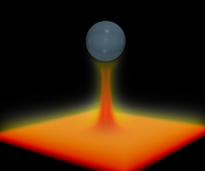
  $500\,\mathrm {mol}\,\mathrm {m}^{-3}$) as the electrolyte. A schematic is provided in figure 1(a) demonstrating the chemical reactions at the cathodic part of the cell. Full dissociation of sulfuric acid to sulphate ( $\mathrm {SO}^{2-}_4$) and hydrogen ( $\mathrm {H}^+$) ions is assumed according to
 \begin{equation} \mathrm{H}_2\mathrm{SO}_{4(aq)} \rightarrow 2\mathrm{H}^+_{(aq)} + \mathrm{SO}_{4(aq)}^{2-}, \end{equation}
and, in order to avoid further complications, self-ionisation of water is disregarded due to its low equilibrium constant at room temperature. The cathodic reactions solely comprise the hydrogen-evolution reaction as
 \begin{equation} 2\mathrm{H}^+ + 2\mathrm{e}^- \rightarrow \mathrm{H}_2, \end{equation}
whereby the hydrogen enrichment and electrolyte depletion co-occur within a mass-transfer boundary layer in the vicinity of the electrode, as schematically illustrated in figure 1(a).

Figure 1. (a) Schematic representation of the two-phase electrochemical system with relevant chemical reactions and boundary conditions at the cathode. (b) Sketch of the three-dimensional numerical set-up with the applied boundary conditions for the velocity field (periodic, no slip (ns), no penetration (np) and free slip (fs)). The bubble is modelled with IBM using a triangulated Lagrangian grid on the bubble interface (a sample is illustrated in (b)). Current density is uniformly distributed on the electrode surface except for an inactive  $(i=0)$ circular part with an outer radius of $R_a=0.75R$ under the bubble.
The numerical set-up is a cuboid box, as depicted in figure 1(b). The electrode is oriented horizontally ( $x$ and $y$ directions) such that the gravitational acceleration $\boldsymbol {g}$ acts normal to it in the negative $z$ direction. A fully spherical hydrogen bubble is initialised with a certain radius ( $R_0=50\,\mathrm {\mu }$m) and zero-degree contact angle on the electrode. The bubble subsequently grows to a prescribed diameter, namely the break-off diameter $d_b$, before it departs from the electrode surface and rises within the electrolyte solution due to its buoyancy. This process then repeats with the next bubble initialised at the same spot as soon as the previous bubble exits from the top boundary. By applying periodicity in the lateral directions of the computational domain, the set-up replicates a system of monodisperse bubbles with uniform spacing of $S=L_x=L_y$ which synchronously grow and rise in the medium. The initialisation, growth and rise of the bubbles in succession are modelled until an equilibrium state is attained, i.e. the averaged mass-transfer statistics, which will be introduced in § 2.3, remain constant in time.
The control parameters for the electrolytically generated two-phase free-convective flow are the cathodic current density  $i$, the bubble break-off diameter $d_b$ and the bubble spacing $S$. Simulations are performed with two different sets of configurations, as listed in table 1; in the first set, the bubble spacing is kept constant while the bubble break-off diameter is varied. In the second set, the spacing between the bubbles is varied at a constant break-off diameter of the bubbles to investigate the effect of bubble population density on the mass transport at the electrode. An auxiliary parameter for either set is the fractional bubble coverage of the electrode, $\varTheta$, which refers to the fraction of the electrode area shadowed by the orthogonal projection of the bubble surface. It is formulated as $\varTheta ={\rm \pi} d_b^2/4A_e$, where $A_e=L_xL_y$ is the electrode area available for a single bubble. At each configuration, 13 current densities within the range $10^1 \le \vert i \vert \le 10^4\,\mathrm {A}\,\mathrm {m}^{-2}$, as listed in table 1, are simulated.
Table 1. Simulation parameters for cases with varying bubble departure diameter  $d_b$ at constant bubble spacing, and with varying bubble spacing $S=L_x=L_y$ at a fixed bubble departure diameter. The domain height is $L_z=4$ mm for all the simulation cases. At each configuration, the simulations are performed at 13 different current densities, as listed in the last column, leading to 130 simulation cases in total.

2.2. Governing equations
2.2.1. Carrier phase
The three-dimensional transient incompressible Navier–Stokes equations in a Cartesian coordinate system are adopted to solve for the velocity field,  $\boldsymbol {u}$, which include the momentum equation
 \begin{equation} \frac{\partial \boldsymbol u}{\partial t} + \boldsymbol{\nabla}\boldsymbol{\cdot} (\boldsymbol{uu}) ={-} \boldsymbol{\nabla} p + \nu \nabla^2 \boldsymbol{u} + \boldsymbol{f_u}, \end{equation}
and the continuity equation
 \begin{equation} \boldsymbol{\nabla}\boldsymbol{\cdot} \boldsymbol{u} = 0. \end{equation}
Here,  $\boldsymbol {\nabla }$ is the gradient operator vector, $p$ is the modified kinematic pressure (i.e. the total pressure with the hydrostatic pressure subtracted) and $\nu$ is the kinematic viscosity of the solution; $\boldsymbol {f_u}$ denotes the direct forcing introduced in the IBM framework in order to enforce the velocity boundary conditions on the bubble interface.
In the most general case, the distribution of the  $\mathrm {H}_2\mathrm {SO}_4$ is obtained by solving the advection–diffusion–migration equation for its constituent ions ( $\mathrm {H}^+$, $\mathrm {SO}^{2-}_4$). However, for a binary electrolyte it is possible to simplify the problem by assuming electroneutrality throughout the electrolyte (Dickinson, Limon-Petersen & Compton Reference Dickinson, Limon-Petersen and Compton2011), thus eliminating the migration terms between the ion transport equations. Hence, a single transport equation for $\mathrm {H}_2\mathrm {SO}_4$ with an effective diffusivity is obtained (Morris & Lingane Reference Morris and Lingane1963; Sepahi et al. Reference Sepahi, Pande, Chong, Mul, Verzicco, Lohse, Mei and Krug2022). Additionally accounting for $\mathrm {H}_2$, the transport of each substance, $C_j$, in the system can be described by an effective advection–diffusion equation as
 \begin{equation} \frac{\partial C_j}{\partial t} + \boldsymbol{\nabla}\boldsymbol{\cdot} (\boldsymbol u C_j)= D_j \nabla^2 C_j + \boldsymbol{f}_{C_j}, \end{equation}
where the subscript  $j=(s, \mathrm {H}_2)$ refers to $\mathrm {H}_2\mathrm {SO}_4$ and $\mathrm {H}_2$, respectively. Here, $\boldsymbol {f}_{C_j}$ is the IBM forcing term to enforce the respective gas–liquid interfacial condition for each substance, which will be explained in § 2.2.2. The effective diffusivity of $\mathrm {H}_2\mathrm {SO}_4$ can be obtained from the mass diffusivities, $D_k$, and ionic valences, $z_k$, of the ions ( $k=1,2$ denotes $\mathrm {H}^+$ and $\mathrm {SO}^{2-}_4$, see table 2 for ions diffusivity) as
 \begin{equation} D_s=\frac{D_1 D_2(z_1 - z_2)}{z_1D_1 -z_2D_2}. \end{equation}
Table 2. Physical properties of the analysed system.

The no-slip impermeable condition is applied on the electrode. A uniform current density,  $i=I/A_e$, where $I$ and $A_e$ are respectively the overall electric current and electrode surface area, is spread on the electrode surface, except for an inactive area with instantaneous radius of $R_a=0.75R$ (Vogt & Stephan Reference Vogt and Stephan2015) underneath the bubble where zero current density is applied ( $R$ is the instantaneous bubble radius, see figure 1b). The current density in the outer region is therefore corrected slightly as the bubble grows in order to keep the overall electric current $I$ constant throughout the simulations. The maximum transient enhancement of the local current density away from the bubble is $1/(1-0.75^2\varTheta )$ just before the bubble departure. The current density is homogeneous across the entire electrode during the rise phase of each bubble. The cathodic set of boundary conditions for $C_j$ reads (Morris & Lingane Reference Morris and Lingane1963; Sepahi et al. Reference Sepahi, Pande, Chong, Mul, Verzicco, Lohse, Mei and Krug2022)
 $$\begin{gather} -\frac{i}{(n_e/s_1)F}=2D_1\left(1-\frac{z_1}{z_2}\right) \left(\frac{\partial C_s}{\partial z}\right)_{z=0}, \end{gather}$$
 $$\begin{gather}\frac{i}{(n_e/s_{\mathrm{H}_2)}F}=D_{\mathrm{H}_2} \left(\frac{\partial C_{\mathrm{H}_2}}{\partial z}\right)_{z=0}. \end{gather}$$
Here,  $n_e=2$ is the number of the transferred electrons in the cathodic reaction (2.2), $s_1=2$ and $s_{\mathrm {H}_2}=1$ are the stoichiometric coefficients of the ions and $F=96\,485\,\mathrm {C}\,\mathrm {mol}^{-1}$ is the Faraday constant. After simplification, the corresponding cathodic flux $J_j=-D_j({\partial C_j}/{\partial z})_{z=0}$ for each species can be related to the current density via the Faraday constant as
 \begin{equation} J_{s}=\frac{1}{3} \frac{i}{F}\frac{D_s}{D_1},\quad \text{and}\quad J_{\mathrm{H}_2}={-}\frac{i}{2F}. \end{equation}
While generally the boundary conditions at the top boundary are free slip no penetration and constant concentrations for the velocity and scalar fields, respectively, a remedy is required to allow the bubble to pass the top boundary. For this purpose, we momentarily change the boundary condition to an in–outflow condition once the bubble arrives at the top boundary and revert back to the original boundary conditions once the bubble has left the computational box. The bubble passes through the top boundary with a constant velocity equal to its rise velocity before the boundary condition switch. We ensured that the computational domain is sufficiently high such that this procedure has negligible influence on mass-transfer processes at the electrode. Moreover, periodic boundary conditions for the velocity and concentration fields are employed in the lateral directions of the computational domain. The choice of these boundary conditions is such that the corresponding pure-diffusion problem, i.e. in the absence of advection, reaches a steady state for which an analytical self-similar solution exists (Carslaw & Jaeger Reference Carslaw and Jaeger1959; van der Linde et al. Reference van der Linde, Moreno Soto, Peñas-López, Rodríguez-Rodríguez, Lohse, Gardeniers, Van Der Meer and Fernández Rivas2017). Thus, the known mass-transfer rate of the pure-diffusion problem can be served as a base system for comparison of the mass-transfer change resulting from the bubbly flows within the electrolyte (see § 3).
In order to numerically obtain the solution of (2.4), (2.3) and (2.5), a second-order accurate central finite-difference scheme is employed for spatial discretisation and time marching is performed with a fractional step third-order accurate Runge–Kutta scheme (Kim & Moin Reference Kim and Moin1985; Verzicco & Orlandi Reference Verzicco and Orlandi1996). A multiple-resolution strategy (Ostilla-Monico et al. Reference Ostilla-Monico, Yang, van der Poel, Lohse and Verzicco2015), with a refinement factor of two for the scalar fields, is used to solve the momentum and scalar equations, to cope with the fact that the mass diffusivity is several orders of magnitudes smaller than the momentum diffusivity. The grid is equally spaced in all directions. A grid independence check has also been performed and is reported in Appendix A.2.
2.2.2. Dispersed phase
Numerically, we represent the growth and rise phases of the bubbles but circumvent the intricacies of the nucleation process by initialising the bubbles with a finite size of  ${R_0=50\,\mathrm {\mu }}$m. Effectively, the liquid previously located at the bubble position is replaced during this step. However, given the minute volume of the bubble at this point, this does not affect the results. During the growth phase, the expansion rate of the bubble is directly related to the diffusive transport of the dissolved gas across the gas–liquid interface which is determined by Fick's law. Balancing the rate of the change of mass within the bubble and the diffusive flux of hydrogen across the interface as
 \begin{equation} \dot{N}_b =\frac{P_0}{\mathcal{R} T_0 } 4{\rm \pi} R^2 \frac{{\rm d} R}{{\rm d} t}= \int_{\partial V} D_{\mathrm{H}_2} \boldsymbol{\nabla} C_{\mathrm{H}_2} \boldsymbol{\cdot} \hat{\boldsymbol{n}}_b \,\mathrm{d} A, \end{equation}
yields the bubble growth rate
 \begin{equation} \frac{\mathrm{d} R}{\mathrm{d} t}=\frac{\mathcal{R} T_0}{P_0} \frac{1}{4{\rm \pi} R^2} \int_{\partial V} D_{\mathrm{H}_2} \boldsymbol{\nabla} C_{\mathrm{H}_2} \boldsymbol{\cdot} \hat{\boldsymbol{n}}_b \, \mathrm{d} A, \end{equation}
where  $\mathcal {R}$, $T_0$ and $P_0$ are the gas universal constant, ambient temperature and pressure, respectively. Here, $R$ is the instantaneous radius of the bubble and $\hat {\boldsymbol {n}}_b$ is the unit normal vector at the surface $\partial V$ of the bubble. We assume here a constant pressure inside the bubble throughout the growth phase, which is valid since, for the range of bubble sizes $R \geq 50\,\mathrm {\mu }$m, the Laplace pressure is negligible compared with the ambient pressure of $P_0 = 1$ bar. We further neglected inertial effects on the pressure inside the bubble. This is confirmed to be appropriate by computing the inertial terms of Rayleigh–Plesset equation $\rho _L(R\dot R +3\dot R ^2/2)$ (Prosperetti Reference Prosperetti1982). For the largest bubble growth rates encountered in our simulations, the corresponding change in the bubble pressure does not exceed 0.2 Pa, which is small compared with $P_0$.
The bubble detaches and rises under the influence of buoyancy in the electrolyte solution after growing to a prescribed departure diameter,  $d_b$. Note that we do not consider a potential bubble growth during the rise phase such that $R = \mathrm {const.}$ in this case. Given the short rise times ( ${\sim }0.1$ s) compared with the residence time of the bubble on the electrode ( ${\sim }1\unicode{x2013}100$ s) for all but the highest current densities and the significantly lower hydrogen concentrations outside the boundary layer at the electrode, this has hardly any effect on our results. The bubble is treated as a spherical rigid particle during the rising phase and its deformation is disregarded owing to its small size ( $d_b < 1\,\mathrm {mm}$), i.e. surface tension forces, which maintain the spherical form of the bubble, are predominant over inertia and drag forces in the ascent (Weber and capillary numbers are significantly lower than unity). We solve for the translational velocity of the bubble, $\boldsymbol u_b$, which we assume to be governed by Newton's second law of motion as
 \begin{equation} \rho_g V_b \frac{\mathrm{d} \boldsymbol u_b}{\mathrm{d} t} =\int_{\partial V_b} \boldsymbol \tau \boldsymbol{\cdot}\hat{\boldsymbol{n}}_b \, \mathrm{d} A + (\rho_G - \rho_L)V_b\boldsymbol{g}, \end{equation}
where
 \begin{equation} \boldsymbol u_b=\frac{\mathrm{d}\kern 0.06em \boldsymbol x_b}{\mathrm{d} t},\quad \boldsymbol \tau ={-}p \boldsymbol{I} + \mu (\boldsymbol{\nabla} \boldsymbol{u} + \boldsymbol{\nabla} \boldsymbol{u}^{\rm T}). \end{equation}
Here,  $\boldsymbol x_b$ is the bubble centroid position, $\rho _G$ and $\rho _L$ are the gas and fluid densities, respectively, $V_b$ is the bubble volume after detachment and $\boldsymbol \tau$ is the stress tensor for Newtonian fluids. A method and validation to integrate (2.12) numerically is discussed in Appendix A.1.
A set of the boundary conditions for the carrier phase on the bubble interface is required for the concentration and velocity fields. Saturation concentration based on Henry's law  $C_{\mathrm {H}_2,sat}=k_hP_0$, with $k_h$ being Henry's constant for $\mathrm {H}_2$ and zero flux $\boldsymbol {\nabla } C_s \boldsymbol {\cdot } \hat {\boldsymbol {n}}_b =0$ for $\mathrm {H}_2\mathrm {SO}_4$, is applied on the bubble interface. Assuming a fully contaminated bubble (Takagi & Matsumoto Reference Takagi and Matsumoto2011), the no-slip no-penetration condition is employed on the bubble interface ( $| \boldsymbol x - \boldsymbol x_b |=R$) such that the velocity $\boldsymbol {u}\vert _{\partial V}$ of a point on the bubble surface is given by
 \begin{equation} \boldsymbol u\vert_{\partial V} = \boldsymbol u_b + \frac{\mathrm{d} R}{\mathrm{d} t} \hat{\boldsymbol{n}}_b. \end{equation}
This relation is coupled to the mass transfer via (2.11) to determine the bubble growth rate  $\mathrm {d} R/\mathrm {d} t$. During the growth stage, we set $\boldsymbol {u}_b = \mathrm {d} R/\mathrm {d} t$ such that the contact point of the bubble on the electrode remains stationary. To ensure continuity within the domain during the bubble growth, the continuity equation needs to be revised by adding a source term in the bubble interior according to
 \begin{equation} \boldsymbol{\nabla}\boldsymbol{\cdot} \boldsymbol u = \phi \frac{3}{R}\frac{\mathrm{d} R}{\mathrm{d} t}, \end{equation}
where  $\phi$ is an indicator function which undergoes a smooth transition from 0 to 1, based on a cut-cell method (Kempe & Fröhlich Reference Kempe and Fröhlich2012) for the cells outside and inside the bubble, respectively. This amendment is necessary for modelling expanding/shrinking boundaries using an incompressible solver with IBM. The same approach has also been adopted in the literature for simulation of flows with evaporating droplets (Lupo et al. Reference Lupo, Niazi Ardekani, Brandt and Duwig2019, Reference Lupo, Gruber, Brandt and Duwig2020). The local velocity field is still entirely divergence free outside the bubble and the non-zero divergence inside the bubble is irrelevant to the flow physics outside due the boundary conditions enforced on the gas–liquid interface. To ensure the global conservation of the mass in the course of the bubble growth, a small but non-zero uniform vertical velocity is prescribed at the top boundary such that the outflow rate equals the expansion rate of the bubble, similar to the simulations of evaporating droplets in wall-bounded turbulent flows using IBM (Lupo et al. Reference Lupo, Gruber, Brandt and Duwig2020).
The bubble interface is discretised using another triangulated Lagrangian grid, as depicted in figure 1(b). The IBM method here is based on the moving least squares approach to conduct the interpolation and distribution of the direct forcing terms between the Eulerian and Lagrangian grids (Liu & Gu Reference Liu and Gu2005; Vanella & Balaras Reference Vanella and Balaras2009; Spandan et al. Reference Spandan, Meschini, Ostilla-Mónico, Lohse, Querzoli, de Tullio and Verzicco2017). The enforcement of the Dirichlet and Neumann conditions on the interface for  $\mathrm {H}_2$ and $\mathrm {H}_2\mathrm {SO}_4$ is performed employing a ghost-cell-based IBM to ensure the conservation of the species (Lu et al. Reference Lu, Das, Peters and Kuipers2018). To validate these procedures, we verified that mass conservation for the hydrogen distribution is fullfilled in our simulations (see Appendix A.3).
2.3. Response parameters
The most basic response parameters relate to the transport of  $\mathrm {H}_2$ away and $\mathrm {H}_2\mathrm {SO}_4$ towards the electrode. Since the respective rates of production and consumption at the electrode, $J_{\mathrm {H}_2}$ and $J_s$, are constant in time, the effective transport is reflected in the resulting surface-averaged concentrations of hydrogen, $\tilde {C}_{\mathrm {H}_2,e}$, and electrolyte, $\tilde {C}_{s,e}$, at the electrode surface. These need to be compared with the respective concentration values in the bulk, for which we adopt the top boundary conditions, which equal the initial values, i.e. $C_{\mathrm {H}_2,0} =0$ and $C_{s,0}$. We then normalise the differences between the concentrations at the electrode and at the top of the domain using the (constant) fluxes $J_j$ and the bubble diameter $d_b$ as reference scales to yield the Sherwood numbers
 \begin{equation} \widetilde{Sh}_{\mathrm{H}_2,e}=\frac{J_{\mathrm{H}_2} d_b}{D_{\mathrm{H}_2} \tilde{C}_{\mathrm{H}_2,e}} \quad \text{and}\quad \widetilde{Sh}_{s,e}=\frac{J_{s}d_b}{D_{s} (C_{s,0} - \tilde{C}_{s,e})}. \end{equation}
Here, and in the following, the tilde symbol is used to mark time-dependent surface-averaged response parameters; corresponding averages over a bubble period appear without a tilde. By introducing the boundary-layer thickness  $\tilde \delta _j=D_j {\rm \Delta} \tilde C_j/J_j$, this Sherwood number can equivalently be expressed as $\widetilde {Sh}_j = d_b/\tilde \delta _j$. For pure diffusion, $\tilde \delta _j$ ultimately reaches the cell height irrespective of the current density such that the same steady-state value of $\widetilde {Sh_j}$ would be obtained for all cases without the effect of the bubbles.
Analogously, we characterise the mass transfer of hydrogen into the bubble using the bubble Sherwood number
 \begin{equation} \widetilde{Sh}_{\mathrm{H}_2,b}=\frac{2\dot R R}{\dfrac{\mathcal{R} T_0}{P_0}D_{\mathrm{H}_2} (\tilde{C}_{\mathrm{H}_2,e}-C_{\mathrm{H}_2,sat})}, \end{equation}
which employs the instantaneous bubble diameter,  $2R$, the surface area, $4{\rm \pi} R^2$, and the concentration difference between the electrode and bubble interface, $(\tilde {C}_{\mathrm {H}_2,e} - C_{\mathrm {H}_2,sat} )$, for normalisation of the mass flux into the bubble given by (2.10).
A final important output is the fraction of the total hydrogen produced that ends up in gaseous form, i.e. gets desorbed into the bubble (Vogt Reference Vogt1984a,Reference Vogtb, Reference Vogt2011a,Reference Vogtb). Mathematically formulating this leads to an expression for the gas-evolution efficiency
 \begin{equation} f_G=\frac{\dfrac{V_b}{\tau_c}}{\dfrac{\mathcal{R} T_0}{P_0}\dfrac{-i}{n_eF}A_e}=\frac{\dot V_G}{\dfrac{\mathcal{R} T_0}{P_0}\dfrac{-i}{n_eF}A_e}, \end{equation}
where  $\tau _c=\tau _g + \tau _r$ is the bubble lifetime, which comprises the bubble residence (growth) time, $\tau _g$, and the bubble rise time, $\tau _r$. Here, $\dot V_G=V_b/\tau _c$ is the volumetric gas flux into the gas phase.
3. Bubble dynamics and mass transfer at the electrode
To begin with, we present the simulation results for a bubble departure diameter of  $d_b=0.5$ mm and spacing $S=2$ mm. The physical properties of the system are set in accordance with table 2. Figure 2(a) shows the growth dynamics of successively generated bubbles on the electrode at four different current densities. At each current density, the first few bubbles show a slower growth while the supersaturation level of the gas in the electrode boundary layer is building up and the growth pattern becomes more repetitive at later times. This is also reflected in the bubble growth time, which drops initially, but remains constant for subsequent bubbles later on (see inset of figure 2b). These observations are indicative of an equilibrium state, in which the time-averaged mass transport and gas production rates at the electrode surface are balanced, leading to the repetition of the same growth dynamics for bubbles evolving in sequence. The bubble size evolution at the statistically steady state is plotted and compared in figure 2(b) for different current densities. These curves have been taken at times when the bubble residence time, $\tau _g$, no longer varies with bubble number $n$, as depicted in the inset. Despite the fact that the bubble growth time varies over several orders of magnitude from 100 s to less than 0.1 s when increasing the current density from $10^1$ to $10^4\,\mathrm {A}\,\mathrm {m}^{-2}$, the growth dynamics pertaining to diffusion-limited growth, i.e. $R~\propto t^{1/2}$, is maintained (Epstein & Plesset Reference Epstein and Plesset1950; Scriven Reference Scriven1959). This is evidenced by the double-logarithmic plot of the bubble size evolution in figure 2(c), where the time axis is normalised with $\tau _g$. In this form, all cases approximately collapse onto a single curve that is in good agreement with the $1/2$ power law.

Figure 2. (a) Radius of the successively growing bubbles as a function of time for current densities  $\lvert i \lvert =10^1,10^2,10^3$ and $10^4\,\mathrm {A}\,\mathrm {m}^{-2}$. The radius has been normalised with the initial size of the bubble used for the simulations, $R_0=50\,\mathrm {\mu }$m. (b) Temporal evolution of the bubble radius at the statistically steady state for each current density in the range of $10^1<\lvert i \lvert <10^4\,\mathrm {A}\,\mathrm {m}^{-2}$. The magnitude of the current density is illustrated with the colour map. Here, $t_0$ is the start of the bubble lifetime in each case and hence $t_g=t-t_0$ is the bubble age. The inset shows the bubble growth time, $\tau _g$, for the $n$th bubble. (c) Double-logarithmic plot of the bubble-evolution curve for all the current densities. Time axis has been normalised with the growth time in the steady state, as shown in the inset of (b).
Next, we look into the mass-transfer rate at the electrode by tracking the spatially averaged concentrations on the electrode surface in time, as shown in figures 3(a) and 3(b) for  $\mathrm {H}_2$ and $\mathrm {H}_2\mathrm {SO}_4$, respectively. As the reaction proceeds, the hydrogen concentration increases in time in contrast to the electrolyte concentration, which is depleted at the electrode. For the one-dimensional pure-diffusion problem in the absence of the bubbles (diffusion in a semi-infinite medium with constant flux on the boundary) the analytical solution gives the time evolution of the cathodic concentrations, $\tilde {C}^{\ast }_{j,e}$, as (Bejan Reference Bejan1993)
 \begin{equation} \tilde{C}^{*}_{j,e}(t)-C_{j,0}=2J_j \sqrt{\frac{t}{{\rm \pi} D_j}}, \end{equation}
which has been provided for comparison at each current density in figures 3(a) and 3(b). Small differences between this solution and the simulation results are related to the presence of the adhering bubble on the electrode and the inactive area underneath it, which alters the local concentrations slightly. Major deviations from the analytical solution occur after the departure of the first bubble, which leads to significantly enhanced mixing. As a result, fresh electrolyte is transported to the electrode, replacing the gas-enriched and electrolyte-depleted solution there. Eventually, the system reaches an equilibrium in which the reaction and transport rates are balanced, such that the cycle-averaged concentrations remain constant in time.

Figure 3. Temporal evolution of hydrogen (a) and electrolyte (b) averaged concentrations at the electrode surface for bubble departure diameter of  $d_b=0.5$ mm and spacing of $S=2$ mm for all the investigated current densities. Broken black lines represent the solution of the pure-diffusion problem in a semi-infinite medium with constant flux condition at the boundary, calculated using (3.1). Corresponding Sherwood numbers of simulations and pure-diffusion problem for hydrogen (c) and electrolyte (d) transport computed based on (2.16a,b). Insets in (c,d) show a closer view of Sherwood variation for the highest current density in the statistically steady state. Current density at each case is distinguished using the colour map whose range is shown in the colour bar.
A comparison of the behaviour for different current densities  $i$ is best done using the transient Sherwood numbers (2.16a,b) plotted in figures 3(c) and 3(d) for $\mathrm {H}_2$ and $\mathrm {H}_2\mathrm {SO}_4$, respectively. Prior to the first bubble departure from the electrode surface, time-dependent Sherwood numbers collapse to a single curve regardless of the current density, as do those pertaining to the analytical solution of the pure diffusion problem. The bifurcation from the main trend happens after the detachment of the first bubble, i.e. transition to the convection, which takes place earlier at higher current density due to the higher oversaturation of the dissolved gas in the electrode boundary layer and faster bubble growth. Once the system is at equilibrium and the bubble generation rate no longer changes, the Sherwood numbers also approach an equilibrium value. Small oscillations around this value occur within each bubble cycle (see insets for the highest current density). For these, the minima of $\widetilde {Sh}_{j,e}$ correspond to the detachment times after which the Sherwood numbers immediately increase and the maxima are the instants when the bubble lifetime starts, followed by a slow decrease during the growth time. Furthermore, due to the higher frequency of bubble generation and hence stronger mixing in the electrolyte, the effective mass-transfer rate at the electrode, reflected in the values of $\widetilde {Sh}_{j,e}$ in equilibrium, is significantly enhanced at higher current densities.
In order to provide insight into the flow structure and scalar distribution in the equilibrium state, figure 4 displays snapshots of the hydrogen supersaturation,  $\zeta _{\mathrm {H}_2}=C_{\mathrm {H}_2}/C_{\mathrm {H}_2,sat}-1$, overlaid with velocity vectors at different stages of the bubble evolution and for varying current densities. For the case with $\vert i \vert =10^3\,\mathrm {A}\,\mathrm {m}^{-2}$, corresponding plots for the electrolyte concentration distribution are provided in figure 5. At this current density, a maximum electrolyte depletion of ${\approx }15\,\%$ occurs at the electrode and, even in the most extreme case with $\vert i \vert =10^4\,\mathrm {A}\,\mathrm {m}^{-2}$, this value does not exceed ${\approx }70\,\%$, meaning that the electrolyte concentration remains finite in all cases even though the diffusion-limited current density, $\vert i \vert _{diff} = n_e F D_s C_{s,0}/L_z = 59.7\,\mathrm {A}\,\mathrm {m}^{-2}$, is exceeded significantly. The associated transport enhancement is due to a large-scale convective pattern that is established during the rise stage, with an up-draught stream in bubble column, downwelling flow along the (periodic) sidewalls and wall-parallel flow close to the electrode. At low current density (figure 4a), the bubble driving is highly intermittent as the convective motion dissipates during the long growth period. However, as the latter becomes shorter for larger $i$ (figures 4(b) and 4(c)), the flow becomes more and more continuous and a strong circulation is visible throughout the entire bubble cycle at $\vert i \vert = 10^4\,\mathrm {A}\,\mathrm {m}^{-2}$ in figure 4(d). The convective pattern counteracts the penetration of the electrode boundary layer into the bulk by advecting the fresh electrolyte towards the electrode. This effect is stronger at higher currents due to the higher frequency of bubble formation driving a stronger flow. This can be also appreciated from figures 6(a) and 6(b), which compare the vertical profiles of normalised $\mathrm {H}_2$ and $\mathrm {H}_2\mathrm {SO}_4$ at a location half-way between adjacent bubbles, where an appreciable drop in the electrode boundary layer thickness with increasing current density is observed, consistent with an enhanced mass transport.

Figure 4. Snapshots of the hydrogen and velocity distributions in the equilibrium state at different stages of the bubble lifetime for current densities of (a)  $10^1$, (b) $10^2$, (c) $10^3$ and (d) $10^4\,\mathrm {A}\,\mathrm {m}^{-2}$. Bubble break-off diameter is $d_b=0.5$ mm and spacing is set at $S=2$ mm. In all cases, the first three images cover the bubble growth and the last three the bubble rise time. The supersaturation level, $\zeta _{\mathrm {H}_2}$, is shown using the colour bar. The superimposed vectors represent the induced velocity field by the growth and rise of the bubbles in the electrolyte. The velocity scale provided at the right of the figure applies to all panels.

Figure 5. Snapshots of the electrolyte distribution for the case ( $\vert i \vert =10^3\,\mathrm {A}\,\mathrm {m}^{-2}$) shown in figure 4(c).

Figure 6. Vertical profiles of normalised hydrogen (a) and electrolyte (b) concentration half-way between adjacent bubbles (see the sketch in (a)) at the instant of bubble break-off. The profiles are captured at the statistically steady state for different current densities.
3.1. Current dependence of the Sherwood number and bubble size effect
Next, we consider the current dependence of the Sherwood numbers of hydrogen and electrolyte transport, averaged over an entire bubble lifetime in the statistically steady state, which are plotted in figure 7(a,b), respectively. Apart from the case with  ${d_b = 0.5\ \textrm{mm}}$ considered so far, these panels also include results for other bubble departure diameters. The trend of increasing $Sh_j$ with increasing $i$, which was already evident in figure 3(c,d) for $d_b = 0.5$ mm, is consistently observed for all these cases. The current dependence approximates a power-law scaling of $Sh_j \sim i^{1/3}$, especially for larger bubbles, but deviations occur for smaller bubbles at high current densities, where $Sh_j$ increases significantly slower. It is further interesting to examine how $Sh_{\mathrm {H}_2,e}$ and $Sh_{{s,e}}$ relate to each other, which we do by plotting the ratio $Sh_{{s,e}}/Sh_{\mathrm {H}_2,e}$ in figure 7(c). Given that $Sh_{{s,e}}/Sh_{\mathrm {H}_2,e} = \delta _{\mathrm {H}_2}/\delta _s$, one expects this ratio to yield a constant of either $( D_{\mathrm {H}_2}/D_s)^{1/2}$ (for diffusive transport) or $(D_{\mathrm {H}_2}/D_s)^{1/3}$ (for convection given that the Schmidt number $Sc_j = D_j/\nu$ is large (Bejan Reference Bejan1993)) for a single-phase flow. In the present simulations, $D_{\mathrm {H}_2}/D_s =1.5$, such that the resulting values (1.22 and 1.14) do not differ significantly. In our results in figure 7(c), a ratio of comparable magnitude is attained for the smallest bubbles and similar values are also approached for the cases with larger $d_b$ at successively larger magnitudes of $i$. The deviation from the single-phase value is related to the fact that the electrolyte is only transported in solution while hydrogen is also carried inside the bubble. It is therefore most pronounced at low current densities and for large bubble sizes since, for these cases, the fraction of gas transported in the bubbles is largest as the plot of $f_G$ in figure 8(a) confirms. The gas efficiency decreases significantly with decreasing bubble size, but is only a weak function of the current density, especially for $i\lessapprox 10^3\,\mathrm {A}\,\mathrm {m}^{-2}$. From the gas-evolution efficiency relation (2.18), it is deduced that $\tau _g \sim V_b (f_Gi)^{-1}$, considering a constant rise time ( $\tau _c$) for bubbles with the same size. Given the weak dependence of $f_G$ on $i$, the scaling of $\tau _g/V_b \sim i^{-1}$ holds reasonably well for all the cases shown here, as can be seen from figure 8(b).

Figure 7. Sherwood number of (a) hydrogen and (b) electrolyte transport averaged over an entire bubble lifetime in the statistically steady state, as a function of current density for different bubble break-off diameters,  $d_b$. The broken lines indicate the power-law relation $Sh_j \sim i^{1/3}$ for reference. (c) Ratio of electrolyte to hydrogen Sherwood numbers vs the current density at different bubble diameters. Dashed and dashed-dotted lines correspond to $(D_{\mathrm {H}_2}/D_s)^{1/3}$ and $(D_{\mathrm {H}_2}/D_s)^{1/2}$, respectively, for comparison.

Figure 8. (a) Gas-evolution efficiency,  $f_G$, as a function of current density for different bubble break-off diameters, $d_b$. (b) Bubble residence time, $\tau _g$, compensated with bubble departure volume, $V_b$, as a function of current density for different values of $d_b$. The broken line indicates the power law of $\tau _g \sim i^{-1}$.
3.2. Effect of bubble spacing
Changing the bubble departure size, as was done in § 3.1, has multiple effects since it affects bubble growth times and the flow, but also alters the effective bubble coverage  $\varTheta$. To disentangle these, we now fix the departure diameter of the bubble at $d_b=0.5$ mm and vary the box size $S$ to explore a range of $0.02 \le \varTheta \le 0.56$. This resembles a change in the bubble population density, which in practice is tied to the current density and typically increases when $i$ is increased (Vogt & Balzer Reference Vogt and Balzer2005; Vogt Reference Vogt2013). Taking advantage of the numerical simulations, we can explore the effect of this parameter independently here.
Figures 9 and 10 offer insight into how changing  $\varTheta$ affects the mass-transport processes at the electrode by showing snapshots of the distributions of $\mathrm {H}_2$ and $\mathrm {H}_2\mathrm {SO}_4$, respectively, taken in the instant of bubble detachment after the system has reached a steady state. Figure 9(a) displays data for $\mathrm {H}_2$ at the lowest current density investigated ( $\vert i \vert = 10^1\,\mathrm {A}\,\mathrm {m}^{-2}$). For this case, the boundary layers are thick due to the weak convective transport at low $\varTheta$. However, as the bubble coverage is increased, the amount of dissolved hydrogen decreases and almost all the produced gas is contained in the bubble at $\varTheta = 0.56$. This implies very efficient transport for $\mathrm {H}_2$ via the gas phase, but since the detachment frequency is low, the same does not hold for $\mathrm {H}_2\mathrm {SO}_4$, as can be seen from figure 10(a). Here, the depletion boundary layer is very thick, with almost a linear gradient across the domain height. At the highest current density of $\vert i \vert = 10^4\,\mathrm {A}\,\mathrm {m}^{-2}$, the significantly shorter detachment period leads to a much stronger driving of the flow. Convective transport therefore prevails even at high $\varTheta$, where $\tau _c$ tends to increase as the amount of hydrogen produced per bubble decreases for smaller bubble spacings (see figure 12c). As a consequence, not only the hydrogen boundary layer (figure 9b) but also that for the electrolyte concentration (figure 10) remains thin, even at $\varTheta = 0.56$.

Figure 9. Snapshots of hydrogen supersaturation taken at the time of bubble detachment in the statistically steady state for  $\vert i \vert =10^1$ (a) and $\vert i \vert =10^4\,\mathrm {A}\,\mathrm {m}^{-2}$ (b). The fractional bubble coverage is increased from left to right within the range $0.02 \le \varTheta \le 0.56$ whose value is specified at top. The velocity scale applies to all panels.

Figure 10. Snapshots of normalised  $\mathrm {H}_2\mathrm {SO}_4$ distribution at the time of bubble detachment in the statistically steady state for $\vert i \vert =10^1$ (a) and $10^4\,\mathrm {A}\,\mathrm {m}^{-2}$ (b).
The trends observed in figures 9 and 10 are also reflected in the Sherwood numbers of  $\mathrm {H}_2$ and $\mathrm {H}_2\mathrm {SO}_4$ plotted in figures 11(a) and 11(b). Here, $Sh_{\mathrm {H}_2,e}$ increases with $\varTheta$ throughout the whole range of current densities investigated. Again, the data generally approximate an $i^{1/3}$ scaling, albeit with significant deviations at low $i$ and high $\varTheta$, where the results significantly exceed this trend. Additionally, $Sh_{\mathrm {H}_2,e}$ falls below the $1/3$-scaling line for large current densities and low bubble coverage, which is in accordance with the trend observed in figure 7(a) for smaller $d_b$ for which the value of $\varTheta$ is also reduced. For these higher currents, $Sh_{{s,e}}$ behaves similar to $Sh_{\mathrm {H}_2,e}$ and this is also reflected in the ratio $Sh_{{s,e}}/Sh_{\mathrm {H}_2,e}$ (figure 11c) being close to those expected for single-phase transport. Interestingly, $Sh_{{s,e}}/Sh_{\mathrm {H}_2,e}$ attains values even slightly larger than 1.22 for larger $\varTheta$. Presumably, this is caused by the lower $\mathrm {H}_2$ concentration in the dissolved phase, which dominates the transport for these cases. Remarkably, the $\varTheta$ trend of $Sh_{{s,e}}$ at current densities $\vert i \vert \lessapprox 10^3\,\mathrm {A}\,\mathrm {m}^{-2}$ is opposite to that observed for the hydrogen transport in this regime with $Sh_{{s,e}}$ decreasing for larger $\varTheta$. The ratio $Sh_{{s,e}}/Sh_{\mathrm {H}_2,e}$ drops to values as low as 0.1 for the most extreme case, confirming that the gas is predominantly carried in bubbles whose rise triggers no significant convection as the detachment frequency is low.

Figure 11. Sherwood number of (a) hydrogen and (b) electrolyte transport averaged over one bubble lifetime in the statistically steady state, as a function of current density for different bubble spacings. The bubble departure diameter is fixed at  $d_b=0.5$ mm and the range of fractional bubble coverage is $0.02 \le \varTheta \le 0.56$, as specified in the legend.
Corresponding results for the gas-evolution efficiency,  $f_G$, are presented in figure 12(a). As expected, $f_G$ increases significantly with fractional bubble coverage, $\varTheta$. It approaches unity at lower currents and for the tightest spacings, consistent with the observations in figures 9(a) and 11(c). Furthermore, $f_G$, generally decreases at higher current densities because the more frequent detachment events drive an increasingly stronger convection. As a result, the bulk of the gas is transported in dissolved form at $\vert i \vert = 10^4\,\mathrm {A}\,\mathrm {m}^{-2}$ even at the highest coverage of $\varTheta = 0.56$. When comparing our data with the empirical relation provided by Vogt (Reference Vogt2011b), it is important to keep in mind that, in practice, increasing current density generally leads to higher $\varTheta$. To identify realistic combinations of $i$ and $\varTheta$ in the simulations, we compare the parameter space with the $\varTheta (i)$-relation given by Vogt & Balzer (Reference Vogt and Balzer2005) in figure 12(c). Simulations lying close to this line are marked with filled symbols in figure 12(a–c). When considering these data points only, our results for $f_G$ in figure 12(a) approximately agree with the empirical relation for $\vert i \vert \sim 10^3\,\mathrm {A}\,\mathrm {m}^{-2}$, but differences arise for higher and in particular for low current densities $\vert i \vert \leq 10^2\,\mathrm {A}\,\mathrm {m}^{-2}$.

Figure 12. (a) Gas-evolution efficiency,  $f_G$, as a function of current density for varying bubble spacings (specified in terms of the fractional bubble coverage, $\varTheta$). The bubble departure diameter has been fixed at $d_b=0.5$ mm. (b) Gas-evolution efficiency vs bubble coverage for varying current densities. (c) Hydrogen supersaturation on the electrode surface, $\zeta _{\mathrm {H}_2,e}$, for all the simulation cases with varying current density and bubble spacing. (d) Bubble lifetime, $\tau _c$, premultiplied with current density as a function of bubble coverage for varying current densities. The relevant empirical relations by Vogt et al. are provided with broken lines in the panels. The filled markers in (a,b) show the closest data to the empirical relation $\varTheta =0.023 \vert i\vert ^{0.3}$ (Vogt & Balzer Reference Vogt and Balzer2005) in (c), to highlight the more realistic cases.
The results for  $f_G$ are replotted in figure 12(b), but this time as a function of $\varTheta$ since this is the practically more relevant form. It also allows for a comparison with the relations provided by Vogt (Reference Vogt2011b, Reference Vogt2013), Vogt & Stephan (Reference Vogt and Stephan2015) and Vogt (Reference Vogt2017) based on theoretical considerations (see dashed grey and green lines in figure 9b). An obvious difference is that empirical relations are independent of $i$, whereas the data at any given $\varTheta$ exhibit a significant variation depending on the current density. This difference is significantly less prominent when considering only the ‘realistic’ cases. This implies that the change in $\varTheta$ approximately accounts for the dependence on $i$ within this subset. Results for the ‘realistic’ parameter combinations are also reasonably well approximated by the expression of Vogt (Reference Vogt2017), at least up to $\varTheta \approx 0.3$.
Figure 12(c) also includes results for the hydrogen supersaturation on the electrode in the steady state,  $\zeta _{\mathrm {H}_2,e}$, which are shown as colour contours interpolated between the simulation data points. Remarkably, the ‘realistic’ cases close to the relation of Vogt & Balzer (Reference Vogt and Balzer2005) are seen to cover a very wide range of $\zeta _{\mathrm {H}_2,e} \approx 10$ up to very high values exceeding $10^3$. It should be noted, however, that for the latter cases, the boundary layers are very thin (see figure 9b), such that the effective supersaturation on the scale of the bubble will be significantly lower.
As a final point, we plot the bubble lifetime,  $\tau _c$, in figure 12(d). To compensate for the $1/i$-dependence, which leads to variations in $\tau _c$ over 4 orders of magnitude, the data are premultiplied by $i$. For $f_G = \textrm {const.}$, all curves in the presented form would be expected to collapse onto a single line with linear dependence on $\varTheta$ based on (2.18). While the linear trend is approximately preserved for all but the highest current density, the variations in $f_G$ lead to an increase in $i\tau _c$ with $i$ that is most pronounced for the highest current densities.
3.3. Relating the electrode mass transfer to the effective buoyancy driving
The goal of this section is to provide scaling relations for the mass transport at the electrode based on the relevant physical transport mechanism. Our results so far have already highlighted the relevance of the convective flow driven by the departing bubbles. There is an analogy between the present configuration and single-phase buoyancy-driven convection in the sense that the detaching bubbles resemble the plumes of buoyant liquid in the latter case (Climent & Magnaudet Reference Climent and Magnaudet1999). Analyses based on boundary-layer theory for convective heat transfer along vertical plates yield the power-law dependence on the Rayleigh number  $Ra^{m}$, where the exponent $m$ asymptotically varies from $1/4$ for laminar flows to $1/3$ for turbulent flows at high $Ra$ (Churchill & Chu Reference Churchill and Chu1975). The same power laws have empirically been shown to be valid for the convective heat transfer over horizontal plates and in particular for single-phase free-convective mass transfer over upward-facing horizontal electrodes by Wragg (Reference Wragg1968). Beyond the laminar regime featuring an exponent of $0.25$, these authors provided the relation
 \begin{equation} Sh=0.16 (Gr Sc)^{0.33}, \end{equation}
for the mass transport in the turbulent regime, where the Grashof number  $Gr$ captures the buoyancy forcing and the Schmidt number is given by $Sc=\nu /D$. For two-phase buoyancy-driven convection, $Gr$ can be defined to account for the effective buoyancy provided by the bubbles according to
 \begin{equation} Gr=\frac{gd_b^3}{\nu^2} \frac{\rho_L - \rho_e}{\rho_e}=\frac{gd_b^3}{\nu^2} \frac{\rho_L - [(1-\epsilon)\rho_L+\epsilon\rho_G]}{(1-\epsilon)\rho_L+\epsilon\rho_G}, \end{equation}
where  $\rho _L$ is the density of the bulk electrolyte, $\rho _e$ is the mixture density at the electrode surface, $\rho _G$ is the gas density and $\epsilon$ is the gas volume fraction. Considering $\rho _G \ll \rho _L$ yields the simplified expression
 \begin{equation} Gr=\frac{gd_b^3}{\nu^2}\frac{\epsilon}{1-\epsilon}. \end{equation}
Based on the fact that a single bubble is contained in a box with base area  $A_e$ and height $u_b \tau _c$, where $u_b$ denotes the bubble rise velocity, the gas volume fraction $\epsilon$ can be related to the volumetric flow rate of the gas, $\dot {V}_G=V_b/\tau _c$, by (Zuber Reference Zuber1963)
 \begin{equation} \epsilon=\frac{\dot{V}_G}{A_e u_b}. \end{equation}
For all cases investigated here we find that  $\epsilon \ll 1$. Assuming Stokes drag for the bubbles with a no-slip interface yields the terminal velocity
 \begin{equation} u_b=\frac{1}{18}\frac{gd_b^2}{\nu}\frac{\rho_L - \rho_G}{\rho_L}, \end{equation}
which, along with (2.18), leads to the final expression for  $Gr$ as
 \begin{equation} Gr=18 f_G d_b \frac{i}{n_eF}\frac{\mathcal{R} T_0}{P_0\nu}. \end{equation}
The ratio of buoyancy to viscous forces therefore depends linearly on the input parameters  $d_b$, $f_G$, and in particular on $i$. Consequently, the experimentally reported scaling of $Sh \sim i^{1/3}$ (Janssen & Hoogland Reference Janssen and Hoogland1973; Janssen Reference Janssen1978; Janssen & Barendrecht Reference Janssen and Barendrecht1979; Whitney & Tobias Reference Whitney and Tobias1988) is equivalent to $Sh \sim Gr^{1/3}$, provided that the product of the other two parameters ( $d_b$ and $f_G$) in (3.7) ( $d_bf_G$) remains approximately constant with $i$.
$i$.
Next, we consider the dependence of the Sherwood numbers for the mass transport at the electrode on  $Gr$. Figure 13(a) presents a plot of $Sh_{\mathrm {H}_2,e}$ vs $Gr$ for all data presented in §§ 3.1 and 3.2. In this form, the results very convincingly collapse onto a single line, indicating the power law of $Sh_{\mathrm {H}_2,e} \sim Gr^{1/3}$, which supports the adoption of the single-phase concept in the present configuration. Remarkably, the ‘turbulent’ scaling exponent of 1/3 applies to the full range of $Gr$ studied here, even though the flow is relatively weak and only intermittent in some cases (see figures 4 and 9). The data in figure 13(a) are well described by the fit
 \begin{equation} Sh_{\mathrm{H}_2,e}=0.9(Gr Sc_{\mathrm{H}_2})^{1/3}, \end{equation}
where the difference in the prefactor compared with the single-phase equivalent (3.2) is related to the multiphase nature of the present flow but also to the fact that a different length scale of bubble diameter is used here instead of the lateral length scale of the electrode by Wragg (Reference Wragg1968). The only significant deviation from (3.8) occurs for the ‘slow’ (in terms of  $\tau _c$) cases featuring a high $f_G$, for which the gas transport (carried almost exclusively inside the bubbles) is more efficient than buoyancy driving would suggest.

Figure 13. (a) Sherwood number of hydrogen transport,  $Sh_{\mathrm {H}_2,e}$ (2.16a,b), averaged over one bubble lifetime in the statistically steady state, vs $Gr$ for all cases studied in this work. (b) Fractional Sherwood number of hydrogen transport as dissolved gas in the liquid phase, $(1-f_G)Sh_{\mathrm {H}_2,e}$. (c) Corresponding values of $f_G$ vs $Gr$.
$Gr$.
It is important to note that, here,  $Sh_{\mathrm {H}_2,e}$ and therefore (3.8) accounts for the transport of both gaseous and dissolved hydrogen. We can focus on the dissolved transport specifically by multiplying $Sh_{\mathrm {H}_2,e}$ with $(1-f_G)$, as is done in figure 13(b). For reference, a plot of $f_G$ for all data vs $Gr$ is also included in figure 13(c). Consistent with the fact that there is a wide spread in $f_G$ at any given $Gr$, there is no collapse of the data in figure 13(b), underlining that the analogy between single and multiphase buoyancy-driven flows is applicable at the level of the total transport only.
The transport of the electrolyte, which entirely acts as a passive scalar here, for the most part falls in line with the trends discussed for  $Sh_{\mathrm {H}_2,e}$. In particular, $Sh_{{s,e}}$ primarily follows the power law of $Sh_{{s,e}} \sim Gr^{1/3}$ even with the same prefactor when accounting for the difference in $Sc$, as shown in figure 14(a). However, in accordance with figures 7(c) and 11(c), $Sh_{{s,e}}$ drops below this scaling at low $Gr$ and high $\varTheta$. This means that electrolyte transport from the bulk to the electrode surface is limited when the bubbles highly cover the electrode surface and adhere to it for a long period during their lifetime. According to Vogt (Reference Vogt1989, Reference Vogt2012), a factor contributing to the lower transport of the electrolyte is the blockage effect due to the presence of the bubble, as can be seen from the snapshots in figure 10(a). To account for this, we divide $Sh_{{s,e}}$ by the factor $( 1- \varTheta \tau _g/\tau _c)$ in figure 14(b). Here, $1-\varTheta$ is the fraction of the electrode not covered by the bubble and the additional time scale ratio accounts for the fact that the blockage applies only during the growth time $\tau _g$. Introducing this correction in fact reduces the deviations at lower $Gr$ somewhat (but not fully) and the effect may therefore be relevant in this regime. However, the data for $Gr \gtrapprox 1$ are overcompensated. In summary, it therefore appears that the fact that no sustained convection exists at high bubble coverages if $Gr$ is low plays the most important role leading to the lower electrolyte transport. This leads to limitation in the applicability of the single-phase analogy for this case. Nevertheless, it is worth noticing that the agreement with the 1/3 scaling law is much better for $Sh_{{s,e}}$ (figure 14a) than for dissolved $\mathrm {H}_2$ (figure 13b), even though transport is exclusively within the electrolyte in both cases.

Figure 14. (a) Sherwood number of electrolyte transport,  $Sh_{{s,e}}$ (2.16a,b), averaged over one bubble lifetime in the statistically steady state, vs $Gr$ (3.3) for all cases studied in this work. (b) Value of $Sh_{{s,e}}$ compensated for net blockage effect, $\varTheta \tau _g/\tau _c$, caused by bubbles adhering to the electrode surface in the residence time. The legend specifies cases simulated for different bubble diameters and spacings using the corresponding fractional bubble coverage of the electrode, $\varTheta$. The broken lines indicate the fitted power law, $Sh_{{s,e}} = 1.0 (Gr Sc_{s})^{1/3}$, in which $Sc_{s}=\nu /D_s$.
4. Mass transfer to the bubble
4.1. Bubble growth regimes
We now consider the dynamics of bubble growth and mass transfer into the bubble in more detail. The growth of the electrolytically generated gas bubbles can be approximated by an effective power law of
 \begin{equation} R(t)=\mathcal{B} t^x. \end{equation}
The limiting cases are as follows: during the very initial stage, when the growth of the bubble is strongly influenced by the inertia forces from the liquid (Slooten Reference Slooten1984), an exponent of  $x=1$ has been reported (Westerheide & Westwater Reference Westerheide and Westwater1961; Glas & Westwater Reference Glas and Westwater1964; Brandon & Kelsall Reference Brandon and Kelsall1985; Bashkatov et al. Reference Bashkatov, Hossain, Mutschke, Yang, Rox, Weidinger and Eckert2022). For later times, depending on whether the bubble growth is limited by the diffusive mass transfer of dissolved gas to the interface (Epstein & Plesset Reference Epstein and Plesset1950; Scriven Reference Scriven1959; Westerheide & Westwater Reference Westerheide and Westwater1961) or by the gas production rate in the reaction (Darby & Haque Reference Darby and Haque1973; Verhaart, de Jonge & van Stralen Reference Verhaart, de Jonge and van Stralen1980; Yang et al. Reference Yang, Karnbach, Uhlemann, Odenbach and Eckert2015; Bashkatov et al. Reference Bashkatov, Hossain, Mutschke, Yang, Rox, Weidinger and Eckert2022; Higuera Reference Higuera2022), exponents of $x=1/2$ or $x=1/3$ have been identified, respectively. However, in general, the effective value of the exponent in (4.1) deviates from these values due to the interplay between inertia, diffusion and reaction rates.
Figure 15 presents different growth dynamics in the statistically steady state, depending on current density and bubble coverage. Plotting the bubble radius vs the number of hydrogen moles,  $n_{\mathrm {H}_2}$, produced in the reaction from the beginning of the bubble's lifetime, $t_g$, allows for easy comparison of the bubble growth dynamics over time for the full range of the current density. It is worth noting that $n_{\mathrm {H}_2}=J_{\mathrm {H}_2}A_e t_g$ and therefore $n_{\mathrm {H}_2} \sim i t_g$. Power laws with exponent $1/3$ and $1/2$ have been added for comparison in figure 15 at different bubble coverages. Here, corrections are fitted to the prefactor $\beta =(3\mathcal {R} T_0/4{\rm \pi} R_0^3 P_0 )^{1/3}$, which represents the value for purely reaction-limited growth (i.e. $f_G = 1$). For the lowest bubble coverage in figure 15(a), the growth dynamics is best described by the exponent of $x=1/2$ at all current densities. This indicates that the rate of mass transfer to the bubble is controlled by the diffusive transfer of dissolved hydrogen to the bubble interface for these cases. However, a switch from $x=1/2$ to $1/3$ is appreciable as the current density increases at higher bubble coverages of $\varTheta =0.25$ and 0.40, as presented in figures 15(b) and 15(c). At first sight, it may seem counter-intuitive that the reaction rate becomes more relevant as a limiting factor when it is increased. However, as discussed in the previous section, an increase in current density also significantly intensifies the convective transport, which is then predominantly in the dissolved phase even at high $\varTheta$. This reduces the boundary-layer thickness and the amount of dissolved $\mathrm {H}_2$ (see figures 4 and 9), such that diffusive transport becomes increasingly less relevant compared with the faster reaction rate. Therefore, the exponent approaches $x=1/3$ and the prefactor approaches $\beta$, as observable form figures 15(b) and 15(c) where the bubble size evolution is better described by such power law at higher bubble coverages and current densities.

Figure 15. Temporal evolution of normalised bubble radius,  $R/R_0$, vs the molar amount of hydrogen produced in the cathodic reaction, $n_{\mathrm {H}_2}=J_{\mathrm {H}_2} A_e t_g$, where $t_g$ is the time elapsed from the start of the bubble life in the stationary steady state. The results are for all the investigated current densities (distinguished with the colour map) at bubble coverages of $\varTheta =0.05$ (a) $\varTheta =0.25$, (b) and $\varTheta =0.40$ (c). The second row (d,e) shows the same data as in (a–c) but with logarithmic scaling. The green and black broken lines show the power laws with exponents of $1/3$ and $1/2$, respectively. The prefactors for the 1/3 power law are adjusted relative to the growth constant of purely reaction-limited bubble growth, $\beta =3.6\,\mathrm {nmol}^{-1/3}$.
4.2. Quantification of mass transport to the bubble
Figure 16(a) shows the transient behaviour of  $Sh_{\mathrm {H}_2,b}$ according to (2.17) over one bubble lifetime in the statistically steady state for varying current densities. Since bubble growth is neglected during the rise stage (see § 2.2.2 for further details), $Sh_{\mathrm {H}_2,b}$ becomes equal to zero after the bubble break-off from the electrode surface. In figure 16(a), it can be observed that, at low current densities, an equilibrated mass-transfer rate to the bubble is established towards the end of the bubble residence time. This is evident from nearly constant values of $Sh_{\mathrm {H}_2,b}$ at late stages of the growth phase, for current densities $\vert i \vert < 10^3\,\mathrm {A}\,\mathrm {m}^{-2}$. In contrast, at higher current densities, $Sh_{\mathrm {H}_2,b}$ remains in a transient all the way until the departure of the bubble. To study the mass transport to the bubble, the instantaneous $\widetilde {Sh}_{\mathrm {H}_2,b}$ is averaged over the bubble residence time, $\tau _g$. The corresponding results for the data presented in figure 16(a) are shown in figure 16(b) and indicate an increase of $Sh_{\mathrm {H}_2,b}$ with increasing current density.

Figure 16. (a) Temporal evolution of the Sherwood number for the bubble,  $\widetilde {Sh}_{\mathrm {H}_2,b}$ (2.17), during the entire bubble lifetime, $\tau _c$, in the statistically steady state and across the entire range of current density distinguished using the colour map. The data correspond to the case with bubble departure diameter of $d_b=0.5$ mm and a bubble spacing of $S=2$ mm, which leads to bubble coverage of $\varTheta =0.1104$. (b) The corresponding averaged (over the bubble residence time $\tau _g$) Sherwood number of the bubble, $Sh_{\mathrm {H}_2,b}$, over the residence time, $\tau _g$, plotted against the current density.
To gain a broader understanding of hydrogen transport to the bubble and facilitate its quantification, we have plotted  $Sh_{\mathrm {H}_2,b}$ against current density in figure 17(a) for all the simulation cases, including those with variable bubble size or spacing. It is evident that, at low current densities, $Sh_{\mathrm {H}_2,b}$ is nearly constant and then it starts to ramp up with current density for all of the simulated cases. Furthermore, the lower values of $Sh_{\mathrm {H}_2,b}$ at higher $\varTheta$ suggests that the normalised mass transfer to the bubble tends to decrease with bubble coverage.

Figure 17. (a) Sherwood number of hydrogen transport to the bubble,  $Sh_{\mathrm {H}_2,b}$, averaged over the bubble residence time, $\tau _g$, in the statistically steady state, as a function of the current density for all the simulation cases with varying bubble size or spacing. (b) Value of $Sh_{\mathrm {H}_2,b}$ vs Jakob number, $Ja$, computed according to (4.2). (c) Value of $Sh_{\mathrm {H}_2,b}$ vs $Ja^{\ast }$, i.e. the Jakob number corrected with $\varTheta ^{0.5} \approx d_b/S$ to account for the interference of the mass-transfer boundary layers on the bubbles with each other. An approximate fit to the data and the two asymptotes are shown with black and blue broken lines, respectively. The legend specifies cases simulated for different bubble diameters, $d_b$, and spacings, $S$, using the corresponding fractional bubble coverage of the electrode, $\varTheta$.
The current density is not directly related to the mass transfer into the bubble. In fact, the driving force for bubble growth is the concentration difference across the boundary layer developing at the bubble interface. The latter can be normalised with the gas concentration inside the bubble to yield the Jakob number,  $Ja$ (Verhaart et al. Reference Verhaart, de Jonge and van Stralen1980; Vogt Reference Vogt1984a, Reference Vogt2011a):
 \begin{equation} Ja=\frac{M_G}{\rho_G}{\rm \Delta} C=\frac{\mathcal{R} T_0 }{P_0} (C_{\mathrm{H}_2,e} - C_{\mathrm{H}_2,sat}), \end{equation}
where  $M_G$ is the hydrogen molar mass and $C_{\mathrm {H}_2,e}$ is employed to estimate the concentration difference ${\rm \Delta} C$ across the bubble boundary layer. At low $Ja \ll 1$, radial convection is negligible, such that $Sh_{\mathrm {H}_2,b}$ remains constant. At moderate ( $Ja \approx 1$) values and beyond, theoretical considerations suggest that the bubble Sherwood number becomes dependent only on $Ja$, and no other parameter (Epstein & Plesset Reference Epstein and Plesset1950; Scriven Reference Scriven1959; Verhaart et al. Reference Verhaart, de Jonge and van Stralen1980; Vogt Reference Vogt2011a). However, the plot of $Sh_{\mathrm {H}_2,b}$ vs $Ja$ for our results in figure 17(b) fails to collapse all the data onto a single curve. The reason for this is that in the theoretical considerations the effect of spatial confinement is not taken into account and the bubble is assumed to be in an infinitely large medium. However, especially for large $\varTheta$, the growing bubbles interact and thereby enhance the effect of radial convection. This interaction becomes more prominent the smaller the bubble spacing $S$ is relative to the bubble diameter $d_b$. It therefore seems useful to define a compensated Jakob number $Ja^{\ast }=Ja/\varTheta ^{1/2}$ which additionally depends on the ratio $\varTheta ^{1/2} \approx d_b/S$. Figure 17(c) reports the results of $Sh_{\mathrm {H}_2,b}$ vs the compensated Jakob number $Ja^{\ast }$. Now a reasonable collapse of the data is achieved. An approximated fitting to the data gives
 \begin{equation} Sh_{\mathrm{H}_2,b}= 2 + 0.5Ja^{{\ast} 0.8}. \end{equation}
It is shown as a black broken line in figure 17(c). It is worth noting that, for very low values of bubble coverage, particularly at  $\varTheta =0.018$ and $\varTheta =0.022$, once again a nearly constant $Sh_{\mathrm {H}_2,b}$ can be observed towards the upper limit of $Ja^{\ast }$ (as shown in figure 17c) where deviation from (4.3) occurs. This is related to the very short residence time of the bubble at very high current densities for these cases. As seen in the transient behaviour of $Sh_{\mathrm {H}_2,b}(t)$ in figure 16(a), as the current density increases, the bubble departs from the electrode at increasingly earlier times before an equilibrated mass transfer to the bubble can be established. This leads to nearly constant averaged $Sh_{\mathrm {H}_2,b}$ for such cases in figure 17(c), where a deviation from (4.3) occurs.
The relation (4.3) for the mass transfer to the bubble is consistent with the classical theories of Epstein & Plesset (Reference Epstein and Plesset1950) and Scriven (Reference Scriven1959) for bubble growth in an infinitely large and uniformly supersaturated solution. The problem was later modified by Verhaart et al. (Reference Verhaart, de Jonge and van Stralen1980) to account for bubble growth over electrodes with non-uniform supersaturation around the bubble. The theories show a constant bubble Sherwood number of  $Sh_{\mathrm {H}_2,b}=2$ for small values of Jakob number, $Ja \to 0$. Such a condition is maintained in our simulations for high bubble coverages and low current densities where the concentration variation within the boundary layer is relatively low. The functional form used to represent the increase of $Sh_{\mathrm {H}_2,b}$ for larger $Ja^{\ast }$ in (4.3) follows that suggested by Vogt (Reference Vogt2011a), as an approximation of the exact solution of Verhaart et al. (Reference Verhaart, de Jonge and van Stralen1980).
It is useful to reformulate the definition of the Jakob number in terms of the Péclet number of mass transfer at the electrode,  $Pe^{\ast }$ (defined as the ratio of reaction to diffusion rates), and $Sh_{\mathrm {H}_2,e}$, as
 \begin{equation} Ja^{{\ast}}=\frac{Pe^{{\ast}}}{\varTheta^{1/2}Sh_{\mathrm{H}_2,e}},\quad \text{with}\ Pe^{{\ast}}=\frac{i}{2F}\frac{\mathcal{R} T_0}{P_0}\frac{d_b}{D_{\mathrm{H}_2}}. \end{equation}
Substituting the empirical fit (3.8) for  $Sh_{\mathrm {H}_2,e}$, together with (4.3), leads to
 \begin{equation} Sh_{\mathrm{H}_2,b}=2+0.5\left[\frac{Pe^{{\ast}}}{\varTheta^{1/2}0.9(Gr Sc_{\mathrm{H}_2})^{1/3}}\right]^{0.8}. \end{equation}
The Grashof number can be expressed as  $Gr=18 f_G Pe^{\ast }/Sc_{\mathrm {H}_2}$ (see (3.7)) such that the final mass-transfer relation for the bubble is given by
 \begin{equation} Sh_{\mathrm{H}_2,b}=2+0.28\left(\frac{Pe^{{\ast} 2/3}}{\varTheta^{1/2} f_G^{1/3}}\right)^{0.8}. \end{equation}
Since  $Pe^{\ast }$ and $\varTheta$ only depend on input parameters, the only previously unknown variable in (4.6), just as in (3.8), is the gas-evolution efficiency $f_G$. In order to enable a prediction solely based on input parameters, in the next section we will establish a suitable relation for $f_G$.
5. Gas-evolution efficiency
In steady-state conditions, we can restate the definition of the gas-evolution efficiency  $f_G$ in (2.18) in terms of the cycle-averaged molar fluxes into the bubble and at the electrode according to
 \begin{equation} f_G = \frac{\displaystyle\int_{0}^{\tau_c} \int_{\partial V} D_{\mathrm{H}_2} \boldsymbol{\nabla} C_{\mathrm{H}_2} \boldsymbol{\cdot} \hat{\boldsymbol n}_b \,\mathrm{d} A_b \mathrm{d} t}{\displaystyle\int_{0}^{\tau_c} \int_{A_e} D_{\mathrm{H}_2} \boldsymbol{\nabla} C_{\mathrm{H}_2} \boldsymbol{\cdot} \hat{\boldsymbol n}_e \,\mathrm{d} A_e \mathrm{d} t} \sim \frac{D_{\mathrm{H}_2} \dfrac{(C_{\mathrm{H}_2,e} -C_{\mathrm{H}_2,sat})}{\delta_b} d_b^2 }{D_{\mathrm{H}_2} \dfrac{(C_{\mathrm{H}_2,e} - C_{\mathrm{H}_2,0})}{\delta_e}A_e}, \end{equation}
where  $\delta _b$ and $\delta _e$ are the boundary-layer thicknesses normal to the bubble interface and electrode surface, respectively. Using $Sh^\ast _{\mathrm {H}_2,b} \sim d_b/ \delta _b$, $Sh_{\mathrm {H}_2,e} \sim d_b/ \delta _e$, $\varTheta \sim d_b^2/A_e$ and noting that $( C_{\mathrm {H}_2,e} - C_{\mathrm {H}_2,sat}) / ( C_{\mathrm {H}_2,e} - C_{\mathrm {H_2,0}}) \approx 1$, this leads to the expression
 \begin{equation} f_G= \alpha \varTheta\frac{Sh^\ast_{\mathrm{H}_2,b}}{Sh_{\mathrm{H}_2,e}}, \end{equation}
where the prefactor  $\alpha$ is to be determined from the data. The difference between $Sh_{\mathrm {H}_2,b}$ and $Sh^\ast _{\mathrm {H}_2,b}$ is that the former is averaged over the bubble residence time, $\tau _g$, whereas the latter is averaged over the entire bubble lifetime, $\tau _c$, consistent with the definition of $f_G$ (2.18). Since bubble growth is disregarded during rise stage, $Sh_{\mathrm {H}_2,b}(t)=0$ during this period such that the different definitions of the Sherwood numbers are related by $Sh^\ast _{\mathrm {H}_2,b}=(\tau _g/\tau _c) Sh_{\mathrm {H}_2,b}$.
Next, in figure 18 the gas-evolution efficiency  $f_G$ for all of the cases simulated here is plotted as a function of the dimensionless group, $\varTheta Sh^\ast _{\mathrm {H}_2,b} Sh^{-1}_{\mathrm {H}_2,e}$. All data collapse onto a single line for $\varTheta Sh^\ast _{\mathrm {H}_2,b} Sh^{-1}_{\mathrm {H}_2,e} < 0.375$, consistent with (5.2). The slope is obtained as $\alpha =2.65$ based on the linear fit indicated as a dashed line in the figure. For $\varTheta Sh^\ast _{\mathrm {H}_2,b} Sh^{-1}_{\mathrm {H}_2,e} > 0.375$, the gas-evolution efficiency approaches its upper limit $f_G \to 1$ and the data level off close to this value.

Figure 18. Gas-evolution efficiency,  $f_G$, vs the dimensionless group $\varTheta Sh^\ast _{\mathrm {H}_2,b} Sh^{-1}_{\mathrm {H}_2,e}$. The broken line shows the linear fit with slope $\alpha =2.65$ for $\varTheta Sh^\ast _{\mathrm {H}_2,b} Sh^{-1}_{\mathrm {H}_2,e} < 0.375$, highlighted with green. For $\varTheta Sh^\ast _{\mathrm {H}_2,b} Sh^{-1}_{\mathrm {H}_2,e} > 0.375$, highlighted with red, the gas-evolution efficiency approaches its upper bound, $f_G \to 1$.
Inserting  $Sh_{\mathrm {H}_2,e}$ from (3.8) and $Sh_{\mathrm {H}_2,b}$ from (4.6) into (5.2) results in an implicit expression for $f_G$ that cannot be solved explicitly (see Appendix B). Instead, we resort to piecewise solutions for $f_G$ by inserting the asymptotes of $Sh_{\mathrm {H}_2,b}$ indicated by dashed blue lines in figure 17(c), into (5.2). Doing so yields the explicit expressions
 \begin{align} f_G=1.835\varTheta^{3/4}Pe^{{\ast}{-}1/4},\quad \text{for}\ Ja^{{\ast}} \lessapprox 1, \end{align}
 \begin{align} f_G=1.257\varTheta^{0.522} Pe^{{\ast}{-}0.0225},\quad \text{for}\ Ja^{{\ast}} \gtrapprox 1. \end{align}
It should be noted that, in the derivation of (5.3) and (5.4), we have taken  $Sh_{\mathrm {H}_2,b}=Sh^\ast _{\mathrm {H}_2,b}$ presuming that $\tau _g/\tau _c\approx 1$, i.e. the bubble rise time is negligible. This is valid for our simulations at low and moderate current densities, whereas at high current densities, $\tau _g$ ultimately becomes even smaller than the bubble rise time, $\tau _r$, violating this assumption (e.g. see figure 4d). This can be considered an artefact of the simulations in which there is always a single bubble inside the computational box and the next bubble is initialised once the previous one has left the domain from the top boundary. Therefore the wait time is equal to the bubble rise time, $\tau _r$, whereas experiments have revealed that the wait time is extremely short, especially at high current densities where the supersaturation level adjacent to the nucleation spot is very high (Jones, Evans & Galvin Reference Jones, Evans and Galvin1999; Brussieux et al. Reference Brussieux, Viers, Roustan and Rakib2011; Yang et al. Reference Yang, Karnbach, Uhlemann, Odenbach and Eckert2015). Therefore, the wait time is insignificant and it can be safely considered that $Sh^\ast _{\mathrm {H}_2,b}=Sh_{\mathrm {H}_2,b}$ for practical applications.
For reference, in Appendix B we have included explicit relations for  $Sh_{\mathrm {H}_2,e}$ and $Sh_{\mathrm {H}_2,b}$, resulting from combining (5.3) and (5.4) with (3.8) and (4.6).
6. Further discussions and conclusions
In this work, we set out to identify and quantify the governing mass-transfer mechanism at gas-evolving electrodes by means of direct numerical simulations. Our work provides details on the mass-transfer processes on a horizontal electrode subjected to successive growth and rise of electrolytically generated gas bubbles. We employed the IBM to enforce the mass and momentum interfacial conditions on the bubble surface and, therefore, to solve for its growth rate as well as translational motion, employing Fick's law and particle equations of motion, respectively. To elucidate the main effects, we varied the current density within the range of  $10 \leq \vert i \vert \leq 10^4\,\mathrm {A}\,\mathrm {m}^{-2}$ for different prescribed bubble sizes and spacings, expressed as fractional bubble coverage $\varTheta$ of the electrode surface.
We quantified the cumulative hydrogen transport from the electrode surface (as dissolved gas and within the gas bubble) in figure 13 and that of electrolyte transport to the electrode in figure 14. By drawing an analogy to single-phase heat- and mass-transfer problems, the buoyancy-driven convection induced by consecutively departing bubbles from the electrode surface was identified as the governing mass-transfer mechanism. This finding was corroborated by a unique power law of  $Sh_{j,e}=0.9( Gr Sc_{j})^{1/3}$, which was found to describe the hydrogen transport, and to a large part also the electrolyte transport at the electrode. For the electrolyte, a factor of $(1-\varTheta )$ to compensate for the surface blockage effect reduces, yet does not fully eliminate, deviations from the power law at low $Gr$. No such deviations occur at high $Gr$, at which also most of the gas transport is in the dissolved state.
It is interesting to note that the observed 1/3-scaling implies that the dimensional mass flux is independent of the length scale used in defining  $Sh$ and $Gr$. Other definitions, such as utilising the height of the domain as in Climent & Magnaudet (Reference Climent and Magnaudet1999) or Lakkaraju et al. (Reference Lakkaraju, Stevens, Oresta, Verzicco, Lohse and Prosperetti2013), are therefore just as valid. Nevertheless, the choice of $d_b$ is preferred here for consistency with earlier studies and practicality. Drawing on the corresponding heat-transfer regime in Rayleigh–Bénard convection (see e.g. Malkus Reference Malkus1954; Grossmann & Lohse Reference Grossmann and Lohse2000), the physical interpretation of this finding is that the mass transport is determined by the laminar boundary layers. The convective transport in the bulk, on the other hand, is so efficient that its details (such as the domain height) do not influence the overall rate. Reassuringly, this also implies independence of the domain height in our simulations, as is indeed observed (see Appendix C).
Furthermore, we found a connection between the bubble growth dynamics and the hydrogen transport rate from the electrode. Specifically, as  $Gr$ increases with increasing current density and bubble coverage of the electrode, the growth dynamics of the bubble switches from a diffusion-controlled, $R=\mathcal \alpha t^{1/2}$, to a reaction-controlled, $R=\mathcal \beta t^{1/3}$, regime (see figure 15). This transition can be attributed to the high transport rate of hydrogen from the electrode surface at large $Gr$ which prevailed over the gas production rate, thereby limiting the available oversaturation that would favour diffusive growth. Next, we quantified the hydrogen transport to the bubble as a function of the Jakob number $Ja$. Our data showed no collapse when plotted against the conventional definition of $Ja$. The agreement was much better when additionally incorporating the ratio $d_b/S \sim \varTheta ^{1/2}$ into the definition of a modified Jakob number, $Ja^{\ast }$, to account for the effect of neighbouring bubbles. With this modified definition, the resulting expression for mass transfer into the bubble is given by (4.6).
Finally, we established a semi-empirical relation between the dimensionless mass-transfer rates at the electrode and bubble interface and the gas-evolution efficiency  $f_G$. Ultimately, this allowed us to provide explicit (i.e. depending on input parameters only) expressions for $f_G$ given by (5.3) and (5.4) and consequently also for the other response parameters $Sh_{\mathrm {H}_2,e}$ and $Sh_{\mathrm {H}_2,b}$ (see Appendix B). These findings can help quantify mass-transfer rates in practical applications, provided typical bubble sizes and spacings on the electrode can be quantified.
Our findings reveal a different governing physics of mass transfer at gas-evolving electrodes than was envisioned by Stephan & Vogt (Reference Stephan and Vogt1979), Vogt (Reference Vogt2011b) and Vogt & Stephan (Reference Vogt and Stephan2015), who attributed the rate-controlling mechanism of mass transfer to micro-processes induced by bubble growth and break-off from the electrode. As briefly introduced in § 1, these micro-processes originate from three different sources: pure diffusion of fresh electrolyte to the electrode surface in the small region previously occupied by the bubble, convective flow induced by the expanding boundary of the bubble and wake flow after its break-off from the electrode. These processes impact the mass transfer in a microarea surrounding the nucleation spot whose size declines in time due to the bubble growth. For pure-diffusion transport of the reactant to the electrode during bubble growth, Vogt & Stephan (Reference Vogt and Stephan2015) modified the mass-transfer relations established by Roušar & Cezner (Reference Roušar and Cezner1975). To account for microconvection of bubble growth and break-off, they considered an analogy of the flow pattern around a growing bubble to lateral plug flow (Stephan & Vogt Reference Stephan and Vogt1979), which was later modified with a boundary-layer flow (Vogt & Stephan Reference Vogt and Stephan2015). This approach allowed them to employ the mass-transfer relations developed for such flows over a flat plate to quantify the averaged transport of reagent to the microarea within the time interval of bubble growth and break-off. They concluded that micro-processes in the small region surrounding the bubble were the rate-determining mechanism of mass transfer and prevailed over single-phase and two-phase free convection at moderate and high values of current density (Vogt Reference Vogt2011b).
Our results are inconsistent with these considerations due to several reasons. Vogt & Stephan (Reference Vogt and Stephan2015) assumed that the space previously occupied by the bubble was fully replenished with fresh electrolyte immediately after bubble break-off, and hence they employed Cottrell's relationship to predict the pure-diffusion mass transfer at the microarea. While this assumption holds true to some extent for high current densities, it is violated at low currents where the electrode boundary layer is much larger than the bubble break-off diameter (the bubble is fully immersed in the boundary layer, see figure 4). In such cases, stirring the solution in a region that is already depleted of reactant fails to fully replace the bubble volume with fresh bulk electrolyte. Likewise, the employed analogy to plug/boundary-layer flow over a flat plate is questionable because the predominantly wall-parallel advection of a depleted boundary layer caused by bubble growth hardly affects the wall-normal mass transfer. Consequently, we fail to observe enhanced mixing during growth periods in our simulations.
In contrast, our findings provide evidence that the flow pattern established by two-phase buoyancy-driven convection (see figure 4) is key in setting the mass-transfer rate at the electrode. It is clearly visible from the  $\mathrm {H}_2$ and $\mathrm {H}_2\mathrm {SO}_4$ concentration snapshots in figures 4 and 5 that the concentration fields are changed in accordance with the flow pattern induced by bubble motion; i.e. an up-drought in the bubble column, descent of the solution mixture between the bubbles and a roughly wall-parallel flow adjacent to the electrodes. Such a flow pattern is analogous to those induced by plume emissions in single-phase free convection. In fact, the similarity of the mass-transfer relations established in this work (3.8) to those of single-phase free convection (Wragg Reference Wragg1968; Churchill & Chu Reference Churchill and Chu1975) proves that two-phase buoyancy-driven convection of departing bubbles is the rate-controlling mechanism of mass transfer at gas-evolving electrodes. This is further consistent with experimental measurements by Janssen & Hoogland (Reference Janssen and Hoogland1973), Janssen (Reference Janssen1978) and Janssen & Barendrecht (Reference Janssen and Barendrecht1979) where the thickness of the boundary layer on hydrogen-evolving electrodes followed the same power law as (3.8) when the bubble coalescence did not happen frequently. In summary, it therefore does not appear necessary to account for micro-processes, such as bubble growth, specifically when considering mass transfer.
There remain some limitations that apply to this work. To avoid additional complications, we only allowed a single bubble in the domain at any given time. This is a limitation a the highest current densities considered here, where the rise time, and hence the waiting time before the nucleation of a new bubble, dominates the overall cycle. Furthermore, we did not take into account the potential contribution of single-phase free convection, which arises from density gradients in the solution caused by concentration variations in the electrode and bubble boundary layers (Ngamchuea et al. Reference Ngamchuea, Eloul, Tschulik and Compton2015; Novev & Compton Reference Novev and Compton2018). Single-phase free convection might be of some influence at low current densities, where the bubbles adhere to the electrode for a long period of time and allow the density gradients in the electrode boundary layer to develop to a sufficient extent necessary for triggering the instabilities (Sepahi et al. Reference Sepahi, Pande, Chong, Mul, Verzicco, Lohse, Mei and Krug2022). However, Sepahi et al. (Reference Sepahi, Pande, Chong, Mul, Verzicco, Lohse, Mei and Krug2022) found that these instabilities are suppressed for bubble spacings of less than  $\approx$2 mm, which is the case for most of the simulation cases here except those with the least bubble coverage of the electrode. At higher values of the current density where the frequency of bubble generation is relatively high, the induced flow of departing bubbles is very likely to suppress the single-phase free convection by reducing the density gradients in the cell or prevailing over it if both mechanisms coexist.
Another neglected effect is the Marangoni convection (Sternling & Scriven Reference Sternling and Scriven1959; Yang et al. Reference Yang, Baczyzmalski, Cierpka, Mutschke and Eckert2018; Park et al. Reference Park, Liu, Demirkír, van der Heijden, Lohse, Krug and Koper2023) arising from surface tension gradients along the interface due to the temperature increase or electrolyte depletion in the bubbles’ proximity. Thermal Marangoni flow is mostly playing a role in electrolytically generated gas bubbles on microelectrodes where the current density can easily surpass  $10^6\,\mathrm {A}\,\mathrm {m}^{-2}$ in the bubble foot area and increase the temperature remarkably by ohmic heating (Yang et al. Reference Yang, Baczyzmalski, Cierpka, Mutschke and Eckert2018; Massing et al. Reference Massing, Mutschke, Baczyzmalski, Hossain, Yang, Eckert and Cierpka2019; Hossain et al. Reference Hossain, Bashkatov, Yang, Mutschke and Eckert2022; Bashkatov et al. Reference Bashkatov, Babich, Hossain, Yang, Mutschke and Eckert2023). However, thermal Marangoni is likely less of a factor in the present configuration, as our current density does not exceed $10^4\,\mathrm {A}\,\mathrm {m}^{-2}$, which is not sufficient to increase the temperature considerably. However, solutal Marangoni as a result of electrolyte depletion (Park et al. Reference Park, Liu, Demirkír, van der Heijden, Lohse, Krug and Koper2023) might play a role, which needs further investigation in future works. Finally, as our numerical solver treats the full three-dimensional problem, we are able to extend this work to a set-up in which several bubbles are generated in a asymmetrical network of nucleation spots to study the collective effects of bubbles and to replicate a system which mimics the relevant physics more accurately for practical applications.
Supplementary material
All data supporting this study are openly available from the 4TU. Research Data repository at https://doi.org/10.4121/9d6fe69a-c5ea-4e0e-ae96-302b59f68d69
Acknowledgments
We thank Professor A. Prosperetti for fruitful discussions.
Funding
This work was supported by the Netherlands Center for Multiscale Catalytic Energy Conversion (MCEC), an NWO Gravitation programme funded by the Ministry of Education, Culture and Science of the government of the Netherlands. This project has received funding from the European Research Council (ERC) under the European Union's Horizon 2020 research and innovation programme (grant agreement no. 950111, BU-PACT). This project has received funding from the European Union's Horizon 2020 research and innovation programme under the Marie Skłodowska-Curie (grant agreement no. 801359). We acknowledge PRACE for awarding us access to MareNostrum at Barcelona Supercomputing Center (BSC), Spain, and Irene at Trés Grand Centre de calcul du CEA (TGCC), France, under project no. 2021250115.
Declaration of interests
The authors report no conflict of interest.
Appendix A. Code verification
A.1. Validation of bubble motion with IBM
A remedy is required to solve (2.12) for the bubble motion with IBM due to stability issues that arise at low gas to liquid density ratios. To mitigate this, the virtual mass approach by Schwarz et al. (Reference Schwarz, Kempe and Fröhlich2015) is employed here and a virtual force,  $\boldsymbol {F}_v = C_v \rho _L ({\mathrm {d} \boldsymbol u_b}/{\mathrm {d} t})$, with $C_v$ denoting a coefficient of order 1, is added to both sides of (3.6). Since $F_v$ is evaluated explicitly on the right-hand side but implicitly on the left-hand side, this increases the diagonal dominance of the inversion coefficient in the case of very low gas–fluid density ratio $\varGamma =\rho _G/\rho _L \ll 1$. We resort to a virtual mass method with standard IBM here due to the rather simple wake flow of the light rising bubbles at low Reynolds number. In case of a higher Reynolds number, at which wake instabilities lead to complex flow motion, one may consider using more robust but computationally much more demanding methods like IBM with a strong coupling of fluid–structure interaction (Borazjani, Ge & Sotiropoulos Reference Borazjani, Ge and Sotiropoulos2008) or the IBM projection method (Lācis, Taira & Bagheri Reference Lācis, Taira and Bagheri2016; Assen et al. Reference Assen, Will, Ng, Lohse, Verzicco and Krug2024). In this context, it is also worth noting that the surface integral relating to the hydrodynamic force on the bubble can be evaluated efficiently by relating it to the IBM forcing term, $\boldsymbol {f_u}$, as follows (Uhlmann Reference Uhlmann2005; Breugem Reference Breugem2012; Kempe & Fröhlich Reference Kempe and Fröhlich2012):
 \begin{equation} \int_{\partial V_b} \boldsymbol \tau \boldsymbol{\cdot} \hat{\boldsymbol{n}}_b \, \mathrm{d} A ={-}\rho_L \int_{V_b}\boldsymbol{f_u} \, \mathrm{d} V + \rho_L \frac{\mathrm{d}}{\mathrm{d} t} \left(\int_{V_b} \boldsymbol u \, \mathrm{d} V \right). \end{equation}
 To check the reliability of our method, we simulate the test case of Schwarz et al. (Reference Schwarz, Kempe and Fröhlich2015) using our code. The ascending motion of a light particle with density ratios of  $\varGamma =0.5$ and 0.001 in a quiescent viscous fluid is considered. Such flows are characterised by the Galileo number defined as
 \begin{equation} Ga=\frac{\sqrt{| \varGamma - 1| g d_b^3}}{\nu}. \end{equation}
Additionally, the gravitational velocity and time scales read
 \begin{equation} u_{\mathcal{G}}=\sqrt{| \varGamma - 1| g d_b} \quad \text{and} \quad t_{\mathcal{G}}=\sqrt{\frac{d_b}{\vert \varGamma - 1\vert g}}, \end{equation}
respectively, and are utilised as reference values. The related parameters considered here are  $Ga=170$, $g=\lVert {\boldsymbol {g}} \rVert =10$, $d_b=1$ and $\rho _L=1$. The size of the computational box is set to $\boldsymbol L = (6.4,6.4,12.8)d_b$ and is discretised with $\boldsymbol N = (256,256,512)$ cells in the $x,y$ and $z$ directions, respectively. The sphere is initially at rest and released at $\boldsymbol {x}_{b,0}=( 3.2,3.2,0.6)d_b$. Periodic boundary conditions are applied in all directions and time marching is performed with steps of ${\rm \Delta} t= 1\times 10^{-3}$ to exactly replicate the test case in Schwarz et al. (Reference Schwarz, Kempe and Fröhlich2015). The simulation for $\varGamma =0.5$ is stable without modification of the original equation and is therefore run with $C_v=0$. Stability for $\varGamma =0.001$ is ensured by setting $C_v=0.5$. Figure 19(a) presents the results for the time evolution of the particle rise velocity $u_p$, along with the corresponding data from Schwarz et al. (Reference Schwarz, Kempe and Fröhlich2015), with which excellent agreement is observed. Furthermore, we have performed the simulations for $\varGamma =0.001$ using different values of $C_v$ to check the sensitivity of results to the artificial virtual force. Figure 19(b) shows that the particle rise velocity is quite insensitive to the virtual mass. Hence, we conclude that this method can safely be employed to simulate the rising motion of electrolytically generated gas bubbles with $\varGamma =0.001$ in this work.

Figure 19. (a) Temporal evolution of the normalised particle rise velocity for Galilei number  $Ga=170$ at density ratios $\varGamma =0.001$ and 0.5, obtained from the present work (solid lines) and comparison with data from Schwarz, Kempe & Fröhlich (Reference Schwarz, Kempe and Fröhlich2015) (broken lines). Virtual mass coefficients of $C_v=0.5$ and 0 have respectively been used for density ratios $\varGamma =0.001$ and 0.5. (b) Sensitivity of rise velocity to virtual mass coefficient for $\varGamma =0.001$.
A.2. Grid-independence check
To ensure the accuracy of the simulations, a grid-independence check has been performed on the case presented in § 3 with  $d_b=0.5$ mm and $S=2$ mm. The highest current density of $\vert i \vert =10^4\,\mathrm {A}\,\mathrm {m}^{-2}$ featuring the thinnest boundary layer on the electrode (cf. figure 4) is selected for this purpose. Figures 20(a) and 20(b) show the time evolution of the $\mathrm {H}_2$ and $\mathrm {H}_2\mathrm {SO}_4$ Sherwood numbers on the electrode surface for three grids with increasing resolution, confirming that the results are independent of the grid size in the investigated range. The base grids are refined by a factor of two for $\mathrm {H}_2$ using a multiple resolution strategy, as explained in § 2.2.1. This strategy ensures the hydrogen conservation in the system by sufficiently resolving the boundary-layer thickness on the bubble interface (see Appendix A.3). Grid refinement is only applied for $\mathrm {H}_2$ transport, as dissolved hydrogen and its diffusion into the bubble determine the bubble dynamics and hence the whole hydrodynamics and mass transfer in the system. Based on the results in figure 20, the base-grid resolution of $\boldsymbol N = (144,144,288 )$ is selected for the reference case and grid sizes for other cases with varying lateral size of the computational box have been adjusted to keep the spatial resolution constant. This results in 36 grid cells across the bubble diameter if $d_b=0.5$ mm, whereas this value is 21 if $d_b=0.3$ mm.

Figure 20. Grid-independence check based on the on temporal evolution of  $\mathrm {H}_2$ (a) and $\mathrm {H}_2\mathrm {SO}_4$ (b) Sherwood numbers on the electrode surface for the case presented in § 3, i.e. $d_b=0.5$ mm and $S=2$ mm at the highest current density of $\vert i \vert =10^4\,\mathrm {A}\,\mathrm {m}^{-2}$. Base-grid sizes, introduced in (a), are refined by factor of 2 for $\mathrm {H}_2$ transport. Grid-independent results have been achieved for both species.
A.3. Hydrogen conservation
Obviously, it is crucial to assure that the fluxes of dissolved hydrogen into the bubble interface, yielding the bubble growth rate, are accurately calculated with IBM, respecting mass conservation. To this end, we perform an analysis to check the conservation of hydrogen in the system. This requires that the rate of change of  $\mathrm {H}_2$ moles dissolved in the bulk electrolyte should be balanced with the net of $\mathrm {H}_2$ interfacial fluxes. The latter include the $\mathrm {H}_2$ production rate on the electrode surface ( $J_{\mathrm {H}_2,e}$), the desorption rate at the bubble interface ( $J_{\mathrm {H}_2,b}$) and the outflux at the top boundary ( $J_{\mathrm {H}_2,top}$). Figure 21 compares the net interfacial fluxes with the rate of change of $\mathrm {H}_2$ in solution during bubble growth. This analysis concerns the reference case presented in § 3 ( $d_b=0.5$ mm and $S=2$ mm) in the statistically steady state. It is evidenced by figure 21 that our numerical scheme is conservative for hydrogen gas within the studied range of current density. However, higher current densities most likely demand finer spatial and temporal resolutions in order to capture the extremely thin mass boundary layers developed on the bubble and electrode interfaces.

Figure 21. Hydrogen conservation check during the bubble residence time on the electrode at the statistically steady state, performed for the case presented in § 3, i.e.  $d_b=0.5$ mm and $S=2$ mm at current densities $\vert i \vert =54$ (a), 540 (b), $5400\,\mathrm {A}\,\mathrm {m}^{-2}$ (c). Here, $t_g$ is the age of the bubble generated in the statistically steady state. Black solid lines are the rate of change of $\mathrm {H}_2$ moles in the solution mixture. Red broken lines are the summation of $\mathrm {H}_2$ production rate on the electrode ( $J_{\mathrm {H}_2,e}$), desorption rate into the bubble ( $J_{\mathrm {H}_2,b}$) and loss rate from the top boundary ( $J_{\mathrm {H}_2,top}$).
Appendix B. Additional expressions
The implicit expression for the gas-evolution efficiency  $f_G$, obtained by inserting (3.8) and (4.6) into (5.2), reads
 \begin{equation} f_G=1.12 \varTheta \frac{2+ 0.28 \left( \dfrac{Pe^{{\ast} 2/3}}{\varTheta^{1/2} f_G ^{1/3}}\right)^{0.8}}{(f_G Pe^{{\ast}})^{1/3}}, \end{equation}
which only has a piecewise solution. Inserting the expression for  $f_G$ given by (5.3) and (5.4) into the fit of $Sh_{\mathrm {H}_2,e}$ given by (3.8) leads to an expression for $Sh_{\mathrm {H}_2,e}$ solely based on input parameters as
 $$\begin{gather} Sh_{\mathrm{H}_2,e}=2.89(\varTheta Pe^{{\ast}})^{1/4},\quad \text{for}\ Ja^{{\ast}} \lessapprox 1, \end{gather}$$
 $$\begin{gather}Sh_{\mathrm{H}_2,e}=2.55 \varTheta^{0.174} Pe^{{\ast} 0.326},\quad \text{for}\ Ja^{{\ast}} \gtrapprox 1. \end{gather}$$
Similarly, inserting (5.3) and (5.4) into (4.6) yields an expression for  $Sh_{\mathrm {H}_2,b}$ based on input parameters as
 $$\begin{gather} Sh_{\mathrm{H}_2,b}= 2+0.238\left(\frac{Pe^{{\ast}}}{\varTheta}\right)^{0.6},\quad \text{for}\ Ja^{{\ast}} \lessapprox 1, \end{gather}$$
 $$\begin{gather}Sh_{\mathrm{H}_2,b}=2+0.261 \left(\frac{Pe^{{\ast}}}{\varTheta}\right)^{0.54},\quad \text{for}\ Ja^{{\ast}} \gtrapprox 1. \end{gather}$$
Appendix C. Effect of domain height on electrode Sherwood numbers
To test how the results depend on the domain height, we have additionally run simulations for cases discussed in § 3 with an extended height  $L_z = 6$ mm. As figure 22 shows, the effect is minimal.

Figure 22. Sensitivity of the averaged Sherwood numbers of (a) hydrogen and (b) electrolyte transport at the electrode to the height of the computational domain. The test has been performed for the cases presented in § 3, i.e.  $d_b=0.5$ mm and $S=2$ mm at different current densities.


 Open access