


1. Introduction
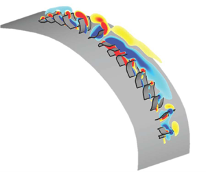
Metachronal rowing is commonly found among small swimming invertebrates, such as copepods, ctenophores, krill and shrimp. Animals that locomote via this mechanism feature rows of appendages that oscillate in a coordinated wave. This metachronal wave is induced by a phase lag between adjacent appendages, and it propagates through the row as the appendages oscillate. The beat cycle of each individual appendage consists of a power stroke and a recovery stroke. The power stroke produces thrust, while the recovery stroke generates a certain amount of drag (Sleigh Reference Sleigh1976). During the power stroke, the appendage remains fairly straight and sweeps in the direction opposite to the body's motion; during the recovery stroke, it bends and returns to its original position. Figure 1 shows the power stroke and recovery stroke of a row of appendages (e.g. cilia) engaged in metachronal motion.

Figure 1. Diagram showing (a) the beat cycle of a single rowing appendage (e.g. a cilium) and (b) a row of appendages oscillating together in a coordinated metachronal wave. The power stroke is shown in red, and the recovery stroke is shown in blue. In this figure, the direction of the metachronal wave is opposite to the direction of the appendages' power stroke, which indicates that the wave is antiplectic (Knight-Jones Reference Knight-Jones1954).
1.1. Hydrodynamic performance
Previous studies have identified several factors that influence the performance of metachronal-rowing-based propulsion. Such factors include (but are not limited to) beat frequency, number of appendages and phase lag between adjacent appendages (Murphy et al. Reference Murphy, Webster, Kawaguchi, King and Yen2011; Byron et al. Reference Byron2021). By altering the flow in the vicinity of each appendage, these factors can modify fluid displacement and the associated hydrodynamic performance. Barlow & Sleigh (Reference Barlow and Sleigh1993) studied the effects of beat frequency of a ctenophore's rowing appendages (ctenes) on the water propulsion speeds. They observed that, as beat frequency increases, the propagation velocity of the metachronal wave increases, and the phase lag between adjacent ctenes (expressed as a percentage of the total cycle time) also increases. As a consequence, the water flow speed increases proportional to the appendage tip speed, and the power output of the metachronal wave increases exponentially. Another factor that can modify flow transport of metachronal rowing is the number of appendages. Gueron & Levit-Gurevich (Reference Gueron and Levit-Gurevich1999) modelled ciliary propulsion using various numbers of beating appendages. They showed that the efficiency of metachronal rowing improves as the number of appendages increases. While this analysis is only valid for very low Reynolds numbers ( $Re \ll 1$, where $Re \equiv UL/\nu $ with U as a representative velocity scale, L a representative length scale and $\nu $ the fluid kinematic viscosity), it suggests that interactions between rowing appendages are likely to enhance the hydrodynamic performance of metachronal rowing. Colin et al. (Reference Colin, Costello, Sutherland, Gemmell, Dabiri and Du Clos2020) studied several species that swim at much higher Re, including ctenophores, annelid worms and arthropods. They found that these metachronal swimmers generate thrust by producing negative pressure along the leeward side of their appendages. This phenomenon, called ‘suction thrust’, is a result of the bending kinematics of the rowing appendages.
Another key factor that influences the hydrodynamic performance of metachronal rowing is the phase lag between appendages. To examine the effects of phase lag, Alben et al. (Reference Alben, Spears, Garth, Murphy and Yen2010) compared a krill's metachronal kinematics with synchronous kinematics, in which the phase lag is zero. They observed that metachronal rowing results in a higher average body speed. Ford & Santhanakrishnan (Reference Ford and Santhanakrishnan2021b) reached a similar conclusion through particle image velocimetry measurements of a robotic krill. They also noticed that, when a phase lag is introduced, the robotic krill's body velocity decreases as appendages move toward each other and increases as they move apart. This finding further indicates that the performance benefits of metachronal rowing are due to hydrodynamic interactions between appendages.
1.2. Vortex interactions
For all forms of drag-based paddling at sufficiently high Reynolds numbers, an appendage generates tip vortices over one beat cycle that contribute to thrust generation (Kim & Gharib Reference Kim and Gharib2011). As appendages beat in a metachronal wave, these tip vortices interact in various ways that influence hydrodynamic performance. In general, vortex interactions can be characterized as either constructive or destructive (Gopalkrishnan et al. Reference Gopalkrishnan, Triantafyllou, Triantafyllou and Barrett1994). Vortices are strengthened by constructive interactions, and they are weakened or destroyed by destructive interactions. Only a few previous studies have examined the tip vortex interactions that occur during metachronal rowing. Ford & Santhanakrishnan (Reference Ford and Santhanakrishnan2021a) used a simplified two-link model to study krill propulsion (Re ≈ 300). By decreasing the distance between adjacent appendages, they found that counterrotating tip vortices merge to form a horizontally oriented wake, thereby improving the hydrodynamic performance of metachronal rowing. In another study, Garayev & Murphy (Reference Garayev and Murphy2021) examined the tip vortex interactions among a mantis shrimp's pleopods. They identified a mechanism in which the vortex formed by the anteriormost pleopod pair is intercepted and strengthened by the posteriormost pleopod pair. This mechanism improves the mantis shrimp's swimming speed and efficiency, but the authors note that it is likely effective only at relatively high Reynolds numbers (Re ≈ 5000). This is because at low Reynolds numbers (Re < 100), tip vortices do not readily shed into the wake. Granzier-Nakajima, Guy & Zhang-Molina (Reference Granzier-Nakajima, Guy and Zhang-Molina2020) showed that, at low Re (≈1), tip vortices remain attached to an appendage throughout its beat cycle. They also demonstrated that as Re increases and inertial forces increasingly dominate (Re ≈ 100), tip vortices tend to detach from the beating appendages. To examine tip vortex interactions at intermediate Reynolds numbers, Dauptain, Favier & Bottaro (Reference Dauptain, Favier and Bottaro2008) ran numerical simulations of ctenophore swimming (Re ≈ 50). By artificially increasing the distance between adjacent appendages, they showed that as the distance increases, the thrust-to-power ratio of the appendages decreases. This observation supports the hypothesis that tip vortex interactions enhance hydrodynamic performance. However, the exact propulsion enhancement mechanism of such attached tip vortex interactions remains unknown.
1.3. Variation of size and shape
In nature, metachronal-rowing-based propulsion can be found in a wide variety of species, ranging in size from paramecia (body-scale Re ≈ 0.2) (Zhang et al. Reference Zhang, Jana, Giarra, Vlachos and Jung2015) to lobsters (body-scale Re ≈ 7500) (Lim & DeMont Reference Lim and DeMont2009). Among these species, ctenophores (body-scale Re ≈ 100–6000) are the largest animals that locomote using cilia, which beat with an appendage-scale Re of 10–300 (Matsumoto Reference Matsumoto1991). Unlike larger metachronal appendages such as those found in krill (Murphy et al. Reference Murphy, Webster, Kawaguchi, King and Yen2011) and lobsters (Lim & DeMont Reference Lim and DeMont2009), ctenophore cilia are fully flexible and therefore exhibit different bending kinematics. Ctenophore therefore present a unique opportunity to study the vortex dynamics of ciliary propulsion, a common biological propulsion system used across the low-to-intermediate Reynolds number regime. As shown in figure 2, ctenophores have eight rows containing multiple appendages called ctenes, and each ctene consists of thousands of long (mm-scale) cilia fused together (Afzelius Reference Afzelius1961). Several previous studies have explored the relationship between Re and ctenophore hydrodynamic performance. Barlow, Sleigh & White (Reference Barlow, Sleigh and White1993) increased Re for a swimming ctenophore by adjusting its ctene beating frequency. They found that, as Re increases, high-speed flow detaches from the ctene tip and is shed into the flow stream. In a separate study, Herrera-Amaya et al. (Reference Herrera-Amaya, Seber, Murphy, Patry, Knowles, Bubel, Maas and Byron2021) examined how varying Re affects the spatio-temporal asymmetry of ctene kinematics. Their results showed that increasing Re is associated with a quicker power stroke and slower recovery stroke. In addition, the spatial asymmetry of ctene beating is reduced as Re increases. However, for very low Re ( $Re \ll 1$), symmetry must be broken in order to produce net flow. Takagi (Reference Takagi2015) demonstrated that in time-reversible flow conditions ( $Re \ll 1$), it is possible to generate thrust using a spatially symmetric stroke, as long as a phase lag is introduced between adjacent appendages. These findings indicate that varying Re, together with hydrodynamic interactions between appendages, strongly influence ctene kinematics and hydrodynamic performance. However, it is unclear how Re affects the inter-ctene flow interactions that occur during ctenophore swimming.

Figure 2. Comparison between (a) the real ctenophore body and (b) the ctene row reconstruction. The ctenophore body is lined by eight ctene rows. Each row consists of sixteen ctenes situated along a curved substrate, and each ctene contains thousands of individual cilia. The reconstructed model ctene row consists of sixteen rectangular ctene meshes situated along a curved rectangular substrate mesh. The substrate mesh is coloured grey, and the sixteen ctenes are coloured red and are labelled alphabetically.
Apart from their beating kinematics, ctenophores are also noteworthy for their diverse body morphologies. Depending on the species, ctenophores may possess lobate, oblong, roughly spherical or even ribbon-like bodies (Tamm Reference Tamm2014; Gibbons et al. Reference Gibbons, Haddock, Matsumoto and Foster2021). Despite this natural diversity of body shapes, previous studies on metachronal propulsion (as well as the large body of literature on ciliary flow) have largely assumed the substrate geometry is completely flat (Dauptain et al. Reference Dauptain, Favier and Bottaro2008; Elgeti & Gompper Reference Elgeti and Gompper2013; Granzier-Nakajima et al. Reference Granzier-Nakajima, Guy and Zhang-Molina2020; Ford & Santhanakrishnan Reference Ford and Santhanakrishnan2021a). It is therefore unknown how substrate curvature impacts the hydrodynamic performance of metachronal rowing and the inter-ctene flow interactions.
To address the aforementioned gaps in knowledge, the present study employs an in-house immersed-boundary-method-based computational fluid dynamics (CFD) solver to simulate metachronal rowing. We first reconstructed the beating kinematics of ctenophore ctenes in a row (16 ctenes) based on high-speed video of a forward-swimming ctenophore. In addition to the original reconstructed geometry, we created a sparse model (8 ctenes) by removing every other ctene along the row. We then conducted a comprehensive parametric study to investigate the flow interactions of ctenophore appendages and the effects of substrate geometry on the unsteady hydrodynamics of metachronal rowing. Simulation results were used to calculate force generation and hydrodynamic power consumption for each ctene, as well as vorticity and wake structures for the entire row. Using these results, we aim to answer three questions: (i) how ctene tip vortex interactions affect hydrodynamic performance, (ii) how varying Re affects tip vortex interactions and (iii) how varying substrate curvature affects ctene row hydrodynamics.
2. Methodology
2.1. Morphological model
A high-speed recording system was used to capture real beating kinematics of ctenophore ctenes. Ctenophores were placed inside a transparent filming vessel, and the vessel was illuminated using a collimated LED light source. Three high-speed cameras and 200 mm macro lenses were used to record the swimming ctenophore. Images were captured at 600 frames per second. This set-up is described in detail by Karakas, Maas & Murphy (Reference Karakas, Maas and Murphy2020), whose data are contemporary.
We collected 27 separate recordings of free-swimming ctenophores using the multicamera high-speed video set-up. These videos were then examined carefully, and one recording was selected for further study; in the selected recording, the ctenophore was swimming unidirectionally at an approximately constant speed, and the image acquisition was high quality for model reconstruction (the ctenes themselves were orthogonal to the plane of focus over the duration of the recording, with the beating direction in plane). The selected high-speed video was then imported into Autodesk Maya, where it was used to create a meshed model of a single ctene row. The model ctene row, shown in figure 2, consists of sixteen ctenes (labelled ‘a’ to ‘p’) situated along a curved rectangular substrate. In nature, each ctene contains thousands of cilia that are grouped into a paddle-like structure, whose thickness is very small compared with its length and width (Afzelius Reference Afzelius1961). Although ctenes include many individual cilia, they function as hydrodynamically solid surfaces (Goebel et al. Reference Goebel, Colin, Costello, Gemmell and Sutherland2020). Therefore, in this study, ctenes are modelled as rectangular membrane surfaces. As observed in the real ctenophore, larger ctenes are located near the middle of the row. In addition, the curvature of the model substrate matches the ctenophore's body curvature in the beating plane. Because we created the reconstruction based on a side-view video of the ctene row, we do not consider curvature in the plane normal to the beating plane. In our model, the substrate must be wide enough to capture real flow interactions between the ctenes and substrate. In order to achieve this, the ratio of substrate width to ctene width is 6 : 1. Details regarding ctene dimensions are included in Appendix A.
To reconstruct the swimming kinematics of the ctene row for one beat cycle, a side-view orientation of the model row was superimposed over the high-speed video of the swimming ctenophore. Then, the model ctenes were aligned with various frames of the video. Because the reconstruction was created using a side view of the ctene row, the bending of each model ctene does not vary along its width. Between the frames used for reconstruction, seven-term Fourier interpolation was used to interpolate the surface mesh over time, producing a high temporal frequency (960 time steps per beat cycle) input for our CFD solver. Figure 3 compares the reconstruction with images of the real ctenophore. Both the reconstruction and the real ctenophore exhibit a metachronal wave that travels through the ctene row as the beat cycle progresses. The direction of the metachronal wave is opposite to the direction of the ctenes’ power stroke (antiplectic) (Knight-Jones Reference Knight-Jones1954). In addition, the axes used in this study are defined in the second panel of figure 3. The x-axis extends in the direction opposite to the ctenophore's swimming direction, the y-axis points above the ctenophore's body and the z-axis extends out of the plane.

Figure 3. Time sequence of a metachronal wave propagating through the real ctene row (a) as well as the row reconstruction (b) over one beat cycle T. The power stroke direction, metachronal wave direction and ctenophore swimming direction are labelled. In the images showing the real ctene row, the body curvature is highlighted using a yellow dashed line.
2.2. Ctenophore swimming kinematics
The ctenophore used in this study has a body length (Lb) of 11.56 mm. The average ctene length (l) along the row is 0.62 mm, with a standard deviation of 0.02 mm. The ctene stroke amplitude (averaged over all sixteen ctenes in the row) is 100.50°, defined as the angle traced by the ctene tip during the power stroke. The definitions of these morphological parameters are shown in figure 4. In our high-speed video recording, the ctenophore has an approximately constant forward body velocity (Ub) of 7.35 mm s−1. The ctenes have a beating frequency ( f) of 13.04 Hz over the selected beat cycle. The ctenes beat sequentially in metachronal motion, with a constant phase lag. The phase lag (PL) is defined as the average time delay between the beat cycles of adjacent ctenes and is expressed as a percentage of the overall cycle time. The value of PL is 11.20 % in our recording. More details related to the calculation of stroke amplitude and phase lag are included in Appendix B. The tip trajectories of the reconstructed row of ctenes are shown in figure 5. From the figure, we can clearly tell that the ctenes are situated on a significantly curved substrate. The average body substrate curvature (κ) is 161.51 m−1, which is defined as 1/R, where R is the radius of the curved substrate. Because the substrate is not perfectly circular, we used a least-squares circle-fitting function to calculate R (Pratt Reference Pratt1987). We fit a circle along the region of the curved substrate occupied by the ctenes (shown in figure 4), and we calculated the curvature R of this circle. Along the length of the substrate, curvature varied from a minimum of 160.77 m−1 to a maximum of 162.74 m−1. As shown in figures 3 and 5, the ctenes are located primarily along the back half of the ctenophore's body. The distance of the first and last ctenes from the front edge of the curved body is labelled in figure 5. In addition, we evaluated the ctene tip velocity, computed as  ${U_{tip}} = \sqrt {u_{tip}^2 + v_{tip}^2 + w_{tip}^2} \; $ where utip, vtip and wtip are ctene tip velocity components in the x, y and z directions, respectively (wtip is assumed to be zero). Figure 6 shows the average tip velocity ${U_{tip}}$ for the ctenes. The power stroke is shaded grey and constitutes approximately half of the total beat cycle; it is defined as the elapsed time between the two local minima shown (Herrera-Amaya et al. Reference Herrera-Amaya, Seber, Murphy, Patry, Knowles, Bubel, Maas and Byron2021). Morphological and kinematic measurements of the ctenophore used in this study are summarized in table 1. These values are consistent with previous studies on similarly sized ctenophores (Herrera-Amaya et al. Reference Herrera-Amaya, Seber, Murphy, Patry, Knowles, Bubel, Maas and Byron2021). In addition, a Fourier-series-least-squares approximation (Blake Reference Blake1972) of the ctene kinematics is included in Appendix C, which can be used for replication and validation of our results. While the kinematics for this study were prescribed via a frame-by-frame reconstruction of the behavioural experiments, the approximation in Appendix C closely matches what is used here.

Figure 4. Diagram showing ctenophore body length (Lb), ctene length (l) and stroke amplitude ( $\varPhi$). The red dashed line in the right image indicates the region over which the body curvature was calculated.

Figure 5. Diagram showing the tip trajectories of the model ctenes. Each ctene is plotted at sixteen instances throughout one beat cycle. The ctene tip is represented using a red circle, and the tip trajectory is traced in red. The instances are spaced equally in time. Axes show the location of the ctenes in relation to the front edge of the curved body. The locations of the first and last ctenes are labelled.

Figure 6. Time course of the ctenes’ tip velocity. The solid red curve is the tip velocity, averaged over all sixteen ctenes after removing the phase shift. The pink shaded margins represent the standard deviation of the tip velocity. The power stroke is shaded in grey.
Table 1. Morphological and kinematic measurements of the ctenophore used in this study.
As a ctenophore swims, the flow around its body differs from the oscillatory flow produced by each individual ctene. To account for this difference, we define two Reynolds numbers. The body Reynolds number ( $R{e_b} = {U_b}{L_b}/v$) describes the flow around a ctenophore's body as it swims in a particular direction (where $\nu $, the kinematic viscosity of seawater, is around 1.05 mm2 s−1). Following the previous literature (Herrera-Amaya et al. Reference Herrera-Amaya, Seber, Murphy, Patry, Knowles, Bubel, Maas and Byron2021), the oscillatory Reynolds number ( $R{e_\omega } = 2{\rm \pi} f{l^2}/v$) is also used to describe flow around each ctene. Based on the measured data in table 1, Reb is 66.01, and Reω is 30.00. These Reynolds numbers are intermediate, which indicates that both viscous and inertial forces play a role in ctenophore propulsion.
2.3. Numerical method and simulation set-up
Because both viscous and inertial forces are important for the ctene propulsion, this study employs an immersed-boundary-method-based in-house CFD solver to numerically solve the three-dimensional viscous incompressible Navier–Stokes equations. The non-dimensional form of these equations can be written as
 \begin{equation}\frac{{\partial {u_i}}}{{\partial {x_i}}} = 0,\quad \frac{{\partial {u_i}}}{{\partial t}} + \frac{{\partial ({u_i}{u_j})}}{{\partial {x_j}}} ={-} \frac{{\partial p}}{{\partial {x_i}}} + \frac{1}{{Re}}\frac{\partial }{{\partial {x_j}}}\left( {\frac{{\partial {u_i}}}{{\partial {x_j}}}} \right),\end{equation}
where ui are the velocity components, p is the pressure and Re is the Reynolds number.
The above equations are discretized using a cell-centred collocated grid arrangement of the primitive variables (ui and p). The fractional step method is used to integrate the equations in time, and a second-order central difference scheme is used in space. An immersed-boundary-method-based approach is applied to handle the complex moving boundaries of the beating ctenes. In this method, boundary conditions are imposed on the immersed boundaries through a ghost-cell procedure. Compared with boundary-conforming methods, such as curvilinear grid (Visbal & Gaitonde Reference Visbal and Gaitonde2001, Reference Visbal and Gaitonde2002; Visbal & Rizzetta Reference Visbal and Rizzetta2002) and finite-element methods (Tezduyar Reference Tezduyar2004; Tezduyar et al. Reference Tezduyar, Sathe, Keedy and Stein2006; Löhner Reference Löhner2008), the immersed-boundary-method approach eliminates the need for complicated re-meshing algorithms. It thus significantly reduces the computational cost associated with simulating flow past complex moving boundaries. Immersed-boundary methods can be broadly divided into two categories: the continuous forcing approach (Peskin Reference Peskin1972; Goldstein, Handler & Sirovich Reference Goldstein, Handler and Sirovich1993; Taira & Colonius Reference Taira and Colonius2007) and the discrete forcing approach (Ye et al. Reference Ye, Mittal, Udaykumar and Shyy1999; Kim, Kim & Choi Reference Kim, Kim and Choi2001; Dong et al. Reference Dong, Mittal, Bozkurttas, Lauder and Madden2010). The present study employs a multi-dimensional ‘ghost-cell’ methodology to impose the boundary conditions on the immersed boundary (Mittal et al. Reference Mittal, Dong, Bozkurttas, Najjar, Vargas and von Loebbecke2008). This method can be categorized as a discrete forcing approach, wherein forcing is directly incorporated into the discretized Navier–Stokes equations (Mittal & Iaccarino Reference Mittal and Iaccarino2005). The movement of the immersed boundaries (ctenes) were prescribed according to the image-based reconstruction as described in § 2.1. This immersed-boundary method has successfully been used to simulate insect flight (Li, Dong & Zhao Reference Li, Dong and Zhao2018, Reference Li, Dong and Zhao2020; Li Reference Li2021; Lionetti, Hedrick & Li Reference Lionetti, Hedrick and Li2022) and bio-inspired propulsion (Li & Dong Reference Li and Dong2016; Li et al. Reference Li, Wang, Liu, Deng and Dong2019; Li, Dong & Cheng Reference Li, Dong and Cheng2020; Lei, Crimaldi & Li Reference Lei, Crimaldi and Li2021). Validations of the current in-house CFD solver can be found in our previous studies (Li, Dong & Liu Reference Li, Dong and Liu2015; Li & Dong Reference Li and Dong2017; Li et al. Reference Li, Jiang, Dong and Zhao2017; Lei & Li Reference Lei and Li2020). In addition, as seen in Appendix D, our current CFD results are consistent with previous experimental measurements reported by Barlow & Sleigh (Reference Barlow and Sleigh1993) and Colin et al. (Reference Colin, Costello, Sutherland, Gemmell, Dabiri and Du Clos2020), which further proves the validity of the current CFD solver.
Figure 7 shows a schematic of the computational grid and boundary conditions employed in this study. The meshed ctene row was situated at the bottom of a non-uniform Cartesian computational grid that contained two defined layers. The ctene row was located within a very high-density region, and this region was surrounded by a secondary dense layer. Beyond this secondary layer, the grid was stretched rapidly. A constant velocity inflow was specified at the front of the fluid domain, representing the constant swimming speed, and an outflow boundary condition was applied at the back of the domain. All remaining boundaries were assigned a zero-gradient boundary condition. To achieve a periodic stage, simulations were run for four ctene beat cycles; the kinematics of each beat cycle were identical. By inspecting the time history of the force coefficients, we found that in all simulation cases, the flow reaches a nearly periodic state after two beat cycles. Results presented in this paper are based on the fourth cycle.

Figure 7. Schematic of the computational grid and boundary conditions used in this study. The computational grid is of size 352 × 210 × 114. The model ctene row consists of a curved rectangular substrate and sixteen rectangular ctene meshes, and it contains approximately 7000 triangle elements.
We performed a parametric study to evaluate how ctene tip vortex interactions, Reynolds number and substrate curvature affect the hydrodynamic performance of a forward-swimming ctenophore. To study the effects of tip vortex interactions, we created a sparse ctene row model that features a greater distance between appendages. This increased distance enabled the observation of ctene hydrodynamics with minimum effects of vortex interactions. The sparse row was a modification of the original reconstruction, formed by removing every other ctene along the row while preserving the original kinematics. The original row and sparse row are compared in figure 8. To evaluate the hydrodynamics of ctene rows across different flow regimes, we simulated kinematics at different Reynolds numbers (7.5 < Reω < 120) by adjusting the kinematic viscosity in our simulation set-up. To examine the effects of substrate curvature, we progressively flattened the model substrate used in this study. The details of how we flattened the curved substrate are documented in Appendix E. While keeping other parameters the same, we ran simulations using four different substrate curvatures, including the original curvature, medium curvature, low curvature and flat. These substrate geometries are compared in figure 9, and their calculated curvatures are listed in table 2. Table 3 provides a concise summary of all the parameters involved and their range of variation.

Figure 8. Perspective view (a) and side view (b) of the original and sparse ctene rows.

Figure 9. Perspective view (a) and side view (b) of the different substrate geometries. (Original spacing is shown; curvature variation was also explored with the sparse row.)
Table 2. Calculated curvature for each substrate geometry.

Table 3. Summary of different cases involved in the parametric study.

To evaluate hydrodynamic performance, we obtained the surface pressure and shear stress distributions along the ctene surfaces by solving the Navier–Stokes equations. Then, we calculated the instantaneous aerodynamic forces by integrating the pressure and shear stress along the surface of the model ctenes. The instantaneous lift FL and thrust FT were determined by projecting the integrated force onto the vertical and horizontal directions, respectively. In this paper, forces are presented as non-dimensional coefficients, which are computed as  ${C_L} = {F_L}/0.5\rho U_{tip}^2S$ and ${C_T} = {F_T}/0.5\rho U_{tip}^2S$. Here, ${C_L}$ and ${C_T}$ represent the lift and thrust coefficients, ${U_{tip}}$ is the ctene tip velocity, averaged over all ctenes in the row and S denotes the area of the ctene surface, averaged over all ctenes in the row. The total force coefficient is then calculated by ${C_F} = \sqrt {C_L^2 + C_T^2} $. The instantaneous hydrodynamic power ( ${P_{hydro}} = \oint { - (\bar{\bar{\boldsymbol{\mathsf{\sigma}}}}\boldsymbol{\cdot}\boldsymbol{n})\boldsymbol{\cdot}\boldsymbol{V}\,\textrm{d}s}$) is defined as the rate of output work done by the ctene model, where $\mathrm{\oint }$ denotes the integration along the model surface, $\bar{\bar{\boldsymbol{\mathsf{\sigma}}}}$ and $\boldsymbol{V}$ represent the stress tensor and the velocity vector of the fluid adjacent to the model surface and $\boldsymbol{n}$ is the normal vector of each triangular element on the model surface. Its non-dimensional coefficient ( ${C_{PW}}$) is calculated as ${C_{PW}} = {P_{hydro}}/0.5\rho U_{tip}^3S$. The immersed-boundary method employed in this study (Mittal et al. Reference Mittal, Dong, Bozkurttas, Najjar, Vargas and von Loebbecke2008) is well suited for calculating the aero/hydrodynamic performance of membranous surfaces such as ctenophore ctenes. This method has previously been used to simulate flapping membranous wings (Li et al. Reference Li, Dong and Zhao2018; Li Reference Li2021; Lionetti et al. Reference Lionetti, Hedrick and Li2022).
3. Results and discussion
In this section, the hydrodynamic performance of a ctene row is evaluated in conditions similar to a typical forward-swimming ctenophore. Ctene thrust generation and tip vortex formation are discussed in detail. To determine the effects of tip vortex interactions, the original reconstruction is compared with a modified sparse ctene row. In addition, ctene performance and vortex structures are presented for different values of Re (7.5 < Reω < 120). Finally, effects of substrate curvature are also discussed.
3.1. Ctene hydrodynamics
The in-house CFD solver was used to evaluate the hydrodynamic performance of the ctene row reconstruction shown in figure 2, as outlined in § 2.3. The time-varying instantaneous thrust produced by each of the sixteen ctenes is displayed in figure 10. Figure 10(a) shows the thrust generated by ctenes ‘a’–‘d’, which are located at the front of the row (see figure 5). This force history provides insight into how ctene bending kinematics influence thrust generation throughout the beat cycle. During the power stroke, thrust peaks as the ctene straightens and sweeps forward. During the recovery stroke, some drag is generated as the ctene deforms and returns to its original position. Due to the spatio-temporal asymmetry of the beat cycle (Herrera-Amaya et al. Reference Herrera-Amaya, Seber, Murphy, Patry, Knowles, Bubel, Maas and Byron2021), the amount of thrust produced by a ctene's power stroke is greater than the drag produced by its recovery stroke. Ctenes ‘a’–‘d’ generate a relatively small amount of thrust due to their size, as well as their orientation with respect to the ctenophore's swimming direction. As a result of the ctenophore's body curvature, the orientation of ctenes near the front of the row differs from ctenes further along the row. The effects of ctene orientation on thrust production will be further explored in § 3.4. As shown in figure 10(b,c), ctenes near the middle of the row (‘e’–‘l’) generate significantly more thrust during their power stroke, as well as more drag during their recovery stroke. Smaller ctenes at the end of the row (‘m’–‘p’, shown in figure 10d) also generate only a small amount of thrust with a similar magnitude to the first four ctenes ‘a’–‘d’. Figure 10(e) shows the thrust produced by all sixteen ctenes in the row. This plot demonstrates that due to the phase lag between appendages, a ctene's thrust starts to peak just as an adjacent ctene's thrust begins to decrease. Therefore, throughout the beat cycle, at least one of the ctenes contributes to thrust production, and all sixteen ctenes generate a steady (positive) average thrust (the thick black line in figure 10e). This effect may be likened to the functioning of a sixteen-cylinder engine, in which torque is maintained by the sequential firing of the sixteen pistons.

Figure 10. The time-dependent thrust coefficient for the sixteen ctenes throughout one beat cycle. Results are shown for ctenes (a) ‘a’–‘d’, (b) ‘e’–‘h’, (c) ‘i’–‘l’, (d) ‘m’–‘p’ and (e) all ctenes ‘a’–‘p’. The thick black line in the last panel (e) indicates the averaged thrust over all sixteen ctenes (calculated by summing the thrust produced by all sixteen ctenes, then dividing by the number of ctenes).
Figure 11 shows a schematic of the vorticity generated by a section of the ctene row at a selected time instant (t/T = 1.00). In this figure, ctene ‘f’ is in the middle of its power stroke and generates a tip vortex (v). Due to the phase lag of metachronal rowing, upstream from this vortex, ctene ‘e’ generates a smaller vortex (vu); downstream, recovering ctenes ‘g’–‘i’ produce a shear layer (vd). These vortices travel through the ctene row together as different ctenes perform their power and recovery strokes. In general, as a ctene enters its power stroke, a positive (red) vortex forms at its tip. This positive vortex contributes to the ctene's thrust generation (Kim & Gharib Reference Kim and Gharib2011). Downstream from the positive tip vortex, a negative (blue) shear layer is created as adjacent ctenes perform their recovery stroke. To illustrate the life cycle of the shear layer (vd), figure 12 identifies two locations along the row where a negative shear layer can be observed. These regions of negative vorticity are labelled vd ,1 and vd ,2. At t/T = 0.25, vd ,1 is located near the oral end of the row, and vd ,2 is located at the aboral end. As the beat cycle progresses, vd ,1 and vd ,2 travel through the row, following the propagating metachronal wave as different ctenes perform their recovery strokes. vd ,2 grows stronger as it nears the middle of the row, while vd ,1 weakens and disappears as it nears the oral end. At t/T = 1.00, vd ,2 is located approximately where vd ,1 was located at the start of the beat cycle (further illustrating the periodic nature of metachrony). In this fashion, positive tip vortices and negative shear layers travel through the row along with the metachronal wave. As these tip vortices travel through the ctene row, they undergo complex interactions with corotating and counterrotating neighbouring vortices. In the next section, we determine whether these interactions are constructive or destructive, and we examine how they affect ctene hydrodynamic performance.

Figure 11. Schematic of the vorticity produced by a portion of the ctene row at t/T = 1.00. As ctene ‘f’ performs its power stroke, it generates a tip vortex, labelled v. Upstream and downstream vortices are labelled vu and vd, respectively. The swimming direction of the ctenophore is also labelled; this is also the direction of propagation of the metachronal wave. These results were obtained using the observed natural oscillatory Reynolds number (Reω = 30).

Figure 12. Time sequence of vorticity in the ctene midplane throughout one beat cycle (see supplementary movie available at https://doi.org/10.1017/jfm.2023.739). Negative shear layers are labelled vd ,1 and vd ,2, and the sixteen ctenes are labelled alphabetically. The oral and aboral ends of the ctenophore are also labelled. The power stroke direction, metachronal wave direction and swimming direction are shown. These results were obtained using the observed natural oscillatory Reynolds number (Reω = 30).
3.2. Vortex interaction mechanism
Previous studies have suggested that vortex interactions between adjacent metachronal appendages may improve hydrodynamic performance (Ford & Santhanakrishnan Reference Ford and Santhanakrishnan2021a,Reference Ford and Santhanakrishnanb). To determine the mechanism of these interactions, we created a sparse simulation case that features a greater distance between adjacent appendages. This increased distance enabled the observation of ctene hydrodynamics without the effects of vortex interactions. The sparse case was a modification of the original reconstruction and was formed by removing every other ctene along the row. As a result, the sparse case approximately doubles the spacing and phase lag between adjacent appendages. In total, eight ctenes (‘b’, ‘d’, ‘f’, ‘h’, ‘j’, ‘l’, ‘n’ and ‘p’) were removed, and original kinematics were preserved for the remaining eight ctenes (‘a’, ‘c’, ‘e’, ‘g’, ‘i’, ‘k’, ‘m’ and ‘o’). The vorticity produced by this sparse case is shown in figure 13. As previously observed, a positive tip vortex is formed as ctenes perform their power stroke. However, due to the increased distance between appendages, recovering ctenes generate distinct negative vortices rather than an attached shear layer.

Figure 13. Time sequence of vorticity at the ctene mid-plane generated by the sparse case throughout one beat cycle (see supplemental movie). These results were obtained using the observed natural oscillatory Reynolds number (Reω = 30).
Figure 14 shows the instantaneous thrust produced by ctenes ‘g’, ‘i’ and ‘k’. Results are included for the original case and the sparse case. Both cases show that the beat cycle is divided into a thrust-producing power stroke and a drag-producing recovery stroke. However, in the sparse case, ctenes generate slightly more thrust during the power stroke and significantly more drag during the recovery stroke. To explain why this occurs, figure 15 compares the two cases (original vs. sparse) using several snapshots of the vorticity field around ctene ‘i’. For both cases, we observe two primary vortices that form during the beating cycle. A positive tip vortex forms during the power stroke (shown for ctene ‘i’ at t/T = 0.40, 0.46 and 0.52). Approximately halfway through the power stroke (t/T = 0.46), an additional negative vortex starts to form along the length of the ctene closer to the ctenophore's body. As the ctene transitions from the power stroke to the recovery stroke, the positive tip vortex disappears, and the negative vortex moves along the ctene to become the tip vortex. During the recovery stroke for the original ctene row, the tip vortex attached to ctene ‘i’ combines with adjacent tip vortices to form a negative shear layer (shown at t/T = 0.84, 0.90 and 0.96). For the sparse case, a shear layer does not form during the recovery stroke due to the increased distance between ctenes. Between the end of the recovery stroke and the start of the power stroke, the ctene undergoes a ‘rest period’ where it is relatively stationary and no obvious tip vortex is present. By comparing the tip vortices shown in figure 15, we observe that the positive power stroke tip vortex attached to ctene ‘i’ is somewhat smaller in the original case than in the sparse case, which explains why the original case generates slightly less thrust during the power stroke (see figure 14). A similar effect can be observed during the recovery stroke. The section of the recovery shear layer generated by ctene ‘i’ in the original case is much smaller than the coherent negative vortex generated by ctene ‘i’ in the sparse case.

Figure 14. Instantaneous thrust generation by ctenes ‘g’, ‘i’ and ‘k’. Results are shown for the original case and the sparse case.

Figure 15. Comparison between the original case and the sparse case. Vorticity and velocity vectors are shown at various instances during the power stroke and recovery stroke of ctene ‘i’.
Figure 16 more distinctly highlights the difference in tip vortex strength between the original and sparse cases. As tip vortex strength is closely linked to force production (Kim & Gharib Reference Kim and Gharib2011), figure 16(a) shows the instantaneous total force produced by ctene ‘i’. Throughout the beating cycle, the sparse case produces more force than the original case due to greater tip vortex circulation, as shown in figure 16(b). To calculate the circulation, we first identified the tip vortices using the  ${\lambda _2}$ criterion described by Jeong & Hussain (Reference Jeong and Hussain1995). Compared with other vortex identification methods (e.g. choosing a threshold value of vorticity), the ${\lambda _2}$ criterion is better suited for identifying vortex cores within shear flows, such as the shear layer formed by ctenes during their recovery stroke. Here, ${\lambda _2}$ is defined as the second largest eigenvalue of the tensor ${\boldsymbol{\mathsf{S}}^2} + {\boldsymbol{\mathsf{\Omega}}}^2$, where ${\boldsymbol{\mathsf{S}}}$ and ${\boldsymbol{\mathsf{\Omega}}}$ are respectively the symmetric and antisymmetric parts of the velocity gradient $\boldsymbol{\nabla }\boldsymbol{\mathsf{V}}$. Negative values of ${\lambda _2}$ denote the presence of a vortex. We calculated the circulation $\varGamma$ using $\varGamma = \int_A {\boldsymbol{\omega }\boldsymbol{\cdot }\boldsymbol{n}\,\textrm{d}A}$, where $\boldsymbol{\omega }$ is the vorticity, $\boldsymbol{n}$ is the vector normal to the surface A and A is the area enclosed by a selected contour of ${\lambda _2}$. In this study, we calculated circulation based on ${\lambda _2} ={-} 23$. We note that this threshold, while somewhat arbitrary, was chosen because it clearly distinguishes the power and recovery stroke tip vortices across the beat cycle; a lower magnitude threshold distinguishes the shear layer during the recovery stroke but does not distinguish individual vortices. Using this method, we were able to compare tip vortex circulation between the original and sparse cases. Figure 16(b) shows the circulation of the positive and negative vortices attached to ctene ‘i’ throughout its beat cycle. As described in the previous paragraph, the negative vortex that will become the recovery stroke tip vortex begins to form during the power stroke; this explains the overlap between positive and negative circulation shown in figure 16(b). This plot demonstrates that vortex circulation is always weaker in the original ctene row between t/T = 0.35 and 0.92 (comprising 57 % of the total beating cycle). It is worth noting that approximately 82 % of total force production occurs during this period, which demonstrates the importance of vortex-weakening mechanism on the overall force generation. The difference in tip vortex strength can also be observed in figure 16(c,d), which show the vorticity around ctene ‘i’ for the original and sparse cases, respectively. In these images, positive and negative vortices are labelled with ‘+ $\varGamma$’ and ‘− $\varGamma$’, and contours are shown for ${\lambda _2} ={-} 23$. At both time instances shown, the tip vortex is visibly smaller in the original ctene row. These results further demonstrate that tip vortices are weaker in the original row, resulting in reduced force production.

Figure 16. (a) The instantaneous total force produced by ctene ‘i’. (b) The normalized circulation of the tip vortex attached to ctene ‘i’, calculated using  ${\lambda _2} ={-} 23$. The vortex-weakening period is shaded in grey.(c,d) Show the vorticity around ctene ‘i’ for the original and sparse cases, respectively. The tip vortex is shown during the power stroke (t/T = 0.52) and the recovery stroke (t/T = 0.90). Positive and negative vortices are labelled with ‘+ $\varGamma$’ and ‘− $\varGamma$’, and contours are shown for ${\lambda _2} ={-} 23$.
Because tip vortices are consistently weaker in the original case, we propose that ctenophores employ a vortex-weakening mechanism to enhance their hydrodynamic performance. Through this mechanism, ctene tip vortices (both positive and negative) are weakened by destructive interactions with neighbouring vortices. In metachronal rowing, the distance between ctene tips increases during the power stroke, and ctene tips are brought closer together during the recovery stroke. As a result, destructive tip vortex interactions are minimized during the thrust-producing power stroke and maximized during the drag-producing recovery stroke. This has the overall effect of increasing the average thrust produced by the ctenes, as shown in figure 17.

Figure 17. Cycle-averaged (a) thrust generation, (b) lift generation, (c) power consumption and(d) thrust-to-power ratio for each ctene along the row. Results are shown for the original case and the sparse case. In each plot, the data were fitted using a six-term polynomial trendline. The direction of thrust and lift relative to the ctene row is shown in the inset of (a).
In figure 17, the cycle-averaged force generation (both lift and thrust), power consumption and thrust-to-power ratio (CT/CPW) for each ctene are compared between the original case and the sparse case. As shown in figure 17(a), ctenes in the original case generate more thrust, which can be attributed to the proposed vortex-weakening mechanism. This mechanism significantly reduces drag generation during the recovery stroke, which outweighs the slight decrease in thrust during the power stroke. As a result, overall thrust generation is improved (as shown via higher cycle-averaged CT). Figure 17(a) also shows that the larger ctenes near the middle of the row produce the most cycle-averaged thrust and show the largest difference in CT between the original and sparse cases.
Figure 17(b) presents the force component generated in the vertical (y) direction (lift coefficient, CL), averaged over the beat cycle. Both original and sparse cases follow a similar trend across ctenes, with similar magnitudes of lift generated for both cases. Figure 17(c) displays the average power consumed by each ctene. This plot shows that ctenes in the original case consume less power, which is another benefit of the vortex-weakening mechanism. This mechanism reduces the magnitude of instantaneous thrust production throughout the beat cycle, and as a result, ctenes consume less power. Figure 17(d) shows that the average ctene thrust-to-power ratio is higher for ctenes in the original case than ctenes in the sparse case. In both cases, the first few ctenes in the row have the lowest thrust-to-power ratio, and the last few ctenes have the greatest thrust-to-power ratio. Table 4 reports the averaged thrust generation, power consumption and thrust-to-power ratio for the entire ctene row. To make a fair comparison, these values were calculated by averaging the performance of the eight ctenes within the row (‘a’, ‘c’, ‘e’, ‘g’, ‘i’, ‘k’, ‘m’ and ‘o’) simulated in both the original and sparse cases. Compared with the original row, the sparse row generates 38.32 % less thrust, consumes 28.12 % more power and has a 55.00 % lower thrust-to-power ratio.
Table 4. Average ctene row performance for the original case and the sparse case (calculated by averaging over all ctenes in the row). For a fair comparison, only eight ctenes of the original case (‘a’, ‘c’, ‘e’, ‘g’, ‘i’, ‘k’, ‘m’ and ‘o’) are counted for the calculation.

These results indicate that the newly proposed vortex-weakening mechanism significantly improves the hydrodynamic performance of metachronal rowing. This mechanism also provides some insight into the evolution of metachronal rowing in ctenophores and other species. In a row of beating appendages, there is evolutionary pressure to increase the distance between appendages, so that thrust-enhancing tip vortices can form during the power stroke. However, there is also pressure to decrease the distance between appendages, so that drag-producing tip vortices formed during the recovery stroke can be weakened by moving appendage tips closer together. It is therefore likely that there exists an optimal combination of appendage spacing and spatio-temporal kinematics that maximizes the performance-enhancing effects of the vortex-weakening mechanism. In ctenophores, the flexibility of the appendage allows for closer spacing during the recovery stroke vs. the power stroke; the material properties and bending dynamics of ctenes may therefore have been influenced over evolutionary time by this fluid mechanical constraint on performance. Furthermore, the optimal spacing is likely to be Reynolds number dependent, as explored in the next section.
Several previous studies have examined how appendage spacing and kinematics affect hydrodynamic performance, but have not examined the underlying flow mechanisms in detail. Dauptain et al. (Reference Dauptain, Favier and Bottaro2008) found that ctenophore swimming is most efficient when the ratio of appendage spacing to appendage length is close to 0.5. This optimal spacing is likely a consequence of the vortex-weakening mechanism. As described in the previous paragraph, the distance between appendages must be large enough to allow the formation of strong tip vortices during the power stroke, but small enough to weaken tip vortices formed during the recovery stroke. Other studies have shown that metachronal rowing results in a greater average body speed than synchronous rowing, in which the phase lag is zero (Alben et al. Reference Alben, Spears, Garth, Murphy and Yen2010; Ford & Santhanakrishnan Reference Ford and Santhanakrishnan2021b). Our results indicate that a primary benefit of the phase lag, in combination with the time-varying shape of the beating ctene, is to increase the distance between ctene tips during the power stroke and reduce the distance between ctene tips during the recovery stroke. As a result, destructive tip vortex interactions are minimized during the thrust-producing power stroke and maximized during the drag-producing recovery stroke. These findings suggest that the vortex-weakening mechanism is a combined effect of multiple morphological (e.g. appendage spacing) and kinematic (e.g. phase lag and bending) parameters involved in metachronal rowing.
The identification of the vortex-weakening mechanism enhances our understanding of the hydrodynamic principles underlying metachronal rowing. For example, Colin et al. (Reference Colin, Costello, Sutherland, Gemmell, Dabiri and Du Clos2020) found that metachronal swimmers generate thrust by creating negative pressure fields along the leeward side of their appendages. In ctenophores, this ‘suction thrust’ is a result of the bending kinematics of the beating ctenes. Our findings suggest that ctene bending also promotes destructive tip vortex interactions between neighbouring appendages during the recovery stroke, which significantly improve the ctenophore's overall thrust production. The vortex-weakening mechanism can also be compared with appendage interaction mechanisms that occur across different flow regimes. In Stokes flow conditions ( $Re \ll 1$), recent studies have identified a ciliary ‘shielding effect’ in which the flow generated by a beating cilium is obstructed by adjacent cilia (Khaderi, Den Toonder & Onck Reference Khaderi, Den Toonder and Onck2011; Milana et al. Reference Milana, Zhang, Vetrano, Peerlinck, De Volder, Onck, Reynaerts and Gorissen2020; Zhang, den Toonder & Onck Reference Zhang, den Toonder and Onck2021, Reference Zhang, den Toonder and Onck2022). This effect is present throughout the entire beating cycle, but it is especially pronounced during the recovery stroke, leading to an overall increase in net flow. This shielding effect functions similarly to the vortex-weakening mechanism, as some performance is sacrificed during the power stroke to enable significant performance gains during the recovery stroke (see figure 14). However, cilia typically beat with a much lower Reynolds number ( $Re \ll 1$) than the ctenes observed in this study (Reω = 30). In the next section, we will explore how the vortex-weakening mechanism is affected by artificially increasing and decreasing Re.
3.3. Effects of varying the Reynolds number
In this section, we aim to examine how ctenophores’ propulsion mechanism changes as the Reynolds number varies between 7.5 and 120. Across this range of Reω, we ran simulations using both the original ctene row and the sparse row. Figure 18(a) shows the thrust produced by ctenes ‘g’, ‘i’ and ‘k’ in the original row. As Reω increases, less (non-dimensional) thrust is generated during the power stroke, and less drag is generated during the recovery stroke. In other words, the instantaneous magnitudes of the horizontal force coefficients are reduced throughout the beat cycle. Figure 18(b) displays similar results for the sparse row.

Figure 18. Instantaneous thrust generation by ctenes ‘g’, ‘i’ and ‘k’ at different Reynolds numbers (Reω = 7.5, Reω = 15, Reω = 30, Reω = 60, Reω = 120). Results are shown for (a) the original ctene row and (b) the sparse row.
To explain this trend, figure 19 shows how varying Reω affects the vortex structures produced by the ctene row. At lower Reynolds numbers, ctenes generate attached tip vortices and shear layers. However, as Reω increases, these vortices start to detach from the ctene tips. In the observed natural ctenophore swimming (Reω = 30), attached tip vortices and shear layers enhance ctene force production (Kim & Gharib Reference Kim and Gharib2011). Therefore, vortex detachment at higher Reω reduces the magnitude of force generation throughout the beat cycle, as shown in figure 18. These observations suggest that the vortex-weakening mechanism is more effective at improving thrust performance in the low-to-intermediate Reynolds number regime, in which tip vortices and shear layers remain attached to the beating ctenes.

Figure 19. The Q-isosurface vortex structures generated by the original ctene row at t/T = 1.00. Results are shown for Reω = 7.5, Reω = 15, Reω = 30, Reω = 60 and Reω = 120. See movie in the supplementary material.
Figure 20 shows how Reω affects the cycle-averaged ctene performance. For ctenes in the original row, average thrust production and power consumption decrease as Reω becomes larger. The decrease in thrust generation is caused by the detachment of tip vortices and shear layers, and the decrease in power consumption is a result of the thinner boundary layer at higher Reω. The ctene thrust-to-power ratio (CT/CPW) improves as Reω becomes larger. The sparse ctene row exhibits similar trends in power consumption and thrust-to-power ratio. However, unlike the original row, increasing Reω does not impact overall thrust production as dramatically, as shown in table 5. This difference is a result of the proposed vortex-weakening mechanism, which does not play a role in the sparse row.

Figure 20. Cycle-averaged thrust, power and thrust-to-power ratio for each ctene. Results are shown for Reω = 7.5, Reω = 15, Reω = 30, Reω = 60 and Reω = 120. The left column (a–c) includes results for the original ctene row, and the right column (d–f) includes results for the sparse row.
Table 5. Average ctene row performance for different values of Reω. Results are presented for the original ctene row and the sparse row.

In the original row, attached tip vortices interact to reduce the amount of drag produced by recovering ctenes. When tip vortices detach at higher Reω, this drag-reducing effect is lost and ctenes therefore generate less average thrust. The sparse ctene row does not benefit from tip vortex interactions very much, and as a result, its average thrust generation is significantly less sensitive to varying Reω. These trends are summarized in table 5, which shows the average ctene row performance for each case. As Reω increases, the original row produces less (non-dimensional) thrust, consumes less power, and its thrust-to-power ratio increases. The sparse row exhibits similar trends in power consumption and thrust-to-power ratio. However, for reasons described above, its thrust generation is less affected by changing Reω. Interestingly, when considering swimming ctenophores, animals (such as Beroe sp.) which beat their ctenes at higher frequencies (and correspondingly higher Reω) also have closer ctene spacing, indicating that the vortex-weakening mechanism may extend to higher Reω if the spacing between ctenes is decreased.
3.4. Effects of varying substrate curvature
To determine how body curvature affects ctene hydrodynamics, we progressively flattened the model substrate used in this study (for details, see Appendix E). We ran simulations using four different substrate curvatures, including the original curvature, medium curvature, low curvature and flat. For each substrate geometry, simulations were run using both the original ctene row and the sparse row (using the original ctene kinematics and Reynolds number). Figure 21 shows the vorticity produced by the original row along each of the different substrate curvatures. As previously observed, ctenes generate a positive vortex during their power stroke, and they generate a negative shear layer during their recovery stroke. These vortex formations are consistent across all four substrate curvatures. Figure 22 displays similar results for the sparse ctene row.

Figure 21. Vorticity generated by the original ctene row at t/T = 0.25. Results are shown for different substrate curvatures, including (a) the original curvature, (b) medium curvature, (c) low curvature and (d) flat.

Figure 22. Vorticity generated by the sparse ctene row at t/T = 0.25. Results are shown for different substrate curvatures, including (a) the original curvature, (b) medium curvature, (c) low curvature and (d) flat.
Figure 23 shows the cycle-averaged ctene performance for each substrate curvature. Figure 23(a) includes the average thrust produced by ctenes in the original row. For the first four ctenes (‘a’–‘d’), the original curvature generates less thrust than the other three curvatures. However, for the remaining twelve ctenes (‘e’–‘p’), the original curvature generates significantly more thrust. Figure 23(b) shows the average lift produced by ctenes in the original row. For the first five ctenes (‘a’–‘e’), all curvatures generate approximately the same amount of lift. However, for the other eleven ctenes (‘f’–‘p’), the original curvature produces less lift than the other curvatures. Average total force generation, shown in figure 23(c), remains relatively unchanged by substrate curvature.

Figure 23. Cycle-averaged ctene force generation (thrust, lift and overall force coefficients) for each substrate curvature. Results are shown for the original ctene row (a–c) and the sparse row (d–f).
Similar trends are observed for the sparse row, as seen in figure 23(d–f). In addition, figure 24 shows that as the substrate flattens, ctene power consumption remains unchanged (and, therefore, the thrust-to-power ratio decreases). These results are summarized in tables 6 and 7. Table 6 shows that as the substrate flattens, the ctene row overall generates less thrust and more lift, while its total force production is relatively unaffected. Table 7 shows that the ctene row consumes the same amount of power as it flattens, while its thrust-to-power ratio decreases. Since total force production is related to tip vortex strength, it is likely that that tip vortex circulation is also relatively unaffected by substrate curvature. This is demonstrated in figure 25, which shows the circulation of the tip vortex attached to ctene ‘i’. Between the original substrate curvature and the flat substrate, we do not observe any significant differences in tip vortex circulation. We also determined that for the original substrate curvature, vortex interactions weaken the tip vortex by a maximum of 42 % during the power stroke and 77 % during the recovery stroke. For the flat curvature, the tip vortex is weakened by a maximum of 39 % during the power stroke and 85 % during the recovery stroke. This suggests that the proposed vortex-weakening mechanism is active regardless of substrate curvature and is effective across a variety of body morphologies. We can therefore infer that the vortex-weakening mechanism is present in most instances of metachronal rowing in the low-to-intermediate Reynolds number regime, including ciliary flows (Elgeti & Gompper Reference Elgeti and Gompper2013; Granzier-Nakajima et al. Reference Granzier-Nakajima, Guy and Zhang-Molina2020), paramecia swimming (Zhang et al. Reference Zhang, Jana, Giarra, Vlachos and Jung2015) and ctenophore swimming among different species (Tamm Reference Tamm2014; Gibbons et al. Reference Gibbons, Haddock, Matsumoto and Foster2021).

Figure 24. Cycle-averaged ctene power consumption and thrust-to-power ratio for each substrate curvature. Results are shown for the original ctene row (a,b) and the sparse row (c,d).
Table 6. Average ctene row force generation for different substrate curvatures. Results are presented for the original ctene row and the sparse row.

Table 7. Average ctene row power consumption and thrust-to-power ratio for different substrate curvatures. Results are presented for the original ctene row and the sparse row.


Figure 25. Effects of substrate curvature on the circulation of the tip vortex attached to ctene ‘i’. Results are shown for the original substrate curvature and the flat substrate using the original ctene row and the sparse row.
As previously mentioned, total ctene force production, power consumption and tip vortex circulation are not significantly affected by substrate curvature. This indicates that the performance benefits (as measured by higher CT) of a curved substrate are not a result of vortex interactions or other unsteady flow features. We therefore hypothesize that, in our simulations, varying the substrate curvature (while preserving the original kinematics) affects ctenophore hydrodynamic performance simply by reorienting the direction of ctene motion. To illustrate the effects of ctene orientation, figure 26 depicts the thrust and lift vectors produced by ctene ‘k’ as it experiences maximum force production. Figure 26(a) shows that in the original substrate curvature, ctene ‘k’ is oriented perpendicular to the ctenophore's swimming direction. In this orientation, it generates mostly thrust and almost no lift. Figure 26(b) shows that in the flat substrate curvature, ctene ‘k’ is more parallel to the ctenophore's swimming direction. In this orientation, it produces less thrust and more lift. Based on these observations, we conclude that most of the ctenes along the original substrate are oriented so that during the peak of their power stroke, they are roughly perpendicular to the ctenophore's direction of motion. As a result, these ctenes displace fluid directly behind the ctenophore's body, which maximizes their thrust generation. In contrast, ctenes along the reconstructed flat substrate experience their maximum force production while oriented more parallel to the ctenophore's direction of motion. Therefore, ctenes along the flat substrate generate less thrust and more lift.

Figure 26. Vector diagram showing the thrust (coloured red) and lift (coloured blue) produced by each ctene at t/T = 0.15. At this particular time instant, ctene ‘k’ (shown in subplot) is experiencing maximum force production. Results are compared between (a) the original and (b) flat substrate curvatures.
The same trend is observed for most of the ctenes in the row. This is demonstrated in figure 27, which shows the average thrust and lift vectors for each ctene along the different substrate curvatures. As the substrate curvature flattens, ctenes on average generate less thrust and more lift. However, in real ctenophore forward swimming, lift does not contribute to propulsion due to radial symmetry (as illustrated in the subplot of figure 27a). Due to the symmetrical arrangement of ctene rows around the ctenophore's body, lift generated by one row is negated by the row located directly across the body. Because the original substrate curvature generates the least lift and most thrust, it provides the best hydrodynamic performance of the four curvatures tested. However, this is because we preserved the original ctene kinematics while rotating them into a flat configuration (see Appendix E). Real ctenophores have a high degree of variability in body curvature, and it is likely that the ctene kinematics are tuned to accommodate this variability; this may be accomplished by altering the position of the stroke amplitude ‘cone’ shown in figure 4 and/or the shape of the power and recovery strokes to ensure that force production is maximized in the swimming direction. Future investigations of living animals may wish to focus on how ctenes are oriented with respect to the body wall throughout the beat cycle, and how this varies with body curvature.

Figure 27. Vector diagram showing the average thrust (coloured red) and lift (coloured blue) produced by each ctene. Results are shown for different substrate curvatures, including (a) the original curvature, (b) medium curvature, (c) low curvature and (d) flat. Average ctene row force vectors are shown above each curvature. See movie in the supplementary material.
Another interesting effect of body curvature is that for the first few ctenes in the row (‘a’–‘d’), the flat substrate produces the most thrust and displays the highest thrust-to-power ratio. In fact, ctenes ‘a’ and ‘b’ along the original curvature even generate a small amount of drag, as shown in figure 23(a). For ctenes further along the row (‘e’–‘p’), this trend reverses, and the original curvature provides far superior performance. Figures 26 and 27 help illustrate why this shift occurs. In the original curvature, the first few ctenes are angled slightly toward the front of the ctenophore's body, leading to diminished thrust and, for ctenes ‘a’ and ‘b’, slight drag. Further along the row, ctenes are angled behind the ctenophore's body, which is a more optimal configuration for thrust production. This is a primary reason why, in nature, ctenes are located mainly along the back half of the ctenophore's body. However, ctenophores are capable of a wide variety of swimming manoeuvres, including near-omnidirectional swimming and turning (Herrera-Amaya & Byron Reference Herrera-Amaya and Byron2023). This could account for the presence of ctenes ‘a’ and ‘b’; although they slightly degrade the ctenophore's thrust generation, they likely contribute to performance in other modes of swimming.
4. Conclusions
In this study, we simulated ctenophore swimming kinematics using an in-house immersed-boundary-method-based CFD solver. Our simulation results show that ctenes form a thrust-producing tip vortex during their power stroke and a drag-producing shear layer during their recovery stroke. As ctenes beat metachronally, these vortices interact to enhance hydrodynamic performance. We propose that this enhancement occurs via destructive interactions between neighbouring tip vortices. Ctene tips move apart during their power stroke and move toward each other during their recovery stroke. As a result, destructive tip vortex interactions are minimized during the thrust-producing power stroke and are maximized during the drag-producing recovery stroke. To quantify the effects of this vortex-weakening mechanism, we created an artificial ‘sparse’ simulation case in which the distance between ctenes is approximately doubled. Compared with the sparse case (in which vortex interactions are greatly reduced), we found that the vortex-weakening mechanism increases overall thrust production, decreases power consumption and increases the thrust-to-power ratio. In addition, we found that the performance of the vortex-weakening mechanism is dependent on the Reynolds number. As Re increases, tip vortices detach from the beating ctenes. Because the vortex-weakening mechanism is caused by interactions between ctene tip vortices, it becomes much less effective when tip vortices detach at higher Re. However, thrust-to-power ratio increases as Re increases, indicating that metachronal propulsion may be effective at higher Re as well as the low-to-intermediate Re at which it is typically observed. Additionally, the vortex-weakening mechanism may be extended to higher Re if ctene spacing is smaller, as observed in some ctenophore species.
In nature, ctenophores can possess a wide variety of different body morphologies. To determine how body geometry affects ctenes’ performance and vortex interactions, we examined the hydrodynamics of ctenophore ctenes situated along substrates with different body curvatures. Our results show that if ctene kinematics are preserved and substrate curvature is decreased, overall thrust decreases and overall lift increases. This indicates that ctenophores most likely orient their ctenes and vary beating kinematics to maximize thrust production and minimize lift production across different curvatures/morphologies. In other words, ctene (and cilia) kinematics for a highly curved substrate are unlikely to be identical to those operating on a flatter substrate; this represents a promising direction for future study. We also demonstrated that the substrate curvature has little effect on the vortex-weakening mechanism, which indicates that this mechanism is effective across a variety of different body morphologies.
In this study, we identified a new vortex-weakening mechanism that enhances the performance of metachronal rowing. Our findings suggest that there is an optimal relationship of morphological (e.g. appendage spacing) and kinematic (e.g. phase lag) parameters that maximizes the effectiveness of this mechanism. Further examination of this relationship could yield new insights into how metachronal rowing performs across different scales and species, as well as guide the development of bio-inspired swimming robots.
Supplementary movie
Supplementary movie is available at https://doi.org/10.1017/jfm.2023.739.
Acknowledgements
We thank E. Seber (Penn State), D. Murphy, F. Karakas and D. Olsen (University of South Florida) as well as A. Maass and A. Miccoli (BIOS) for assistance with data collection. All simulations were run on the High-Performance Computing Cluster of the College of Engineering at Villanova University.
Funding
This research was supported by grants from the National Science Foundation to C.L. (NSF CBET-2120505) and to M.L.B. (NSF CBET-2120689), as well as a Grant-In-Aid (Samuel Riker Fellowship) from the Bermuda Institute of Ocean Sciences (BIOS).
Declaration of interests
The authors report no conflict of interest.
Appendix A. Ctene dimensions
The length of each ctene in the model row matches the length of the real ctene in the high-speed video used for reconstruction. The width of the model ctenes is assumed to be constant, consistent with previous computational studies on metachronal rowing (Dauptain et al. Reference Dauptain, Favier and Bottaro2008; Granzier-Nakajima et al. Reference Granzier-Nakajima, Guy and Zhang-Molina2020). Although the actual ctenophore has slightly narrower ctenes near the end of the row compared with those in the middle, we assume this variation is minimal; width variation over the time course of the beat cycle for a single ctene (not accounted for in our model) is likely to be much more significant (Goebel et al. Reference Goebel, Colin, Costello, Gemmell and Sutherland2020), of the order of 30 % greater during the power stroke vs. the recovery stroke. Therefore, our simulations likely underestimate overall force production by an amount that is greater than that resulting from a systematic difference in ctene width. Furthermore, we believe that the constant width assumption does not significantly impact our study's overall conclusions. The length and aspect ratio of the model ctenes are recorded in table 8.
Table 8. Length and aspect ratio of the model ctenes.

Appendix B. Calculation of stroke amplitude and phase lag
In this study, we define the stroke amplitude  $\varPhi$ as the angle traversed by the ctene tip during the power stroke. This definition is illustrated in figure 28(a), which shows a time sequence of a ctene's motion throughout its beating cycle. The positions of the ctene at the beginning and end of the power stroke are shown in red, and the stroke angle is measured between the ctene tips at these positions. We define the phase lag PL between two neighbouring ctenes as the time difference between their respective moments of maximum tip velocity. This definition is shown in figure 28(b), which uses the tip velocities of ctenes ‘i’ and ‘j’ as a representative example.

Figure 28. Images showing how (a) the stroke amplitude  $\varPhi$ and (b) the phase lag PL were calculated.
Appendix C. Ctene kinematics
To make our work replicable, we provide an approximate model of ctene kinematics using the Fourier-series-least-squares (FS-LS) method developed by Blake (Reference Blake1972). Since ctenes are modelled as rectangular membrane surfaces, we use the centreline in an XOY cross-sectional plane as a representation of the whole membrane. As shown in figure 29, the centreline of a certain single ctene is discretized into I pieces, where each point on the centreline is denoted by  ${s_i}$ (i = 0, 1, …, I), which measures the arclength from the ctene root. Since the reconstructed model gives the trajectory data of any arbitrary point i in one period in the form of the coordinates ${X_i}({s_i},t)$ and $Y({s_i},t)$, we can approximate these data along a time course using a Fourier series.

Figure 29. Illustration of the notation.
The truncated FS equation is given by (C1) and (C2)
 \begin{gather}{X_i}({s_i},t) = \frac{1}{2}{a_{0,x}}({s_i}) + \sum\limits_{n = 1}^N {\left[ {{a_{n,x}}({s_i})\,\textrm{cos}\left( {\frac{{2n{\rm \pi} }}{T}t} \right) + {b_{n,x}}({s_i})\,\textrm{sin}\left( {\frac{{2n{\rm \pi} }}{T}t} \right)} \right]}, \end{gather}
 \begin{gather}{Y_i}({s_i},t) = \frac{1}{2}{a_{0,y}}({s_i}) + \sum\limits_{n = 1}^N {\left[ {{a_{n,y}}({s_i})\,\textrm{cos}\left( {\frac{{2n{\rm \pi} }}{T}t} \right) + {b_{n,y}}({s_i})\,\textrm{sin}\left( {\frac{{2n{\rm \pi} }}{T}t} \right)} \right]} ,\end{gather}
where T is the beating period and N represents the number of terms in the FS. Here,  ${a_{0,x}}({s_i})$, ${a_{n,x}}({s_i})$ and ${b_{n,x}}({s_i})$ are the FS coefficients in the x direction obtained from the known trajectory, and ${a_{0,y}}({s_i})$, ${a_{n,y}}({s_i})$ and ${b_{n,y}}({s_i})$ are the coefficients in the y direction. Then, the resulting coefficients are fitted into polynomial equations using the linear least-squares method in (C3) and (C4)
 \begin{gather}{a_{n,x}}({s_i}) = \sum\limits_{m = 1}^M {{A_{mn,x}}{s^m}} ,\quad {b_{n,x}}({s_i}) = \sum\limits_{m = 1}^M {{B_{mn,x}}{s^m}} ,\end{gather}
 \begin{gather}{a_{n,y}}({s_i}) = \sum\limits_{m = 1}^M {{A_{mn,y}}{s^m}} ,\quad {b_{n,y}}({s_i}) = \sum\limits_{m = 1}^M {{B_{mn,y}}{s^m}} ,\end{gather}
where  ${A_{mn,x}}$ and ${B_{mn,x}}$ are the polynomial coefficients in the x direction, and ${A_{mn,y}}$ and ${B_{mn,y}}$ are the coefficients in the y direction. Once we solve for the polynomial coefficients, we can derive the kinematics model by substituting (C3) and (C4) into (C1) and (C2). Thus, the FS-LS model yields (C5) and (C6)
 \begin{align}{X_i}({s_i},t)
&= \frac{1}{2}\sum\limits_{m = 1}^M {{A_{m0,x}}{s^m}} +
\sum\limits_{n = 1}^N \left[\sum\limits_{m = 1}^M
{\left[ {{A_{mn,\; x}}{s^m}\,\textrm{cos}\left(
{\frac{{2n{\rm \pi} }}{T}t} \right)} \right]}\right.\nonumber\\
&\quad +\left. \sum\limits_{m =
1}^M {\left[ {{B_{mn,x}}{s^m}\,\textrm{sin}\left(
{\frac{{2n{\rm \pi} }}{T}t} \right)} \right]} \right]
, \end{align}
\begin{align}{X_i}({s_i},t)
&= \frac{1}{2}\sum\limits_{m = 1}^M {{A_{m0,x}}{s^m}} +
\sum\limits_{n = 1}^N \left[\sum\limits_{m = 1}^M
{\left[ {{A_{mn,\; x}}{s^m}\,\textrm{cos}\left(
{\frac{{2n{\rm \pi} }}{T}t} \right)} \right]}\right.\nonumber\\
&\quad +\left. \sum\limits_{m =
1}^M {\left[ {{B_{mn,x}}{s^m}\,\textrm{sin}\left(
{\frac{{2n{\rm \pi} }}{T}t} \right)} \right]} \right]
, \end{align} \begin{align}{Y_i}({s_i},t)
&= \frac{1}{2}\sum\limits_{m = 1}^M {{A_{m0,y}}{s^m}} +
\sum\limits_{n = 1}^N \left[ \sum\limits_{m = 1}^M
{\left[ {{A_{mn,y}}{s^m}\,\textrm{cos}\left( {\frac{{2n{\rm \pi}
}}{T}t} \right)} \right]}\right.\nonumber\\
&\quad +\left. \sum\limits_{m = 1}^M {\left[
{{B_{mn,y}}{s^m}\,\textrm{sin}\left( {\frac{{2n{\rm \pi} }}{T}t}
\right)} \right]} \right], \end{align}
\begin{align}{Y_i}({s_i},t)
&= \frac{1}{2}\sum\limits_{m = 1}^M {{A_{m0,y}}{s^m}} +
\sum\limits_{n = 1}^N \left[ \sum\limits_{m = 1}^M
{\left[ {{A_{mn,y}}{s^m}\,\textrm{cos}\left( {\frac{{2n{\rm \pi}
}}{T}t} \right)} \right]}\right.\nonumber\\
&\quad +\left. \sum\limits_{m = 1}^M {\left[
{{B_{mn,y}}{s^m}\,\textrm{sin}\left( {\frac{{2n{\rm \pi} }}{T}t}
\right)} \right]} \right], \end{align}where the number of FS terms is N = 3 and the number of polynomial terms is M = 3.
Tables 9–12 summarize the values of the coefficients  ${A_{mn}}$ and ${B_{mn}}$ for the x and y directions, which represent the approximate models of ctenes ‘a’–‘p’. To replicate the kinematics of the reconstructed model in our simulations, the readers can discretize their centreline model into arbitrary pieces and calculate the arclength from the root for each point. Then, input the provided coefficients into (C5) and (C6) to calculate coordinates of each point at any time instance within one beating period.
Table 9. Fourier-least-squares coefficients for ctenes ‘a’–‘d’.

Table 10. Fourier-least-squares coefficients for ctenes ‘e’−‘h’.

Table 11. Fourier-least-squares coefficients for ctenes ‘i’−‘l’.

Table 12. Fourier-least-squares coefficients for ctenes ‘m’−‘p’.

Appendix D. Validation of computational modelling
To validate the CFD solver used in the current study, we calculated the power output of each ctene using the method described by Barlow & Sleigh (Reference Barlow and Sleigh1993). In this previous study, the authors estimated a ctenophore's power output using the water jet produced by the beating ctenes. The peak power P in a water jet is defined as  $P = {\textstyle{1 \over 2}}\mathrm{\rho }{u^3}A$, where ρ is the density of seawater (1027 kg m−3), u is the peak flow speed within the jet and A is the cross-sectional area of the jet. The cross-sectional area A is approximated by extending a line from the velocity contour corresponding to the peak flow u to the contour corresponding to ~20 % u. This distance is treated as the radius of a cylindrical water jet.
Using the results from our CFD simulation, we replicated this process to estimate the peak power output of each of the sixteen model ctenes. Figure 30 compares the results from the current study with those obtained by Barlow & Sleigh (Reference Barlow and Sleigh1993). In this figure, ctene power output is plotted as a function of peak tip speed. Our results agree reasonably well with the previous study, and both studies show that power output increases exponentially with tip speed.

Figure 30. Plot showing the relationship between peak power output and peak ctene tip speed. Results from the current study are compared with results calculated by Barlow & Sleigh (Reference Barlow and Sleigh1993). The data from each study are fitted using a least-squares exponential trendline.
We also validated the solver by comparing the thrust generated by ctene ‘i’ with experimental results obtained by Colin et al. (Reference Colin, Costello, Sutherland, Gemmell, Dabiri and Du Clos2020). By considering the width of ctene ‘i’ (1.03 mm), we were able to approximate its thrust production per metre in the z-direction, yielding units of N m−1 consistent with the measurements in the previous study. Results for the thrust generated by a ctene during its power stroke are compared in figure 31. In general, both studies exhibit a similar overall trend, and thrust generation is of the same order of magnitude. However, the previous study displays a larger magnitude of thrust compared with our CFD results. The discrepancies of the thrust magnitude between our results and the previous experimental measurements could be explained by differences in ctenophore body size, swimming conditions or ctene morphology. Another potential reason for this discrepancy is that the previous study calculated thrust based on two-dimensional flow measurements, which potentially ignored certain three-dimensional flow phenomena such as the edge/tip vortices formed by a finite-aspect-ratio ctene. This could lead to an overestimation of thrust generation relative to our simulation.

Figure 31. Plot showing instantaneous thrust generated by a single ctene during its power stroke. Results from the current computational study are compared with experimental results obtained by Colin et al. (Reference Colin, Costello, Sutherland, Gemmell, Dabiri and Du Clos2020).
In addition, we found that the vortex formed during the power stroke of ctene ‘i’ is comparable to results obtained by Colin et al. Figure 32(a,b) shows vorticity plots from the previous and current studies, respectively. Figure 32(c) shows the real thrust generated by ctene ‘i’ at the time instant when we observed this vortex formation.

Figure 32. Comparison between vorticity results reported by (a) Colin et al. (Reference Colin, Costello, Sutherland, Gemmell, Dabiri and Du Clos2020) and obtained using (b) the current CFD solver. Velocity vectors are shown in white. The results from the current solver show the vorticity field around ctene ‘i’ (labelled) at t/T = 0.52. (c) Shows the real thrust generated by ctene ‘i’ at this particular time instant.
To further prove the validity of our results, we also determined that the cycle-averaged total thrust produced by the model ctene row (2.42 μN) is sufficient to overcome the drag of a sphere with the same diameter as the ctenophore body examined in this study.
Appendix E. Modification of substrate curvature
To reconstruct the model substrate in Autodesk Maya, we created a discretized skeleton governed by a set of 19 controllers (shown in figure 33). The angle θ of each controller is defined as the angle between the skeleton and the positive X direction. To flatten the model substrate, we reduced each controller angle by a common factor (66 % θ for the medium curvature case, 33 % θ for the low curvature case and 0 % θ for the flat case). The controller angles for the four different substrate curvatures are recorded in table 13. Ctenes and their accompanying kinematics were also rotated according to the prescribed angles.

Figure 33. Schematic showing the skeleton structure of the model substrate created using Autodesk Maya. The skeleton is curved to match the body curvature of the real ctenophore.
Table 13. Substrate controller angles for the original, medium curvature, low curvature and flat cases.


 Open access