


1. Introduction
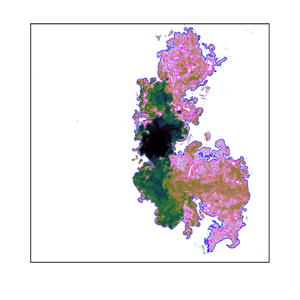
Since the seminal work of Corrsin & Kistler (Reference Corrsin and Kistler1955), the characteristics of the turbulent/non-turbulent interface (TNTI), a thin layer of finite thickness demarcating the outer irrotational ambient from the inner turbulent flow, have been widely studied in jets, wakes, shear layers and boundary layers (e.g. see the review of da Silva et al. Reference da Silva, Hunt, Eames and Westerweel2014). However, the interface between a turbulent ambient and a turbulent flow, that is, the turbulent/turbulent interface (TTI), has scarcely been explored, despite its existence in numerous industrial and environmental applications. The presence of the TTI, across which the vorticity and scalar adjust between the surrounding ambient and the turbulent flow akin to the TNTI layer, was only recently shown for a cylindrical wake in a grid-generated turbulent ambient (Kankanwadi & Buxton Reference Kankanwadi and Buxton2020, Reference Kankanwadi and Buxton2022). The outer boundary of the TTI or the TNTI layer, denoted as ‘outline’ hereafter, is usually detected by applying a low-magnitude threshold to a flow-dependent scalar field (e.g. da Silva et al. Reference da Silva, Hunt, Eames and Westerweel2014). Similar to the TNTI outline, the TTI outline, across which the turbulent entrainment occurs, is also wrinkled over a wide range of scales (figure 1). Turbulent entrainment denotes the ingestion of surrounding fluid (be it turbulent or irrotational) into the main turbulent flow. Entrainment is a multi-scale process (e.g. Sreenivasan, Ramshankar & Meneveau Reference Sreenivasan, Ramshankar and Meneveau1989), with contributions from the smallest scales of the flow (i.e. Kolmogorov microscale) to its largest (e.g. jet width).

Figure 1. Instantaneous scalar concentration ( $\phi$) field of a jet in (a) quiescent ambient (case Q) and in (b) turbulent ambient (case T3) in logarithmic scaling. The outlines and ambient ‘holes’ are shown with the blue and magenta lines, respectively. The coordinate along the outlines is represented by $s$. For the description of cases, see the main text.
The entrainment rate depends on two factors: (i) the propagation velocity of the interface relative to the local fluid motion, or the local entrainment velocity  $v_n$ (e.g. Holzner & Lüthi Reference Holzner and Lüthi2011), and (ii) the surface area of the turbulent interface. For example, compressibility in mixing layers and jets tends to suppress the entrainment rate by reducing the surface area of the interface, while $v_n$ remains relatively unaffected (Jahanbakhshi & Madnia Reference Jahanbakhshi and Madnia2016; Nagata, Watanabe & Nagata Reference Nagata, Watanabe and Nagata2018). The same behaviour was observed due to stratification in gravity currents and shear layers (Krug et al. Reference Krug, Holzner, Lüthi, Wolf, Kinzelbach and Tsinober2015; Watanabe, Riley & Nagata Reference Watanabe, Riley and Nagata2016). Turbulence in the ambient, however, results in a stretched surface area of the TTI outline compared with that of the TNTI outline (figure 1 and § 3.2), which is similar to the increased surface area of a forced temporal wake compared with an unforced one (Bisset, Hunt & Rogers Reference Bisset, Hunt and Rogers2002). That being said, Kankanwadi & Buxton (Reference Kankanwadi and Buxton2020) demonstrated a net reduction of the entrainment rate into their wake from a turbulent background and attributed it to infrequent, but large detrainment events.
Hunt (Reference Hunt1994) argued that any external forcing (e.g. turbulence in the ambient) tending to break up a jet or plume would ultimately result in a decreased entrainment rate. Reduced entrainment was later shown experimentally for a shallow jet in a co-flow (Gaskin, McKernan & Xue Reference Gaskin, McKernan and Xue2004) and more recently for momentum-driven and buoyant jets in approximately homogeneous turbulence (Khorsandi, Gaskin & Mydlarski Reference Khorsandi, Gaskin and Mydlarski2013; Perez-Alvarado Reference Perez-Alvarado2016; Lai, Law & Adams Reference Lai, Law and Adams2019). Sahebjam, Kohan & Gaskin (Reference Sahebjam, Kohan and Gaskin2022) proposed a two-region model for the evolution of a jet in approximately homogeneous turbulence generated by a random jet array (RJA) through a study of its centroidally averaged scalar field. The first region, albeit perturbed by the background turbulence (increased growth rate and concentration decay compared with the quiescent ambient), revealed self-preservation of the centroidally averaged first-order scalar statistics, whilst in the second region, the growth rate ceases and the jet is destroyed. The sudden transition between the two regions was marked by  $\xi = u_{\tau }/u_{jet, q}^{rms} > 0.5$, where $\xi$, $u_{\tau }$ and $u_{jet, q}^{rms}$ denote the relative turbulence intensity between the ambient and the jet, the characteristic velocity of the ambient turbulence and the streamwise ( $x$) root-mean-square (r.m.s.) velocity at the jet centreline in the quiescent ambient, respectively. The latter demonstrates the dominance of the intensity of the background turbulence in defining the behaviour of the shear flow, which renders the length scale of the ambient insignificant in the far field (Kankanwadi & Buxton Reference Kankanwadi and Buxton2020). This is not necessarily valid in the near field due to the dominance of large-scale coherent structures, which increases the importance of the ambient length scale. In any case, our primary interest is in investigating the effect of background turbulence on the interfacial properties of an axisymmetric jet in the far field, for which we substantiate the predominance of the ambient turbulence intensity over its length scale for the cases studied in § 3.
The primary aim of the present work is to assess the geometric features of the TTI outline and compare them with those of the TNTI in an axisymmetric jet. This is important as it will shed light on the turbulent entrainment process between two bodies of rotational flow. To this end, we present a brief description of the experimental set-up (§ 2.1) and mean flow characteristics (§ 2.2). The conditional scalar profiles and the geometric properties of the TTI outline are demonstrated in § 3. Lastly, we conclude with our observations on the effect of background turbulence on the interfacial properties of the jet in § 4.
2. Methodology
2.1. Experimental configuration
The experiments were conducted in a  $1.5 \times 6 \times 1\, \text {m}^{3}$ open-top glass tank. A turbulent jet with a Reynolds number of ${Re}_J = u_e d/\nu = 10\,600$ was produced, where $u_e = 1.25\,\text {m}\,\text {s}^{-1}$ is the jet-exit velocity, $d = 8.51$ mm is the jet diameter and $\nu = 10^{-6}\,\text {m}^{2}\,\text {s}^{-1}$ is the kinematic viscosity of water. A pco.dimax 4 Megapixel CMOS camera equipped with a 50 mm Pentax lens was used for planar laser-induced fluorescence (PLIF) with a field of view (FOV) of $260\times 260\,\text {mm}^{2}$, yielding a resolution of $0.015d$ or $1.7\eta _q$. The centreline Kolmogorov microscale for the jet in a quiescent ambient ( $\eta _q$) is calculated from the empirical relation of Friehe, van Atta & Gibson (Reference Friehe, van Atta and Gibson1971),
 \begin{equation} \eta_q/d = (48 {Re}_J^{3})^{{-}1/4}(x/d), \end{equation}
where subscript  $q$ denotes the quiescent ambient. The measurements were carried out at a downstream station of $x/d = 25$ for all background conditions. Since the focus of the current study is in the vicinity of the TNTI and TTI, the actual resolution is finer as the local Kolmogorov microscale near the interface is approximately 1.5 times larger than its centreline value, as shown in several free-shear flows (e.g. Buxton, Breda & Dhall Reference Buxton, Breda and Dhall2019; Zecchetto & da Silva Reference Zecchetto and da Silva2021). Although the Batchelor microscale is the relevant length scale for assessing the concentration gradients in high-Schmidt flows ( $Sc \gg 1$), the current experimental resolution is sufficient to capture the conditionally averaged mean and r.m.s. scalar profiles along the local normals to the interface (§ 3.1). This is due to the negligible effect of molecular diffusion on the averaged evolution of a high- $Sc$ passive scalar across the interface. Hence, the Kolmogorov microscale is a more suitable normalisation scale near the interfacial layer compared with the Batchelor microscale, when evaluating the conditional mean concentration profiles (see figure 8(a) of Watanabe et al. Reference Watanabe, Sakai, Nagata, Ito and Hayase2015). Additional support is provided by Kohan & Gaskin (Reference Kohan and Gaskin2020), who by coarse graining their PLIF resolution, show that a resolution of approximately 6 $\eta _q$ properly captures the conditionally averaged mean and r.m.s. scalar profiles. The 1.5 mm ( ${\approx }19 \eta _q$) thick laser sheet, formed using an 8-sided polygonal rotating mirror, excited the fluorescent dye (Rhodamine 6G, $Sc \approx 2500$) in the jet. The intensity profiles were converted to concentration values in a calibration process, where absorption of the laser beam during its passage through the dyed fluid was accounted for using the Beer–Lambert law, and corrected along horizontal rows rather than along the actual (oblique) beam path. The maximum error of this procedure was less than 1 %, which occurred at the bottom left corner of the FOV and, thus, was deemed negligible.
The background condition was either quiescent with the RJA being off or turbulent. The turbulent ambient was generated using a RJA with 60 bilge pumps (6 rows and 10 columns; figure 2) with centre-to-centre distance of  $M = 15$ cm. The pumps draw water at their base and discharge it independently from each other, where, downstream of the RJA, their flows merge, creating approximately homogeneous turbulence (as discussed below) without mean shear. The on/off times of the pumps were governed by a ‘random’ algorithm (also known as ‘sunbathing’ algorithm, as proposed in Variano & Cowen Reference Variano and Cowen2008) to simultaneously realise the lowest possible mean flow and the highest degree of homogeneity (Perez-Alvarado Reference Perez-Alvarado2016). The on/off times followed two normal distributions with parameters $(\mu _{{on}}, \sigma _{{on}}) = (12, 4)$ s and $(\mu _{{off}}, \sigma _{{off}}) = (108, 36)$ s, resulting in 10 % of the pumps being on at any instant (on average). The mean flow generated using this algorithm is typically one order of magnitude smaller than the velocity fluctuations (Variano & Cowen Reference Variano and Cowen2008; Perez-Alvarado Reference Perez-Alvarado2016). A cart laterally ( $y$) displaced the RJA sheet, allowing the turbulence intensity and length scale of the RJA turbulence at the jet to be altered, while conducting the measurements at a single downstream station. In addition to the reference quiescent ambient, three turbulent backgrounds were considered at a station prior to the destruction of the jet by ambient turbulence, i.e. $\xi < 0.5$ (Sahebjam et al. Reference Sahebjam, Kohan and Gaskin2022, also table 1), where the distances from the RJA to the jet centreline ( $y/M$) were among those assessed by Perez-Alvarado (Reference Perez-Alvarado2016). This provided the velocity information of the RJA turbulence required to calculate the relative turbulence intensity $\xi = u_{\tau }/u_{jet, q}^{rms}$ and length scale $\mathcal {L} = l_{\tau }/b_{\phi, q}$ between the ambient and the jet. Following Variano & Cowen (Reference Variano and Cowen2008), we define a characteristic ambient velocity $u_{\tau } = (2k_{\tau }/3)^{1/2}$, where $k_{\tau } =1/2[ (u_{RJA}^{rms})_y^{2} + 2(u_{RJA}^{rms})_x^{2} ]$ is the turbulent kinetic energy (TKE) of the ambient at the jet centreline, and is taken from Perez-Alvarado (Reference Perez-Alvarado2016). The calculation of $k_{\tau }$ assumes statistical isotropy of the RJA-generated turbulence in the $x{-}z$ plane, as previously noted by Variano & Cowen (Reference Variano and Cowen2008). The value of $u_{jet, q}^{rms}$ is estimated from Khorsandi et al. (Reference Khorsandi, Gaskin and Mydlarski2013), who used the same experimental apparatus. The integral length scale of the ambient ( $l_{\tau }$) is calculated from the spatial autocorrelation of the streamwise velocity fluctuation of the RJA (Perez-Alvarado Reference Perez-Alvarado2016), while $b_{\phi, q} =$ 21.5 mm is the concentration half-width of the jet in the quiescent ambient. Finally, a characteristic Reynolds number is defined as $\mbox {{Re}}_{\tau } = u_{\tau } l_{\tau }/\nu$, combining the effects of $\xi$ and $\mathcal {L}$ for each turbulent background.

Figure 2. Schematic of the experimental apparatus. (a) Cart for moving the RJA, (b) the RJA plane and pumps, (c) PLIF camera, (d) FOV extent, (e) laser sheet and ( f) laser scanning device, containing the 532 nm continuous laser (1.5 W) and the rotating mirror.
Table 1. Summary of the experimental parameters. Note that  $N_{aq}$, $f_{aq}$ and $\mbox {{Re}}_{\lambda, \tau }$ denote the total number of instantaneous scalar fields, data acquisition frequency and the Taylor Reynolds number of the RJA turbulence, respectively. Here, case Q denotes the jet in quiescent ambient, while cases with the letter T indicate jet in the turbulent ambient.
 $^{a}$The values of $k_{\tau }$ and $l_{\tau }$ in $\mathcal {L} = l_{\tau }/b_{\phi, q}$ are taken from Perez-Alvarado (Reference Perez-Alvarado2016).
It is important to note that, whereas the background turbulence is homogeneous in planes parallel to the RJA after  $y/M > 5$ (Khorsandi Reference Khorsandi2011), its TKE unavoidably decays in the direction normal to the plane of the RJA. This is characteristic of all mono-planar RJA systems, causing inhomogeneity in the direction normal to the plane of the RJA (e.g. see figure 4 of Lai et al. Reference Lai, Law and Adams2019). The homogeneity along this axis (i.e. $y$-axis) can be significantly improved by using a bi-planar RJA system (e.g. Bellani & Variano Reference Bellani and Variano2014; Carter et al. Reference Carter, Petersen, Amili and Coletti2016; Esteban, Shrimpton & Ganapathisubramani Reference Esteban, Shrimpton and Ganapathisubramani2019), due to the underlying symmetric forcing of this experimental set-up. Nonetheless, in Appendix A we show that the characteristic velocity of the ambient, $u_{\tau }$, decays by less than 15 % across the average width of the jet in the worst case scenario (case T3), while the decay of $u_{\tau }$ in the T1 and T2 cases is well below 10 %. A variation of less than 10 %–20 % in turbulence quantities was previously used by Bellani & Variano (Reference Bellani and Variano2014) to identify the spatial extent of the homogeneous region. We, therefore, may be able to claim that the jet is subjected to an approximately homogeneous background turbulence for all the cases considered. Lastly, we emphasise that the characteristics of the background turbulence reported throughout the manuscript were measured in the absence of the axisymmetric jet in the tank.
2.2. Flow characterisation
The radial profiles of mean ( $\bar {\phi }$) and r.m.s. ( $\phi ^{rms}$) concentration normalised by their centreline ( $\phi _c$) and jet-exit ( $\phi _e$) values, and the behaviour of half-width ( $b_{\phi }$) and $\phi _c$ can be appreciated in figure 3. The concentration at a given ( $r, \theta$) is approximated using bilinear interpolation. Thereafter, $\bar {\phi }$ and $\phi ^{rms}$ at a given radial position are calculated as the azimuthally averaged value at that radius at increments of $\theta = 1^{\circ }$. Before presenting the results, we note that the jet in the quiescent ambient has attained first- and second-order scalar self-similarity at $x/d = 25$ (not shown). In accordance with Perez-Alvarado (Reference Perez-Alvarado2016), we find that external forcing tends to radially extend the spatially averaged scalar profile (figure 3a). This can be explained by the increased turbulent diffusion and mean radial velocities near the interface (Khorsandi et al. Reference Khorsandi, Gaskin and Mydlarski2013), resulting in enhanced radial transport of scalar from the jet core towards the edges in the turbulent background. Concurrently, ‘meandering’ of the jet, brought about by the large eddies of the turbulent ambient, can also cause higher average concentrations at large radial distances. Conditioning the average profiles relative to the distance from the interface accounts for the meandering path of the jet (Bisset et al. Reference Bisset, Hunt and Rogers2002) and will, therefore, illustrate the importance of turbulent diffusion in increasing the concentration levels near the jet edge (§ 3.1). The values of $\phi ^{rms}$ increase with increasing relative turbulence intensity (figure 3b; also Perez-Alvarado Reference Perez-Alvarado2016; Sahebjam et al. Reference Sahebjam, Kohan and Gaskin2022), owing to external intermittency, induced by strong meandering, or the combination of external intermittency and the increased scalar fluctuations inside the jet due to the entrainment of external turbulence. Again, the conditional profiles should elucidate the mechanisms governing the increase of $\phi ^{rms}$ in a turbulent ambient. Finally, the increased width of the jet in background turbulence compared with the quiescent ambient is evident from its larger scalar half-width, while the value of $\phi _c$ decreases (figure 3c). Notably, the results presented in this section show the dominance of $\xi$ over $\mathcal {L}$ in characterising the behaviour of the scalar field of a fully developed jet subjected to approximately homogeneous turbulence for the range of relative turbulence intensities and length scales investigated in this study. In particular, the trends of figure 3 follow the hierarchy of $\xi$, even though $\mbox {{Re}}_{\tau }$ is larger for T2 compared with T3.

Figure 3. Effect of external turbulence on the (a) mean and (b) r.m.s. scalar profiles, and on the (c) centreline concentration (closed symbols, left-hand axis) and half-width (open symbols, right-hand axis). The  $y$-axis in the inset plots is normalised with the jet-exit concentration, $\phi _e$, and the error bars in (c) represent the 95 % confidence interval.
As mentioned earlier, figure 3(a,b) depicts the azimuthally averaged mean and r.m.s. concentration profiles, which mask any potential asymmetry of the jet about its centreline in the ambient turbulence. Since the external turbulence is generated only on one side of the jet, the assumption of statistical axisymmetry requires further investigation. In figure 4, we present the contour maps of the mean and r.m.s. concentration fields for the studied cases. We observe that the ensemble-averaged mean and r.m.s. concentration isocontours are slightly shifted towards the RJA (i.e.  $y < 0$) for the turbulent background cases. The slight increase in the spacing of the isocontours for $y<0$ can be ascribed to the slow decay of the background turbulence away from the RJA. However, this minor asymmetry is not significant compared with the mean effect of the background turbulence in the global picture, i.e. external turbulence radially expands the jet region and increases the concentration fluctuations as demonstrated in figure 4.

Figure 4. (a–d) Contour maps of the ensemble-averaged concentration field for the Q, T1, T2 and T3 cases, respectively. (e–h) Same as (a–d) but for the r.m.s. concentration field. The centreline of the jet is shown with the red  $\times$ symbol.
3. Results
3.1. Conditional concentration profiles
We identify the TNTI and TTI outlines by applying a threshold to the instantaneous scalar concentration fields. The algorithm is based on the seminal work of Prasad & Sreenivasan (Reference Prasad and Sreenivasan1989) and is similar to Mistry et al. (Reference Mistry, Philip, Dawson and Marusic2016), that is, a conditional variable is introduced as
 \begin{equation} \tilde{\phi}(\phi_t) = \frac{\varSigma\, (\phi n)|_{\phi>\phi_t}}{\varSigma\, (n)|_{\phi>\phi_t}}, \end{equation}
representing the pixel-averaged concentration value inside the region where the local concentration exceeds a given threshold  $\phi _t$. In the aforementioned relation, $n$ denotes the number of pixels. Figure 5(a) presents the evolution of $\tilde {\phi }$ against a wide range of scalar thresholds for the Q and T3 cases. One can expect $\tilde {\phi }$ to monotonically increase with $\phi _t$, since increasing the threshold would result in highly concentrated regions of passive scalar being identified as the jet. Subsequently, the thresholds corresponding to the TNTI and TTI outlines are found as the inflection points of $\tilde {\phi }$ (figure 5b,c). Because of the high- $Sc$ nature of the passive scalar used in this study (Rhodamine 6G), the primary turbulent shear flow (jet) and the ambient have significantly different levels of concentration, i.e. the scalar boundary separating them is quite ‘sharp’. The detection criterion in figure 5(b,c) utilises this sharpness, that is, the selected thresholds correspond to the slowest change in the value of $\tilde {\phi }$. Thus, one can argue that the changes in the locations of the TNTI and TTI outlines are minimal, provided the thresholds coincide with the local minima of $\text {d}\tilde {\phi }/\text {d}\phi _t$. A similar approach was previously employed by Taveira et al. (Reference Taveira, Diogo, Lopes and da Silva2013) in their direct numerical simulation (DNS) of planar jets, where the vorticity value coinciding with the inflection point of the total ‘turbulent’ volume was chosen as the appropriate threshold. Returning to the current work, the thresholds for the Q, T1, T2 and T3 cases are $\phi _t/\phi _c =$ 0.11, 0.11, 0.13 and 0.14, respectively, where the increasing ratios of the thresholds for increasing $\xi$ implies the existence of higher levels of passive scalar near the interface in the presence of ambient turbulence. The TNTI and TTI outlines are then selected as the longest continuous isocontour along their corresponding $\phi _t/\phi _c$ with instances of ‘islands’ and ‘holes’ excluded. Islands represent the passive scalar pockets with $\phi \geq \phi _t$ that lie outside the main jet body, while holes are regions with $\phi < \phi _t$ inside the jet (figure 1). Due to the strong meandering of the jet in the turbulent ambient, there are instances in which the FOV cannot contain the full extent of the TTI outline. These snapshots, which constitute approximately 3.8 % and 18.3 % of the T2 and T3 cases, respectively, are thus disregarded in the results presented herein. We checked that the discarded data do not alter the main conclusions of the paper as they had an insignificant effect on the results of the analyses. This is further discussed in Appendix C.

Figure 5. (a) Conditional variable  $\tilde {\phi }$ against $\phi _t$ for the Q and T3 cases. (b,c) Gradient of the profiles shown in (a). Black and red dashed lines indicate the inflection points and, thus, the thresholds for the Q and T3 cases, respectively.
The conditionally averaged profiles (denoted by  $\langle \sim \rangle _I$) evaluate the ensemble-averaged flow variables along the local interface-normal coordinate, $\boldsymbol {x_n} = x_n \hat {\boldsymbol {n}}$, where $\hat {\boldsymbol {n}} = \boldsymbol {\nabla }{\phi }/|\boldsymbol {\nabla }{\phi }|$ is the interface-normal unit vector. The jet and the ambient regions are represented by $x_n \geq 0$ and $x_n < 0$, respectively. Following Kohan & Gaskin (Reference Kohan and Gaskin2020), we only consider points along $\boldsymbol {x_n}$ with one flow status change (turbulent or ambient), i.e. we ignore points inside the islands and holes and after an intersection with them. The conditional profiles of mean and r.m.s. concentration presented in figure 6 reveal a steep increase across the finite thickness of the TNTI and TTI layers. The latter attests to the presence of a distinct interfacial region, despite the turbulent background flow. The value of the conditional jumps follows the hierarchy of $\xi$, i.e. greater jumps occur as the turbulence in the ambient is intensified. We note that the different behaviour of the conditionally averaged profiles across different background conditions is not an artefact of the chosen thresholds, since cases Q and T1 possess the same threshold. In addition, we assess the conditional profiles of the T2 and T3 cases using the threshold of the Q and T1 cases of $\phi _t/\phi _c = 0.11$. These are shown with the blue and red dashed lines in figure 6, respectively. Although some changes occur in the profiles, the overall behaviour remains unaltered, that is, greater levels of scalar concentration at the edges of the jet (relative to the values in the jet core) and the enhanced scalar fluctuations in the jet induced by the turbulent ambient cause steeper jumps in $\langle \phi \rangle _I$ and $\langle \phi ^{rms} \rangle _I$, respectively, compared with the jumps in a quiescent ambient. Therefore, jet meandering is not solely responsible for extending the spatially averaged concentration profiles and increasing the spatially averaged r.m.s. concentration in the turbulent ambient, as seen in figures 3 and 4.

Figure 6. Conditional profiles of (a) mean and (b) r.m.s. concentration. The TNTI and TTI outlines ( $x_n = 0$) are shown with the vertical dashed black line. The blue and red dashed lines correspond to the conditional profiles of T2 and T3, respectively, using $\phi _t/\phi _c = 0.11$.
At this point, it is worth noting that the interface defined using a scalar threshold faithfully coincides with that of vorticity when  $Sc \approx 1$ (Gampert et al. Reference Gampert, Boschung, Hennig, Gauding and Peters2014; Watanabe, Zhang & Nagata Reference Watanabe, Zhang and Nagata2018). In contrast, for flows with $Sc$ greater than unity, the scalar interface resides inside its vorticity counterpart due to the weakly diffusive nature of the scalar (e.g. Silva & da Silva Reference Silva and da Silva2017). Specifically, in their DNS of mixing layers with $0.25 \leq Sc \leq 8$ conducted in a quiescent ambient, Watanabe et al. (Reference Watanabe, Sakai, Nagata, Ito and Hayase2015) showed that the jump in the scalar concentration takes place within the finite thickness of the vorticity TNTI, which contains both the viscous superlayer (VSL) and the turbulent sublayer (TSL) (Taveira & da Silva Reference Taveira and da Silva2014; van Reeuwijk & Holzner Reference van Reeuwijk and Holzner2014). More crucially, Watanabe et al. (Reference Watanabe, Sakai, Nagata, Ito and Hayase2015) showed that, for $Sc \gg 1$, such as in the present study, the scalar isosurface appears in the TSL, whose outer boundary divides the regions of high and low vorticity. Hence, the structure of the VSL may not be fully recovered using a high- $Sc$ passive scalar threshold in the quiescent ambient. When, however, background turbulence is present, Kankanwadi & Buxton (Reference Kankanwadi and Buxton2022) concluded that viscosity plays a negligible role within the TTI and that the VSL may not exist at all for cases of intense external turbulence. Here, we are interested in the geometry of the scalar TNTI and TTI outlines, as well as their fractal property, which exists in the inertial range. Therefore, resolving the structure of the VSL is not necessary for our purposes. In short, we confirm that the procedure employed for identifying the scalar threshold is robust as the sharp conditional gradients are captured (further validation of the interface detection methodology is provided in Appendix B). Knowing the thresholds, we now proceed to elicit the effect of background turbulence on the interface geometry.
3.2. The TTI geometry
The geometry of the TNTI and TTI outlines can be characterised by their Euclidean distance from the centreline,  $r_I$, their curvature, $\kappa _I$, the cosine between their radial and normal unit vectors, $\cos (\psi _I)$, their tortuosity, $T_I$, and finally, their fractal dimension, $\beta$. Figure 7(a) presents the probability density function (p.d.f.) of the interface radial position. The p.d.f. of $r_I$ for the jet in the quiescent ambient follows a Gaussian distribution, similar to previous studies (Mistry, Philip & Dawson Reference Mistry, Philip and Dawson2019; Kohan & Gaskin Reference Kohan and Gaskin2020), while the distribution of $r_I$ for the jet in the turbulent ambient increasingly deviates from a Gaussian one due to a large skewness. The wide spans of the TNTI and TTI outline radial positions indicate the large-scale spatial fluctuations of $r_I$, which are increasing with $\xi$. The mean values of the interface radial positions $\overline {r_I}/b_{\phi }$ (shown with dashed lines and provided in the inset of figure 7a) also increase with $\xi$, showing that on average the interface is located further away from the centreline in turbulent ambient.

Figure 7. The p.d.f.s of the (a) interface position, (b) interface curvature and (c) cosine of the interface angle. The mean radial positions in (a) are presented in the inset and shown with vertical dashed lines. The scale of the  $y$-axis in the inset of (b) is linear.
The p.d.f.s of the TNTI and TTI outline curvature can be appreciated in figure 7(b). Since the present outlines are planar curves, their curvature is defined as (Mistry et al. Reference Mistry, Philip and Dawson2019)
 \begin{equation} \kappa_I = \left( \dfrac{\dfrac{\text{d}z}{\text{d}s} \dfrac{\text{d}^{2}y}{\text{d}s^{2}} - \dfrac{\text{d}y}{\text{d}s} \dfrac{\text{d}^{2}z}{\text{d}s^{2}}}{\left[ \left( \dfrac{\text{d} y}{\text{d}s} \right)^{2} + \left( \dfrac{\text{d}z}{\text{d}s} \right)^{2} \right]^{3/2}} \right)_I, \end{equation}
where  $s$ is the distance along the outline in the clockwise direction (figure 1). Using this definition, concave (bulges) and convex (valley) surface elements are identified as $\kappa _I < 0$ and $\kappa _I > 0$, respectively, when looking from the jet region. In Kohan & Gaskin (Reference Kohan and Gaskin2020), it was suggested that the TNTI outline of the orthogonal cross-sections of the jet is dominated by flat concave surface elements (smooth bulges; see figure 1a), while its skewness is towards highly curved concave areas. Figure 7(b) reveals that the most probable curvature for all the background cases is at $\kappa _I d \approx -3$. The TTI outline is also dominated by concave curvature but, more importantly, ambient turbulence reduces the probability of finding points on the TTI outline with zero curvature (i.e. flat surfaces) compared with that of the TNTI. This result indicates that ambient turbulence increases the surface area of the jet. Similarly, Jahanbakhshi & Madnia (Reference Jahanbakhshi and Madnia2016) showed that compressibility in shear layers leads to higher occurrence of zero-curvature points on the TNTI outline, implying that compressibility reduces the surface area of the TNTI. Abreu, Pinho & da Silva (Reference Abreu, Pinho and da Silva2022) also reported the same effect due to viscoelasticity (see their figure 2). Figure 7(b) also indicates that, as the level of relative turbulence intensity increases, the probability of finding highly curved concave surface elements increases, while that of the highly convex boundary points remains relatively unaffected.
The cosine of the interface angle measures the misalignment between the inward radial ( $\hat {\boldsymbol {r}}$) and normal unit vectors of the interface, i.e. $\cos (\psi _I) = \hat {\boldsymbol {r}} \boldsymbol {\cdot } \hat {\boldsymbol {n}}$. As noted in Kohan & Gaskin (Reference Kohan and Gaskin2020), intense corrugation of the interface is characterised by $\cos (\psi _I) \rightarrow -1$, since these interface points radially fold back on themselves (see figure 7 of Kohan & Gaskin 2020). Figure 7(c) shows the effect of ambient turbulence on the interface angle. In particular, external forcing promotes the small-scale wrinkles of the TTI outline compared with that of the TNTI, as indicated by the modification of the orientation of the interface normal from that of the radial unit vector. In other words, the occurrence of points along the interface with $\cos (\psi _I) < 0$ increases with increasing $\xi$.
Tortuosity is another feature of curves, which is often used to measure their level of contortion; the higher the tortuosity value, the more contorted the curve. In the context of turbulent surfaces, Kankanwadi & Buxton (Reference Kankanwadi and Buxton2020) showed that turbulence in the free stream acts to increase the length (and tortuosity) of the interface in cylindrical wakes. We define jet tortuosity,  $T_I$, as
 \begin{equation} T_I = L_I/2{\rm \pi}\overline{r_I}, \end{equation}
where  $L_I$ is the interface length for each instantaneous field, calculated as the summation of the Euclidean distance between consecutive points along the TNTI and TTI outlines. Note that all the outlines are closed curves, as those not fully contained within the FOV were discarded. Figure 8(a) displays the p.d.f.s of the TNTI and TTI outline tortuosity. It is evident that the mean effect of the background turbulence is to lower the peak and widen the p.d.f.s, resulting in a more tortuous interface. Similar to the previously described interfacial properties, the mean tortuosity $\overline {T_I}$ is also governed by $\xi$ rather than $\mbox {{Re}}_{\tau }$ (figure 8b). Kankanwadi & Buxton (Reference Kankanwadi and Buxton2020) also reported the relative turbulence intensity as the primary factor in increasing the tortuosity of the TTI outline compared with that of the TNTI in the fully developed region of a cylindrical wake exposed to free-stream turbulence.

Figure 8. (a) The p.d.f.s of the interface tortuosity for different background conditions. (b) Mean tortuosity against relative turbulence intensity. The dashed line and error bars in (b) represent the best linear regression fit and the 95 % confidence interval, respectively.
The multi-scale nature of the turbulent entrainment process can be described using the fractal property of the TNTI and TTI outlines. The fractal property of turbulent surfaces states that their area or their length in two-dimensional planar sections can be scaled as a function of the measurement resolution (Sreenivasan et al. Reference Sreenivasan, Ramshankar and Meneveau1989). It is quite common to spatially filter the interface length to obtain its one-dimensional (1-D) fractal exponent (e.g. Mistry et al. Reference Mistry, Philip, Dawson and Marusic2016), yielding  $\overline {L_I}(\varDelta _f) \propto \varDelta _f^{-\beta }$, where $\varDelta _f$ and $\beta$ and are the box-averaging filter width and the 1-D fractal exponent, respectively. Invoking the Reynolds number similarity, Kolmogorov scaling and Mandelbrot's additive law (Mandelbrot Reference Mandelbrot1982) leads to a universal value of $\beta = 1/3$ for turbulent surfaces. We proceed by convolving each instantaneous concentration field according to $\hat {\phi } = \int \phi (\boldsymbol {x} - \boldsymbol {x}') G(\boldsymbol {x}')\, \text {d}^{2}\boldsymbol {x}'$, with $\hat {\phi }$ and $G$ representing the low-pass filtered concentration field and the box-averaging filter kernel of width $\varDelta _f$, respectively. The TNTI and TTI outlines at each filter width are then identified by applying the same thresholds as for their unfiltered cases. Figure 9(a) presents the pre-multiplied interface length with $\varDelta _f^{1/3}$ for each background condition as a function of the filter width. Visually, a flat line is achieved for the jet in the quiescent ambient, while the pre-multiplied interface length for the jet subjected to the most extreme ambient turbulence intensity (i.e. T3) slightly deviates from a flat line. This is made evident by comparing the profiles with the green horizontal lines in figure 9(a). This implies that background turbulence alters the fractal exponent of the interface, albeit marginally. In order to better examine the evolution of $\beta$ in background turbulence, the negative of the local slope of the filtered interface length, $-\text {d}[ \text {log} ( \overline {L_I}) ]/\text {d}[\text {log}(\varDelta _f)]$, is provided in figure 9(b). Approximate plateaus can be observed for each case, whose heights are slightly increasing with relative turbulence intensity, i.e. the value of $\beta$ is an increasing function of $\xi$. In particular, the fractal exponent increases to $\beta = (0.34 \pm {0.02})$ in the T1 and T2 cases, and to $\beta = (0.35 \pm {0.02})$ in the T3 case within the plateau. This is in agreement with an increased magnitude of the fractal exponent of wakes subjected to free-stream turbulence (Kankanwadi & Buxton Reference Kankanwadi and Buxton2020). The increased magnitude of $\beta$ is in accordance with previous observations presented herein, indicating the more intense corrugation of the TTI outline compared with that of the TNTI, which ultimately results in the strong increase of the interfacial surface area (Krug et al. Reference Krug, Holzner, Marusic and van Reeuwijk2017) in the presence of external turbulence.

Figure 9. (a) Pre-multiplied interface length as a function of the filter width. (b) Local slopes of the filtered interface length. Note that  $\beta$ in (b) is calculated from the approximate plateau region, delimited by the vertical dashed lines.
4. Conclusions
We have experimentally examined the effect of zero-mean-flow approximately homogeneous background turbulence of different intensities on the interfacial properties of an axisymmetric jet. The ambient turbulence is created using a RJA. We confirm that external forcing radially extends the spatially averaged concentration profile and increases the value of the spatially averaged r.m.s. concentration at any given radial position (Perez-Alvarado Reference Perez-Alvarado2016). The averaged scalar statistics, conditioned by their distance from the interface, reveal steeper interfacial jumps in a turbulent ambient compared with those in a quiescent ambient, irrespective of the threshold value. This is attributed to the enhanced transport of scalar from the jet core towards the interface and the increased scalar fluctuations within the jet induced by background turbulence. Turbulence in the ambient impacts the geometric statistics of the interface across all length scales, i.e. the widening of the p.d.f. of the interface radial position is evidence of the turbulent background's large-scale modulation, while the reduction in the occurrence of the zero-curvature surface elements and the modification of the alignment between the normal and radial unit vectors of the interface suggest boundary modulation at smaller scales. The increased wrinkling of the boundary by the turbulent ambient also manifests as an increase in tortuosity and as slightly larger fractal exponents compared with the quiescent background. We show that, for the cases studied here ( $0.15 \leqslant \xi \leqslant 0.26$ and $3.5 \leqslant \mathcal {L} \leqslant 5.5$), the aforementioned changes caused by the background turbulence are primarily governed by the relative turbulence intensity between the ambient and the fully developed jet, rendering the length scale of the ambient relatively unimportant. It is, however, essential to note that the dominance of $\xi$ over $\mathcal {L}$ in the far field of the jet may not hold for much larger or smaller values of ambient length scales (i.e. $\mathcal {L} \ll 1$ or $\mathcal {L} \gg 1$). Further investigation on this matter seems warranted.
Lastly, given the similarity of the present findings regarding a round jet subjected to RJA-generated turbulence to those of Kankanwadi & Buxton (Reference Kankanwadi and Buxton2020) in a different free-shear flow (i.e. cylindrical wake exposed to grid-generated turbulence), we may cautiously hint at the universality of the influence of free-stream turbulence on the geometric properties of the TTI outline. Any such claim, however, entails rigorous experiments using a large range of Reynolds numbers and turbulent flows.
Funding
The authors graciously acknowledge the financial support provided by the Natural Sciences and Engineering Research Council of Canada discovery grant (No. RGPIN 2016-04473).
Declaration of interests
The authors report no conflict of interest.
Appendix A. Comments on the decay of the RJA turbulence normal to its plane
Variano & Cowen (Reference Variano and Cowen2008) and Lai et al. (Reference Lai, Law and Adams2019) showed that the TKE and r.m.s. velocity components of the RJA turbulence exhibit a power-law decay in the direction normal to the RJA plane after the initial merging zone. This can be seen in figure 10, where the velocity information is adopted from Perez-Alvarado (Reference Perez-Alvarado2016). Note that Perez-Alvarado (Reference Perez-Alvarado2016) measured the turbulence statistics of the RJA at an additional lateral location of  $y/M = 6.7$, which is included in figure 10 to improve the robustness of the exponential fits.

Figure 10. Evolution of various statistics of the background turbulence against the distance from the RJA plane. The region delimited by the vertical lines represent the average width of the jet for each case. The black dashed lines are the exponential best fits to the velocity statistics, while the black dot-dashed lines show the lateral position of the jet centreline relative to the RJA.
The level of inhomogeneity across the jet is estimated by considering the mean position of the TTI outline in each case. Recall that  $\overline {r_I}/b_{\phi } =$ 1.84, 2.02 and 2.37 for the T1, T2 and T3 cases, respectively, as presented in figure 7(a). In combination with the half-width values in figure 3(c), we find that, on average, the jet occupies a region of width $0.543 M\, (9.6 d)$, $0.599 M\, (10.6 d)$ and $0.789 M\, (13.9 d)$, for the T1, T2 and T3 cases (we checked that the radial position of the TTI outline is approximately symmetric about the jet centreline). Knowing the power-law fits and the average boundaries of the jet, we estimate that the characteristic velocity of the ambient decays by 5.7 %, 8.1 % and 13.5 % across the jet in the T1, T2 and T3 cases, respectively. Furthermore, we found weak correlation between the interface geometry and the azimuthal angle ( $\theta$) in the turbulent background (not shown), which attests to the fact that the slow decay of the RJA turbulence does not systematically affect the interfacial properties on different sides of the jet. Hence, it is safe to say that the jet is experiencing a somewhat ‘homogeneous’ external turbulence in all cases for our purposes.
Appendix B. Validation of the interface detection methodology
In order to assess the validity of the concentration-based threshold approach, utilised to detect the TNTI and TTI outlines in § 3.1, we compare it with the method explained in Kankanwadi & Buxton (Reference Kankanwadi and Buxton2020). The new method involves applying a threshold to the modulus of the fluorescent signal (intensity) gradient, taken from the 12-bit camera. The modulus of the intensity gradient is preferred to that of the intensity itself due to the presence of a ‘halo’ effect, surrounding the highly concentrated local passive scalar blobs. This phenomenon originates from the secondary excitation of the localised patch of dye by the fluorescent light emitted in its close proximity (e.g. Vanderwel & Tavoularis Reference Vanderwel and Tavoularis2014; Baj, Bruce & Buxton Reference Baj, Bruce and Buxton2016).
The approach is the same as that described in § 3.1, that is, a new scalar field is introduced as  $\varPhi = \lvert \boldsymbol {\nabla } I \lvert$, where $I$ is the corrected fluorescent signal of the camera. The correction procedure includes subtraction of the mean background intensity (when no concentration is present) from the raw intensity matrix, followed by applying a median filter to account for the single-pixel objects. A median filter is further applied to the resulting $\lvert \boldsymbol {\nabla } I \lvert$ fields to smooth out some of the non-physical large values associated with experimental noise (e.g. bubble entering the FOV), and to ease the detection of $\lvert \boldsymbol {\nabla } I \lvert _t$ as detailed below. We then define the conditional intensity gradient modulus as
 \begin{equation} \widetilde{\left| \boldsymbol{\nabla} I \right|} = \dfrac{\varSigma\, (\left| \boldsymbol{\nabla} I \right|\, n)|_{\left| \boldsymbol{\nabla} I \right|>\left| \boldsymbol{\nabla} I \right|_t}}{\varSigma\, (n)|_{\left| \boldsymbol{\nabla} I \right|>\left| \boldsymbol{\nabla} I \right|_t}}, \end{equation}
and determine the threshold as the value of  $\left | \boldsymbol {\nabla } I \right |$ which coincides with the inflection point of $\widetilde {\left | \boldsymbol {\nabla } I \right |}$. The validity of this method depends on the gradual variation of light intensity in the background, i.e. we assume that ambient possesses relatively small values of intensity gradient, while the jet region is characterised by high values of $\widetilde {\left | \boldsymbol {\nabla } I \right |}$ due to its dynamic condition.
Figure 11(a) depicts the behaviour of  $\widetilde {\left | \boldsymbol {\nabla } I \right |}$ for the Q and T3 cases. Although less clear for the T3 case, plateaus exist in $\widetilde {\left | \boldsymbol {\nabla } I \right |}$ corresponding to a range of thresholds for which $\widetilde {\left | \boldsymbol {\nabla } I \right |}$ changes slowly. Inflection points are identified at $\left | \boldsymbol {\nabla } I \right |_t$ = 30 for both cases, marking the threshold for the scalar isocontours. Figure 11(b,c) displays the conditionally averaged mean and r.m.s. concentration along local normals to the interface detected with the concentration threshold (open symbols) and that detected with the intensity gradient modulus threshold (filled symbols). Whilst some discrepancy exists between the two methods, sharp jumps are evident at $x_n = 0$ for $\langle \phi \rangle _I$ and $\langle \phi ^{rms} \rangle _I$, indicating that the mean location of the interface is similar for both detection methodologies. We also checked that the trends in $\langle \phi \rangle _I$ and $\langle \phi ^{rms} \rangle _I$ for different background cases (i.e. steeper jumps for increasing $\xi$) do not change with the new interface detection procedure. Thus, we conclude that the scalar concentration is a robust marker for the TNTI and TTI outlines in the current study.

Figure 11. (a) Evolution of  $\widetilde {\left | \boldsymbol {\nabla } I \right |}$ as a function of the scalar threshold, $\left | \boldsymbol {\nabla } I \right |_t$, for the Q and T3 cases. The vertical dashed line at $\left | \boldsymbol {\nabla } I \right |_t = 30$ indicates the inflection point of the profiles. Conditionally averaged profiles of (b) mean and (c) r.m.s. concentration for the $\phi$-isocontour (open symbols) and $\left | \boldsymbol {\nabla } I \right |$-isocontour (filled symbols).
Appendix C. Comments on the effect of the discarded data
We carried out additional analyses to evaluate the influence of the discarded scalar concentration fields on the interfacial properties for the T2 and T3 cases. Recall that approximately 4 % of the T2 and 18 % of the T3 case realisations were removed from the analyses due to the limited size of the FOV. The data cleaning was deemed appropriate, as information regarding the interface points outside the FOV was lost. This in turn could bias the geometric features of the remaining TTI outline points in that instantaneous field. Nonetheless, comparing the results using the complete datasets with those in § 3 revealed minor differences in the conditional mean and r.m.s. profiles, as well as the interface curvature and angle (figures not shown for brevity). However, one can expect the average radial position and length of the TTI outline to increase when the disregarded data are considered.
In figure 12(a), we show the p.d.f.s of the TTI outline radial position for the cleaned up (solid lines) and complete (dashed lines) datasets. The left tails of the distributions remain similar for both datasets in each case, whereas the right tails, which present far radial locations from the centreline, become wider when the discarded data are included. Consequently, the values of  $\overline {r_I}/b_{\phi }$ are greater for the complete datasets compared with those of the corrected ones. The same behaviour is observed for the p.d.f.s of the TTI outline tortuosity in figure 12(b), i.e. the left tails remain approximately identical, while the occurrence of high tortuosity events (right tails) increases for the complete datasets. We, however, note that the simultaneous increase in the radial location and length of the interface cause $\overline {T_I}$ to only slightly increase when the discarded fields are considered. Lastly, we present the local slopes of the filtered TTI outline length in figure 12(c) for the corrected and complete datasets. Although the interfaces are ‘rougher’ on average upon inclusion of the discarded data, the fractal dimensions are unaltered, that is, $\beta = 0.34 \pm 0.02$ and $\beta = 0.35 \pm 0.02$ for the T2 and T3 cases, respectively, independent of the number of instantaneous scalar fields. To conclude, the disregarded datasets do not influence the main trends observed in the interfacial properties of a jet subjected to external turbulence and jet meandering is chiefly correlated with the large-scale geometric characteristics of the interface (e.g. radial location).

Figure 12. Influence of the discarded snapshots on the p.d.f.s of the TTI outline (a) radial position, (b) tortuosity and on the value of the (c) fractal exponent for the T2 (blue) and T3 (red) cases. The results using the complete data are shown with the dashed lines, while the solid lines represent the cleaned up data used in § 3. The vertical solid and dashed lines in (a) are the mean radial locations of the TTI outlines. The region between the vertical dashed lines in (c) presents the approximate scaling range, similar to figure 9.


 Open access