


1. Introduction
Unbalanced motions are a prevalent feature of the upper ocean driven by unrelenting atmospheric forcing, most notably in the form of wind stresses and surface heat fluxes. These motions often take the form of near-inertial oscillations, horizontal motions that oscillate at or near the inertial frequency  $f = 2\varOmega \sin {\lambda }$ where
  $\varOmega$ is the angular velocity of the Earth, and
  $\lambda$ is the latitude. In addition, atmospheric forcing can give rise to a slew of dynamic instabilities especially in the submesoscale regime, characterised by Rossby numbers, the ratio of relative to planetary vorticity, and balanced Richardson numbers, the square of the ratio of buoyancy frequency to geostrophic shear, of order unity (Thomas, Tandon & Mahadevan Reference Thomas, Tandon and Mahadevan2008; McWilliams Reference McWilliams2016). Submesoscale instabilities can be categorised broadly by the structure of the perturbations and their energy source.
At fronts, wind-induced frictional forces or diabatic cooling (Thomas Reference Thomas2005) can drive a change in sign of the Ertel potential vorticity (PV)  $q$, such that
  $fq < 0$, resulting in symmetric instability (SI) (Hoskins Reference Hoskins1974). SI and the extended family of inertia-symmetric instabilities that form in stably stratified flows are primarily shear instabilities that draw from a reservoir of kinetic energy. For pure SI, kinetic energy is extracted through geostrophic shear production from the ‘thermal wind’ that balances the lateral buoyancy gradients that define fronts (Thomas et al. Reference Thomas, Taylor, Ferrari and Joyce2013). SI is characterised by two-dimensional (2-D) overturning cells, aligned with isopycnals and invariant in the along-front direction. Alternatively, fronts stable to this class of instabilities may undergo a baroclinic instability (Stone Reference Stone1966, Reference Stone1970; Boccaletti, Ferrari & Fox-Kemper Reference Boccaletti, Ferrari and Fox-Kemper2007). Baroclinic instabilities draw from the reservoir of potential energy stored in the lateral density gradient. These instabilities are a major contributor to the rich field of eddies that are found in the submesoscale regime (Callies et al. Reference Callies, Flierl, Ferrari and Fox-Kemper2016). Both classes of submesoscale instability are associated with ageostrophic circulations that not only restratify the upper ocean but also transport heat, momentum, and biogeochemically important tracers between the air–sea interface and interior ocean.
In this paper, we describe a different submesoscale instability that occurs at unbalanced fronts. It is closely related to SI but draws from the kinetic energy of the unbalanced motions rather than the geostrophic flow. We extend the analysis of Thomas & Taylor (Reference Thomas and Taylor2014), henceforth referred to as T&T, which introduced a new damping mechanism on vertically sheared inertial oscillations at fronts, namely parametric subharmonic instability (PSI). As with SI, baroclinic effects are the underlying driver of this instability. Lateral buoyancy gradients reduce the minimum frequency of inertia-gravity waves and increase the perturbation slope at which the minimum is achieved (Whitt & Thomas Reference Whitt and Thomas2013). T&T found that at fronts with a sufficiently small balanced Richardson number, such that the minimum frequency of inertia-gravity waves is less than  $f/2$, vertically sheared inertial oscillations are unstable to PSI. Importantly, PSI can occur when
  $fq \geq 0$, thus the presence of unbalanced motions at fronts extends the region of instability.
The analytical results of T&T focused on along-isopycnal perturbations that, in the hydrostatic limit and under the assumption of weak inertial shear, correspond to inertia-gravity waves with the lowest frequency since they do not create a buoyancy anomaly. They are therefore the most unstable modes near the critical value of the balanced Richardson number. Here, we derive a formulation of the linear stability analysis that does not require this restriction, nor does it require that the perturbations be in hydrostatic balance. In doing so, we extend the parameter space to which these results are applicable.
In particular, relaxing the hydrostatic constraint allows us to consider fronts that are instantaneously unstratified and thus capture a range of geostrophic adjustment problems. The prototypical example of this is a lateral buoyancy gradient following a storm where buoyancy and momentum are well mixed in the vertical. The resulting flow consists of transient sheared inertial oscillations about a steady equilibrium state (Tandon & Garrett Reference Tandon and Garrett1994). The equilibrium state is partially restratified but unstable to mixed-layer instability, a type of baroclinic instability, that restratifies the front further (Fox-Kemper, Ferrari & Hallberg Reference Fox-Kemper, Ferrari and Hallberg2008). However, we are interested in the damping of the transient oscillations. Viscous effects are always active in dampening the unbalanced flow, and at finite-width fronts, the inertial oscillations may propagate away. Here, we show that the inertial oscillations are additionally unstable to PSI, leading to a potentially more rapid dampening of the transient flow.
Here, we consider the stability of an idealised model of inertial shear at an infinite uniform front. We begin, in § 2, by deriving governing equations for the perturbations in a coordinate system advected with the isopycnals. With a plane wave assumption, these are reduced to a pair of coupled ordinary differential equations in time, which we solve numerically to find the Floquet exponents and periodic eigenfunctions. In § 3, we introduce a 2-D nonlinear numerical model and compare the predictions of the linear theory to numerical simulations. The nonlinear evolution of the simulations once the perturbations reach finite amplitude, including the onset of secondary Kelvin–Helmholtz instabilities and the damping of the inertial shear, is described in § 4. Then in § 5, we consider the final state of the simulations once the flow has restabilised, and the changes to the balanced front induced by the instabilities. Finally, we provide conclusions and discussion in § 6.
2. Linear stability analysis
2.1. Background state
We use the same background state as T&T, an infinite front under a sheared inertial oscillation (figure 1). The front has constant horizontal buoyancy gradient  $-\partial B/\partial y = S^2$, which is balanced by geostrophic shear. The inertial shear is also spatially uniform, and the resulting background flow is an exact solution to the Boussinesq equations on an
  $f$-plane. The horizontal velocities and stratification
  $\partial B/\partial z = N^2$ are given by
 $$\begin{gather} U = \frac{S^2}{f}\left(1 - \delta\,{{Ri}}\cos (\,ft)\right)z, \end{gather}$$
 $$\begin{gather}V = \delta\,{{Ri}}\,\frac{S^2}{f}\sin (\,ft)\,z , \end{gather}$$
 $$\begin{gather}N^2 = N_0^2(1 - \delta\cos (\,ft)). \end{gather}$$
There is no vertical velocity, and the pressure is hydrostatic. The balanced Richardson number of the front is
 \begin{equation} {{Ri}} := \frac{N_0^2f^2}{S^4}, \end{equation}
and  $\delta$ is a scaling factor that determines the strength of the inertial shear. Unlike T&T, who included the initial phase of the inertial oscillation as a free parameter, we prefer to express the problem in terms of the balanced, or mean, state, and have chosen a particular phase with the stratification initially minimal. This phase choice is ideal for studying the ‘classic geostrophic adjustment problem’ of Tandon & Garrett (Reference Tandon and Garrett1994). However, the stability of this set-up is independent of the choice of initial phase.

Figure 1. Schematic of the background flow and coordinate systems for  ${{Ri}} = 4/3$,
  $\delta = 3/4$,
  $\varGamma = 10$ when
  $ft = {\rm \pi}/2$. Isopycnals are contoured in black, isolines of absolute momentum in grey, and the across- and along-front velocities are indicated in red and blue, respectively.
While the stratification varies as isopycnals are sheared by the ageostrophic flow, the PV
 \begin{equation} q := \left(\,f\hat{\boldsymbol{z}} + \boldsymbol{\nabla}\boldsymbol{\wedge} \boldsymbol{u}\right)\boldsymbol{\cdot}\left(\boldsymbol{\nabla}b\right) = fN^2 -S^2\,\frac{\partial U}{\partial z} = fN_0^2 - \frac{S^4}{f} \end{equation}
is conserved. Here and in § 2.2,  $\boldsymbol {u} = (u,v,w)$ is the velocity,
  $b$ is the buoyancy,
  $\boldsymbol {\nabla } = (\partial /\partial x, \partial /\partial y, \partial /\partial z)$ is the gradient operator, and
  $\boldsymbol {\wedge }$ indicates a cross-product. In the absence of inertial shear, the minimum frequency for hydrostatic inertia-gravity waves is given by
 \begin{equation} \omega_{min} = \sqrt{\frac{fq}{N_0^2}} = f\,\sqrt{1 - {{Ri}}^{-1}} \end{equation}
(Whitt & Thomas Reference Whitt and Thomas2013). For weak ageostrophic shear, we expect – and T&T found – that the flow is unstable to PSI when  $\omega _{min} < \tfrac {1}{2}f$,
  ${{Ri}} < \tfrac {4}{3}$, and unstable to SI when
  $\omega _{min}^2 < 0$,
  ${{Ri}} < 1$. Here, we extend the analysis of T&T to include not only arbitrary perturbations, but a larger range of parameter space where non-hydrostatic effects will become important. In particular, we consider stronger inertial shears applicable to geostrophic adjustment. Two special cases of geostrophic adjustment are
  $\delta = {{Ri}}^{-1}$ and
  $\delta = 1$. These correspond to initial conditions with well-mixed momentum and buoyancy, respectively. Their intersection
  ${{Ri}} = \delta = 1$ corresponds to the ‘classic geostrophic adjustment problem’.
2.2. Governing equations in an advected coordinate system
Our governing equations are the non-hydrostatic, inviscid, adiabatic, Boussinesq equations on an  $f$-plane:
 $$\begin{gather}
\frac{\mathrm{D}\boldsymbol{u}}{\mathrm{D}t} +
f\hat{\boldsymbol{z}}\boldsymbol{\wedge} \boldsymbol{u} +
\boldsymbol{\nabla}p - b\hat{\boldsymbol{z}} = 0,
\end{gather}$$
$$\begin{gather}
\frac{\mathrm{D}\boldsymbol{u}}{\mathrm{D}t} +
f\hat{\boldsymbol{z}}\boldsymbol{\wedge} \boldsymbol{u} +
\boldsymbol{\nabla}p - b\hat{\boldsymbol{z}} = 0,
\end{gather}$$ $$\begin{gather} \frac{\mathrm{D}b}{\mathrm{D}t} = 0,\end{gather}$$
 $$\begin{gather} \boldsymbol{\nabla}\boldsymbol{\cdot} \boldsymbol{u} = 0. \end{gather}$$
We, like T&T, will consider only perturbations with across-front variability, thereby effectively precluding baroclinic instabilities. We explicitly set the x derivatives to zero, but retain all three components of the velocity. The material derivative is  ${\rm D}/{\rm D}t=\partial/\partial t+v \partial/\partial y+w\partial/\partial z$ and p is the pressure divided by the Boussinesq reference density.
In this 2-D inviscid adiabatic set-up, both the buoyancy and along-front momentum equations can be written in conservative form. We define the absolute momentum  $M = u - fy$, and write the along-front momentum equation as
  $\mathrm {D}M/\mathrm {D}t = 0$. The absence of along-front derivatives reduces the PV to the Jacobian of
  $b$ and
  $M$,
$M$,  $q = J(b,M) = |\partial (b,M)/\partial (y,z)|$, and its conservation follows from the conservation of
  $b$ and
  $M$. The absolute momentum of the background flow is
  $U - fy = f^{-1}S^2(1 - \delta \,{{Ri}}\cos ft)z - fy$, and the background buoyancy is
  $B = B_0 - S^2y + N_0^2(1 - \delta \cos {ft})z$. This motivates a new non-dimensional coordinate system advected with the isopycnals, which we denote by tildes (figure 1). Define
 \begin{equation} \tilde{y} := \frac{1}{L}\left(y - \frac{N_0^2}{S^2}\,(1 - \delta\cos{ft})z\right), \end{equation}
where  $L$ is, at this point, an arbitrary horizontal length scale. Defining the front strength
 \begin{equation} \varGamma := \frac{S^2}{f^2}, \end{equation}
which may take either sign but from here on will be assumed to be positive, the background buoyancy is 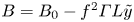 $B = B_0 - f^2\varGamma L\tilde {y}$. We use
  $f$ to non-dimensionalise time,
  $\tilde {t} := ft$, and the horizontal across-isopycnal velocity in the advected coordinate system is given by
 \begin{align} \tilde{v} := \frac{1}{f}\,\frac{\mathrm{D}\tilde{y}}{\mathrm{D}t} = \frac{v}{fL} - \frac{N_0^2}{S^2}\left(\delta\sin{ft}\,\frac{z}{L} + (1 - \delta\cos{ft})\,\frac{w}{fL}\right) = \frac{v - V}{fL} - \frac{N_0^2}{S^2}\,(1 - \delta\cos{ft})\,\frac{w}{fL}, \end{align}
where the inertial oscillations of the background flow drop out naturally. Identifying a frequently appearing aspect ratio
 \begin{equation} \gamma := \frac{S^2}{N_0^2} = \varGamma^{-1}{{Ri}}^{-1} \end{equation}
defined by the balanced isopycnal slope, the natural along-isopycnal coordinate is  $\tilde {z} := z/\gamma L$, with corresponding velocity
 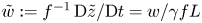 $\tilde {w} := f^{-1}\,\mathrm {D} \tilde {z}/\mathrm {D}t = w/\gamma fL$. Finally, we define non-dimensional along-front momentum, buoyancy and pressure perturbations:
 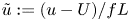 $\tilde {u} := (u - U)/fL$,
 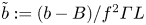 $\tilde {b} := (b - B)/f^2\varGamma L$,
  $\tilde {p} := (\,p - P)/f^2L^2$, where
  $P = P_0 + (B_0 -S^2y)z + N_0^2z^2/2$ is the background pressure. Under these transformations, the governing equations become
 $$\begin{gather} \frac{\mathrm{D}\tilde{u}}{\mathrm{D}\tilde{t}} - \tilde{v} + ({{Ri}}^{-1} - 1)\tilde{w} = 0, \end{gather}$$
 $$\begin{gather}\frac{\mathrm{D}\tilde{v}}{\mathrm{D}\tilde{t}} + (1 - \delta\cos\tilde{t})\,\frac{\mathrm{D}\tilde{w}}{\mathrm{D}\tilde{t}} + \tilde{u} + \frac{\partial\tilde{p}}{\partial\tilde{y}} + 2\delta\sin\tilde{t}\tilde{w} = 0, \end{gather}$$
 $$\begin{gather}\gamma^2\,\frac{\mathrm{D}\tilde{w}}{\mathrm{D}\tilde{t}} + \frac{\partial\tilde{p}}{\partial\tilde{z}} - (1 - \delta\cos\tilde{t})\,\frac{\partial\tilde{p}}{\partial\tilde{y}} - {{Ri}}^{-1}\,\tilde{b} = 0, \end{gather}$$
 $$\begin{gather}\frac{\mathrm{D}\tilde{b}}{\mathrm{D}\tilde{t}} - \tilde{v} = 0 , \end{gather}$$
 $$\begin{gather}\frac{\partial\tilde{v}}{\partial\tilde{y}} + \frac{\partial\tilde{w}}{\partial\tilde{z}} = 0, \end{gather}$$
where  $\mathrm {D}/\mathrm {D}\tilde {t} = \partial /\partial \tilde {t} + \tilde {v}\,\partial /\partial \tilde {y} + \tilde {w}\,\partial /\partial \tilde {z}$ is the material derivative in the advected coordinate system.
In this coordinate system, the total buoyancy and absolute momentum take on very simple forms with constant uniform background gradients. The total buoyancy is given by  $\tilde {b} - \tilde {y}$, and the absolute momentum transforms to
  $\tilde {M} = \tilde {u} - \tilde {y} + ({{Ri}}^{-1} - 1)\tilde {z}$, where the inertial variability has been absorbed into the coordinate definition. Furthermore, the governing equations for the perturbations are independent of the new spatial coordinates.
The stability problem is described by three non-dimensional parameters: the balanced Richardson number  ${{Ri}}$, the strength of the inertial shear
  $\delta$, and implicitly the front strength
  $\varGamma$ through the aspect ratio
  $\gamma$. Note that we are considering parameter ranges with
  ${{Ri}} = O(1)$, hence
  $\gamma \sim \varGamma ^{-1}$. However,
  $\gamma$ and hence
  $\varGamma$ influence the solutions only through the non-hydrostatic acceleration, so we expect the solutions to have negligible dependence on
  $\varGamma$ in large parts of parameter space.
2.3. Plane wave solution
In this coordinate system, we look for plane wave solutions
 \begin{equation} \left[\tilde{u},\tilde{v},\tilde{w},\tilde{b},\tilde{p}\right]^{\rm T} = \left[\hat{u}(t),\hat{v}(t),\hat{w}(t),\hat{b}(t),\hat{p}(t)\right]^{\rm T} \exp({\mathrm{i}(\tilde{y}-\alpha_0\tilde{z})}) + \mathrm{c.c.}, \end{equation}
where we have dropped the tilde on  $t$ for convenience, and taken the horizontal wavenumber to be 1. This fixes a choice for the previously arbitrary length scale
  $L$, which we assume implicitly is large enough to justify the inviscid adiabatic assumption.
Defining  $\alpha (t) = 1 + \alpha _0 -\delta \cos t$ and using the continuity equation to eliminate
  $\hat {v}$, we have
 $$\begin{gather} \frac{\mathrm{d}\hat{u}}{\mathrm{d}t} - (1 + \alpha_0 - {{Ri}}^{-1})\hat{w} = 0 , \end{gather}$$
 $$\begin{gather}\alpha(t)\,\frac{\mathrm{d}\hat{w}}{\mathrm{d}t} + \hat{u} +\mathrm{i} \hat{p} + 2\delta\sin t\hat{w} = 0, \end{gather}$$
 $$\begin{gather}\gamma^2\,\frac{\mathrm{d}\hat{w}}{\mathrm{d}t} - \mathrm{i}\,\alpha(t)\,\hat{p} - {{Ri}}^{-1}\,\hat{b} = 0, \end{gather}$$
 $$\begin{gather}\frac{\mathrm{d}\hat{b}}{\mathrm{d}t} - \alpha_0\hat{w} = 0. \end{gather}$$
Multiplying (2.12b) by  $\alpha (t)$, adding (2.12c), and defining the along-isopycnal displacement amplitude
  $\zeta$ such that
  $\mathrm {d}\zeta /\mathrm {d}t = \hat {w}$,
  $\hat {b} = \alpha _0\zeta$ and
  $\hat {u} = (1 + \alpha _0 - {{Ri}}^{-1})\zeta$, reduces these equations to
 \begin{equation} \frac{\mathrm{d}}{\mathrm{d}t}\left[\left(\alpha(t)^2 + \gamma^2\right)\hat{w}\right] = \left(\alpha_0\,{{Ri}}^{-1} - (1 + \alpha_0 - {{Ri}}^{-1})\,\alpha(t)\right)\zeta. \end{equation}
Finally defining  $\varPsi = (\alpha (t)^2 + \gamma ^2)\hat {w}$, we arrive at a pair of coupled ordinary differential equations:
 $$\begin{gather} \frac{\mathrm{d}\varPsi}{\mathrm{d}t} = \left(\alpha_0\,{{Ri}}^{-1} - (1 + \alpha_0 - {{Ri}}^{-1})\,\alpha(t)\right)\zeta , \end{gather}$$
 $$\begin{gather}\frac{\mathrm{d}\zeta}{\mathrm{d}t} = \left(\alpha(t)^2 + \gamma^2\right)^{-1}\varPsi. \end{gather}$$
The coefficients of (2.14) are periodic and time reversible. We can therefore use Floquet theory to write any given solution as
 \begin{equation} \begin{bmatrix}\varPsi(t) \\ \zeta(t)\end{bmatrix} = A\,\mathrm{e}^{\mu t} \begin{bmatrix}\varPsi_1(t) \\ \zeta_1(t)\end{bmatrix} + B\,\mathrm{e}^{-\mu t} \begin{bmatrix}\varPsi_2(t) \\ \zeta_2(t)\end{bmatrix} \end{equation}
for some  $A$ and
  $B$, where
  $\varPsi _1$,
  $\zeta _1$,
  $\varPsi _2$ and
  $\zeta _2$ are periodic eigenfunctions (Floquet Reference Floquet1883). By integrating forwards two linearly independent initial conditions, we find the Floquet exponents
  $(\mu,-\mu )$, with
  $\mathrm {Im} (\mu ) \in (-1/2,1/2]$, and corresponding eigenfunctions (see Appendix A for details). Note that we do not consider the degenerate cases with
  $\mu = -\mu$, which may be avoided by the inclusion of viscosity. The system (2.14) displays a further symmetry under complex conjugation, denoted by superscript
  $*$, therefore we must have
  $\mu ^* = \mu$ or
  $\mu ^* = -\mu$. The latter implies purely imaginary Floquet exponents and corresponds to stable wavelike solutions. The former can be split into two cases where without loss of generality we take
  $\mathrm {Re} (\mu ) > 0$. First, for
  $\mu$ real, we have one decaying and one growing solution. This is the case that includes SI. Second, since the imaginary part of the Floquet exponent is defined modulo
  $1$, we can have
  $\mu \in \{a + 1/2\mathrm {i} \, | \, a \in \mathbb {R}, \ a > 0 \}$. This growing oscillatory behaviour at the subharmonic frequency characterises PSI and allows us to distinguish between PSI modes and SI modes (figure 2). In all cases, we define the growth rate
  $\sigma = \mathrm {Re} (\mu )$.

Figure 2. Plots of (a) growth rate  $\sigma$, and (b)
  $\alpha _0$, for the most unstable solutions for
  $\varGamma = 10$. Black contours bound the region where the imaginary parts of the Floquet exponents were
  $1/2$, indicating PSI. Grey dashed lines indicate the special cases
  $\delta = {{Ri}}^{-1}$ and
  $\delta = 1$. Black stars, labelled in (b) by simulation number, indicate the initial conditions of simulations SIM01–13.
2.4. Physical interpretation
In physical space, the structure of the perturbations is  $\exp (\mathrm {i}(y - \gamma ^{-1}\,\alpha (t)\,z)/L)$, and their slope is
  $\gamma \,\alpha (t)^{-1}$. The horizontal wavenumber is fixed, but the vertical wavenumber varies sinusoidally. This observation allows us to interpret the system of (2.14) as a coupling between the along-front vorticity and the thermal wind imbalance. Multiplying (2.13) by
  $\mathrm {i}\gamma ^{-2}$, we have
 \begin{align} \frac{\mathrm{d}}{\mathrm{d}t}\left[-\left(\gamma^{-2}\,\alpha(t)^2 + 1\right)\frac{\hat{w}}{\mathrm{i}}\right] = \gamma^{-1}\left(\mathrm{i}\gamma^{-1}\,{{Ri}}^{-1}\,\alpha_0 - \mathrm{i}\gamma^{-1}\,\alpha(t)\,(1 + \alpha_0 - {{Ri}}^{-1})\right)\zeta. \end{align}
Then introducing a streamfunction  $\tilde {\phi } = \hat {\phi } \exp ({\mathrm {i}(\tilde {y}-\alpha _0\tilde {z})}) + \mathrm {c.c.}$, such that
  $\hat {w} = \mathrm {i}\hat {\phi }$, and rewriting the right-hand side in terms of
  $\hat {u}$ and
  $\hat {b}$, we get
 \begin{equation} \frac{\mathrm{d}}{\mathrm{d}t}\left[-\left(1 + \gamma^{-2}\,\alpha(t)^2\right)\hat{\phi}\right] = \gamma^{-1}\left(\mathrm{i}\varGamma \hat{b} - \mathrm{i}\gamma^{-1}\,\alpha(t)\,\hat{u}\right). \end{equation}
Unwrapping our coordinate transformation, we interpret this equation as the creation of along-front vorticity  $\phi _{yy} + \phi _{zz}$ by the thermal wind imbalance
  $f^{-1}b_y + u_z$ (Thomas, Lee & Yoshikawa Reference Thomas, Lee and Yoshikawa2010).
2.5. Growth rate and perturbation slope
The region of instability for PSI extends out from the critical value  $4/3$ of the balanced Richardson number in the limit of vanishing inertial shear (figure 2). As
  $\delta$ increases, so does the critical value of
  ${{Ri}}$, denoted
  ${{Ri}}_{c}(\delta )$, for which the flow is unstable to PSI. For balanced Richardson numbers smaller than
  ${{Ri}}_{c}$, the flow is unstable. The fastest growing modes are PSI modes if
  ${{Ri}} \gtrapprox 1$, and SI modes if
  ${{Ri}}$ is smaller. Note that there is a small region with
  ${{Ri}} < 1$ where PSI modes grow faster than SI modes. The growth rate
  $\sigma$ in the PSI regime depends strongly on the strength of the inertial shear
  $\delta$, weakly on the balanced Richardson number
  ${{Ri}}$, and negligibly on
  $\varGamma$ unless
  $\delta \approx 1$. The growth rate of SI, on the other hand, increases rapidly with
  ${{Ri}}^{-1}$, but also increases with increasing
  $\delta$. In the absence of inertial shear, the growth rate of SI is given by
 \begin{equation} \sigma_{SI} = \sqrt{{{Ri}}^{-1} - 1} \end{equation}
for  ${{Ri}} < 1$. In weak inertial shear, the growth rates of PSI are modest. However, in strong inertial shear, of order the thermal wind shear,
  $\delta = {{Ri}}^{-1}$, growth rates
  $\sigma \approx 1/2$ are achievable. For context,
  $\sigma _{SI} = 1/2$ when
  ${{Ri}} = 4/5$. Increasing
  $\delta$ further increases the growth rate. The physically realisable limit for inertial shear is
  $\delta \approx 1$, after which the front periodically becomes negatively stratified with the inertial oscillations advecting dense water over light. In this part of parameter space, we find
  $O(1)$ growth rates that depend on
  $\varGamma$ (figure 3).

Figure 3. Growth rate  $\sigma$ and
  $\alpha _0$ for the special cases (a,b)
  $\delta = {{Ri}}^{-1}$, (c,d)
  $\delta = 1$, and (e,f)
  $\delta = {{Ri}} = 1$ as functions of
  $\varGamma$.
The free parameter  $\alpha _0$ defines the slope of perturbations in the advected coordinate system. Here,
  $\alpha _0 = 0$ describes an along-isopycnal perturbation, and consequently both
  $\tilde {v}$ and
  $\tilde {b}$ are zero. Also,
  $\alpha _0 > 0$ describes perturbations that are shallower than the isopycnal slope, and
  $\alpha _0 < 0$ describes perturbations that are steeper. Isolines of absolute momentum are given by
  $\alpha _0 = {{Ri}}^{-1} - 1$. As
  ${{Ri}}^{-1}$ increases, so does
  $\alpha _0$. There is a transition across which the solution changes from being almost exactly along-isopycnal,
  $|\alpha _0| \ll 1$, to shallower than isopycnals,
  $\alpha _0 \approx 1$. In weak inertial shear,
  $\delta \ll 1$, this is explained by the requirement for the solutions to have frequency
  $f/2$. As
  ${{Ri}}^{-1}$ increases, the minimum frequency – that is, the frequency of along-isopycnal perturbations – decreases, and in order to obtain the required phasing, the solutions must be increasingly off-isopycnal. As
  $\delta$ increases and the solution amplitudes are deformed from perfect sinusoids, the fastest growing modes become more along-isopycnal. For shallow slopes
  $|\alpha (t)| \gg \gamma$, the hydrostatic approximation is valid and the problem becomes independent of the front strength
  $\varGamma$. PSI in weak inertial shear is well described by the hydrostatic regime for
  $\varGamma \gg 1$,
  $N_0 \gg f/2$. In this region of parameter space, the growth rate should be independent of
  $\varGamma$. It was this regime that was considered in T&T. However, for stronger inertial shear and the initially unstratified geostrophic adjustment problem (
 $\delta = 1$), non-hydrostatic effects can be important, with the front strength playing a role in setting the growth rate. The dependence on
  $\varGamma$ for the two special cases
  $\delta = {{Ri}}^{-1}$ and
  $\delta = 1$ is explored in figure 3. We find that in the former, there is little dependence on
  $\varGamma$ unless
  ${{Ri}}^{-1} = \delta \approx 1$. This is because the fastest growing modes occur for
  $\alpha _0 \approx 0$ and hence the condition for
  $\alpha (t) \approx \gamma$ is that
  $\delta \approx 1$.
More interesting is the case  $\delta = 1$, where the background state periodically becomes instantaneously unstratified. Here, the growth rates of the fastest growing modes with
  $\alpha _0 \approx 0$ grow with increasing
  $\varGamma$ and are not well described by the hydrostatic assumption. However, the classic geostrophic adjustment problem with
  ${{Ri}} = \delta = 1$ is the exception, as
  $\alpha _0 = 0$ is stable. When
  ${{Ri}} = 1$, the coefficient in (2.14a) is proportional to
  $\alpha _0$. Consequently, as
  $\varGamma \to \infty$,
  $\alpha _0$ takes on a finite value with
  $\gamma \ll \alpha _0$, and the growth rate asymptotes. The asymptotic value is
  $1/2$ and is achieved approximately for
  $\varGamma > 100$, values which are typical of observed ocean fronts (e.g. Sarkar et al. Reference Sarkar, Pham, Ramachandran, Nash, Tandon, Buckley, Lotliker and Omand2016). However, large buoyancy gradients occur, in general, only at narrow fronts or low latitudes, hence our uniform,
  $f$-plane front model may be a poor approximation.
Finally, for small  ${{Ri}}^{-1}$, we find an instability with growth rates comparable to PSI. In addition to PSI, it is possible to excite solutions corresponding to higher harmonics of the subharmonic, that is, solutions with frequency
  $nf/2$. Most of the unstable region at small
  ${{Ri}}^{-1}$ below the PSI regime in figure 2 corresponds to the excitation of inertial solutions or more precisely solutions where the Floquet exponents are real and the periodic eigenfunctions have two zero crossings. Note that at fronts where the minimum frequency is subinertial, there are two inertial characteristics, one horizontal and one steep, and here we are exciting a solution along the steep characteristic. Unlike PSI, the excitation of the higher harmonics occurs only at strictly finite
  $\delta$. Furthermore, the regions of instability, as a function of
  $\alpha _0$, are relatively narrow, and the steeper perturbations are more susceptible to viscous damping, a claim justified by the analysis presented in § 3.3. Therefore, we prefer to focus on the PSI and SI modes.
2.6. Energetics of the linear solutions
Both PSI and SI are primarily shear instabilities in that they grow by extracting energy from the background flow through shear production. However, considering even the simplest case of along-isopycnal perturbations, the energy source is different. We define the phase-averaged perturbation kinetic energy as
 \begin{equation} E_{\hat{k}} := |\hat{u}|^2 + |\hat{v} + (1-\delta\cos{t})\hat{w}|^2 + \gamma^2|\hat{w}|^2, \end{equation}
which satisfies the evolution equation
 \begin{align} \frac{1}{2}\,\frac{\mathrm{d}E_{\hat{k}}}{\mathrm{d}t} = \underbrace{-{{Ri}}^{-1}|\hat{u}\hat{w}^*|}_{\text{GSP}} + \underbrace{\delta\cos{t}|\hat{u}\hat{w}^*| - \delta\sin{t}\,|(\hat{v} + (1-\delta\cos{t})\hat{w})\hat{w}^*|}_{\text{AGSP}} + \underbrace{{{Ri}}^{-1}|\hat{w}\hat{b}^*|}_{\text{BF}}. \end{align}
We identify three different production terms: the geostrophic shear production (GSP), the ageostrophic shear production (AGSP), and the buoyancy flux (BF). The relative contributions of these three terms to the change in perturbation kinetic energy over an inertial period was calculated to identify the dominant sources of perturbation kinetic energy (figure 4). PSI grows by extracting energy from the ageostrophic shear, whereas SI, which can be active in the absence of ageostrophic shear, extracts its energy primarily from the geostrophic shear. However, SI will also access the ageostrophic shear, and as the ageostrophic shear increases, it accounts for a larger fraction of the total. By contrast, the fastest growing PSI modes have negative GSP. PSI modes are very efficient at extracting energy from the ageostrophic shear, although the off-isopycnal modes supplement the AGSP with a buoyancy flux and thus extract potential energy from the background state.

Figure 4. Relative contributions to the growth in perturbation kinetic energy from (a) geostrophic shear production (GSP), (b) ageostrophic shear production (AGSP), and (c) buoyancy fluxes (BF), over one inertial period for  $\varGamma = 10$. The boundary between PSI and non-PSI modes is denoted by black contours determined by the imaginary part of the Floquet exponents. The special cases of geostrophic adjustment
  $\delta = {{Ri}}^{-1}$ and
  $\delta = 1$ are denoted by grey dashed lines.
The time dependence of the background flow and growing solutions result in an interesting phase dependence in energetics. This phasing also depends on the strength of the inertial shear. In very weak inertial shear, we can build intuition by considering the PSI modes as inertia-gravity waves with frequency  $1/2$. Note that this argument can be formalised with the method of multiple scales by introducing a slow time scale
  $\delta ^{-1}t$. The inertia-gravity waves are propagating across-front, hence
  $\tilde {v}$ and
  $\tilde {w}$ are in phase and in quadrature with
  $\tilde {u}$ and
  $\tilde {b}$. Therefore,
  $|\hat {u}\hat {w}^*|$ and
  $|\hat {w}\hat {b}^*|$ integrate to zero over the course of an inertial period, and the only term that contributes to the growth is the second term in the ageostrophic shear production. Consider an along-isopycnal mode such that
  $\tilde {v} = 0$. In this case, the change in perturbation kinetic energy over an inertial period is
 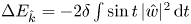 $\Delta E_{\hat {k}} = -2\delta \int \sin {t}\,|\hat {w}|^2\,\mathrm {d}t$. The optimal phasing for growth is
  $\hat {w} \sim \cos (t/2 + {\rm \pi}/4)$, and the growth is maximal when
  $t = 3{\rm \pi} /2$. We find that as the inertial shear is increased, the phase of the maximum growth shifts later in the inertial period towards the phase when the stratification is weakest. We can draw an analogy to SI in the presence of inertial shear where shear production is enhanced during the phases when the stratification is weakening (Thomas et al. Reference Thomas, Taylor, D'Asaro, Lee, Klymak and Shcherbina2016; Wienkers, Thomas & Taylor Reference Wienkers, Thomas and Taylor2021b).
3. Numerical simulations
We use 2-D nonlinear simulations to verify the findings of the preceding linear stability analysis and explore the decay of the inertial shear. The simulations were run with DIABLO, a non-hydrostatic hydrodynamics code (Taylor Reference Taylor2008). DIABLO solves the Boussinesq equations on an  $f$-plane, employing a uniform staggered grid with second-order finite differences in the vertical, and a collocated pseudo-spectral method in the periodic horizontal direction(s). The equations are stepped forward using a third-order-accurate implicit–explicit scheme with an adaptive time step.
3.1. Simulation design
To simulate a front, we utilise the ‘frontal zone’ set-up, as in Taylor & Ferrari (Reference Taylor and Ferrari2009), where the simulation is made periodic by subtracting a uniform horizontal buoyancy gradient and the corresponding geostrophic shear. We solve for the ageostrophic flow, including terms in the governing equations that capture the advection of the subtracted geostrophic momentum and buoyancy. We neglect the along-front variations running 2-D simulations with sufficient resolution to resolve secondary Kelvin–Helmholtz (KH) instabilities. We use a small viscosity  $\nu$ so as not to damp the inertial oscillations before the PSI modes have a chance to develop. However, in the simulations that we ran with Laplacian viscosity (not shown), we found that this damping is insufficient to avoid a pile-up of energy at the grid scale at certain times during the simulations, hence we choose to employ a hyper-viscosity for the horizontal damping. It should be noted that we find the results presented here to be insensitive to the choice of horizontal damping, under resolved Laplacian versus hyper-viscosity.
Unfortunately, DIABLO requires a new non-dimensionalisation. We use the domain half-height  $H$, the geostrophic shear
  $f\varGamma$, and the corresponding advective velocity scale
  $f\varGamma H$, to non-dimensionalise lengths, time and velocities. The buoyancy is non-dimensionalised by
 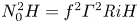 $N_0^2H = f^2\varGamma ^2{{Ri}} H$. From here on, unless explicitly stated, it should be assumed that all derivations and calculations are with respect to this non-dimensionalisation. Importantly, the parameters
  ${{Ri}}$ and
  $\varGamma$ are exactly as defined before. The model solves the following equations:
 $$\begin{gather} \frac{\partial \boldsymbol{u}}{\partial t} + \boldsymbol{u}\boldsymbol{\cdot}\boldsymbol{\nabla} \boldsymbol{u} + w\hat{\boldsymbol{x}} + \frac{1}{\varGamma}\,\hat{\boldsymbol{z}}\boldsymbol{\wedge} \boldsymbol{u} + \boldsymbol{\nabla}p - {{Ri}}\,b \hat{\boldsymbol{z}} = \frac{{{Ek}}}{\varGamma}\left[\frac{\partial^2}{\partial z^2} - \nu_H\,\frac{\partial^4}{\partial y^4}\right]\boldsymbol{u}, \end{gather}$$
 $$\begin{gather}\frac{\partial b}{\partial t} + \boldsymbol{u}\boldsymbol{\cdot}\boldsymbol{\nabla}b - \frac{1}{{{Ri}}\,\varGamma}\,v = \frac{{{Ek}}}{\varGamma}\left[\frac{\partial^2}{\partial z^2} - \nu_H\,\frac{\partial^4}{\partial y^4}\right] b , \end{gather}$$
 $$\begin{gather}\boldsymbol{\nabla}\boldsymbol{\cdot} \boldsymbol{u} = 0. \end{gather}$$
The initial conditions are given by
 \begin{equation} u =-\delta_0\,{{Ri}}\,z, \quad v = 0, \quad w = 0, \quad b = (1-\delta_0)z, \end{equation}
plus white noise of amplitude  $10^{-4}$ in the velocity fields, which are then projected onto a divergence-free subspace. These initial conditions correspond exactly to the background state (2.1) with
  $\delta = \delta _0$. The top (
 $z=1$) and bottom (
 $z=-1$) boundary conditions relax the solution to the balanced state:
 \begin{equation} \frac{\partial u}{\partial z} = \frac{\partial v}{\partial z} = 0, \quad w = 0, \quad \frac{\partial b}{\partial z} = 1. \end{equation}
These boundary conditions are designed to minimise the drag on the inertial oscillations due to the boundaries. We use a fixed Ekman number  ${{Ek}} := \nu /(\,fH^2) = 10^{-3}$, with the exception of SIM15, and the resulting decay of the inertial oscillations at the start of the simulations is small. The horizontal damping utilises a hyper-viscosity to effectively dissipate the energy at the smallest scales. The hyper-viscosity was adjusted manually, and a scaling factor
  $\nu _H = 4(LY/NY)^4/(LZ/NZ)^2$ was found to work in all cases. Here,
  $LY$ is the non-dimensional domain width, and
  $LZ = 2$ is the non-dimensional domain height. Also,
  $NY$ is the number of grid points in the horizontal – however, in order to dealias the quadratic nonlinearities, the spectral resolution is
  $\lfloor NY/3\rfloor$ Fourier modes;
  $NZ$ is the number of grid points in the vertical.
3.2. Validation of the linear theory
We conducted a coarse sweep of parameter space involving 13 simulations (SIM01–13 in table 1, black stars in figure 2). However, here we focus on results from a single simulation, SIM07. For these parameter values,  $Ri^{-1} = \delta = 0.75$, the linear theory predicts approximately along-isopycnal PSI modes with dimensional growth rate
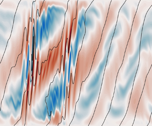
  $0.37f$. The simulation captures the exponential growth of PSI shear bands and the tilting of the isopycnals by the background flow as well as the onset of secondary instability at around 13 inertial periods (figure 5). Qualitatively, the linear theory holds and we observe the growth of large horizontal wavelength PSI modes that are slightly shallower than the isopycnals. However, the slopes of the perturbations are too shallow compared to those predicted by the linear theory, and we can also see some features of the solution associated with the boundary conditions that are not considered in the linear theory. Most notably, the vertical velocity is required to vanish at the top and bottom boundaries, and there is some evidence of reflected perturbations (e.g. figure 5a).
Table 1. Predicted and observed growth rates,  $\sigma$ and
  $\alpha _0$ values, for a coarse sweep of parameter space with
  $\varGamma = 10$. Superscript (lin) and (sim) denote values from the linear theory, using
  $\delta = \delta _0$, and the simulations, respectively. All simulations were run for 20 inertial periods with
  $NZ = 481$,
  $NY = 8192$ and
  ${{Ek}} = 10^{-3}$, with the exception of SIM15. In SIM15,
  ${{Ek}} = 5\times 10^{-4}$,
  $NZ = 993$ and
  $NY=16384$ were used. This simulation was stopped after 6.5 inertial periods, which was sufficient to determine the growth rate and
  $\alpha _0$. For simulations SIM01–13, the width of the domain was
  $LY = 4\varGamma \,{{Ri}}$. The simulation growth rate was inferred from the perturbation kinetic energy, and
  $\alpha _0$,
  $\delta$ from a fit to the perturbation slope as described in § 3.2. Missing values are from simulations in which perturbations did not grow or grew too slowly to allow for a good fit.


Figure 5. Sections of the across-front shear  $v_z$ (
 $\,f\varGamma$) from SIM07. The colour scale is a symmetric log scale, linear between
  $\pm 0.1$, that captures the exponential growth in the amplitude of the PSI modes. Contours of the total buoyancy are overlaid in black with spacing
  $0.4f^2\varGamma ^2\,{{Ri}}\,H$.
To study and quantify properties of the PSI modes, in particular the theoretical predictions for the growth rate and perturbation slope, we decompose the ageostrophic fields into a lateral mean, the inertial oscillations denoted by overbars (e.g.  $\overline {u}$), and perturbations from that mean denoted by primes (
 $u'$). Plotting the perturbation kinetic energy
  $E_{k,{p}} := \tfrac {1}{2}\left \langle \boldsymbol {u}'\boldsymbol {\cdot } \boldsymbol {u}'\right \rangle$ where
  $\langle {\cdot }\rangle$ denotes a domain average, as a function of time (figure 6a), we determine the growth rate of the perturbations to be
  $0.18f$, approximately half of the theoretical value. The growth rates across all the simulations were significantly, but not uniformly, reduced from the theoretical prediction (table 1). Nonetheless, in strong inertial shear, growth rates of
  $f/3$ were achieved.

Figure 6. Evolution of (a) the perturbation kinetic energy, and (c) the dominant perturbation slope for simulation SIM07. The plot in (a) is a semilog plot of the perturbation kinetic energy, with a linear fit in log space overlaid in dashed red. The theoretical inviscid growth rate is indicated by the blue dashed line. We identify the dominant slope of the perturbations by considering the autocorrelation of  $u'$ (red) and
  $v'$ (blue) as a function of displacement angle, or equivalently
  $\alpha$, and then fit the expected form
  $\alpha = 1 + \alpha _0 - \delta \cos (t/\varGamma )$, as described in § 3.2. The fraction of variance unexplained (FVU, which is
  $1-\rho$) for the dominant slope is plotted in (b), and the inferred
  $\alpha$ is plotted in (c). The weighted linear least squares fit is overlaid in black.
The linear theory also predicts the slope of the perturbations to be  $\gamma \,\alpha (t)^{-1}$, where in non-dimensional simulation time,
  $\alpha (t) = 1 + \alpha _0 - \delta \cos (t/\varGamma )$. The aim of the following analysis is to extract the value of
  $\alpha _0$ that best describes the perturbations in each simulation before finite-amplitude effects play a significant role in the dynamics.
We wish to find the slopes of the lines of constant phase, therefore we consider spatial autocorrelations of the along-front,  $u'$, and across-front,
  $v'$, perturbation velocities. We first calculate the autocorrelations, e.g.
  $R_{u'}$, as a function of the displacement
  $\boldsymbol {r} := (\Delta y,\Delta z)$:
 $$\begin{gather} R_{u'}(\boldsymbol{r}) := \frac{1}{\left\langle u'^2\right\rangle}\,\frac{1}{\left|S(\boldsymbol{r})\right|}\sum_{\mathcal{S}(\boldsymbol{r})}u'(y_1,z_1)\,u'(y_2,z_2), \end{gather}$$
 $$\begin{gather}\mathcal{S}(\boldsymbol{r}) := \{y_1,y_2,z_1,z_2 \, | \, y_2-y_1 \equiv \Delta y\ \text{mod}\ {NY}, z_2-z_1=\Delta z\}, \end{gather}$$
where  $\mathcal {S}(\boldsymbol {r})$ is the set of all pairs of points in the domain separated by
  $\boldsymbol {r}$, accounting for the periodicity in
  $y$. Here,
  $|S(\boldsymbol {r})|$ is the size of the set, which depends on the vertical displacement
  $\Delta z$. Next, we bin these autocorrelations according to the angle of the displacement vector. Defining
  $\theta := \tan ^{-1}(\gamma \,\Delta y/\Delta z)$, we create 200 uniformly spaced bins over the range
  $0 < \theta \leq {\rm \pi}$. Note that the autocorrelations are symmetric under
  $\boldsymbol {r} \to -\boldsymbol {r}$, allowing us to limit the range of
  $\theta$. Then we define
  $\rho _{u'}(\theta )$ by taking the mean of
  $R_{u'}(\boldsymbol {r})$, weighted by
  $|S(\boldsymbol {r})|$, for each bin. This gives us the autocorrelation as a function of the displacement angle
  $\theta$, and therefore
  $\alpha$ since
  $\alpha = \cot {\theta }$.
We use the  $\theta$ that maximises
  $\rho _{u'}(\theta )$ to infer the dominant perturbation slope. We plot both
  $1 - \rho _{u'}$, which we can interpret as the fraction of variance unexplained (FVU) by the assumption that the perturbations are perfectly correlated along the given slope, and the
  $\alpha$ value at the maxima,
  $\alpha _{u'}$, as a function of time (figure 6c). We see that the predicted sinusoidal time dependence of
  $\alpha$ is realised, but with periodic outliers. These outliers are coincident with times when the FVU is large, and occur when the amplitude of the dominant PSI mode is approximately zero. We calculate
  $\alpha _{v'}$ in the same way; it displays similar behaviour, but the outliers occur at a different inertial phase, which is to be expected as
  $u'$ and
  $v'$ should not be in phase.
To extract  $\alpha _0$, we do a two-parameter (
 $\alpha _0$ and
  $\delta$) linear regression to the expected form
  $\alpha (t) = 1 + \alpha _0 - \delta \cos (t/\varGamma )$, during the exponentially growing phase. To mitigate bias from the outliers, we fit
  $\alpha _{u'}$ and
  $\alpha _{v'}$ together, and weight the fit by
  $1/(1-\rho _{u'})$ and
  $1/(1-\rho _{v'})$ as appropriate. The inferred
  $\alpha _0$ and
  $\delta$ values for all the simulations where PSI modes grew sufficiently to dominate the perturbations are listed in table 1 alongside the predictions from the linear theory. We fit for
  $\delta$ in addition to
  $\alpha _0$ as the background inertial oscillations are decaying viscously. Nevertheless, the inferred
  $\delta$ values are close to their initial values, with the best agreement for the fastest growing modes as the fits were taken over the shortest intervals and hence there was less opportunity for viscous decay. The decay of the inertial shear is considered in more detail in § 4.2. Of more interest is the noticeable discrepancy between the simulations and the theory in the value of
  $\alpha _0$. With the exception of SIM03, the observed perturbations are shallower and more across-isopycnal than the theoretical predictions. Potentially, this has significant consequences for the energetics of the perturbations as the buoyancy flux will play a larger role than predicted by the linear theory.
3.3. Viscosity and geometric constraints
Viscous effects are the most obvious source of the observed discrepancies, and we find that the inclusion of viscosity in the linear theory, combined with the geometric constraints of the domain, explains not only the slower growth rates but also the shallower slope of the fastest growing perturbations. While deriving the viscous theory, we return to the advected coordinate system and variables defined in § 2.2.
The derivation of (2.14) is largely unchanged by the inclusion of viscosity; we merely gain a few extra terms. Adding a vertical Laplacian operator  $\nu \,\partial ^2/\partial z^2$ to the Boussinesq momentum and buoyancy equations (assuming Prandtl number 1 as in the simulations), (2.14) becomes
 $$\begin{gather} \frac{\mathrm{d}\varPsi}{\mathrm{d}t} = \left(\alpha_0\,{{Ri}}^{-1} - (1 + \alpha_0 - {{Ri}}^{-1})\,\alpha(t)\right)\zeta - {{Ek}}_{wave}\,\alpha(t)^2\,\varPsi, \end{gather}$$
 $$\begin{gather}\frac{\mathrm{d}\zeta}{\mathrm{d}t} = \left(\alpha(t)^2 + \gamma^2\right)^{-1}\varPsi - {{Ek}}_{wave}\,\alpha(t)^2\,\zeta, \end{gather}$$
where 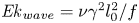 ${{Ek}}_{wave} = \nu \gamma ^2l_0^2/f$ is an Ekman number defined using the horizontal wavenumber, and
  $\zeta$ is no longer exactly the along-isopycnal displacement but still satisfies
  $\hat {u} = (1+\alpha _0 - {{Ri}}^{-1})\zeta$ and
  $\hat {b} = \alpha _0\zeta$. Here, the dimensional horizontal wavenumber
  $l_0 = L^{-1}$, which dropped out of the original derivation, plays an important role in setting the strength of the damping. While it is intuitive that the damping will reduce the growth rate and preferentially select larger wavelength perturbations, it is not obvious why the slope of the perturbations is affected. To explain this, we must also consider geometric constraints.
The finite size of the numerical domain discretises the permitted horizontal wavelengths and vertical modes. Although the horizontal wavelength influences  ${{Ek}}_{wave}$ directly, we find that in our simulations, the vertical constraint is more influential in setting the perturbation slope. We can see this by comparing simulations SIM14 to SIM07, and simulations SIM16–18 to SIM11–13. The only differences between these simulations are the domain widths, and we find the same growth rates and perturbation slopes. However, there are differences at finite amplitude for the simulations with
  ${{Ri}} \approx 1$, which are discussed in § 4.3. The vertical constraint necessarily requires a deviation from the linear theory that considers tilting plane waves that not only fail to satisfy the boundary condition on the vertical velocity but also have a continuous variation in the vertical wavenumber. Nonetheless, we can make some inferences about the impact of viscosity by observing that a common feature of the simulations is that the vertical wavelength, at the inertial phase when it is maximal, approximately fills the domain. This behaviour is observed frequently in simulations of SI (e.g. Bachman & Taylor Reference Bachman and Taylor2014). However, the time dependence of the vertical wavelength means that we should expect the damping to be stronger than that of an SI mode with the same Ekman number.
Imposing a constraint on the maximum vertical wavelength  $\lambda _{max}$, we explore what this means for the damping coefficient:
 \begin{equation} m_{min} = \frac{2{\rm \pi}}{\lambda_{max}} = \gamma l_0\,\alpha(0) \implies \gamma l_0 = \frac{\rm \pi}{H(1 + \alpha_0 - \delta)}\,\frac{2H}{\lambda_{max}}, \end{equation}
where in the final expression we have multiplied and divided by  $H$, the domain half-height, so that we can apply this theory directly to the simulations. Substituting this into the expression for the time-dependent viscous damping coefficient
 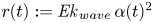 $r(t) := {{Ek}}_{wave}\,\alpha (t)^2$ gives
 \begin{align} r(t) = {\rm \pi}^2\,{{Ek}}\left(\frac{\lambda_{max}}{2H}\right)^{-2}\frac{(1 + \alpha_0 - \delta\cos t)^2}{(1 + \alpha_0 - \delta)^2} = {\rm \pi}^2\,{{Ek}}\left(\frac{\lambda_{max}}{2H}\right)^{-2}\left[1 + \delta\,\frac{1-\cos t}{1 + \alpha_0 - \delta}\right]^2, \end{align}
where  ${{Ek}} := \nu /fH^2$ is the Ekman number used in the simulations. We see that increasing
  $\alpha _0$ reduces the damping, hence we might expect the optimal
  $\alpha _0$ to be larger than that predicted by the inviscid theory. We allow for flexibility in the maximum vertical wavelength, and suggest only that
  $\lambda _{max}/2H \approx 1$. In particular, we do not require
  $\lambda _{max}/2H \leq 1$. Finally, we define the effective Ekman number
  ${{Ek}}_{eff} := {{Ek}}(\lambda _{max}/2H)^{-2}$.
Armed with this expression for the damping, we can solve the system (3.5) for the viscous growth rate and optimal  $\alpha _0$. These results for
  ${{Ri}}^{-1} = \delta = 0.75$ and
  $\varGamma = 10$ (SIM07) are shown in table 2 for different
  ${{Ek}}_{eff}$. Furthermore, we plot curves of the growth rate against
  $\alpha _0$ (figure 7). The simulation growth rate and
  $\alpha _0$ are best described by the calculation with
  ${{Ek}}_{eff} = 2\times 10^{-3}$. For
  ${{Ek}} = 10^{-3}$, as in the simulation, this corresponds to maximum vertical wavelength
  $\sqrt {2}\,H$. Furthermore, we ran a simulation (SIM15) with the same parameters as SIM07 except that we reduced the Ekman number by a factor of 2. We find that the growth rate and
  $\alpha _0$ match with the calculation for
  ${{Ek}}_{eff} = 10^{-3}$, which is also consistent with maximum vertical wavelength
  $\sqrt {2}\,H$. However, the maximum vertical wavelength does vary across the other simulations in a non-trivial way. Finally, note the presence of inviscidly unstable modes with
  $\alpha _0 < 0$ that are stabilised by viscosity. These modes are the higher harmonics alluded to at the end of § 2.5.
Table 2. Growth rates  $\sigma$ and optimal values of
  $\alpha _0$ for varying effective Ekman numbers in the case
  ${{Ri}}^{-1} = \delta = 0.75$ and
  $\varGamma = 10$.


Figure 7. Real parts of both Floquet exponents as a function of  $\alpha _0$ for
  ${{Ri}}^{-1} = \delta = 0.75$,
  $\varGamma = 10$ and varying effective Ekman number. The observed growth rates and
  $\alpha _0$ from simulations SIM07 and SIM15 are included for comparison.
The inclusion of vertical viscosity combined with geometric constraints on the vertical wavelength is sufficient to explain the reduced growth rates and shallower slopes observed in all but one of the unstable simulations. The exception is SIM03, which had parameters  ${{Ri}}^{-1} = 0.5$,
  $\delta _0 = 1$. In this simulation, the growth rate was again reduced to less than half of the predicted value, but the observed
  $\alpha _0$ was, unlike in the other simulations, reduced. Crucially, both the predicted and observed values of
  $\alpha _0$ are negative because the perturbations are steeper than the isopycnals. With
  $\delta _0 = 1$, the flow is initially unstratified and the isopycnals are periodically vertical. Consequently, the perturbation slope passes through the vertical and tilts in the opposite direction. This is a more serious departure from the plane wave theory than the other simulations because in this case the plane wave theory predicts that the vertical wavelength becomes infinite. It is therefore not surprising that the plane wave theory does not hold in this case. However, since this is the only simulation in which the perturbation slope changes sign, we do not explore this phenomenon further.
3.4. Kinetic energy evolution
From (3.1a), we may construct an equation for the evolution of the domain-averaged perturbation kinetic energy,  $E_{k,{p}} := \tfrac {1}{2}\left \langle \boldsymbol {u}'\boldsymbol {\cdot }\boldsymbol {u}'\right \rangle$. Derivations of all the simulation energy equations are provided in Appendix B. We have
 \begin{align} \frac{\mathrm{d}E_{k,{p}}}{\mathrm{d}t} = \underbrace{-\left\langle u'w'\right\rangle}_{\mathcal{P}_{g}} \underbrace{{}-\left\langle \frac{\partial\overline{\boldsymbol{u}}}{\partial z}\boldsymbol{\cdot} (\boldsymbol{u}'w')\right\rangle}_{\mathcal{P}_{a}} + \underbrace{{{Ri}}\left\langle w'b'\right\rangle}_\mathcal{B} - \underbrace{\frac{{{Ek}}}{\varGamma}\left\langle \frac{\partial\boldsymbol{u}'}{\partial z}\boldsymbol{\cdot}\frac{\partial\boldsymbol{u}'}{\partial z} + \nu_H\,\frac{\partial^2 \boldsymbol{u}'}{\partial y^2}\boldsymbol{\cdot}\frac{\partial^2 \boldsymbol{u}'}{\partial y^2}\right\rangle}_{\epsilon_{p}}. \end{align}
We also define an inertial kinetic energy  $E_{k,{i}} := \tfrac {1}{2}\left \langle \overline{\boldsymbol{u}}\boldsymbol {\cdot }\overline{\boldsymbol{u}}\right \rangle$, with evolution equation
 \begin{equation} \frac{\mathrm{d}E_{k,{i}}}{\mathrm{d}t} = \underbrace{\left\langle \frac{\partial\overline{\boldsymbol{u}}}{\partial z}\boldsymbol{\cdot} (\boldsymbol{u}'w')\right\rangle}_{-\mathcal{P}_{a}} - \underbrace{\frac{{{Ek}}}{\varGamma}\left\langle \frac{\partial\overline{\boldsymbol{u}}}{\partial z}\boldsymbol{\cdot}\frac{\partial\overline{\boldsymbol{u}}}{\partial z}\right\rangle}_{\epsilon_{i}}. \end{equation}
We identify the geostrophic shear production  $\mathcal {P}_{g}$ through which the perturbations can extract kinetic energy out of the front, and the ageostrophic shear production
  $\mathcal {P}_{a}$ that transfers kinetic energy from the inertial oscillations to the perturbations. We also identify the buoyancy flux
  $\mathcal {B}$ through which the perturbations may access the potential energy of the front. Finally, we have two sinks, the rate of dissipation of the inertial oscillations,
  $\epsilon _{i}$, and the rate of dissipation of the perturbations,
  $\epsilon _{p}$.
Plotting the time integral of the terms in these equations for SIM07 reveals that, as predicted by the linear stability analysis, the primary energy source of the perturbations is the ageostrophic shear production supplemented by a much weaker positive cumulative buoyancy flux (figure 8a). However, in SIM13,  ${{Ri}}^{-1} = \delta _0 = 1$, the buoyancy flux plays a much greater role (figure 8b). This is consistent with both the predictions of the theory and the observed shallower, and hence more off-isopycnal, slopes (table 1). Note also the phasing of the growth in perturbation kinetic energy. It grows during the second half of each inertial period, when the stratification is decreasing and the ageostrophic shear production is active, and decays when the ageostrophic shear production shuts down in the first half of each inertial period. This inertial phasing of the growth is consistent with the predictions of the linear theory, and very different from the uniform growth found in exponentially growing instabilities such as SI. The sign of the geostrophic shear production is perhaps the most important distinction between PSI and SI. We find, as predicted, that the cumulative geostrophic shear productions in SIM07 and SIM13 are negative. We confirm this result for the other simulations by plotting the normalised cumulative kinetic energy sources and sinks after 20 inertial periods (figure 9). The geostrophic shear production is always negative, but the sign of the buoyancy flux depends on
  ${{Ri}}$. For small
  ${{Ri}}$, the buoyancy flux is positive, and for
  ${{Ri}} = 1$, it exactly cancels the geostrophic shear production. This is a prediction of the linear theory: if
  ${{Ri}} = 1$, then
  $\hat {u} \equiv \hat {b}$, but in § 5.3, we argue why this must also hold identically in the simulations. As we move to smaller
  ${{Ri}}^{-1}$, the buoyancy flux switches sign, and both the geostrophic shear production and buoyancy flux are sinks for the kinetic energy.

Figure 8. Evolution of the kinetic energy for (a) SIM07 and (b) SIM13. The inertial and perturbation kinetic energy are plotted along with the time integrals of the production and sink terms defined in (3.8). (c,d) Rate of dissipation of the perturbation kinetic energy  $\epsilon _{p}$, and the percentage of grid points with gradient Richardson number
  ${{Ri}}_g$, and 2-D gradient Richardson number
  ${{Ri}}_{g,2D}$, less than
  $1/4$. The 2-D gradient Richardson number considers only the across-front shear, as this is the plane to which the perturbations are constrained.

Figure 9. Inertial and perturbation kinetic energy budgets after 20 inertial periods for SIM01–13 (white backgrounds) and SIM16–18 (light grey backgrounds). We plot the time integral of the terms in the kinetic energy evolution equations (3.8) as bar charts centred on the point in parameter space corresponding to the initial conditions of the simulation. The exceptions are SIM16–18 which have the same parameters as SIM11–13 and hence are positioned directly beneath. The bar chart  $y$-axes are normalised by the initial inertial kinetic energy of the simulations. We indicate, by the grey blob, simulations in which the perturbations never reached an amplitude at which they may have appreciably affected the energetics.
4. PSI at finite amplitude
A primary motivator of this study is the potential for PSI to damp the transient motions during the geostrophic adjustment of fronts with positive PV, and hence stable, to symmetric and inertial instability. To assess this damping, we continue to analyse the energetics of the simulations.
At the start of the simulation, the inertial energy is dissipated directly, through  $\epsilon _{i}$. The uniform shear profile set as the initial conditions and used for the linear stability analysis does not satisfy the boundary conditions. However, we can project it onto a Fourier series that not only satisfies the boundary conditions but is an eigenfunction expansion for the viscous operator. The dominant and slowest decaying components of the horizontal velocities are proportional to
  $\sin ({\rm \pi} z/2)$ and hence decay viscously with e-folding time
  $4\varGamma /({{Ek}}\,{\rm \pi} ^2)$. After 5 inertial periods (
 $t = 10{\rm \pi} \varGamma$) with
  ${{Ek}} = 10 ^{-3}$, the amplitudes of these modes will have decayed to approximately 93 % of their initial value. This is consistent with the decay observed at the start of the simulations. Fits of uniform shear (e.g.
  $\overline{u} = \beta z$) and stratification to the lateral mean velocity and buoyancy profiles show the predicted slow viscous decay (figure 10). Furthermore, the standard deviations of the profiles from the uniform fit are small throughout, allowing for the application of the linear theory.

Figure 10. Decay of the inertial shear during SIM07. The shear and stratification were calculated from a least squares fit to the lateral mean velocity and buoyancy assuming a linear profile ( $\overline{u} = \beta z$). Shading on the total shear and stratification indicates one standard deviation. The stratification is offset by 1, its theoretical mean value, to highlight the inertial oscillations and changes in the mean value.
We observe ‘staircase-like’ decay of the inertial oscillations once the PSI modes reach sufficient amplitude that the shear production and buoyancy fluxes exceed the viscous damping (figures 8 and 10). The decay mirrors the ageostrophic shear production, which transfers energy from the inertial oscillations into the perturbations with a ‘step’ every inertial period. The decay also inherits the phasing from the ageostrophic shear production, with energy lost to the perturbations during the second half of each inertial period when the stratification is weakening.
4.1. Onset of secondary instability
As with SI (Taylor & Ferrari Reference Taylor and Ferrari2009; Wienkers, Thomas & Taylor Reference Wienkers, Thomas and Taylor2021a), the PSI modes become unstable to secondary KH instabilities that halt their growth. We anticipate that the Miles–Howard gradient Richardson number criterion,  ${{Ri}}_g < 1/4$ (Howard Reference Howard1961; Miles Reference Miles1961), controls the onset of the secondary instabilities. We confirm this by plotting the percentage of grid points with
  ${{Ri}}_g < 1/4$,
  ${{Ri}}_{g,2D} < 1/4$, and the rate of dissipation of perturbation kinetic energy (figures 8c,d). Accounting for our non-dimensionalisation, we have
  ${{Ri}}_g = {{Ri}}\,b_z / ((1 + u_z)^2 + v_z^2)$ and
  ${{Ri}}_{g,2D} = {{Ri}}\, b_z/v_z^2$. In these 2-D simulations, the latter is the relevant criterion. We find inertially modulated peaks in the rate of dissipation lagging shortly behind the peaks in the percentage of points satisfying the Miles–Howard criterion, which is evidence of dissipation following a cascade of energy to the smallest scales triggered by KH instability. The peaks in the number of points satisfying the gradient number criteria occur during the phase of the inertial oscillation when the stratification is weakest. We see that at the most unstable times, defined by the maxima in the number of unstable points, the across-front shear dominates the along-front shear, and there is little difference between the two gradient Richardson number criteria. The secondary instabilities halt the growth of the PSI modes by transferring energy to the smaller scales, where it is dissipated. At this point, the PSI and KH modes are effectively acting as a catalyst for the dissipation of inertial energy, and we see a corresponding increase in the total rate of dissipation. As the inertial shear decays, the shear production by the PSI modes decreases, and the PSI modes lose energy to KH and eventually dissipate faster than they extract it from the inertial oscillations, resulting in a decrease in the perturbation kinetic energy. Eventually, the inertial shear decays to the point where it is no longer unstable to PSI, and the PSI modes themselves decay to the point where they are no longer unstable to KH. Any remaining energy in the inertial oscillations or PSI modes is then subject to a slow viscous decay.
4.2. Decay of inertial shear
The inviscid linear theory predicts that for  ${{Ri}}^{-1} > 3/4$, the PSI modes will continue to extract energy from the background flow until the inertial oscillations are totally damped, regardless of the initial strength of the inertial shear since the growth rate is positive for all
  $\delta > 0$ (figure 2). However, viscous effects mean that the region of instability depends on the strength of the inertial shear, and in our simulations we find that PSI modes do not grow in weak ageostrophic shear. Nonetheless, in most cases when the PSI modes did grow, they almost totally damped the inertial oscillations within 20 inertial periods. To show this, we plot
  $\delta _E(t)$ defined by finding the uniform shear profile
  $|\overline{\boldsymbol{u}}| = \delta _E(t)\,{{Ri}}\,z$ as assumed by the linear theory, with the same kinetic inertial kinetic energy,
  $\delta _E(t) := \sqrt {6}\,{{Ri}}^{-1}\,E_{k,{i}}^{1/2}$ (figure 11). As the inertial shear decays, the PSI modes stabilise at finite amplitude, through either secondary instability or the decrease in
  $\delta$, but they continue to extract energy out of the inertial oscillations; that is, the ageostrophic shear production remains positive, at least in a period-averaged sense (figure 8). Although the PSI modes are themselves decaying in amplitude, they act as conduits for inertial energy to pass to the small scales or be dissipated directly.

Figure 11. Decay of the inertial shear in simulations SIM01–13 ( $LY = 4\varGamma \,{{Ri}}$, solid lines) and SIM16–18 (
 $LY = 8\varGamma \,{{Ri}}$, dashed lines). We infer
  $\delta _E(t)$ from the inertial kinetic energy of the simulations by assuming a uniform shear profile
  $\delta _E(t) := \sqrt {6}\,{{Ri}}^{-1}\,E_{k,{i}}^{1/2}$.
4.3. Impact of domain width on inertial decay
At larger  ${{Ri}}^{-1}$ than the
  ${{Ri}}^{-1} = 3/4$ case on which we have been focusing, the optimal perturbation slope varies as
  $\delta$ varies, and for small
  $\delta$ is much shallower than the isopycnal slope. For the linear stability, this is not a very important consideration as, having accounted for viscosity, the small
  $\delta$ cases are stable. However, it is relevant for the nonlinear decay of the inertial shear. We explored this by repeating simulations SIM11–13,
  ${{Ri}} = 1$, with twice the domain width (SIM16–18). As noted earlier, there was no appreciable difference in the linear stability in terms of the growth rate and perturbation slope. This is despite the fact that in SIM18, when the PSI modes first formed there were 7 wavelengths horizontally in the domain, compared to 3 in SIM13 (figure 12). We can compare this to the final states where there were 3 and 2 wavelengths, respectively, in the domain. As the inertial shear decays, the PSI modes merge and adjust to a shallower slope with larger horizontal wavelength. In SIM13, the narrower domain limits this process, and from 15 inertial periods onwards, the inertial shear stabilised at approximately
  $\delta _E = 0.25$, whereas in SIM18 the inertial shear continued to decay to near zero (figure 11). There were also differences between SIM12 and SIM17 (
 $\delta _0 = 3/4$), with the inertial shear in the later decaying more quickly once the PSI modes reached finite amplitude, although neither had stabilised by 20 inertial periods, so we cannot compare the final states. In SIM11 and SIM16 (
 $\delta _0 = 1/2$), the PSI modes never reached an amplitude at which nonlinear effects would be important. This finite-amplitude dependence is also relevant to SIM10, where
  ${{Ri}}^{-1} = 0.875$,
  $\delta _0 = 1$, and with a wider domain we may expect the inertial shear to decay further.

Figure 12. Hövmoller plots of the across-front perturbation shear at the midpoint of the domain,  $z=0$, for (a) SIM13 and (b) SIM18. The simulations have the same parameter values,
  ${{Ri}} = \delta _0 = 1$, and differ only in their domain width. The horizontal wavelength of the perturbations increases as the inertial shear decays and the optimal perturbation slope flattens.
5. The stabilised state
We consider the final state of the simulations to be reached once they are stable to both PSI and the secondary KH instability. At this point, the vast majority of the ageostrophic kinetic energy has been lost, and the front is approximately balanced. Any remaining residual energy in the inertial oscillations or PSI modes is subject to a slow viscous decay.
5.1. Change in potential energy
In our earlier analysis of the kinetic energy of the perturbations, we identified the geostrophic shear production  $\mathcal {P}_{g}$ and buoyancy flux
  $\mathcal {B}$, which we interpreted as an energy transfer between the perturbations and an infinite reservoir of energy associated with the front. However, we can be more precise and associate this with a change in the potential energy of the front. A limitation of the frontal zone set-up is that the horizontal buoyancy gradient and geostrophic momentum are fixed, hence the only way to ‘slump’ or ‘stand-up’ the front and modify the balanced state is by changing the stratification through horizontal advection or diffusive boundary fluxes. The diffusive fluxes are generally weak, and it is the former that is more important. In these simulations, this manifests itself as a reduction in the stratification (figure 10), implying an increase in the background potential energy.
From (3.1b), we construct the evolution equation for the potential energy of the system,  $E_{p} := \langle -{{Ri}}\,bz\rangle$:
 \begin{equation} \frac{\mathrm{d}E_p}{\mathrm{d}t} =-\underbrace{{{Ri}}\left\langle w'b'\right\rangle}_\mathcal{B} \underbrace{{}-\frac{1}{\varGamma}\left\langle \overline{v}z\right\rangle}_{\mathcal{B}_{H}} + \underbrace{\frac{{{Ek}}}{\varGamma}\left[\overline{b} - z\right]^{z=1}_{z=-1}}_{\mathcal{D}_b}. \end{equation}
Here, we identify the buoyancy flux  $\mathcal {B}$, the differential horizontal advection of the background buoyancy
  $\mathcal {B}_{H}$, and a diffusive boundary flux of buoyancy
  $\mathcal {D}_b$, which arises through integration by parts and the application of the boundary conditions. The diffusive flux is weak and can be neglected. Therefore, the changes in potential energy are governed by exchanges with the perturbation kinetic energy through the buoyancy flux and the differential horizontal advection of buoyancy. Note that the differential horizontal advection term encompasses both the advection of potential energy into the domain and the buoyancy flux associated with the background buoyancy gradient (Appendix B). Now we relate it to the geostrophic shear production.
While the inertial kinetic energy  $E_{k,{i}} := \tfrac {1}{2}\left \langle \overline{\boldsymbol{u}}\boldsymbol {\cdot }\overline{\boldsymbol{u}}\right \rangle$ is a convenient measure of the strength of the inertial oscillations, it neglects the role of the constant geostrophic momentum
  $\boldsymbol {u}_g = z\hat {\boldsymbol {x}}$ in the energetics. When the inertial oscillations are aligned with the geostrophic flow, the kinetic energy is larger, and when anti-aligned, the kinetic energy is smaller. We can decompose the total kinetic energy of the flow into four parts:
 \begin{equation} E_k := \tfrac{1}{2}\left\langle (\boldsymbol{u}_g + \boldsymbol{u})\boldsymbol{\cdot}(\boldsymbol{u}_g + \boldsymbol{u})\right\rangle = \underbrace{\tfrac{1}{2}\left\langle \boldsymbol{u}_g\boldsymbol{\cdot} \boldsymbol{u}_g\right\rangle}_{E_{k,{g}}} + \underbrace{\left\langle \boldsymbol{u}_g\boldsymbol{\cdot} \overline{\boldsymbol{u}}\right\rangle}_{E_{k,{c}}} + \underbrace{\tfrac{1}{2}\left\langle \overline{\boldsymbol{u}}\boldsymbol{\cdot} \overline{\boldsymbol{u}}\right\rangle}_{E_{k,{i}}} + \underbrace{\tfrac{1}{2}\left\langle \boldsymbol{u}'\boldsymbol{\cdot} \boldsymbol{u}'\right\rangle}_{E_{k,{p}}}. \end{equation}
We have two new terms, the geostrophic kinetic energy  $E_{k,{g}}$, which is constant, and the cross-term between the geostrophic momentum and the inertial oscillations,
  $E_{k,{c}}$, which will oscillate in sign. We construct an evolution equation for the cross-term by taking the dot product of the geostrophic momentum and the lateral mean of (3.1a) (Appendix B):
 \begin{equation}
\frac{\mathrm{d}E_{k,{c}}}{\mathrm{d}t} =
\underbrace{\left\langle
u'w'\right\rangle}_{-\mathcal{P}_{g}} +
\underbrace{\frac{1}{\varGamma}\left\langle
\overline{v}z\right\rangle}_{\mathcal{P}_{p}}
\underbrace{{}-\frac{{{Ek}}}{\varGamma}\,\overline{u}|^{z=1}_{z=-1}}_{\mathcal{D}_u}.
\end{equation}
\begin{equation}
\frac{\mathrm{d}E_{k,{c}}}{\mathrm{d}t} =
\underbrace{\left\langle
u'w'\right\rangle}_{-\mathcal{P}_{g}} +
\underbrace{\frac{1}{\varGamma}\left\langle
\overline{v}z\right\rangle}_{\mathcal{P}_{p}}
\underbrace{{}-\frac{{{Ek}}}{\varGamma}\,\overline{u}|^{z=1}_{z=-1}}_{\mathcal{D}_u}.
\end{equation}
Here, we identify the geostrophic shear production  $\mathcal {P}_{g}$ and a new diffusive boundary flux
  $\mathcal {D}_u$. We also identify a term
  $\mathcal {P}_{p}$ that exactly cancels with the differential horizontal advection term
  $\mathcal {B}_{H}$ in the potential energy equation. This term arises from multiplying the Coriolis force
  $-({1}/{\varGamma })\overline{v}$ in the
  $\overline{u}$ momentum equation with the geostrophic momentum
  $u_g = z$. However, the Coriolis force never does any work, and by invoking geostrophic balance, we can interpret this term,
  $\mathcal {P}_{p}$, as the work done by the geostrophic pressure gradient (Appendix B). The inertial oscillations cause the kinetic energy and potential energy to oscillate as the across-front velocity does work against the geostrophic pressure gradient and differentially advects buoyancy into the domain. If the flow remains laterally homogeneous with
  $w=0$, then we observe the cross kinetic energy oscillating about zero and the potential energy oscillating about the potential energy of the balanced front. However, the geostrophic shear production and buoyancy flux associated with the instabilities, both primary and secondary, allow for exchanges of energy with the perturbation kinetic energy and ultimately for the modification of the potential energy of the balanced front. We summarise the different energy transfers in figure 13.

Figure 13. Flowchart of the different energy transfers. Arrows indicate the direction of energy transfer in SIM07. However, we indicate the differential horizontal advection,  $\mathcal {B}_{H}$, and geostrophic pressure work,
  $\mathcal {P}_{p}$, term with two arrows to highlight the oscillations in
  $E_{k,{c}}$ and
  $E_p$. Double arrows indicate a strictly one-directional energy transfer, dissipation, and light dashed arrows indicate energy transfers that are negligibly weak, the diffusive boundary fluxes. In some other simulations, the buoyancy flux
  $\mathcal {B}$ is, on average, negative.
While the constraints of the frontal zone set-up make the energetics difficult to interpret physically, we can draw some inferences about the sense of the secondary circulation driven by the convergence and divergence of the along-front eddy-momentum flux,  $\overline {u'w'}$. The evolution equation for the along-front mean velocity is
 \begin{equation} \frac{\mathrm{d}\overline{u}}{\mathrm{d}t} - \frac{1}{\varGamma}\,\overline{v} =- \frac{\partial }{\partial z}\overline{u'w'} + \frac{{{Ek}}}{\varGamma}\,\frac{\partial^2\overline{u}}{\partial z^2}. \end{equation}
The sign of the geostrophic shear production and the boundary conditions on  $w$ require that the eddy-momentum flux is, on average, positive in the middle of the domain and vanishing at the boundaries. It is therefore convergent,
  $({\partial }/{\partial z})\overline {u'w'} < 0$, at the top boundary, and divergent,
  $({\partial }/{\partial z})\overline {u'w'} > 0$, at the bottom boundary. Although, we cannot claim a turbulent Ekman balance between the Coriolis force and the convergence of the eddy-momentum fluxes, as was invoked by Taylor & Ferrari (Reference Taylor and Ferrari2010) in the case of forced convection and SI, we can note that the convergence and divergence of the eddy-momentum flux is in the sense to drive an overturning circulation that steepens the front. This manifests itself in the frontal zone set-up as a differential horizontal advection that increases the potential energy in the domain via
  $\mathcal {B}_{H}:= -({1}/{\varGamma })\left \langle \overline{v}z\right \rangle$. Although
  $\mathcal {B}_H$ is dominated by the inertial oscillations, it develops a positive bias, indicating a tendency for the across-front velocity to steepen the front (figure 14).

Figure 14. Time integral of the the differential horizontal advection of the background buoyancy  $\mathcal {B}_{H} := -({1}/{\varGamma })\left \langle \overline{v}z\right \rangle$, for three simulations with
  $\delta _0 = {{Ri}}^{-1}$. The initial value is
  $-E_{k,{c}}|_{t=0}$ so that the initial oscillations are centred about 0.
However, this does not necessarily result in an increase in potential energy of the balanced front as we have not accounted for the buoyancy flux. Unlike the geostrophic shear production, which is always negative resulting in an increase in potential energy of the front, the sign of the buoyancy flux varies between simulations (figure 9). For small  ${{Ri}}^{-1}$, the buoyancy flux is negative and acts to increase the potential energy of the front, whereas for large
  ${{Ri}}^{-1}$, it is positive and competes against the geostrophic shear production. We now compute the overall change in potential energy of the balanced front by considering the total energy of the system.
Summing (3.8), (5.1) and (5.3), we construct the evolution equation for the total energy 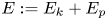 $E := E_k + E_p$:
 \begin{equation} \frac{\mathrm{d}E}{\mathrm{d}t} =-\epsilon_i - \epsilon_p + \mathcal{D}_u + \mathcal{D}_b. \end{equation}
Not only are the diffusive fluxes very weak, but they also have a tendency to cancel, thus to a very good approximation, the total change in the energy of the system is the energy lost to dissipation. Furthermore, once the inertial oscillations and perturbations have decayed to zero, we can equate the change in background potential energy and the energy lost to dissipation to the initial energy associated with the unbalanced motions. However, some of the simulations still have significant inertial energy after 20 inertial periods (figure 9). In order to assess the change in the potential energy of the balanced state, we must account for the oscillations in potential energy due to the differential horizontal advection by the inertial oscillations. Therefore, we define the potential energy of the balanced state to be the potential energy plus the cross kinetic energy:
 \begin{equation} E_{p,{b}} := E_p + E_{k,{c}}. \end{equation}
In doing so, we have made the assumptions that the buoyancy flux, geostrophic shear production and diffusive boundary fluxes are negligible. With these assumptions, the only active terms in the potential and cross kinetic energy equations are the geostrophic pressure work and horizontal differential advection through which kinetic and potential energy are exchanged. The cross kinetic energy oscillates about zero, hence the potential energy of the balanced state is the instantaneous potential energy plus the cross kinetic energy.
These assumptions are justified for almost all of our simulations as the diffusive fluxes are always weak and after 20 inertial periods the perturbation kinetic energy has decayed, assuming that the flow was unstable in the first place, to negligible values. Hence there is little scope for geostrophic shear production or buoyancy fluxes to transfer energy from the perturbation kinetic energy to the potential or cross kinetic energy (figure 9). The assumptions do not, at first sight, hold in the simulations with  ${{Ri}} = 1$,
  $\delta _0 = 0.75$ (SIM12 and SIM17), which have not reached their final state as the PSI modes grew slowly (table 1) and have significant perturbation (and inertial) kinetic energy. However, as we show shortly, when
  ${{Ri}} = 1$, the geostrophic shear production and buoyancy flux exactly cancel, and consequently the perturbations cannot exchange energy with the balanced state. Therefore, with this definition we find no change in the potential energy of the balanced state in these simulations (figure 15).

Figure 15. Fate of the initial inertial kinetic energy after 20 inertial periods for SIM01–13 (white backgrounds) and SIM16–18 (light grey backgrounds). We plot the terms of (5.7) as bar charts centred on the point in parameter space corresponding to the initial conditions of the simulation. The exceptions are SIM16–18, which have the same parameters as SIM11–13 and hence are positioned directly beneath. The bar chart  $y$-axes are normalised by the initial kinetic energy of the simulations. We indicate, by the grey blob, simulations in which the flow is stable to PSI.
Finally, defining the unbalanced energy as the total energy minus the geostrophic kinetic energy and balanced potential energy,  $E_{u} := E - E_{k,{g}} - E_{p,{b}}$, we can evaluate the change in the potential energy after 20 inertial periods,
 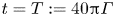 $t = T := 40{\rm \pi} \varGamma$, and determine the fate of the energy initially contained in the inertial oscillations:
 \begin{equation} E_{u}|_{t=0} = E_{u}|_{t=T} + \Delta E_{p,{b}} + \int_0^T \epsilon_{i}\,\mathrm{d}t + \int_0^T \epsilon_{p}\,\mathrm{d}t + \int_0^T \mathcal{D}_u\,\mathrm{d}t + \int_0^T \mathcal{D}_b\,\mathrm{d}t. \end{equation}
Note that with these definitions, the initial unbalanced energy is simply the inertial kinetic energy  $E_{k,{i}}|_{t=0}$ plus a negligible amount of perturbation kinetic energy due to the white noise. Similar to the plot of the kinetic energy budget (figure 9), we plot the terms on the right-hand side of this equation normalised by the initial unbalanced energy (figure 15).
We find that the potential energy of the system increases in all the cases with  ${{Ri}}^{-1} < 1$, which is consistent with our analysis of the kinetic energy in which the combined geostrophic shear production and buoyancy flux was found to be negative. The fraction of the initial unbalanced energy that goes into raising the potential energy of the balanced state increases as
  ${{Ri}}^{-1}$ gets smaller, although the dependence is weak for
  ${{Ri}}^{-1} < 3/4$. However, there exists a critical balanced Richardson number,
  ${{Ri}}_{c}(\delta )$, above which the flow is stable to PSI. For balanced Richardson numbers larger than the critical value, the inertial motions decay viscously and the balanced state is unchanged.
5.2. Potential vorticity
The modification of the balanced state requires a change in the PV that must occur via a boundary flux (Haynes & McIntyre Reference Haynes and McIntyre1987). Initially, the simulations start with uniform PV, 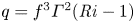 $q = f^3\varGamma ^2({{Ri}} - 1)$. For
  ${{Ri}} > 1$, while the baroclinic contribution
  $-f^3\varGamma ^2$ remains fixed, the mean stratification decreases, resulting in a decrease in the PV. We again draw a contrast with symmetric, and inertial, instabilities that occur when the PV is negative, and must increase the PV in order to reach stability. In the ocean and in many simulations, this is achieved by mixing with a reservoir of positive PV, such as the thermocline (Taylor & Ferrari Reference Taylor and Ferrari2009). However, in idealised simulations with uniform PV set-ups similar to ours, this can be achieved purely through boundary fluxes (Thorpe & Rotunno Reference Thorpe and Rotunno1989). In our case, however, there is no such requirement on the PV. PSI stabilises by damping its energy source, namely the inertial oscillations, and it is not obvious a priori that the PV will decrease. Indeed, if we start with larger
  ${{Ri}}$ such that the flow is stable to PSI, then there will be no change in the mean stratification, PV, or potential energy of the balanced state.
5.3.  ${{Ri}} = 1$

In our simulation set-up, the total buoyancy 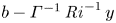 $b - \varGamma ^{-1}\,{{Ri}}^{-1}\,y$ and absolute momentum
  $u_g + u - \varGamma ^{-1}y$ satisfy the same equation, advection–diffusion with equal diffusivities (
 ${{Pr}} = 1$), and boundary conditions. When
  ${{Ri}} = 1$, they also have the same initial conditions, up to the inconsequential addition of white noise. Therefore, they evolve in the same way, and the PV, which is the Jacobian of the total buoyancy and absolute momentum, will remain zero. Furthermore,
  $u' = b'$, implying
  ${\langle u'w'\rangle } = {\langle b'w'\rangle }$, and we must have the exact cancellation of the geostrophic shear production and buoyancy flux (figures 8 and 9). As a result, there is no exchange of energy between the perturbations and the balanced state (figure 15). Finally, once the unbalanced motions die out, the vertical structure of the absolute momentum will be set by the fixed geostrophic shear, and the exact equality of the total buoyancy and absolute momentum means that the stratification of the balanced state is also fixed.
However, the unbalanced motions do not vanish totally. Although their energy content is very small, the remnant PSI modes can in some cases contribute significantly to the velocity and buoyancy gradients. The case with  ${{Ri}} = \delta _0 = 1$ is one such, and perhaps the most interesting as it corresponds to the ‘classic geostrophic adjustment problem’ of Tandon & Garrett (Reference Tandon and Garrett1994). After 20 inertial periods, the inertial oscillations have been almost completely damped out, but the PSI modes are prominent in plots of the shear and horizontal buoyancy gradient (figure 16). The PSI modes are still unstable to KH, and we see evidence of KH billows. Nonetheless, this simulation is very close to its final state. On scales larger than the KH billows, the PSI modes still contribute significantly to the horizontal buoyancy and vertical velocity gradients, and could therefore influence the future evolution of the front. It should be noted, however, that the PSI modes are not in geostrophic balance (figure 16c).

Figure 16. Sections of (a) the vertical derivative of the absolute momentum  $u_z + 1$, (b) the horizontal derivative of the total buoyancy
  $b_y - {{Ri}}^{-1}\,\varGamma ^{-1}$, and (c) the thermal wind imbalance
  $u_z + {{Ri}}\,\varGamma \,b_y$ from SIM18 after 20 inertial periods. Contours of total buoyancy are overlaid in black.
6. Conclusions
In this paper, we explored the 2-D stability of inertial shear at fronts to parametric subharmonic instability. We extended the linear stability analysis of T&T to include off-isopycnal modes, thus allowing for the buoyancy flux to play a role in the energetics, and non-hydrostatic perturbations, which arise in strong inertial shear. We find that both the critical value of the balanced Richardson number,  ${{Ri}}_{c}$, below which PSI occurs, and the growth rate of PSI, depend strongly on the strength of the inertial shear,
  $\delta$. While the growth rates in weak inertial shear are modest, growth rates in excess of
  $f/2$ are predicted for inertial shear that matches or exceeds the thermal wind shear. The optimal slope, in a coordinate system advected with the isopycnals, of the perturbations is a function of both
  ${{Ri}}$ and
  $\delta$. However, in strong inertial shear, an approximately along-isopycnal perturbation grows fastest.
We tested our linear stability analysis with a set of nonlinear 2-D simulations. We found discrepancies in the growth rates and perturbation slopes that can be attributed to viscous effects. Despite the viscous damping, growth rates of approximately  $f/3$ were obtained in some cases. The optimal perturbation slope was generally found to be shallower than predicted, and buoyancy fluxes played a small, but not insignificant, role in the energetics. However, the sign of the cumulative buoyancy flux was found to depend on
  ${{Ri}}$. The simulations also confirmed the prediction of the linear stability analysis that the geostrophic shear production would be negative. Unlike symmetric instability (SI) that primarily gains energy from the geostrophic shear, PSI draws energy out of the inertial oscillations, and some of that energy is put into the front. In the frontal zone set-up, this manifests itself as a differential horizontal advection that increases the potential energy of the front. However, for
  ${{Ri}}^{-1} \approx 1$, the buoyancy flux acts to extract potential energy out of the balanced front, counteracting this advection, and for
  ${{Ri}} = 1$, the two exactly balance and the potential energy of the balanced front is unchanged. This increase in potential energy is associated with a decrease in the stratification and potential vorticity (PV) of the balanced state. This unusual behaviour – most instabilities at fronts occur at the expense of the front's store of energy – occurs for only a small range of
  ${{Ri}}$; too large and PSI does not occur, too small and the front is unstable to SI. The increase in the potential energy of the balanced front is possible only because the front is initially unbalanced and hence there is an additional source of energy in the inertial motions.
Our numerical set-up, a 2-D frontal zone, places limitations on the dynamics that can occur and precludes some physical mechanisms that could influence the growth of PSI modes, secondary instabilities and the evolution of the balanced state. At a finite-width front, we would expect to find a closed overturning circulation that stands-up the front, increasing its potential energy. However, other processes may be at play, including the propagation of the near-inertial waves, frontogenesis and frontolysis, all of which could modify the development of PSI modes. Furthermore, the final balanced state and its potential energy are dependent on the turbulent mixing of buoyancy induced by the secondary instabilities. However, the use of hyper-viscosity and the restriction to two dimensions modifies the evolution of the secondary instabilities (Staquet Reference Staquet2000) and consequently limits the ability of our simulations to represent mixing realistically.
Finally, we comment on physical scenarios where PSI might be important. The first is geostrophic adjustment, where PSI could rapidly damp the transient motions. However, it is thought that on longer time scales, the majority of the adjustment and restratification of the ocean mixed layer is as a result of mixed-layer instabilities (MLIs) (Boccaletti et al. Reference Boccaletti, Ferrari and Fox-Kemper2007; Fox-Kemper et al. Reference Fox-Kemper, Ferrari and Hallberg2008). While the growth rates of PSI in strong inertial shear exceed those of MLI,  $\sigma _{MLI}^2 = (5/54)(1+{{Ri}})^{-1}f^2$ (Stone Reference Stone1970), the two are comparable as the inertial shear decays. Furthermore, the generation of PV at the boundary, and subsequent advection into the interior of the front by PSI modes, can create PV gradients potentially contributing to a baroclinic or barotropic instability. The potential coexistence and interplay between PSI and MLI is a very interesting but inherently three-dimensional problem, and is left to a future study. Geostrophic adjustment generally occurs after a very intense forcing event, such as a storm. However, we do not necessarily require such dramatic events to trigger PSI. The PSI mechanism requires two things: first, a front with a low balanced Richardson number, and second, inertial shear. Fronts preconditioned for PSI, in the sense that they have low balanced Richardson numbers, can be found in regions with lateral buoyancy gradients, a shallow convective or frictional surface boundary layer, and a deeper pycnocline. The weakly stratified region between the boundary layer and pycnocline often persists in or near a state of marginal stability to SI, that is,
  ${{Ri}} = 1$. It is well documented that down-front winds will force SI in this scenario (Thomas et al. Reference Thomas, Taylor, Ferrari and Joyce2013). However, there is also the possibility that ‘stabilising’ winds will force strong inertial oscillations that then undergo parametric subharmonic instability.
Acknowledgements
Some of the computing for this project was performed on the Sherlock cluster. We would like to thank Stanford University and the Stanford Research Computing Center for providing computational resources and support that contributed to these research results.
Funding
J.P.H. and L.N.T. were supported by a grant from the National Science Foundation, SUNRISE, award no. OCE-1851450. L.N.T. was additionally supported by Office of Naval Research grant N00014-18-1-2798.
Declaration of interests
The authors report no conflict of interest.
Appendix A. Numerical procedure to find eigenvalues and eigenfunctions
We use a fourth-order Runge–Kutta scheme to integrate (2.14) from two linear independent initial conditions for one period. We can express these two solutions, denoted by subscripts  $a$ and
  $b$, as
 \begin{equation} \begin{bmatrix}\varPsi_a(t) & \zeta_a(t) \\ \varPsi_b(t) & \zeta_b(t)\end{bmatrix} = \boldsymbol{\mathsf{A}}\begin{bmatrix} \mathrm{e}^{\mu t} & 0 \\ 0 & \mathrm{e}^{-\mu t} \end{bmatrix}\begin{bmatrix}\varPsi_1(t) & \zeta_1(t) \\ \varPsi_2(t) & \zeta_2(t)\end{bmatrix}. \end{equation}
Our aim is to find  $\mu$ and invert
  $\boldsymbol{\mathsf{A}}$ to get the eigenfunctions. Let
 \begin{equation} \boldsymbol{\mathsf{S}}(t) =\begin{bmatrix}\varPsi_a(t) & \zeta_a(t) \\ \varPsi_b(t) & \zeta_b(t)\end{bmatrix}, \quad \boldsymbol{\mathsf{D}}(t) = \begin{bmatrix} \mathrm{e}^{\mu t} & 0 \\ 0 & \mathrm{e}^{-\mu t} \end{bmatrix}, \quad \boldsymbol{\mathsf{M}}(t) = \begin{bmatrix}\varPsi_1(t) & \zeta_1(t) \\ \varPsi_2(t) & \zeta_2(t)\end{bmatrix}. \end{equation}
At  $t=0$, we have
  $\boldsymbol{\mathsf{D}} = \boldsymbol{\mathsf{I}}$ and we choose
  $\boldsymbol{\mathsf{S}}(0) = \boldsymbol{\mathsf{I}}$. We therefore have
  $\boldsymbol{\mathsf{A}} = \boldsymbol{\mathsf{M}}(0)^{-1}$. Integrating forward in time to
  $t = T = 2{\rm \pi}$, and using the periodicity of
  $\boldsymbol{\mathsf{M}}$, we have
 \begin{equation} \boldsymbol{\mathsf{S}}(T) = \boldsymbol{\mathsf{A}}\,\boldsymbol{\mathsf{D}}(T)\,\boldsymbol{\mathsf{A}}^{-1}, \end{equation}
which is precisely the diagonalisation of  $\boldsymbol{\mathsf{S}}(T)$, and immediately gives us not only
  $\mu$ from the eigenvalues of
  $\boldsymbol{\mathsf{S}}(T)$, but also the columns of
  $\boldsymbol{\mathsf{A}}$ as the right eigenvectors of
  $\boldsymbol{\mathsf{S}}(T)$. Furthermore, to calculate
  $\mu$, we do not need to save
  $\boldsymbol{\mathsf{S}}(t)$, and we validate our integration by checking that the determinant of
  $\boldsymbol{\mathsf{S}}(T)$ is
  $1 = \mathrm {e}^{\mu T}\mathrm {e}^{-\mu T}$.
The viscous solutions are found similarly, but as the equations are no longer time-reversible, we do not have the property that the determinant of  $\boldsymbol{\mathsf{S}}(T)$ is 1.
Appendix B. Simulation energetics
We construct the evolution equations for the domain-averaged (denoted  $\langle {\cdot }\rangle$) energetics. DIABLO solves (3.1) for the ageostrophic component of the flow. From this, we derive evolution equations for the perturbation kinetic energy
  $E_{k,{p}} = \tfrac {1}{2}\left \langle \boldsymbol {u}'\boldsymbol {\cdot } \boldsymbol {u}'\right \rangle$, and inertial kinetic energy
  $E_{k,{i}} = \tfrac {1}{2}\left \langle \overline{\boldsymbol{u}}\boldsymbol {\cdot } \overline{\boldsymbol{u}}\right \rangle$. Taking the dot product of
  $\boldsymbol {u}$ with (3.1a) and taking the domain average gives
 \begin{equation} \frac{\mathrm{d}}{\mathrm{d}t}\left(\frac{1}{2}\left\langle \boldsymbol{u}\boldsymbol{\cdot} \boldsymbol{u}\right\rangle\right) + \left\langle uw\right\rangle -{{Ri}}\left\langle wb\right\rangle =-\frac{{{Ek}}}{\varGamma}\left\langle \frac{\partial\boldsymbol{u}}{\partial z}\boldsymbol{\cdot}\frac{\partial\boldsymbol{u}}{\partial z} + \nu_H\,\frac{\partial^2 \boldsymbol{u}}{\partial y^2}\boldsymbol{\cdot}\frac{\partial^2 \boldsymbol{u}}{\partial y^2}\right\rangle, \end{equation}
where the advective and pressure works terms vanish due to the boundary conditions, the Coriolis terms vanish identically, and the viscous terms have been written in negative definite form with vanishing boundary terms. Splitting terms into lateral mean and perturbation parts, we have
 \begin{align} &\frac{\mathrm{d}}{\mathrm{d}t}\Bigl(\underbrace{\frac{1}{2}\left\langle \overline{\boldsymbol{u}}\boldsymbol{\cdot} \overline{\boldsymbol{u}}\right\rangle}_{E_{k,{i}}} + \underbrace{\frac{1}{2}\left\langle \boldsymbol{u}'\boldsymbol{\cdot} \boldsymbol{u}'\right\rangle}_{E_{k,{p}}}\Bigr) + \underbrace{\left\langle u'w'\right\rangle}_{-\mathcal{P}_{g}} -\underbrace{{{Ri}}\left\langle w'b'\right\rangle}_\mathcal{B}\nonumber\\ &\quad =-\underbrace{\frac{{{Ek}}}{\varGamma}\left\langle \frac{\partial\overline{\boldsymbol{u}}}{\partial z}\boldsymbol{\cdot}\frac{\partial\overline{\boldsymbol{u}}}{\partial z}\right\rangle}_{\epsilon_{i}} -\underbrace{\frac{{{Ek}}}{\varGamma}\left\langle \frac{\partial\boldsymbol{u}'}{\partial z}\boldsymbol{\cdot}\frac{\partial\boldsymbol{u}'}{\partial z} + \nu_H\,\frac{\partial^2 \boldsymbol{u}'}{\partial y^2}\boldsymbol{\cdot}\frac{\partial^2 \boldsymbol{u}'}{\partial y^2}\right\rangle}_{\epsilon_{p}}. \end{align}
Taking the lateral mean of the momentum equation (3.1a), and noting that the vertical momentum equation reduces to hydrostatic balance, we have
 \begin{equation} \frac{\mathrm{d}\overline{\boldsymbol{u}}}{\mathrm{d}t} + \frac{\partial }{\partial z}\overline{\boldsymbol{u}'w'} + \frac{1}{\varGamma}\,\hat{\boldsymbol{z}}\boldsymbol{\wedge} \overline{\boldsymbol{u}} = \frac{{{Ek}}}{\varGamma}\,\frac{\partial^2\overline{\boldsymbol{u}}}{\partial z^2}. \end{equation}
We construct the evolution equation for the inertial kinetic energy (3.8b) by taking the dot product with  $\overline{\boldsymbol{u}}$, taking the domain average, and utilising the boundary conditions to shift derivatives:
 \begin{equation} \frac{\mathrm{d}}{\mathrm{d}t}\Bigl(\underbrace{\frac{1}{2}\left\langle \overline{\boldsymbol{u}}\boldsymbol{\cdot}\overline{\boldsymbol{u}}\right\rangle}_{E_{k,{i}}}\Bigr) \underbrace{{}-\frac{\partial\overline{\boldsymbol{u}}}{\partial z}\,\overline{u'w'}}_{\mathcal{P}_{a}} =-\underbrace{\frac{{{Ek}}}{\varGamma}\left\langle \frac{\partial\overline{\boldsymbol{u}}}{\partial z}\boldsymbol{\cdot}\frac{\partial\overline{\boldsymbol{u}}}{\partial z}\right\rangle}_{\epsilon_{i}}. \end{equation}
We get the evolution equation for the perturbation kinetic energy (3.8a) by subtracting (B3) from (B1b).
From (B2), we construct the evolution equation for the cross kinetic energy by taking the dot product with the geostrophic momentum  $\boldsymbol {u}_g = z\hat {\boldsymbol {x}}$, and taking the domain average:
 \begin{equation} \frac{\mathrm{d}}{\mathrm{d}t}\left(\underbrace{\left\langle \boldsymbol{u}_g\boldsymbol{\cdot}\overline{\boldsymbol{u}}\right\rangle}_{E_{k,{c}}}\right) + \underbrace{\left\langle u'w'\right\rangle}_{\mathcal{P}_{g}} - \frac{1}{\varGamma}\left\langle \overline{v}z\right\rangle \underbrace{{}-\frac{{{Ek}}}{\varGamma}\,\overline{u}|^{z=1}_{z=-1}}_{\mathcal{D}_u}, \end{equation}
where we have used integration by parts to shift the derivative from the eddy momentum flux onto the geostrophic velocity, and reduced the viscous terms to a boundary flux. We have a term arising from the Coriolis force. However, using the geostrophic balance, we can reinterpret this as the work done against the geostrophic pressure gradient,  $\varPi _y$, by the inertial oscillations:
 \begin{equation} \frac{1}{\varGamma}\,u_g =-\varPi_y \implies \frac{1}{\varGamma}\,z =-\varPi_y \implies \frac{1}{\varGamma}\left\langle \overline{v}z\right\rangle = \underbrace{-\left\langle \overline{v}\varPi_y\right\rangle}_{\mathcal{P}_{p}}. \end{equation}
 The potential energy,  $E_{p} := {\langle -{{Ri}}\,bz\rangle }$, evolution equation is formed by multiplying (3.1b) with
  $-{{Ri}}\,z$ and taking the domain average:
 \begin{equation} \frac{\mathrm{d}E_p}{\mathrm{d}t} =-\underbrace{{{Ri}}\left\langle w'b'\right\rangle}_\mathcal{B} \underbrace{{}-\frac{1}{\varGamma}\left\langle \overline{v}z\right\rangle}_{\mathcal{B}_{H}} + \underbrace{\frac{{{Ek}}}{\varGamma}\left[\overline{b} - z\right]^{z=1}_{z=-1}}_{\mathcal{D}_b}, \end{equation}
where we again use integration by parts to extract the buoyancy flux and reduce the viscous term down to a boundary flux. We can interpret the differential advection of horizontal buoyancy,  $\mathcal {B}_{H}$, as the advection of potential energy and the buoyancy flux associated with the background buoyancy gradient:
 \begin{align} -\frac{1}{\varGamma}\left\langle \overline{v}z\right\rangle &= \left\langle \frac{\partial}{\partial y}\left(\overline{v}\,{{Ri}}\left[-\frac{1}{\varGamma\,{{Ri}}}\,y\right]z\right)\right\rangle\nonumber\\ &= \left\langle \frac{\partial}{\partial y}\left(v\,{{Ri}}\left[-\frac{1}{\varGamma\,{{Ri}}}\,y\right]z\right)\right\rangle - \left\langle \frac{\partial}{\partial y}\left(v'{{Ri}}\left[-\frac{1}{\varGamma\,{{Ri}}}\,y\right]z\right)\right\rangle\nonumber\\ &= \left\langle \frac{\partial}{\partial y}\left(v\,{{Ri}}\left[-\frac{1}{\varGamma\,{{Ri}}}\,y\right]z\right)\right\rangle - \left\langle \left(\frac{\partial v'}{\partial y}\right){{Ri}}\left[-\frac{1}{\varGamma\,{{Ri}}}\,y\right]z\right\rangle\nonumber\\ &= \left\langle \frac{\partial}{\partial y}\left(v\,{{Ri}}\left[-\frac{1}{\varGamma\,{{Ri}}}\,y\right]z\right)\right\rangle + \left\langle \left(\frac{\partial w}{\partial z}\right){{Ri}}\left[-\frac{1}{\varGamma\,{{Ri}}}\,y\right]z\right\rangle\nonumber\\ &=-\left\langle \frac{\partial}{\partial y}\left(-v\,{{Ri}}\left[-\frac{1}{\varGamma\,{{Ri}}}\,y\right]z\right)\right\rangle - \left\langle \frac{\partial }{\partial z}\left(-w\,{{Ri}}\left[-\frac{1}{\varGamma\,{{Ri}}}\,y\right]z\right)\right\rangle - {{Ri}}\left\langle w\left[-\frac{1}{\varGamma\,{{Ri}}}\,y\right]\right\rangle. \end{align}
Note that this entire manipulation is invariant under translations in  $y$.
$y$.


 Open access