


1. Introduction
Turbulent flows over rough surfaces play an integral role in many industrial applications, as well as atmospheric flows over natural and non-natural terrains. Significant economic and performance benefits can arise from a better understanding of the connection between roughness geometry, boundary layer flow structure and the resulting drag. For this reason, effects of surface roughness on the dynamics of boundary layers have been under investigation for many years (Raupach, Antonia & Rajagopalan Reference Raupach, Antonia and Rajagopalan1991; Jiménez Reference Jiménez2004; Castro Reference Castro2007).
Rough surfaces modulate the flow locally in the roughness sublayer. One way of quantifying these modulations is by analysis of dispersive stresses, the spatial variations which develop in the mean flow field when compared to the horizontally averaged mean flow. These dispersive stresses are in addition to the Reynolds stresses near the wall but diminish in magnitude as a function of wall-normal distance, and the Reynolds stresses dominate in the outer layer. Therefore, for homogeneous roughness, effects of the rough wall are confined to the sublayer, and the outer layer can become independent of the details of the roughness, referred to as outer-layer similarity (Townsend Reference Townsend1980).
At sufficiently high Reynolds numbers and greater separation of scales, outer-layer similarity has been observed wherein the velocity profile shows trends consistent with the standard log-wake function (Bandyopadhyay & Watson Reference Bandyopadhyay and Watson1988; Volino, Schultz & Flack Reference Volino, Schultz and Flack2007). This similarity can be present for fully rough boundary layers on the condition that the length scale of the rough wall is small compared to the boundary layer height (Perry & Abell Reference Perry and Abell1977). In contrast it has been observed, in certain circumstances, that the rough wall can in fact affect the velocity in the outer layer (Shafi & Antonia Reference Shafi and Antonia1997; Placidi & Ganapathisubramani Reference Placidi and Ganapathisubramani2018).
In addition to the separation of scales between the boundary layer height and the roughness length, spatial heterogeneity is also an important consideration for how the surface affects the outer layer flow. Once spanwise heterogeneity of the roughness is introduced, it has been noted that collapsing outer layer dynamics no longer hold and secondary motions can cover the entire boundary layer height (Wang & Cheng Reference Wang and Cheng2005; Barros & Christensen Reference Barros and Christensen2014; Willingham et al. Reference Willingham, Anderson, Christensen and Barros2014; Anderson et al. Reference Anderson, Barros, Christensen and Awasthi2015; Vanderwel & Ganapathisubramani Reference Vanderwel and Ganapathisubramani2015; Meyers, Ganapathisubramani & Cal Reference Meyers, Ganapathisubramani and Cal2019). Furthermore, the decay of dispersive stresses for such streamwise roughness elements has been found to scale with the spanwise spacing (Chan et al. Reference Chan, MacDonald, Chung, Hutchins and Ooi2018; Yang & Anderson Reference Yang and Anderson2018). Reynolds et al. (Reference Reynolds, Hayden, Castro and Robins2007) observed secondary flows form over repeating arrays of cubes in a wind tunnel. Barros & Christensen (Reference Barros and Christensen2014) observed low- and high-momentum pathways occupied by large secondary swirling motions in the mean flow over the irregular surface topology of a replica of a damaged turbine blade. A systematic study of three-dimensional roughness effects on secondary motion in simulated pipe flow was recently presented by Chan et al. (Reference Chan, MacDonald, Chung, Hutchins and Ooi2018). The study varied the roughness height and wavelength to classify the subsequent developing secondary motion, finding that coherent stress scales with wavelength and height. The arrangement of the elements is also an important factor in stress contribution near the surface of the roughness (Orlandi & Leonardi Reference Orlandi and Leonardi2006). Coceal et al. (Reference Coceal, Thomas, Castro and Belcher2006) investigated cubes in an aligned and staggered formation, noting that the staggered array showed nearly negligible dispersive stresses above the roughness, in contrast to those formed above the aligned cubes.
Numerous studies have investigated how the rough wall geometries interact with the developing boundary layer, but these geometries are often single-scale elements. Recently, experimental and numerical studies have begun quantifying these topological length scales and their effects (Mejia-Alvarez & Christensen Reference Mejia-Alvarez and Christensen2013; Yang & Meneveau Reference Yang and Meneveau2017; Medjnoun et al. Reference Medjnoun, Rodriguez-Lopez, Ferreira, Griffiths, Meyers and Ganapathisubramani2021). The work of Medjnoun et al. (Reference Medjnoun, Rodriguez-Lopez, Ferreira, Griffiths, Meyers and Ganapathisubramani2021) provides one of the first systematic experimental campaigns to characterize the dynamics above multi-scale fractal roughness elements. The study used four roughness elements, with varying scales included, to quantify the effects of scale hierarchy. Results show that the intermediate scale of the roughness scale hierarchy contributes the greatest amount to overall drag. This study also found that the presence of large-scale motion, a consequence of the spacing between the largest cuboids, impacted the canopy region and outer flow, and therefore a lack of outer-layer similarity was reported.
With greater relevance to real world applications, the implications of characterizing the dependence of developing secondary motions and drag on the individual scales included on the roughness element are profound. Utilizing the same roughness elements as those presented in the work of Medjnoun et al. (Reference Medjnoun, Rodriguez-Lopez, Ferreira, Griffiths, Meyers and Ganapathisubramani2021), i.e. the same fractal dimensions of the cuboids included in the rough-wall geometry, experiments are performed to quantify the formation of secondary motions over rough walls comprising elements with varying levels of scales in a staggered arrangement. The staggered formation of the roughness peaks causes the typical channels of flow which are observed in Medjnoun et al. (Reference Medjnoun, Rodriguez-Lopez, Ferreira, Griffiths, Meyers and Ganapathisubramani2021) to disperse. Therefore this study seeks to describe the effect of heterogeneity on the flow structure above the roughness elements and quantify the decay of dispersive stresses with wall-normal distance.
2. Experimental methods
Experiments were conducted in the closed-loop wind tunnel located at Portland State University with a working section of  $0.8\ {\rm m} \times 1.2\ {\rm m}$ in the cross-plane and 5 m in length (Ali et al. Reference Ali, Bossuyt, Viggiano, Ganapathisubramani, Meyers and Cal2019). A schematic representation of the experiment is provided in figure 1(a) along with the measurement coordinate system. The slightly diverging cross-section ensures a nominally zero-pressure gradient for the free-stream (inlet) velocity of $U_{\infty }=5\ {\rm m}\ {\rm s}^{-1}$.

Figure 1. (a) Schematic of the closed-circuit wind tunnel (not to scale). (b) Spatial representation of the nine PIV planes and their location within the staggered element formation. (c) Spatial layout of R-123, R-12 and R-13.
The rough surface consisted of fractal elements, mounted on an acrylic sheet and placed directly on the wind tunnel floor. The fractal elements have a width,  $W$, of 100 mm and a height, $H$, which ranges from 8.5 to 10.5 cm depending on the number of fractal scales included. The elements span the floor of the entire test section in a staggered arrangement; see figure 1(b). The dynamics of flow above three different roughness elements are investigated, wherein three scales of fractal dimensions are included, with large-scale cuboids containing smaller cuboids. There are three levels of scales that decrease in size with a power law as the number of the occurrences of the element increases with a power law. Herein, the three tiles will be denoted by R-123, R-12 and R-13 (referring to the inclusion of the largest scale, 1, the intermediate scale, 2, and the smallest scale, 3) as shown in figure 1(c). A detailed description of the methodology of the multi-scale elements can be found in Medjnoun et al. (Reference Medjnoun, Rodriguez-Lopez, Ferreira, Griffiths, Meyers and Ganapathisubramani2021) (see also the study of Zhu & Anderson (Reference Zhu and Anderson2018) for the iteration function description). In total, the wind tunnel floor was covered with 46 rows of roughness elements. The boundary layer was naturally developed, starting from a uniform inflow at inlet; i.e. no turbulence grid was used. The measurement planes spanned rows 34 to 36, 3.5 m downstream from the tunnel entrance.
The stereoscopic particle image velocimetry (S-PIV) set-up consisted of two 4 megapixel CCD cameras and a Litron Nano double-pulsed Nd:YAG laser. The camera lenses had a focal length of 100 mm and a fixed aperture of  $f2.8$. The images were processed in Davis 8.0 using multi-grid stereo cross-correlation with one pass with an interrogation area of $48 \times 48$ pixels and 50 % overlap followed by two passes with an interrogation size of $24 \times 24$ pixels. This results in a resolution of 0.9–1 mm for all generations. The uncertainty of the velocity in the streamwise and wall-normal directions was ${\pm }0.08$ ( ${\rm m}\ {\rm s}^{-1}$) and ${\pm }0.01$ ( ${\rm m}\ {\rm s}^{-1}$) respectively. Diethylhexyl sebacate was used to seed the wind tunnel and was aerosolized by a seeding generator, with a constant density throughout the experiment. Given $x$,
$x$,  $y$ and $z$ as the streamwise, wall-normal and spanwise coordinates, S-PIV planes were taken in the $yz$ domain at nine streamwise locations. A schematic of the arranged elements with the corresponding $yz$ planes is shown in figure 1(b). The gradient of colour used here is replicated when results are presented by normalized plane with $x/W=[0:0.125:1]$. For each measurement plane, 4000 snapshots were acquired to achieve second-order statistical convergence. A subset of snapshots of the instantaneous streamwise velocity are provided as a supplementary movie available at https://doi.org/10.1017/jfm.2022.262.
Key quantities of the boundary layer flow are presented in table 1. The boundary layer height,  $\delta$, is defined by 99 % of the free-stream velocity, $U_{\infty }$, with a datum at the top of the acrylic sheet for all generations. The shear stress at the wall $\tau _{w}$ was computed based on the integrated boundary layer equation and the friction velocity $u_*=(\tau _{w}/\rho )^{1/2}$ (Brzek et al. Reference Brzek, Cal, Johansson and Castillo2007). There is a significant increase in skin friction due to roughness, specifically as a result of including the intermediate and large scales. As shown, R-123 and R-12 induce higher drag in comparison with the third generation, R-13. Dependent on scales of roughness, the near-wall physics is significantly altered by the viscous stress contribution. Trends similar to those observed in the skin friction coefficient, $C_f$, occur for the momentum thickness $\theta$ and the associated Reynolds number, as well as for the friction velocity $u_*$: these again present comparable values between the R-123 and R-12 elements while exhibiting a decrease in magnitude for R-13. Other relevant parameters from the table are discussed with respect to inner and outer scaling arguments in the following section.
Table 1. Aerodynamic flow parameters for each roughness type.

3. Results
3.1. Parameter evaluation
Distributions of the temporally and spatially (double) averaged velocity  $\langle \bar {u} \rangle _{xz}$ normalized by the friction velocity are shown in figure 2(a). It is of note that the friction velocity for a given roughness element generation has minimal differences from plane to plane, with a maximum standard deviation over the nine $yz$ planes of $0.0016\ {\rm m}\ {\rm s}^{-1}$. For the entirety of the article, $\langle \cdot \rangle$ signifies spatial averaging with respect to the direction specified in the included subscript, and the overline denotes temporal averaging. The curves are presented in terms of $(y-d)/y_0$, where $d$ is the zero-plane displacement and $y_0$ is the roughness height. The inset is included to show $\langle \bar {u}^+ \rangle _{xz}$ as a function of inner scaling of the wall-normal location, $y^+-d^+=(y-d)u_*/\nu$. The three roughness element statistics are compared against the log-law $\langle \bar {u}^+ \rangle _{xz} \equiv \langle \bar {u} \rangle _{xz}/u_* = (1/\kappa )\ln ((y-d)/y_0)$, where the von Kármán constant is $\kappa =0.4$. The roughness height $y_0$ is obtained from the log-law and is given in table 1. The trend follows that of the drag coefficient, showing comparable values for R-123 and R-12, followed by a sharp decrease in magnitude for R-13.

Figure 2. (a) Averaged velocity profiles in inner variables and (b) velocity-defect profiles for the three generations, the Iter $_{123}$ curve of Medjnoun et al. (Reference Medjnoun, Rodriguez-Lopez, Ferreira, Griffiths, Meyers and Ganapathisubramani2021) and smooth wall direct numerical simulation data of (Sillero et al. Reference Sillero, Jiménez and Moser2013). Inset: the velocity-defect in semilog axes.
An alternative expression for the mean streamwise velocity,
 \begin{equation} \langle \bar{u}^+ \rangle_{xz} = \frac{1}{\kappa}\ln(y^+{-}d^+)+B-\Delta U^+, \end{equation}
gives rise to the roughness function  $\Delta U^+$. Here the constant $B$ is given a priori as 5.1. Again, $d$ is the shift in the wall-normal plane due to roughness, and calculated values are provided in table 1. This parameter is the value that minimizes the differences between the right- and left-hand sides of the derivative (with respect to $y$) of (3.1), also termed the indicator function, and defined as $(y^+-d^+)\,{\rm d} \langle \bar {u}^+ \rangle _{xz} /{\rm d}y^+=1/\kappa$, where $\kappa$ is assumed to be universal (Medjnoun et al. Reference Medjnoun, Rodriguez-Lopez, Ferreira, Griffiths, Meyers and Ganapathisubramani2021). Note that $d=0$ for a smooth wall.
The velocity shift,  $\Delta U^+$, is another roughness-related quantity, providing the change in momentum due to the rough surface; it is determined based on differences in the normalized velocity curves for the inner layer. Specifically, once $d$ is determined, $\Delta U^+$ is chosen to equate $\varPsi = \langle \bar {u}^+ \rangle _{xz} - (1/\kappa )\ln (y^+-d^+)-B+\Delta U^+$ to zero, also indicating the inertial sublayer. Experimentally determined $\Delta U^+$ values are included in table 1 for the three elements. Previous tendencies observed are substantiated and a momentum loss is observed that monotonically decreases from R-12 to R-123 to R-13. Minimal difference is observed between the two flows that contain the intermediate scales, while the R-13 presents a large decrease in comparison. The outer-region flow is often described by the velocity-defect law, the difference between free-stream velocity $U_{\infty }$ and the mean velocity profile $\langle \bar {u} \rangle _{xz}$:
 \begin{equation} \frac{U_{\infty}-\langle \bar{u}\rangle_{xz}}{u_*} ={-}\frac{1}{\kappa}\log\left(\frac{y-d}{\delta}\right)+\frac{\varPi}{\kappa} \left[2-w\left(\frac{y-d}{\delta}\right)\right]. \end{equation}
Included in this description are the universal wake function  $w$ and the wake strength parameter $\varPi$, which is said to be 0.55 for smooth walls (Coles Reference Coles1956). The resulting velocity-defect curve, with parameters based on the roughness element R-123, is presented in figure 2(b) along with the experimental profiles of the normalized defect. Furthermore, for comparison, the figure includes the aligned experimental data, Iter $_{123}$, of Medjnoun et al. (Reference Medjnoun, Rodriguez-Lopez, Ferreira, Griffiths, Meyers and Ganapathisubramani2021), as they correspond to the same roughness element as R-123, arranged with aligned peaks. It also includes smooth-wall data from direct numerical simulation (Sillero, Jiménez & Moser Reference Sillero, Jiménez and Moser2013). The inset provides a semilogarithmic representation of the curves to show the dependence on $y$ in the near-wall region. Here, a hierarchy is formed. Closest to the wall, the largest deficit in velocity occurs over the R-12 elements, while R-13 shows the least near-wall effects on the velocity. This relationship is dampened as the $y$ location increases. Notable differences are observed for the data from the aligned formation, Iter $_{123}$. The curves deviate as the flow approaches the wall, near $y/\delta$ of 0.6, indicating that the aligned element arrangement leads to a greater effect on the inner and outer layers. Small deviations occur, but a near collapse is observed between the staggered roughness and the smooth-wall curve of the velocity deficit. The inset allows the observation of the log-law, which occurs farther from the wall for the aligned data than for the staggered. This is also noted in the article of Medjnoun et al. (Reference Medjnoun, Rodriguez-Lopez, Ferreira, Griffiths, Meyers and Ganapathisubramani2021), which found the inertial sublayer to be 0.2 $\delta$–0.3 $\delta$, while this study finds that the inertial sublayer does not exceed 0.13 $\delta$, a location more typically observed in a smooth-wall boundary layer. Finally, there are notable differences between the wake parameters in the aligned cases of Medjnoun et al. (Reference Medjnoun, Rodriguez-Lopez, Ferreira, Griffiths, Meyers and Ganapathisubramani2021) and the staggered arrangement presented here. For a given boundary layer, the wake parameter can be found through fitting of composite equations, and resulting values for the present study are provided in table 1. The wake strength parameters of aligned elements range from $\varPi =0.17\text {--}0.25$, while the staggered formation presents values of 0.54–0.58, which agree more closely with those obtained for smooth walls; recall that $\varPi =0.55$ according to Coles (Reference Coles1956). Note that both studies find the element with the intermediate and large scales, R-12, to have the largest wake strength.
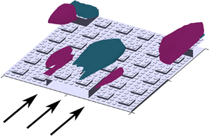
Iso-surfaces of the time-averaged wall-normal velocity are shown as an inset of figure 3 for each generation (arrows indicate flow direction). Dependence of the wall-normal velocity on the locations within the measurement volume is seen in each generation. This is indicated by the deficit of vertical velocity along the centre of the measurement plane, represented by the red iso-surface. This is due to the peak of the element at the front of the element. The velocity recovers as the flow along the edges of the interrogation window approaches the two peaks of the staggered formation, visible from the two blue surfaces forming at  $x/W\simeq 0.75$.

Figure 3. Wall-normal velocity, averaged over the spanwise locations  $\langle \bar {v}\rangle _z/u_*$, for each plane and generation. Inset: iso-surfaces of $\bar {v}/u_*$. Positive (negative) structures are blue (red), with a threshold of $\pm$0.3 for the representation.
The magnitude and extent of the vertical velocity vary for the three multi-scale elements; they are presented in figure 3 for all planes considered for each roughness element type. The characteristic height of the largest scale of the roughness (dashed line) is included in this and subsequent figures to better show attenuations due to the topography. This provides quantitative information on the location and magnitude of the formed structures observed in the iso-surfaces. First, the large deficit occurring directly after the peak (planes  $x/W=0.25$ to $x/W=0.5$) reaches nearly $-0.5$ for all generations, and is followed immediately by a shift to positive vertical velocity at the spanwise edges of the measurement volume ( $x/W=0.75$ and $x/W=0.875$). All three roughness elements present similar trends with respect to location, although the magnitude is increased in the flows over R-123 and R-12 in comparison to R-13.
3.2. Secondary motion
In relation to the formation of motion across the elements, momentum conservation becomes of interest. Through a horizontal spatial averaging scheme, the momentum equation can be expressed to yield the spatial correlations of the mean field, including the dispersive stress (Raupach & Shaw Reference Raupach and Shaw1982). To study the spatial dependence of dispersive stress contributions and characterize spatial inhomogeneity of the momentum balance near the roughness, one can examine the product of dispersive fluctuations in comparison to an average in  $x,z$ (Vanderwel et al. Reference Vanderwel, Stroh, Kriegseis, Frohnapfel and Ganapathisubramani2019) as defined by $\overline {u_{i}}^{\prime \prime } \overline {u_{j}}^{\prime \prime } = (\bar {u}_{i} -\langle \bar {u}_{i}\rangle _{xz}) (\bar {u}_{j} -\langle \bar {u}_{j}\rangle _{xz})$. Here the double prime denotes the product of fluctuations relative to the spatial average.
The iso-surfaces of the Reynolds shear stress for the given three generations are presented inset in figure 4. Only negative (red) structures form along the centre and edges of the interrogation volume for R-123, R-12 and R-13. The thresholding is chosen to provide near-wall structures while mitigating noise within representation. Again, the structures appear following a peak of the elements and disappear directly prior to the following peak. The main figure presents  $\langle \overline {u^{\prime }v^{\prime }}\rangle _z$ as a function of the normalized wall-normal location. For each fractal generation, all streamwise locations are presented ( $x/W=0$ to $x/W=1$) to show effects due to position. At first glance, all curves are oriented in a similar manner and average to similar values. Large differences are observed from plane to plane for generations R-123 and R-12 at the nearest wall locations. There exists a cyclical dependence of the magnitude on the location. Specifically, the smallest stresses are observed at planes $x/W=0$, $x/W=0.125$ and $x/W=1$. Furthermore, there exists a buildup of stress as the downstream location increases, with the largest values at $x/W=0.75$ for all generations. This location sits directly prior to the onset of peaks (along the outside) and valleys (at the centre), which occur at the end of the measurement volume (at $x/W=1$). This cyclical behaviour is most easily seen in the roughness elements R-123 and R-12. Although present, the dependence on streamwise location is much less pronounced for R-13 owing to the exclusion of the intermediate-scale cuboids, with which a greater amount of drag is associated. Note that the alternating of the structures observed in the iso-surface representation is not visible when the stress is spatially averaged; therefore minimal differences are observed from plane to plane for $\langle \overline {u^{\prime }v^{\prime }}\rangle _z$.

Figure 4. Figure shows  $\langle \overline {u^{\prime }v^{\prime }}\rangle _{z} /u_*^2$ for all planes. Inset: iso-surface of stress for each element, $\text {threshold}=-1$. All structures are negative.
Dispersive stresses become an important parameter in momentum flux when the rough wall becomes spatially inhomogeneous. To illustrate visually the stresses that arise from the peaks and valleys of the elemental array, the iso-surface of the dispersive shear stress,  $\bar {u}^{\prime \prime }\bar {v}^{\prime \prime }/u_*^2$, is included in figure 5 (inset). Each generation presents stresses which equate to upwash/downwash motions which interact with the streamwise momentum. In contrast to the aligned case of Medjnoun et al. (Reference Medjnoun, Rodriguez-Lopez, Ferreira, Griffiths, Meyers and Ganapathisubramani2021), there is no clear path that can be continuously taken by the momentum, and a disruption of the momentum flux is observed for all generations of elements owing to the staggered formation of the rough wall, mirroring trends observed for staggered cube roughness (Coceal et al. Reference Coceal, Thomas, Castro and Belcher2006).

Figure 5. Figure shows  $\langle \bar {u}^{\prime \prime }\bar {v}^{\prime \prime }\rangle _{z} /u_*^2$ for each generation and each $x/W$ location. Inset: iso-surface of dispersive stress (threshold at $\pm$0.15).
The dispersive shear stress profiles,  $\langle \bar {u}^{\prime \prime }\bar {v}^{\prime \prime }\rangle _z$, are shown in figure 5. Similar tendencies are observed in all generations, although larger magnitudes are observed for the R-12 planes, followed by the R-123 curves. The R-13 case shows increased values near the wall for the $x/W=0.75$ and $x/W=0.875$ planes, while all other locations present low contributions to the stress.
Figure 6 presents the dispersive stress for normal components, streamwise (left) and wall-normal (middle), as well as the shear stress (right). The resulting curves are averaged over all  $x$ and $z$ locations. The streamwise stress $\langle \bar {u}^{\prime \prime }\bar {u}^{\prime \prime }\rangle _{xz}/u_{*}^2$ presents the largest contributions, reaching $\sim$0.6 near the wall. The R-12 element provides the largest contribution to the stress at all vertical locations. The R-123 roughness shows the second highest contributions, and R-13 follows. Similar tendencies are observed for the wall-normal and shear stresses. It is of note that the spatially averaged shear stress, $\langle \bar {u}^{\prime \prime }\bar {v}^{\prime \prime }\rangle _{xz}/u_{*}^2$, has minimal consequence on the boundary layer when compared to that observed plane by plane, in figure 5. Plane-by-plane stresses reach $\sim \pm 0.24$ at $x/W=0.75$ and $x/W=0.875$, but average values peak at less than $\langle \bar {u}^{\prime \prime }\bar {v}^{\prime \prime }\rangle _{xz}/u_{*}^2=0.05$.

Figure 6. Double averaged dispersive stresses of all fractal generations.
4. Discussion
Through spatial averaging, trends are observed which lead to noticeable differences among the three elements. The plane-to-plane stresses show larger variations in R-123 and R-12 than in R-13, which provides validation of the importance of the intermediate scale when examining the flow at a given downstream location ( $yz$ plane). Medjnoun et al. (Reference Medjnoun, Rodriguez-Lopez, Ferreira, Griffiths, Meyers and Ganapathisubramani2021) also observed the importance of the intermediate scale, finding it contributed ${\approx }12\,\%$ to the drag increase for the full multi-scale surface, whereas the small cuboid contributed ${\approx }7\,\%$.
Spatial averaging provides a boundary layer with minimal outer-layer effects due to the rough wall. This is observed in the profiles of the velocity defect, which present similar trends in the inner and outer layers for the staggered cases when compared to the aligned data of Medjnoun et al. (Reference Medjnoun, Rodriguez-Lopez, Ferreira, Griffiths, Meyers and Ganapathisubramani2021). This is evidenced by the cyclical tendency of the dispersive stress, where the secondary motions are meandering from peak to valley or valley to peak, but there is negligible stress above the peaks and valleys. This is verified in the streamwise dependent profiles of the dispersive stresses (figure 5), where planes  $x/W=0$ and $x/W=1$ show stresses of nearly zero. Therefore the streamwise momentum flux appears to be halted by the arrangement, leading to a flow which appears to more closely resemble small-scale roughness, when spatially averaged.
5. Conclusion
Wind tunnel experiments were conducted to investigate turbulent flow over a multi-scale rough wall. Three types of elements were used, which provided a hierarchy of scales to allow the characterization of the contribution of specific scales to the development of secondary motions. The drag shows a strong dependence on the type of element; specifically, the skin friction coefficient shows increased drag for flows over R-123 and R-12 in comparison to R-13. This result indicates that the smallest scale contributes very little, while, in contrast, the intermediate and large scales have a significant impact on the flow directly above the wall.
The most notable results lie in the profiles of the mean streamwise velocities of the three elements. Although much variation occurs plane to plane (streamwise) and differences are observed between the three different roughness elements, when averaged spatially, minimal effects from the roughness are seen in the outer layer for the velocity defect. This contradicts what is presented for aligned cases (Medjnoun et al. Reference Medjnoun, Rodriguez-Lopez, Ferreira, Griffiths, Meyers and Ganapathisubramani2021), where dispersive stresses reach beyond the inner layer and dependence on the roughness element type is observed in outer-layer scaling.
Supplementary movie
Supplementary movie is available at https://doi.org/10.1017/jfm.2022.262.
Funding
J.M. acknowledges the support from the Research Foundation – Flanders (FWO grant no. V4.255.17N) for his sabbatical research stay at Portland State University, during which this work was initiated.
Declaration of interests
The authors report no conflict of interest.


 Open access