


1. Introduction
Ambient fluid entrainment is an important phenomenon that plays a key role in the dynamics of unbounded shear flows such as jets and plumes and bounded shear flows such as gravity currents. The pioneering works of Priestley & Ball (Reference Priestley and Ball1955), Morton, Taylor & Turner (Reference Morton, Taylor and Turner1956), Fox (Reference Fox1970) and List & Imberger (Reference List and Imberger1973) and the recent investigations by Hunt & Kaye (Reference Hunt and Kaye2005), Kaye (Reference Kaye2008), Plourde et al. (Reference Plourde, Pham, Kim and Balachandar2008), Taub et al. (Reference Taub, Lee, Balachandar and Sherif2013), Craske & van Reeuwijk (Reference Craske and van Reeuwijk2015a,Reference Craske and van Reeuwijkb), van Reeuwijk et al. (Reference van Reeuwijk, Salizzoni, Hunt and Craske2016) and van Reeuwijk & Jonker (Reference van Reeuwijk and Jonker2018) have yielded substantial understanding on the turbulent mechanisms of entrainment and its modelling.
In this work we will focus on entrainment in a gravity current, where a heavier fluid flows along a sloping bottom underneath a deep layer of quiescent ambient fluid. We are interested in the scenario where the current and the ambient are of the same fluid and the excess density of the current is due to salinity, temperature or suspended sediments of negligible settling velocity. Owing to the miscible nature of the current, entrainment plays a crucial role in the continual thickening of the current along the flow direction.
In a gravity current, flow turbulence is the result of a delicate balance between production by mean shear and damping by stratification. The higher density of the current plays the dual role of both driving the turbulent flow and damping through stable stratification. This balance between stratification-induced damping and shear-induced production is typically measured in terms of the Richardson number,  $Ri$. The incorporation of clear ambient fluid into the current is measured through the average vertical velocity in the far field, which can be modelled as the product of an entrainment coefficient and the velocity scale as $w_e = -e_w U$. The entrainment coefficient $e_w$ is typically parametrized in terms of $Ri$. Based on extensive experimental data, Turner (Reference Turner1986) and Parker et al. (Reference Parker, Garcia, Fukushima and Yu1987) advanced the following models, respectively:
 \begin{equation} e_{w,Tu} = {(0.08 -0.1 {Ri})}/{(1+5 {Ri})} \quad \text{and} \quad e_{w,Pa} = {0.075}/{\sqrt{1+718 {Ri}^{2.4}}} . \end{equation}
According to the former,  $e_w$ becomes zero for ${Ri} \ge 0.8$, which is suggestive of a regime change to no entrainment beyond a certain stratification (see van Reeuwijk, Holzner & Caulfield Reference van Reeuwijk, Holzner and Caulfield2019).
A spatially evolving steady gravity current flowing down a very long incline of constant slope  $S$ is characterized by only the buoyancy flux $F$, which remains a constant along the length of the current due to the conservative nature of salinity, temperature or non-settling particles. The volume and momentum flux at the inlet ( $Q_{{in}}$ and $M_{{in}}$) affect the evolution of the current only in the near-inlet region. Sufficiently downstream, the current evolves into a near-self-similar state that depends only on $S$. In the near-self-similar state, while the thickness of the current continues to increase, the velocity scale becomes a constant. Integral quantities such as ${Ri}$, $e_w$ and basal drag coefficient depend only on the slope $S$. Only the velocity scale $U$ depends on the buoyancy flux as $U \sim F^{1/3}$.
Depending on the slope of the bed, three different flow regimes have been identified (Sequeiros Reference Sequeiros2012; Salinas et al. Reference Salinas, Balachandar, Shringarpure, Fedele, Hoyal and Cantero2020, Reference Salinas, Balachandar, Shringarpure, Fedele, Hoyal, Zu niga and Cantero2021b; Salinas, Balachandar & Cantero Reference Salinas, Balachandar and Cantero2021a). At steeper slopes of  $S \gtrapprox 0.05$, the current evolves to a near-self-similar supercritical state, which is characterized by a turbulent near-wall layer close to the bottom boundary and a turbulent interface layer where the current vigorously mixes with the ambient (Salinas et al. Reference Salinas, Balachandar and Cantero2021a). The two layers are separated at the velocity maximum. At shallow slopes of $S \lessapprox 0.01$, the current evolves to a near-self-similar subcritical state, which is also characterized by a turbulent near-wall layer but the interface layer remains turbulent-free without active mixing with the ambient. In fact, the near-wall and interface layers are separated by an intermediate destruction layer of negative turbulence production, which acts as a lid and prevents near-wall turbulence from penetrating into the upper layer (Salinas et al. Reference Salinas, Balachandar, Shringarpure, Fedele, Hoyal, Zu niga and Cantero2021b). Of particular importance is the appearance of a lutocline, or a very sharp density gradient, at the top of the subcritical current. The stabilizing effect of the lutocline prevents mixing and thereby reducing $e_w$ to near-zero values for ${Ri}$ greater than a critical value in the subcritical regime. We observe that $e_w$ does not altogether go to zero, since fluid momentum continues to diffuse upwards, while the sediment is mostly sequestered in the bottom driving layer, as discussed in Luchi et al. (Reference Luchi, Balachandar, Seminara and Parker2018) using numerical experiments.
An interesting observation is that the transition from supercritical to subcritical state is not abrupt. As discussed in Salinas et al. (Reference Salinas, Balachandar, Shringarpure, Fedele, Hoyal and Cantero2020), the transition occurs through a third transcritical state, where the flow exhibits a cyclic behaviour by continually transitioning back and forth between supercritical- and subcritical-like states.
There are fundamental differences between unbounded free shear flows and their wall-bounded counterparts. In unbounded flows, full self-similarity is observed, with the velocity and buoyancy taking Gaussian-like profiles. In wall-bounded cases, the flow separates into an inner region of wall turbulence and an outer region of free shear. While the growth of the outer layer is linear, the growth of the near-wall layer is much weaker and slowly approaches a constant height. This multilayer structure of the gravity current prevents complete self-similarity. Nevertheless, as the current flows downstream, the inner wall layer becomes an ever-decreasing portion of the overall current. It is in this sense that the flow approaches a self-similar state, which we refer to as near-self-similarity.
The effect of stratification varies with slope and, as a result, the near-self-similar state is a function of  $S$. The purpose of this paper is to establish the properties of this near-self-similar state in terms of the velocity and concentration profiles in both the supercritical and subcritical regimes. To the leading order, the flow in the near-self-similar state will be characterized by integral parameters such as ${Ri}$, $e_w$ and basal drag coefficient. Establishing the dependence of these parameters on bed slope is an important quest of this paper. In doing so, we will obtain a relation between ${Ri}$ and $e_w$ in the near-self-similar state, which will be compared with the relations proposed by Turner (Reference Turner1986) and Parker et al. (Reference Parker, Garcia, Fukushima and Yu1987). Of particular importance are the works of Craske & van Reeuwijk (Reference Craske and van Reeuwijk2015a,Reference Craske and van Reeuwijkb) and van Reeuwijk et al. (Reference van Reeuwijk, Salizzoni, Hunt and Craske2016), which we follow to derive an energy-consistent entrainment relation for gravity currents. In the near-self-similar state, the entrainment relation simplifies and places a constraint on the dependence of ${Ri}$, $e_w$, drag coefficient and other shape factors of velocity and concentration profiles.
In the present work we analyse results from direct numerical simulations (DNS) and large-eddy simulations (LES) performed for a range of bed slopes. The corresponding  ${Ri}$ extends from 0.22 in the supercritical regime to 1.94 in the subcritical regime. Here we seek to elucidate on the flow conditions in the self-similar state. More specifically, we present the relations for flow velocity, bulk Richardson number and ambient fluid entrainment as a function of bed slope. The approach to self-similarity is slow and thus the simulations require a very long computational domain that extends over several hundred current heights along the streamwise direction. In § 2, we present the ensemble- and depth-averaged equations that govern the current's evolution. The relative shape of the mean velocity and buoyancy profiles, along with the shapes of the Reynolds stress and Reynolds flux profiles, are analysed in terms of the shape factors (profile factors in Craske & van Reeuwijk (Reference Craske and van Reeuwijk2015a)). In § 2.1, we present the self-similar evolution of the flow variables. The energy-consistent entrainment relation is presented in § 2.2. Over a range of bed slopes, the implications of mean momentum and energy balances on entertainment are explored in § 2.3. Finally, we present conclusions in § 3.
2. Ensemble-averaged equations
Consider a gravity current that is heavier than the ambient fluid of density  $\rho _a$ flowing down a flat featureless bed of constant slope $S = \tan \alpha$ (where $\alpha$ is the angle of the bed). The cross-section is a wide channel, whose side effects can be ignored. The turbulent source or inlet condition is kept statistically stationary. Therefore, the current is statistically stationary and planar. Turbulent statistics depends only on streamwise and bed-normal directions (i.e. on $x$ and $z$). We allow the head of the current that forms at the beginning to travel downslope and exit the computational domain. As a result, the simulation models a streamwise section of the long body of a current, away from the energetic front and the weak tail. The excess weight of the current is due to an agent of volumetric concentration ${c}({\boldsymbol {x}},t)$, whose effect on local density is expressed as ${\rho }({\boldsymbol {x}},t) = {c} \rho _p + (1-{c}) \rho _a$, where $\rho _p$ is the density of the agent. We assume the scaled density difference
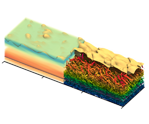
  $R = (\rho _p - \rho _a)/\rho _a$ to be small such that the Boussinesq approximation applies. Figure 1 shows span-averaged concentration at one instant in time for (a) supercritical and (b) subcritical currents. Quantities with tilde $(\,\tilde {\cdot }\,)$ denote variables scaled with bulk inlet parameters.

Figure 1. Scaled span-averaged concentration for (a) supercritical and (b) subcritical cases. White contours denote  $\tilde {c}=0.01$. Scaled momentum balance contributions together with turbulent structures and interface for supercritical (R20 – left panels, c,e,g) and subcritical (R200 – right panels, d, f,h) cases. Each panel contains: (i) section of the current showing the corresponding term of the momentum balance in volumetric representation (left of each panel); and (ii) turbulent structures and interface represented by isosurface of constant $\tilde {\lambda }_{{ci}}=0.06$ (coloured by $\tilde {z}$) and concentration $\tilde {c}=0.01$, respectively (in yellow). Also shown are: $\tilde {u}_{{max}}$, the location of the velocity maximum; and $\tilde {z}|_{\bar {P}=0}$, planes of zero turbulent kinetic energy production (light pink and violet planes). L and G indicate loss and gain of momentum, respectively.
We solve the mass, momentum and concentration equations (Salinas et al. Reference Salinas, Balachandar and Cantero2021a) using the highly scalable, higher-order spectral element solver Nek5000. We enforce a no-slip condition at the bottom boundary for the velocity field, and a zero gradient in the bed-normal direction for the concentration field. At the top ( $z=L_z$) and the outflow ( $L_x$) boundaries, we use open boundary conditions (Hu Reference Hu1996). Finally, we use periodic boundary conditions in the spanwise direction $y$. The domain is discretized using hexahedral elements with Gauss–Lobatto–Legendre (GLL) grid points on each element. We present details on domain size and grid resolution for each simulation in table 1, together with the inlet Richardson number ${Ri}_{in}$. For all cases, inlet Reynolds number ${Re}_{in}={Q}_{in}/\nu =5620$. DNS and LES are named ‘RX’ and ‘RXL’, respectively, where X is $1/S$. LES were performed using a modal explicit filtering for numerical stability.
Table 1. Details of simulations performed: case name, inlet Richardson number, domain size, number of spectral elements, number of GLL points per element, and total number of grid points.

Towards the goal of obtaining a reduced-order representation, we start with the following time- and span-averaged mass, agent concentration, streamwise momentum and mean kinetic energy equations:
 \begin{equation} \dfrac{\partial u}{\partial x} + \dfrac{\partial w}{\partial z} = 0 , \quad \dfrac{\partial uc}{\partial x} + \dfrac{\partial wc}{\partial z} ={-} \dfrac{\partial \langle u'c' \rangle}{\partial x} - \dfrac{\partial \langle w'c'\rangle}{\partial z} , \end{equation}
 \begin{equation} {\dfrac{\partial u^{2}}{\partial x}} + \underline{\dfrac{\partial uw}{\partial z}} ={-} \dfrac{1}{\rho} \dfrac{\partial p}{\partial x} - \dfrac{\partial \langle u'^{2} \rangle}{\partial x} - \underline{\dfrac{\partial \langle u' w'\rangle}{\partial z}} + \nu \left( \dfrac{\partial^{2} u}{\partial x^{2}} \right) + \underline{\nu \left( \dfrac{\partial^{2} u}{\partial z^{2}} \right)} + {Rcg \sin \theta} , \end{equation}
 \begin{align} \dfrac{1}{2}\dfrac{\partial u^{3}}{\partial x} + \dfrac{1}{2}\dfrac{\partial u^{2}w}{\partial z} &={-} \dfrac{1}{\rho} \dfrac{\partial pu}{\partial x} - \dfrac{\partial u \langle u'^{2} \rangle}{\partial x} - \dfrac{\partial u\langle u' w'\rangle}{\partial z} + \dfrac{\nu}{2} \left( \dfrac{\partial^{2} u^{2}}{\partial x^{2}} + \dfrac{\partial^{2} u^{2}}{\partial z^{2}} \right) + \dfrac{p}{\rho} \dfrac{\partial u}{\partial x} \nonumber\\ & \quad + \langle u'^{2} \rangle \dfrac{\partial u }{\partial x} + \langle u' w'\rangle \dfrac{\partial u }{\partial z} - {\nu} \left( \left( \dfrac{\partial u}{\partial x}\right)^{2} + \left( \dfrac{\partial u}{\partial z} \right)^{2} \right) + Rcug \sin \theta, \end{align}
where  $\boldsymbol {u} = \{ u, v, w\}$ is the velocity and $p$ is the pressure. Quantities within $\langle \cdot \rangle$ are averages over $y$ and $t$; we drop them for first-order statistics to simplify notation (i.e. $u = \langle u \rangle$). Perturbations are denoted with a prime; $\nu$ is the constant kinematic viscosity of the fluid; and $g$ is acceleration due to gravity. The underlined terms are discussed in § 2.1.
We define streamwise fluxes of mass, momentum and buoyancy as
 \begin{equation} Q(x) = \int_0^{\infty} u \, {\rm d}z \, , \quad M(x) = \int_0^{\infty} u^{2} \, {\rm d}z \, , \quad F(x) = \int_0^{\infty} Rcu g \sin \theta \, {\rm d}z . \end{equation}
In the simulations, the upper limit is replaced with a large value of  $z$ that extends far upwards into the ambient, where the current velocity and buoyancy vanish. The fluxes are used to define current height, mean velocity and buoyancy scales as (Craske & van Reeuwijk Reference Craske and van Reeuwijk2015a)
 \begin{equation} H(x) = Q^{2}/M , \quad U(x) = M/Q , \quad {B(x) = \int_0^{\infty} Rcg \sin \theta \, {\rm d}z = {FQ}/{(\theta_m M)}} . \end{equation}
 A conserved current is defined as one where the total amount of excess weight of the current remains independent of  $x$ and the buoyancy flux remains a constant. The buoyancy scale $B(x)$ varies along the streamwise direction. The shape factor $\theta _m=1$ when the $z$-variation of both velocity and concentration are the same. Thus, $\theta _m \ne 1$ is a measure of the difference in the vertical structure of $u(z)$ and $c(z)$. In the case of an unbounded plume, where both $u(z)$ and $c(z)$ are Gaussian, $(\theta _m-1)$ is a measure of the difference in their Gaussian width. In a gravity current, although the shapes of the velocity and concentration profiles are different, we observe $\theta _m \approx 1$.
We integrate the averaged equations in the  $z$-direction to obtain
 \begin{align} \dfrac{{\rm d} Q}{{\rm d}\kern0.06em x} = e_w \dfrac{M}{Q} , \quad \dfrac{{\rm d} \theta_g F}{{\rm d}\kern0.06em x} = 0 , \quad \dfrac{{\rm d} \beta_g M}{{\rm d}\kern0.06em x} ={-}C_D \dfrac{M^{2}}{Q^{2}} + \dfrac{FQ}{\theta_m M} ,\quad \dfrac{{\rm d} \gamma_g M^{2}/Q}{{\rm d}\kern0.06em x} = F + \delta_g \dfrac{M^{3}}{Q^{3}} . \end{align}
These are equivalent to the integral equations proposed by Parker, Fukushima & Pantin (Reference Parker, Fukushima and Pantin1986), except in that: (i) no ‘boundary-layer approximation’ (i.e.  $u \gg w$ and $\partial /\partial z \gg \partial /\partial x$) and (ii) no ‘top-hat’ assumption (i.e. simplified shape factors) have been used above. In the mass balance we have used the central assumption of entrainment that $w_e(x,z\rightarrow \infty ) = -e_w(x) U(x)$. In the momentum equation, the drag coefficient is defined as
 \begin{equation} C_D \dfrac{M^{2}}{Q^{2}} = C_D U^{2} = {\nu \left( \dfrac{\partial u}{\partial z} \right)_{z=0}}+ {\nu \dfrac{{\rm d}^{2} Q}{{{\rm d}\kern0.06em x}^{2}}} . \end{equation}
 All the simulation results show that  $C_D$ is dominantly determined by the first term on the right-hand side. In addition, the following definitions have been introduced:
 \begin{equation} \int_0^{\infty} ({p}/{\rho})\,{\rm d}z = \beta_p M , \quad \int_0^{\infty} \langle u'^{2} \rangle \,{\rm d}z = \beta_f M , \quad \beta_g = 1+\beta_p + \beta_f . \end{equation}
As defined above,  $\beta _p$ and $\beta _f$ account for both (i) the scaling of pressure versus $U^{2}$ and $\langle u'^{2} \rangle$ versus $U^{2}$ and (ii) differences in the shape of the pressure and Reynolds stress distributions compared to that of $u^{2}(z)$. In the concentration equation,
 \begin{equation} \int_0^{\infty} R \langle u' c' \rangle g \sin\theta \, {\rm d}z = \theta_f F \quad \text{and} \quad \theta_g = 1 + \theta_f . \end{equation}
Here,  $\theta _f$ accounts for streamwise Reynolds flux of concentration and we observe its contribution along with that of turbulent Reynolds stress to be generally small.
The mean kinetic energy equation substantially simplifies with the following shape-factor definitions:
 \begin{gather} \frac{1}{2} \int_0^{\infty} \left( u^{3} + \frac{pu}{\rho} + u \langle u'^{2} \rangle \right) \, {\rm d}z = ( \gamma_m + \gamma_p + \gamma_f ) \frac{M^{2}}{Q} = \gamma_g \frac{M^{2}}{Q} , \end{gather}
 \begin{gather} \int_0^{\infty} \left( \dfrac{p}{\rho} \dfrac{\partial u}{\partial x} + \langle u'^{2} \rangle \dfrac{\partial u}{\partial x} + \langle u'w' \rangle \dfrac{\partial u}{\partial z} \right) \, {\rm d}z = ( \delta_p + \delta_{f1} + \delta_{f2} ) \dfrac{M^{3}}{Q^{3}} = \delta'_{g} \dfrac{M^{3}}{Q^{3}} ,\nonumber\\ \dfrac{\nu}{2} \dfrac{{\rm d}^{2}M}{{{\rm d}\kern0.06em x}^{2}} + \dfrac{\nu}{2} \left. \dfrac{\partial u^{2}}{\partial z} \right|_{z=0} - \nu \int_0^{\infty} \left( \left( \frac{\partial u}{\partial x} \right)^{2} + \left(\frac{\partial u}{\partial z} \right)^{2} \right) \, {\rm d}z = \delta_v \dfrac{M^{3}}{Q^{3}} , \quad \delta_g = \delta'_g + \delta_v . \end{gather}
In (2.10),  $\gamma _m$ is the velocity shape factor, whose value depends only on the shape of the ensemble-averaged velocity profile. If $p(z)$ has the same shape as $u^{2}(z)$, then $\gamma _p = 2\beta _p \gamma _m$. Similarly, if $\langle u'^{2}\rangle$ has the same shape as $u^{2}(z)$, then $\gamma _f = 2\beta _f \gamma _m$. Finally, all the delta functions in (2.11) are negative, as they account for loss of mean kinetic energy due to turbulence production, viscous diffusion and viscous dissipation effects. The downstream evolution of all the shape factors as a function of $x$ is presented in figure 2(a,b), for cases (a) R20L and (b) R400L, respectively. All the shape factors reach a constant value in the case of R20L, whereas in the subcritical case of R400L $\beta _g$ and $\delta _g$ are still slowly evolving, but the observed trend suggests slow approach to a constant value.

Figure 2. Shape factors as a function of  $x$ for cases (a) R20L and (b) R400L. Depth-averaged momentum balance as a function of $x$ for cases (c) R20L and (d) R400L.
With these definitions, we can evaluate the different terms of the depth-averaged momentum balance (2.6a–d), which is presented in figure 2(c,d). In the momentum balance,  $FQ/(\theta _m M)$ is the source of streamwise momentum, which is balanced by basal drag $C_D M^{2}/Q^{2}$ and ${\rm d}(\beta _g M)/{{\rm d}\kern0.06em x}$. By writing the latter as $\beta _g e_w M^{2}/Q^{2} + Q \,{\rm d}(\beta _g U)/{{\rm d}\kern0.06em x}$, we understand it to account for both interface drag (dashed blue lines in figure 2c,d) and momentum sink/source due to acceleration/deceleration of the current (dash-dotted blue lines). In the supercritical case (R20L), a larger fraction of momentum source goes to interface drag due to intense mixing, while in the subcritical case (R400L), basal drag is the dominant sink of streamwise momentum. In both cases, the flow first decelerates near the inlet, until $Q\,{\rm d}(\beta _g U)/{{\rm d}\kern0.06em x}$ reaches negligible values far downstream, indicating that both flows are neither accelerating nor decelerating, especially in comparison with the other terms of the momentum balance.
2.1. Slow evolution to near-self-similar state
The evolution of the current towards self-similarity is demonstrated in figure 3, where the scaled profiles of streamwise velocity, concentration, and gradient and flux Richardson numbers, which are defined as
 \begin{equation} Ri_g=\frac{-R g_z \partial c/\partial z} { (\partial u/\partial z)^{2}} \quad \text{and} \quad Ri_f=\frac{R g_x \langle u'c' \rangle+R g_z \langle w'c' \rangle}{\langle u'w'\rangle \partial u/\partial z}, \end{equation}
are shown. After the initial adjustment of the profiles seen in red for R20L and in blue for R400L over the range  $50\leq x < 650$, we see an excellent collapse of the profiles of streamwise velocity, concentration and gradient Richardson number sufficiently far from the inlet – the last three profiles at $x = 650$, 700 and 750 are highlighted. A good collapse of the profiles in the self-similar state can be observed in both the interface and the near-bed layers. Note that near the streamwise velocity maximum, $Ri_g, Ri_f\rightarrow \infty$ as mean velocity gradient goes to zero. For the flux Richardson number, also a good collapse can be observed. However, in the subcritical case, both the numerator and the denominator in the definition of $Ri_f$ (2.12a,b) go to zero in the turbulence-free interface layer, preventing a reliable quantification, and therefore not shown.

Figure 3. Scaled (a) streamwise velocity  $u/U$, (b) concentration $c/C_b$ ( $C_b$ is basal concentration), (c) gradient Richardson number $Ri_g$ and (d) flux Richardson number $Ri_f$, as functions of scaled height $z/H$, for the supercritical case R20L and the subcritical case R400L. Red and blue profiles show the evolution in the interval $50\leq x < 650$, for cases R20L and R400L, respectively. For each quantity, we also show three profiles (in green, blue and orange) at the downstream locations of $x = 650$, 700 and 750. Their overlap, when compared to their earlier evolution, provides support for the approach to self-similarity. Note that, in the subcritical case R400L, both the numerator and the denominator in the definition of $Ri_f$ (2.12a,b) go to zero in the turbulence-free interface layer, preventing a reliable quantification, and therefore not shown.
In (2.6a–d), the first three can be interpreted as governing equations of  $Q$,
$Q$,  $F$ and $M$, while the last equation is the energy constraint that must be satisfied. The equations can be solved by assuming the shape factors to take constant values in the self-similar regime $(\beta _{g0}, \theta _{m0}, \theta _{g0}, \gamma _{g0}, \delta _{g0})$. With constant values for entrainment coefficient $e_{w0}$ and drag coefficient $C_{D0}$, we obtain $Q(x) \sim Q_1 x$ and $M(x) \sim M_1 x$ as the leading-order solution with
 \begin{align} Q_{1} = e_{w0} \{F/[\theta_{m0}(\beta_{g0} e_{w0} + C_{D0})]\}^{{1}/{3}} , \quad M_{1} = e_{w0} \{F/[\theta_{m0}(\beta_{g0} e_{w0} + C_{D0})]\}^{{2}/{3}} . \end{align}
These definitions can also be presented as  $Q_1 = e_{w0} U_0$ and $M_1 = e_{w0} U^{2}_0$, where
 \begin{equation} U_{0} = F^{1/3} \{ ({\gamma_{g0} - \beta_{g0} \, \theta_{m0}})/[{\theta_{m0} (C_{D0} \, \gamma_{g0} + \delta_{g0} \, \beta_{g0})}] \}^{1/3} \end{equation}
is the velocity of the current in the self-similar state, which depends not only on the slope but also on  $F$.
$F$.
The approach to self-similar behaviour is shown in figure 4(a–d), where  $Q(x)/Q_{in}$, $M(x)/M_{in}$, $H(x)/H_{in}$ and $B(x)/F^{2/3}$ are plotted for the seven cases considered. The agreement between the DNS and LES cases is clear. For all cases, $x = 750$ is large enough that the plots have sufficiently approached their linear behaviour in the self-similar state. In the self-similar state, the streamwise flux of mass and momentum go as $Q_1 x$ and $M_1 x$, while the height of the current goes as $H(x) \sim e_{w0} x$ (see (2.19)). The leading-order solutions for $Q/Q_{in}$, $M/M_{in}$ and $H/H_{in}$ are shown in figure 4(a–c) as dashed grey lines. On the other hand, the depth-averaged velocity reaches a constant value of $U(x) \sim U_0$ (figure 4e). While the behaviour of normalized current height is similar to those of $Q$ and $M$, the current velocity exhibits an oscillatory approach to unity in the supercritical currents. Furthermore, the bulk Richardson number
 \begin{equation} {Ri} = \frac{1}{S}\int_0^{\infty} Rcg \sin \theta \,{\rm d}z/U^{2} = \frac{F/\theta_m}{S Q^{3}/M^{3}} \end{equation}
slowly approaches a constant value of  ${Ri}_0$ (figure 4f) in both the subcritical and supercritical cases. It is interesting to note that the approach to self-similarity in all cases is through slow, ever-decreasing, acceleration of the current, as indicated by the fact that ${Ri}$ approaches ${Ri}_0$ from above.

Figure 4. Streamwise evolution of (a)  $Q(x)/Q_{in}$, (b) $M(x)/M_{in}$, (c) $H(x)/H_{in}$, (d) $B(x)/F^{2/3}$, (e) $U(x)/U_0$ and ( f) ${Ri}(x)$. Dashed grey lines show slopes in the self-similar state obtained from (2.13a,b) and (2.19). Dash-dotted horizontal lines in ( f) show $Ri_0$ for each slope.
It must be stressed that the depth-averaged equations (2.6a–d) are exact, since all the terms of the Navier–Stokes equations are retained and included in the definitions of the different shape factors. Each term of the momentum and kinetic energy equations, calculated in the DNS and LES as a function of  $x$, is averaged over a short extent along the streamwise direction and the results are shown in figure 5(a,b). Owing to the exactness of the equations, perfect momentum and energy balances are observed.

Figure 5. Scaled mean (a) momentum and (b) energy balance for all cases in the near-self-similar state. Sinks are shown in blue and violet (left) and sources in orange (right). (c) Energy constraint on entrainment: left- and right-hand sides of (2.17);  $\boldsymbol {\lozenge }$ shows $(1/2)e_{w0}$ given in (2.19).
Figure 1 presents the three-dimensional structure of the supercritical (panels c,e,g) and subcritical (panels d, f,h) currents in the near-self-similar state (section in dashed red box in figure 1a,b). The left half of panels (c–f) show a volumetric visualization of the two underlined terms on the right-hand side of (2.2), with panels (g,h) showing the underlined term on the left-hand side. In the right half of each panel, the interface between the current and the ambient marked by  $\tilde {c}=0.01$ is shown (in yellow) with the three-dimensional vortical structures identified by contours of swirling strength $\tilde {\lambda }_{{ci}}$ (Zhou et al. Reference Zhou, Adrian, Balachandar and Kendall1999; Chakraborty, Balachandar & Adrian Reference Chakraborty, Balachandar and Adrian2005) (coloured by $\tilde {z}$ – see zoom-in views I and II).
In the panels, we focus on three important aspects that are of most relevance. (i) The interface with the ambient is highly turbulent in the supercritical current while it is very flat and non-turbulent in the subcritical current. (ii) In panels (d, f,h) (subcritical current), two horizontal surfaces of zero turbulent production marked as  $\tilde {z}|_{\bar {P}=0}$ are shown. The layer of fluid between these planes is termed ‘destruction layer’, since turbulence production is negative, and is the result of the interaction between near-wall hairpins (‘HP’ in zoom-in view I) and counter-rotating vortices (‘CV’) (see Salinas et al. Reference Salinas, Balachandar, Shringarpure, Fedele, Hoyal, Zu niga and Cantero2021b). (iii) Comparing the different terms of the momentum equation, it can be seen that in the interface layer (above the maximum of velocity), the balance is mainly between $\partial (\tilde {u}\tilde {w})/\partial \tilde {z}$ (zoom-in view IV) and $\partial (\langle \tilde {u}'\tilde {w}' \rangle )/\partial \tilde {z}$ (zoom-in view III) in the supercritical current, while it is between $\partial (\tilde {u}\tilde {w})/\partial \tilde {z}$ (zoom-in view VI) and $\partial ^{2}\tilde {u}/\partial \tilde {z}^{2}/Re_{{in}}$ (zoom-in view V) in the subcritical current. In other words, ‘turbulence’/‘viscous diffusion’ is responsible for the entrainment of ambient fluid into the ‘supercritical’/‘subcritical’ current.
2.2. Energy-consistent entrainment relation
Following the steps of Craske & van Reeuwijk (Reference Craske and van Reeuwijk2015a), using the chain rule we can write
 \begin{equation} e_w = \dfrac{Q}{M} \dfrac{{\rm d}Q}{{\rm d}\kern0.06em x} = {\dfrac{2}{\beta_g} \dfrac{Q^{2}}{M^{2}} \dfrac{{\rm d} \beta_g M}{{\rm d}\kern0.06em x}} {- \dfrac{Q^{3}}{\gamma_g M^{3}} \dfrac{{\rm d}}{{\rm d}\kern0.06em x} \left( \gamma_g \dfrac{M^{2}}{Q} \right)} {+ \dfrac{Q^{2}}{M} \dfrac{{\rm d}}{{\rm d}\kern0.06em x} \left( \ln \left( \dfrac{\gamma_g}{\beta_g^{2}} \right) \right)} . \end{equation}
The three contributions come from (i) streamwise variation of current momentum, (ii) streamwise variation of mean kinetic energy (mKE) and (iii) streamwise variation of the various shape factors. Substituting the momentum and kinetic energy equations in the above expression, we obtain the final energy-consistent entrainment expression as
 \begin{equation} \frac{1}{2}e_w + \dfrac{C_D}{\beta_g} = {-\dfrac{\delta_g}{2\gamma_g}} + {{Ri} S \left( \dfrac{1}{\beta_g} - \dfrac{\theta_m}{2\gamma_g} \right)} + { \dfrac{1}{2} \dfrac{Q^{2}}{M} \dfrac{{\rm d}}{{\rm d}\kern0.06em x} \left( \ln \left( \dfrac{\gamma_g}{\beta_g^{2}} \right) \right)} . \end{equation}
 Equation (2.6a–d) is a reduced-order framework for rapid evaluation of the current's evolution. However, closure models of shape factors  $\beta _g$, $\theta _m$, $\theta _g$, $\gamma _g$ and $\delta _g$, along with models of $e_w$ and $C_D$, are needed. Since (2.6a–d) have been demonstrated to be exact, the accuracy of prediction depends only on the fidelity of the closure models. The expression given in (2.17) is an important energy constraint that must be satisfied by the closure models – this constraint is always valid, even when the current is not self-similar.
Simpler relations can be obtained under conditions of near-self-similarity. The mass and momentum balances and similarly the mass and kinetic energy balances can be combined to obtain the following two different expressions of self-similar entrainment coefficient:
 \begin{equation} e_{w0} = ({Ri}_0 S - C_{D0})/\beta_{g0} \quad \text{and} \quad e_{w0} = (\theta_{m0} {Ri}_0 S + \delta_{g0})/{\gamma_{g0}} . \end{equation}
Equating the above two equations, we obtain the following third equivalent expression:
 \begin{equation} e_{w0} = (\delta_{g0} + C_{D0} \theta_{m0})/(\gamma_{g0} - \beta_{g0} \theta_{m0}), \end{equation}
which depends only on the self-similar shape factors and  $C_{D0}$. These relations satisfy the general condition (2.17). The first relation in (2.18a,b) is the easiest to interpret. The streamwise driving force exerted on the current due to the excess weight goes as ${Ri}_0 S U_0^{2}$. This driving force is exactly balanced by basal drag $C_{D0} U_0^{2}$ and the entrainment drag $\beta _{g0} e_{w0} U_0^{2}$, which is due to the fact that the quiescent ambient fluid when brought into the current must move at self-similar streamwise velocity $U_0$. The second relation in (2.18a,b) implies that the work done by gravity scales as $\theta _{m0} {Ri}_0 S$, and it is balanced by (i) mKE lost to turbulence, (ii) mKE lost to dissipation and (iii) mKE supplied to entrained ambient fluid. The first two losses are represented by $\delta _{g0}U^{2}_0$, while the third loss is captured by $\gamma _{g0} e_{w0}U^{2}_0$. The balance between the different terms of (2.17) in the near-self-similar state is shown in figure 5(c), where the right-hand side terms are $E_{loss}$, $E_{Ri}$ and $E_{ss}$. The difference between the blue/orange and purple/green bars indicates the small effect of $E_{ss}$. Also presented is the entrainment coefficient computed from (2.19) (blue diamonds). We see good agreement between the values of $(1/2) e_{w0}$ obtained directly from our simulations and obtained indirectly through (2.19).
2.3. Slope dependence of entrainment, Richardson number and shape factors
The self-similar shape factors are only functions of the bed slope  $S$ and this dependence is shown in figure 6(a–c), where the symbols are shape factors obtained from the seven simulations. Plots of shape factors as functions of $x$ obtained from the DNS and LES were fitted to obtain their asymptotic $x\rightarrow \infty$ values, which are shown in figure 6(a–c). The proposed models of $\beta _{g0}(S)$, $\theta _{m0}(S)$, $\gamma _{g0}(S)$, $\delta _{g0}(S)$ and $C_{D0}(S)$ are also shown. We caution that these fits are approximate and they cover only a small range of bed slope. With increasing slope, $\beta _{g0}$ and $\gamma _{g0}$ decrease and approach the limiting values of $1.0$ and $0.5$. On the other hand, $\delta _{g0}$ and $C_{D0}$ increase with increasing $S$, indicating enhanced dissipation, and $\theta _{m0}$ also increases with $S$, although its value remains close to unity. The dependence of $U_0/F^{1/3}$ along with $Q_1/F^{1/3}$ and $M_1/F^{2/3}$ are presented in figure 6(d–f). All three quantities are nearly constant in the subcritical regime, but decrease (or increase) in the supercritical regime. Dashed red lines in these panels are plots of models obtained from (2.13a,b) and (2.14).

Figure 6. Various near-self-similar shape factors and quantities plotted as a function of bed slope: (a)  $\theta _{m0}$, (b) $\beta _{g0}$ and $\gamma _{g0}$, (c) $|\delta {g0}|$ and $C_{D0}$, (d) $U_0/F^{1/3}$, (e) $Q_1/F^{1/3}$ and ( f) $M_1/F^{2/3}$. The blue dashed and orange dashed lines are best fits of our data; the red dashed lines are derived models (see (2.13a,b) and (2.14)).
Substituting (2.19) for  $e_{w0}$ into (2.18a,b), we obtain the self-similar value of $Ri$ (see (2.15))
 \begin{equation} {Ri}_{0} = ({C_{D0} \gamma_{g0} + \delta_{g0} \beta_{g0}})/[{S (\gamma_{g0} - \beta_{g0} \theta_{m0})}] , \end{equation}
which can be recast as densimetric Froude number  ${Fr}_0 = 1/\sqrt {{Ri}_0}$. In figure 7(a), ${Fr}_0$ as a function of $S$ is plotted along with experimental data. The demarcation of subcritical and supercritical currents at ${Fr} = 1$ is also shown. In the inset we present ${Ri}_0(S)$, where the red line is obtained by plotting (2.20) with the proposed models of the various shape factors. In figure 7(b), in the inset we plot $e_{w0}(S)$. Again, the symbols are the simulation results, while the red line is a plot of (2.19). Figure 7(b) shows $e_{w0}$ plotted as a function of ${Ri}$. Results from experimental data are also plotted, along with the correlations of Turner and Parker. Self-similar $e_{w0}$ is lower and appears to follow a power law. Also plotted are $e_{w,n}$ obtained at the first normal condition downstream of the inlet (Salinas et al. Reference Salinas, Cantero, Shringarpure and Balachandar2019), which are in good agreement with the correlation of Parker et al. (Reference Parker, Garcia, Fukushima and Yu1987). Clearly, entrainment decreases from this near-inlet normal value to the self-similar value.

Figure 7. (a) Densimetric Froude number as a function of slope  $S$ (blue symbols). The orange and green dashed lines are the models of Sequeiros (Reference Sequeiros2012) and Stacey & Bowen (Reference Stacey and Bowen1988), respectively. The grey circles are data from multiple sources obtained from Sequeiros (Reference Sequeiros2012). (b) Entrainment $e_w$ as a function of $Ri$ (blue symbols). The black and green dashed lines are the models of Parker et al. (Reference Parker, Garcia, Fukushima and Yu1987) and Turner (Reference Turner1986), respectively. The grey symbols are experimental data from different sources (see Salinas et al. Reference Salinas, Cantero, Shringarpure and Balachandar2019). The red dashed lines are derived models (see (2.19) and (2.20)).
3. Conclusions
Results of well-resolved DNS and LES performed over very long streamwise lengths show that gravity currents slowly approach a near-self-similar state over a wide range of bed slope that covers both the subcritical and supercritical regimes. The near-self-similar state is characterized by slowly varying flow parameters. As the current evolves towards the self-similar state,  $Ri$,
$Ri$,  $e_w$, velocity scale and basal drag coefficient approach constant values, while the current height, volume and momentum fluxes continue to increase linearly. These self-similar values only depend on the bed slope $S$ and sediment flux, and their variation is presented for a range of slopes in figure 6. Only the velocity scale $U$ depends additionally on the buoyancy flux as $U \sim F^{1/3}$.
The approach to self-similarity is slower in subcritical currents, compared to their supercritical counterparts. The approach to self-similarity in all cases is through slow, ever-decreasing, acceleration of the current, as indicated by the fact that  ${Ri}$ approaches ${Ri}_0$ from above. The self-similar value of entrainment appears to follow a power law and its value is lower than the entrainment correlation of Parker et al. (Reference Parker, Garcia, Fukushima and Yu1987) and the near-inlet normal value. Following the work of Craske & van Reeuwijk (Reference Craske and van Reeuwijk2015a), we derive an energy-consistent entrainment relation, whose limiting form in the self-similar limit is also explored. We also discuss these results in the context of ‘exact’ depth-averaged equations. The approach to self-similarity is slow and thus the simulations require a very long computational domain that extends over several hundred current heights along the streamwise direction. Even much longer domains are required to firmly establish the self-similar values. Future work is needed to investigate slopes that are beyond the range considered here and also to study the rapid evolution of currents in supercritical and subcritical slopes when disturbed from their self-similar value.
Acknowledgements
The authors would like to thank ExxonMobil for their support. S.L.Z and M.I.C. would also like to acknowledge CONICET, CNEA and UNCuyo.
Declaration of interests
The authors report no conflict of interest.


 Open access