


1. Introduction
Gravity-driven film flow along a flat inclined wall is a basic paradigmatic flow configuration that is encountered in numerous environmental and biological systems (Craster & Matar Reference Craster and Matar2009), as well as in countless industrial processes (Alekseenko, Nakoryakov & Pokusaev Reference Alekseenko, Nakoryakov and Pokusaev1994; Rocha, Bravo & Fair Reference Rocha, Bravo and Fair1996; Vlachogiannis & Bontozoglou Reference Vlachogiannis and Bontozoglou2002; Xu et al. Reference Xu, Singh, Bao and Wang2019). In many industrial applications, such as distillation columns, films flow along structured packings to enhance heat or mass transfer (Rocha et al. Reference Rocha, Bravo and Fair1996). Transfer rates can be raised significantly by travelling waves, which occur as a result of the primary instability of the steady film flow already at low Reynolds numbers (Chang & Demekhin Reference Chang and Demekhin2002). Surface renewal with transfer enhancement can also be induced by wave breaking, which is an example for turbulence being generated at the free surface (Brocchini & Peregrine Reference Brocchini and Peregrine2001). For film flow along smooth walls, particularly with the occurrence of turbulent surface waves, transfer rates increase considerably (Roberts & Chang Reference Roberts and Chang2000; Park et al. Reference Park, Nosoko, Gima and Ro2004). Here, turbulence first occurs in the form of three-dimensional solitary-wave pulses (Demekhin et al. Reference Demekhin, Kalaidin, Kalliadasis and Vlaskin2007). Transfer can be enhanced further by the proper choice of the wall topography and the process parameters (Rocha et al. Reference Rocha, Bravo and Fair1996; Åkesjö et al. Reference Åkesjö, Gourdon, Vamling, Innings and Sasic2019). To optimize transfer rates, for instance, it is necessary to improve our understanding of the flow regimes in the film and the impact of the structured substrate topography (Valluri et al. Reference Valluri, Matar, Hewitt and Mendes2005). Here, we report on surface turbulence in film flows along sinusoidal contours at Reynolds numbers of order 10. We show that the turbulent waves are different from the solitary waves that emerge from the primary instability of the steady flow.
Gravity-driven film flow over inclined periodic topographies has been studied for a wide parameter range. At small waviness, thin film flow is essentially akin to that over a flat incline at the respective local inclination angle, yet deviations increase at small inclination angles where the slope becomes non-monotonic (Wierschem, Lepski & Aksel Reference Wierschem, Lepski and Aksel2005; Mukhopadhyay & Mukhopadhyay Reference Mukhopadhyay and Mukhopadhyay2020). Eddies form in the troughs at higher corrugation steepness (Wierschem, Scholle & Aksel Reference Wierschem, Scholle and Aksel2003; Wierschem et al. Reference Wierschem, Pollak, Heining and Aksel2010), and capillary forces become relevant at short wavelengths (Aksel & Schörner Reference Aksel and Schörner2018). When inertia becomes relevant, hydraulic jumps and resonance with the substrate topography occur (Wierschem & Aksel Reference Wierschem and Aksel2004; Heining et al. Reference Heining, Bontozoglou, Aksel and Wierschem2009; Wierschem et al. Reference Wierschem, Pollak, Heining and Aksel2010), and travelling waves may break (Dauth & Aksel Reference Dauth and Aksel2018, Reference Dauth and Aksel2019). At Reynolds numbers beyond 1000, turbulent films have been reported in flow along periodic undulations of 5–10 cm wavelength at large (Zeng et al. Reference Zeng, Wang, Li, Wei, Yu, Wang, Wang, Hou and Yuan2023) and small (Plumerault, Astruc & Thual Reference Plumerault, Astruc and Thual2010) inclination angles. Further details on the rich phenomenology of gravity-driven films flowing over topography may be found in the recent review by Aksel & Schörner (Reference Aksel and Schörner2018).
Here, we focus on gravity-driven turbulent film flow that is generated during the flow over periodic ripples. We observe this regime beyond the breaking of solitary waves reported by Dauth & Aksel (Reference Dauth and Aksel2018). They studied the impact of substrate amplitude and wavelength as well as that of the perturbation frequency, and found air entrainment by wave breaking. In a follow-up report, they showed that the waves break irregularly already at Reynolds numbers between approximately 10 and 20 (Dauth & Aksel Reference Dauth and Aksel2019). Apart from air entrainment, the breaking was accompanied by fingering and droplet generation, and the irregular fronts tend to widen with inclination angle and Reynolds number. Compared to the system studied by Dauth & Aksel, we use a silicon oil with a ten times lower viscosity, higher inclination angle and shorter substrate corrugations, resulting in thinner films at the same Reynolds number, and a more severe impact of the substrate contour on the flow. This results in a clear change in the flow regime, which appears to be capillary turbulence.
Surface-wave turbulence has been studied intensively during the last decades. Usually deep-sea capillary–gravity waves are considered (Hasselmann Reference Hasselmann1962; Deike, Berhanu & Falcon Reference Deike, Berhanu and Falcon2014; Falcon & Mordant Reference Falcon and Mordant2022). In the laboratory, turbulence of surface waves has been studied in deep vessels excited with wave makers; see e.g. the recent review by Falcon & Mordant (Reference Falcon and Mordant2022) and references therein. The energy transfer from the band of forcing frequencies to small, dissipative scales takes the form of an energy cascade. For weakly turbulent systems, the power spectral density of the wave elevation follows characteristic power laws sufficiently far away from the forcing frequencies (Falcon & Mordant Reference Falcon and Mordant2022). The exponent depends on the minimum number of waves involved in the energy transfer. For capillary waves, it ranges from  $-17/6$ for three-wave resonant interaction to $-31/12$ for interaction of five waves (Ricard & Falcon Reference Ricard and Falcon2021). With increasing viscosity, however, the power spectral density steepens, particularly at lower energy input (Deike et al. Reference Deike, Berhanu and Falcon2014).
Resonant wave interactions in free-surface flows can also be mediated by periodic bottom contours. This has been considered particularly in the framework of ripples in coastal areas of shallow slopes, where usually two-dimensional wave interactions in potential flow are considered (McHugh Reference McHugh1992; Fan et al. Reference Fan, Tao, Zheng and Peng2022). In the case considered in the present paper, however, the liquid film is rather thin, thus viscosity and dissipation at the bottom cannot be ignored. Furthermore, the breaking of travelling solitary-wave fronts results in fingers that may interact also spanwise to the main flow direction. Hence resonant interaction of a triad formed by a pair of oblique modes with the wavy bottom contour is expected to be relevant, as in the steady three-dimensional pattern further upstream in the same system reported recently (Al-Shamaa, Kahraman & Wierschem Reference Al-Shamaa, Kahraman and Wierschem2023) or in travelling waves in film flows down flat inclines or in boundary layers (Kachanov Reference Kachanov1994; Liu, Schneider & Gollub Reference Liu, Schneider and Gollub1995).
2. Experimental system and set-up
The experimental system was identical to that used by Al-Shamaa et al. (Reference Al-Shamaa, Kahraman and Wierschem2023). The channel is built from an aluminium bottom and Plexiglas sidewalls. The bottom has width  $170\ {\rm mm}$ and length $950\ {\rm mm}$. The first $895\ {\rm mm}$ of the bottom serves as a corrugated substrate, while the rest of it is flat. The substrate undulations have a sinusoidal contour in the main flow direction with wavelength $10\ {\rm mm}$ and amplitude $1\ {\rm mm}$. All experiments were carried out at a fixed channel inclination angle $\theta =45 \pm 0.1^\circ$ with respect to the horizontal. A sketch of the apparatus together with the set-ups is shown in figure 1.

Figure 1. (a) Side view of the experimental apparatus with the shadowgraph set-up. (b) Front view of the experimental apparatus with the light-sheet configurations.
Silicon oil ELBESIL ÖL B10 coloured with the fluorescent dye Quinizarin (Q906-100G, Sigma-Aldrich) was chosen to be the working liquid. Its physical properties were measured in a temperature interval ranging from  $296.15\ {\rm K}$ to $298.15\ {\rm K}$. All of our tests were implemented at temperature $297.15 \pm 0.3\ {\rm K}$. At this temperature, the silicon oil properties were: viscosity $\eta = 9.85 \pm 0.16\ {\rm mPa}\ {\rm s}$, density $\rho = 0.937 \pm 0.001\ {\rm g}\ {\rm cm}^{-3}$, and surface tension $\sigma = 19.56 \pm 0.06\ {\rm mN}\ {\rm m}^{-1}$. Hence the capillary length is $L_{Ca} = \sqrt {\sigma /( \rho g)} = 1.46\ {\rm mm}$. To ensure temperature uniformity during the experimental runs, the temperature was monitored by using a digital thermometer at the inlet and at the exit of the channel.
To assure a low level of initial fluctuations, we used an eccentric worm pump (Jöhstadt, Germany). As additional measures for damping fluctuations, the oil was transported from the pump through an approximately  $4\ {\rm m}$ long reinforced PVC hose to the inflow, where the flow direction was reversed and distributed evenly over the channel width. The mass flow rate $\dot {m}$ was measured by installing a gate of width $b=30\ {\rm mm}$ at the centreline of the flat part of the bottom near the outlet of the channel. The bulk Reynolds number was calculated from
 \begin{equation} Re=\frac{\dot{m}}{\eta b}. \end{equation}
In the present work, it ranged from approximately  $10$ to $60$, with a time-averaged film thickness $\delta$ of approximately $0.6$– $1.6\ {\rm mm}$ as obtained from the zeroth Fourier modes of the light-sheet data (see below) for the free surface and the bottom contour (Wierschem et al. Reference Wierschem, Pollak, Heining and Aksel2010). The vertical Kapitza number, defined as $Ka^*=\sigma / (\rho g^{1/3} \nu ^{4/3})$, was $42$. Here, $\nu$ is the kinematic viscosity. At the studied inclination angle, the Kapitza number $Ka=Ka^*/{\sin ^{1/3} \theta }$ was $48$.
$48$.
Two techniques were used to study the unsteady three-dimensional flow. We employ shadowgraphy to obtain general spatiotemporal information about the free surface and light-sheet technique to acquire time series about the local surface elevation. The set-up of the shadowgraph technique is shown in figure 1(a) (Al-Shamaa et al. Reference Al-Shamaa, Kahraman and Wierschem2023): the film surface was illuminated with the light of a  $400\ {\rm W}$ halogen lamp reflected from the laboratory ceiling. It was imaged with a monochrome camera ( $1280 \times 1024$ pixels, $8\ {\rm bit}$ resolution, frame rate $15\ {\rm fps}$). The camera was aligned perpendicularly to the channel bottom to capture the top view of the flow at three overlapping sections. Each section covers the entire width of the channel and approximately 23 % of the corrugated length of the channel. The upper section covers a distance from $330\ {\rm mm}$ to $565\ {\rm mm}$ from the channel inflow; the mid-section ranges from $510\ {\rm mm}$ to $710\ {\rm mm}$; and the lower section ranges from $636\ {\rm mm}$ to $845\ {\rm mm}$.
The light-sheet set-up is shown in figure 1(b). The light sheet was created using a blue laser (power  $0.04\ {\rm W}$, wavelength $450\ {\rm nm}$) with a cylindrical lens. The laser was aligned perpendicularly to the bottom at the centreline of the channel. Its light excites the fluorescent dye in the light sheet. The data were recorded with a monochrome camera ( $8\ {\rm bit}$ resolution). A green colour filter in front of the lens suppressed the scattered laser light while transmitting the fluorescent radiation. The camera was inclined with respect to the channel bottom to avoid interference with the meniscus or surface structures (Wierschem & Aksel Reference Wierschem and Aksel2004). The recorded data were calibrated with scaled paper. The pictures covered a length $7\ {\rm mm}$ around crests of the bottom undulation. We analysed time series of $8192$ frames at crest numbers 43 and 58, corresponding to distances $425\ {\rm mm}$ and $575\ {\rm mm}$ from the channel inflow, at frame rate $172.53\ {\rm fps}$. From the frames, the position of the free surface was determined at the peak of the crest with an edge detection code in MATLAB, as reported previously by Al-Shamaa et al. (Reference Al-Shamaa, Kahraman and Wierschem2023).
Droplets that form occasionally can be identified and tracked with the light-sheet technique. Their number increases with Reynolds number. Since we focus on the free surface of the film, we ignore them in the time series of the free surface position using linear interpolation. Yet their impact is rather small: at the highest Reynolds number studied, we could identify fewer than 300 droplets in the entire time series of more than  $8000$ frames. We analysed the time series of the unsteady free surface position by the power spectral density $S$:
$S$:
 \begin{equation} S=\frac{1}{T} \left\lvert \int_{0}^{T} h(t)\ {\rm e}^{{\rm i}2 {\rm \pi}ft}\,{\rm d}t \right\rvert^2, \end{equation}
where  $t$ is time, $T$ is the duration of the time series, and $h$ and $f$ are the positions of the free surface and the frequency, respectively (Falcon & Mordant Reference Falcon and Mordant2022).
3. Results and discussion
The tremendous impact of bottom ripples on the film flow shows the direct comparison at the same Reynolds number with a flat incline in figure 2. The flow down the flat incline in figure 2(a) shows the well-known instability of the steady flow into travelling solitary waves. These waves appear as localized humps with a steep front and a long tail. They result from the nonlinear dynamics of the flow. Different from classical solitons, they are dissipative (Liu & Gollub Reference Liu and Gollub1994). The flow over the corrugations in figure 2(b), on the contrary, is in the turbulent regime except near the inflow, where a steady three-dimensional pattern appears, which was studied by Al-Shamaa et al. (Reference Al-Shamaa, Kahraman and Wierschem2023).

Figure 2. Frontal view on the film flow over (a) a flat incline and (b) the bottom corrugations, at otherwise identical parameters. Flow is from top to bottom. Dark horizontal lines in (a) are travelling waves; in (b), regular short, bright vertical lines at the top are a steady three-dimensional surface pattern (Al-Shamaa et al. Reference Al-Shamaa, Kahraman and Wierschem2023). Here,  $Re=33$.
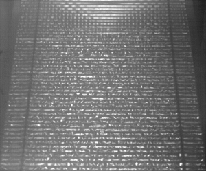
At the studied areas of the channel, travelling solitary-wave fronts appear from noise at the lowest Reynolds number studied; see figure 3(a). As seen in the figure, the wave fronts are already broken up into fingers, similar to what was reported by Dauth & Aksel (Reference Dauth and Aksel2019). The overhanging wave fronts are prone to air entrainment, which results in a strong perturbation of the flow (Dauth & Aksel Reference Dauth and Aksel2018). In our case, the fingers have typical width approximately  $8\ {\rm mm}$, i.e. smaller than $2 {\rm \pi}L_{Ca}$, and hence are apparently due to a capillary instability. Currently, it remains unclear whether it is a Rayleigh–Plateau instability or rather a Rayleigh–Taylor instability as found by Kofman, Mergui & Ruyer-Quil (Reference Kofman, Mergui and Ruyer-Quil2014) for solitary waves in films down steep inclines. Dauth & Aksel (Reference Dauth and Aksel2018) pointed out that the instability is affected by the streamwise scale of the bottom topography, as they did not find wave breaking if the corrugations were quite separate. Hence considering single steps up or down as done by Bontozoglou & Serifi (Reference Bontozoglou and Serifi2008) is not sufficient, and inertia seems to be relevant. In view of the steady three-dimensional pattern upstream (Al-Shamaa et al. Reference Al-Shamaa, Kahraman and Wierschem2023), resonance with the corrugations appears to promote wave breaking.

Figure 3. Top view of the channel as seen with the shadowgraph method. The section covers a distance between  $510\ {\rm mm}$ and $710\ {\rm mm}$ from the channel inflow over the entire channel width. Flow direction is from top to bottom. Straight horizontal lines are due to the bottom undulations; other brightness variations are due to free-surface variations. The arrow in (a) indicates crest number $58$. Here, $Re$ values are (a) $10$, (b) $15$,(c) $23$ and (d) $33$.
$33$.
With increasing Reynolds number, the number of the solitary-wave fronts tends to increase. As shown in figures 3(a,b), the wave fronts are already somewhat irregular. This is again in line with Dauth & Aksel (Reference Dauth and Aksel2019), who showed that subsequent wave fronts appear to be uncorrelated. In their case, the chaotic behaviour may appear even more striking as they generated the waves with a wave maker at fixed frequency. At higher Reynolds number, the waves break onto each other (see lower left in figure 3b) and the fronts tend to widen in line with the observations by Dauth & Aksel (Reference Dauth and Aksel2019). Increasing the Reynolds number further, more waves appear to cover the free surface. At  $Re=23$, only small regular patches remain on the free surface; see figure 3(c). Beyond this Reynolds number, these patches apparently disappear, and the free surface appears to be highly irregular; see figure 3(d). The average spanwise wavelength is mainly in a band between $6$ and $8\ {\rm mm}$, and tends to decrease slightly with increasing Reynolds number. In what follows, we will call this regime capillary turbulence.
Sidewalls have a damping impact, as shown recently by Kögel & Aksel (Reference Kögel and Aksel2020) and Mohamed, Sesterhenn & Biancofiore (Reference Mohamed, Sesterhenn and Biancofiore2023) for the primary instability. Yet impact and frequency at which damping is most relevant decrease with channel width and inclination angle. In our case, at inclination angle  $45^\circ$, and channel width to average film thickness ratio of the order of approximately 100, sidewalls have only a minor impact. They do not seem to have a noticeable effect beyond the width of the small-scale structures; see figure 3.
Figure 4 shows examples for the power spectral density of the free surface position for broken solitary-wave fronts and for capillary turbulence. Exemplary sequences of the time series are shown in the insets. For the solitary waves in figure 4(a), the maximum is  $0.29\ {\rm mm}^2\ {\rm Hz}^{-1}$, hence considerably higher than for the capillary turbulence. We cropped the power spectral density of the broken solitary-wave fronts in figure 4(a) to the maximum peak of the capillary turbulent regime in figure 4(b). Apart from the significant height difference of the maximum peaks, the power spectral densities of the two regimes differ in further aspects. While the maximum of the broken solitary waves occurs at frequency approximately $6\ {\rm Hz}$, there is no prominent peak at frequencies below $10\ {\rm Hz}$ in the capillary regime. Instead, the maximum occurs at much higher frequencies. Furthermore, the spectrum density of the broken solitary waves decays more steeply than for the capillary turbulence.

Figure 4. Power spectral density of the unsteady free-surface position for (a) broken solitary waves and (b) the capillary turbulent regime. Black lines show the power spectral density; white lines indicate the moving mean averaged over an interval of  $4\ {\rm Hz}$. The maximum for the broken solitary waves in (a) reaches a value $0.29\ {\rm mm}^2\ {\rm Hz}^{-1}$; the diagram was cropped to the maximum peak of (b). Insets show corresponding time series sections of the film thickness. Distance from channel inflow is $575\ {\rm mm}$, and $Re$ values are (a) $10$, and (b) $41$.
$41$.
The power spectral densities are strongly scattered. To analyse their trends over larger frequency ranges, we smoothed them by taking the moving mean over an interval of  $4\ {\rm Hz}$ as shown by white curves in figure 4. As is apparent from the figure, the maxima of the smoothed power spectral densities are considerably smaller than those of the unsmoothed ones. Yet general trends remain.
Figure 5(a) shows the maxima of the smoothed spectra as a function of Reynolds number; the unsmoothed data are provided in the Appendix, in figure 8. In the broken solitary-wave regime below  $Re=23$, the maximum first increases to $Re=16$, and then declines. In the capillary turbulent regime beyond $Re=23$, on the contrary, the maxima remain approximately constant at low levels up to Reynolds number approximately $47$, before they rise steadily at higher Reynolds numbers. The frequency at which the maximum in the smoothed power spectral density occurs confirms the differences between the two regimes; see figure 5(b). While the frequency rises linearly in the broken solitary-wave regime up to approximately $8\ {\rm Hz}$, it jumps at crossover to approximately $18\ {\rm Hz}$. In the capillary turbulent regime, the frequency data are more scattered, varying approximately within the band between the secondary maxima in figure 5(b). Nevertheless, from the crossover at $Re=23$, the data seem to increase further, up to $30\ {\rm Hz}$ at Reynolds number approximately $47$. The trends are the same for both locations studied. Only at Reynolds numbers beyond approximately $47$ does there appear to be a difference: particularly at crest number $58$, a linearly increasing frequency seems to reappear as a prolongation of the broken solitary-wave branch below $Re=23$. We hypothesize that solitary waves may gain relevance again at higher Reynolds numbers, where the film thickness is larger, resulting in a weaker impact of the bottom undulation on the free surface. We remark that the general trends are the same for the unsmoothed power spectral densities; see figure 8 in the Appendix.

Figure 5. (a) The maximum, and (b) its frequency, of the smoothed power spectral density as a function of Reynolds number. Data points show values from the moving mean averaged over an interval of  $4\ {\rm Hz}$. Solid and open symbols correspond to crest number $43$ and $58$, respectively. The dotted vertical lines indicate the crossover between broken solitary waves and capillary turbulence.
We note that the crossover from broken solitary waves to capillary turbulence at Reynolds numbers of approximately  $23$ coincides with the occurrence of a steady three-dimensional surface pattern further upstream; see figure 1(b). The average spanwise wavelength in the turbulent regime is slightly smaller than that of the steady pattern, where the wavelength was approximately $10\ {\rm mm}$ at $Re=30$, and decreased to approximately $9\ {\rm mm}$ at higher Reynolds numbers (Al-Shamaa et al. Reference Al-Shamaa, Kahraman and Wierschem2023).
Apart from the maximum, there are numerous local peaks in the power spectral density (figure 4). We expect them to occur due to nonlinear wave interaction (Falcon & Mordant Reference Falcon and Mordant2022). Yet in what follows, we focus on the small-scale trend of the energy cascade. To that end, we consider the moving mean averaged power spectral density as indicated by white lines in figure 4. In the high-frequency range, well beyond the forcing frequencies at the maximum peaks, the decay in the power spectral density is well described by a power law. Figure 6 shows examples with power-law fits for the frequency range from  $40\ {\rm Hz}$ onwards, i.e. in the capillary-wave regime. Pixel resolution may result in random contributions with a mean residual noise level below $1 \times 10^{-5}\ {\rm mm}^2\ {\rm Hz}^{-1}$. This is well below the minimum of the averaged data. The standard error of the exponent ranges from $0.004$ to $0.013$. The coefficient of determination for the fits usually ranges from $0.97$ to better than $0.99$, with a few outliers that are still better than $0.91$. It is particularly high for the broken solitary waves.

Figure 6. Tail of the moving mean averaged power spectral density for broken solitary waves at  $Re=16$ (blue) and for the capillary regime at $Re=41$ (black). Thin lines indicate power spectral densities; thick lines indicate power-law fits to the frequency range from $40\ {\rm Hz}$ onwards. Distance from channel inflow is $575\ {\rm mm}$.
Figure 7 depicts the exponent of the power-law fits as a function of Reynolds number. The trend is the same at both locations studied. For the broken solitary waves, the exponent of the power law is approximately  $-4$ at lowest Reynolds number. It increases steeply to approximately $-2.5$ at the crossover to the capillary turbulent regime. In this regime, the exponent increases further but less steeply, to approximately $-1.5$ at the highest Reynolds numbers studied.

Figure 7. Exponent of the power-law fits to the high-frequency tail of the power spectral density as a function of  $Re$. Error bars indicate fitting uncertainty. Solid and open circles correspond to crest numbers $43$ and $58$, respectively. The dotted vertical line indicates the crossover between broken solitary waves and capillary turbulence.
Power laws for the power spectral density have been discussed intensively in the framework of weak wave turbulence, which considers surface waves of small wave steepness and accordingly weak nonlinear interaction in infinitely extended systems. The underlying wave resonance mechanism was shown to be valid for gravity waves up to wave steepnesses of approximately  $0.1$, and for capillary waves up to approximately $0.15$ (Falcon & Mordant Reference Falcon and Mordant2022). At higher forcing, higher-order resonance interactions and nonlinear broadening become increasingly relevant (Haudin et al. Reference Haudin, Cazaubiel, Deike, Jamin, Falcon and Berhanu2016). For capillary waves forced by gravity waves or in the microgravity environment, however, experimental scalings obtained for higher levels of nonlinearity well beyond the range of validity of the weakly turbulent theory are quite close to theoretical results (Berhanu, Falcon & Deike Reference Berhanu, Falcon and Deike2018; Berhanu et al. Reference Berhanu, Falcon, Michel, Gissinger and Fauve2019). This encourages us to compare our findings to results from weakly turbulent theory, although in our case, the steepness of the bottom undulation is considerably higher. The wave steepness also appears to be quite large, with the disorder having its origin in the breaking of the solitary-wave fronts.
Concerning the system extension, sidewalls seem to affect our system only in a narrow neighbourhood, as mentioned above. In the streamwise direction, the unsteady regime extends from the steady three-dimensional surface pattern upstream (see figure 2b) to the end of the channel, with no significant difference between the two measured positions; see e.g. figure 5. Different from systems where surface motion is excited with wave makers in otherwise quiescent liquids, gravity serves as a continuous forcing in our system as it moves the liquid down the incline over the bottom undulations.
Weakly turbulent theory for deep-sea waves predicts exponents  $-17/6$ for capillary-wave turbulence and $-4$ for the gravity-wave regime (Zakharov & Filonenko Reference Zakharov and Filonenko1967; Falcon & Mordant Reference Falcon and Mordant2022). Yet the steepness of the power spectral density increases with dissipation (Aubourg & Mordant Reference Aubourg and Mordant2016). With viscosity becoming relevant, the spectrum steepens, particularly at lower energy input (Deike et al. Reference Deike, Berhanu and Falcon2014). Also, changes in the nonlinear energy transfer at small time scales in systems of small depths may cause a steeper decline (Falcon & Laroche Reference Falcon and Laroche2011).
Comparing our system to those on surface-wave turbulence, we hypothesize that the low exponent of approximately  $-4$ at lowest Reynolds number may be mainly due to the strong dissipation caused by wave breaking. Furthermore, our oil is already at the higher viscous end of the study by Deike et al. (Reference Deike, Berhanu and Falcon2014). Hence a higher exponent may be expected, particularly at the low end of the Reynolds number range studied, where the energy input and the average film thickness are lowest. Thus dissipation at the high-frequency tail due to bottom friction is expected to be most relevant here.
At the crossover to the capillary turbulent regime, the exponent is approximately  $-2.5$, which is close to the value of the weakly turbulent theory for capillary waves. The steep increase can be related to the decline of the solitary-wave fronts and the increasing importance of the capillary regime. Beyond the crossover, the exponent increases from $-2.5$ to approximately $-1.5$, which is close to Kolmogorov's classical result on bulk turbulence; see e.g. Kundu & Cohen (Reference Kundu and Cohen2002). We are not aware of any study on surface-wave turbulence with exponents above $-2.5$. Presumably, this may be due to significant nonlinearity in our system, similar to observations on the effect of bulk turbulence on the free surface in open-channel flows. In that case, Smolentsev & Miraghaie (Reference Smolentsev and Miraghaie2005) found that with stronger turbulence, hence nonlinearity, higher frequencies became more significant, and the high-frequency tail of the power spectral density for the surface elevation became less steep. Similar observations were made by Dolcetti et al. (Reference Dolcetti, Horoshenkov, Krynkin and Tait2016).
4. Conclusion
We study inertial gravity-driven film flow along a sinusoidal bottom contour. At rather low Reynolds numbers of order 1, the interaction with the bottom contour yields an irregular break-up of the solitary-wave fronts into capillary fingers. Already at Reynolds numbers of approximately  $23$, solitary waves are replaced by short waves that arise from the break-up of the solitary-wave fronts. The crossover coincides with the occurrence of a steady three-dimensional surface pattern upstream. Here, the waves show a power spectral density with a power-law exponent typical for weak capillary-wave turbulence. With increasing Reynolds number, the steepness of the power law declines to lower levels rather characteristic for bulk turbulence.
5. Outlook
The results presented here can stimulate future studies, starting from mapping the flow regimes in parameter space, i.e. particularly by examining the effect of inclination angle, periodicity and steepness of the bottom contour to varying the average film thickness independently from the flow rate. An important issue is the quantitative detection of the spatiotemporal evolution of the surface, from which, for instance, the power spectral density for the wavenumber and the frequency–wavenumber spectrum can be determined. To this end, one may apply methods well-established for surface-wave turbulence such as Fourier transform profilometry (Cobelli et al. Reference Cobelli, Maurel, Pagneux and Petitjeans2009) or diffusing light profilometry (Berhanu et al. Reference Berhanu, Falcon and Deike2018). The latter is also well suited for steep waves (Falcon & Mordant Reference Falcon and Mordant2022), as is the case in our system. Yet like the fluorescence imaging method, which has been used for thin-film flows, it requires transparent bottoms (Liu et al. Reference Liu, Schneider and Gollub1995; Vlachogiannis & Bontozoglou Reference Vlachogiannis and Bontozoglou2002). Using transparent bottoms would also ease studying the velocity field within the liquid film and how it couples to wave breaking and surface turbulence. Last, but not least, it allows studying the impact of surface turbulence on transfer rates, which is expected to be of great benefit for many industrial processes involving film flows along structure surfaces.
Funding
This research received no specific grant from any funding agency, commercial or not-for-profit sectors.
Declaration of interests
The authors report no conflict of interest.
Author contributions
Conceptualization, A.W.; methodology, A.W.; software, B.A.-S.; validation, B.A.-S.; formal analysis, B.A.-S. and A.W.; investigation, B.A.-S.; resources, A.W.; data curation, B.A.-S. and A.W.; writing – original draft preparation, B.A.-S. and A.W.; writing – review and editing, B.A.-S. and A.W.; visualization, B.A.-S.; supervision, A.W.; project administration, A.W.; and funding acquisition, A.W. Both authors have read and agreed to the published version of the manuscript.
Data availability statement
The data that support the findings of this study are available from the corresponding author upon reasonable request.
Appendix
Figure 8 shows the maxima and their frequencies of the unsmoothed power spectral densities.

Figure 8. (a) The maximum, and (b) its frequency, of the unsmoothed power spectral density as a function of Reynolds number. Solid and open symbols correspond to crest numbers  $43$ and $58$, respectively. The dotted vertical line indicates the crossover between broken solitary waves and capillary turbulence as obtained from the averaged data.


 Open access