


1. Introduction
Solitary waves have been previously studied for various applications (e.g. Longuet-Higgins Reference Longuet-Higgins1974; Hammack & Segur Reference Hammack and Segur1978; Fenton & Rienecker Reference Fenton and Rienecker1982; Peregrine Reference Peregrine1983; Liu et al. Reference Liu, Cho, Briggs, Kanoglu and Synolakis1995; Madsen, Fuhrman & Schäffer Reference Madsen, Fuhrman and Schäffer2008; Baldock, Peiris & Hogg Reference Baldock, Peiris and Hogg2012; Chen & Yeh Reference Chen and Yeh2014). While there have been many studies that examine the evolution, breaking and run-up of a solitary wave on a sloping beach (Ippen & Kulin Reference Ippen and Kulin1954; Camfield & Street Reference Camfield and Street1969; Saeki, Hanayasu & Takgi Reference Saeki, Hanayasu and Takgi1971; Pedersen & Gjevik Reference Pedersen and Gjevik1983; Synolakis Reference Synolakis1987; Zelt Reference Zelt1991; Synolakis & Skjelbreia Reference Synolakis and Skjelbreia1993; Grilli et al. Reference Grilli, Subramanya, Svendsen and Veeramony1994; Grilli, Svendsen & Subramanya Reference Grilli, Svendsen and Subramanya1997; Lin, Chang & Liu Reference Lin, Chang and Liu1999; Li & Raichlen Reference Li and Raichlen2001; Baldock et al. Reference Baldock, Cox, Maddux, Killian and Fayler2009), and studies examining the boundary layer under solitary waves propagating in water of constant depth (Keulegan Reference Keulegan1948; Mei Reference Mei1989; Liu et al. Reference Liu, Simarro, Vandever and Orfila2006; Liu, Park & Cowen Reference Liu, Park and Cowen2007; Sumer et al. Reference Sumer, Jensen, Sørensen, Fredsøe, Liu and Carstensen2010; Seelam, Guard & Baldock Reference Seelam, Guard and Baldock2011), the boundary layer in the run-up tongue in the swash of solitary waves has received only limited attention (Kobayashi & Lawrence Reference Kobayashi and Lawrence2004; Sumer et al. Reference Sumer, Sen, Karagali, Ceren, Fredsøe, Sottile, Zilioli and Fuhrman2011; Pedersen et al. Reference Pedersen, Lindstrom, Bertelsen, Jensen, Laskovski and Sælevik2013). This study focuses on the flow in the swash zone, defined as the region between the run-up and run-down limits of waves on a beach, driven by solitary waves. The swash is an important region for coastal processes such as wave breaking and run-up (Battjes Reference Battjes1974; Peregrine Reference Peregrine1983), sediment transport (Butt & Russell Reference Butt and Russell2000; Elfrink & Baldock Reference Elfrink and Baldock2002; Puleo & Butt Reference Puleo and Butt2006; Bakhtyar et al. Reference Bakhtyar, Barry, Li, Jeng and Yeganeh-Bakhtiary2009) and beach morphodynamics (Masselink & Puleo Reference Masselink and Puleo2006; Brocchini & Baldock Reference Brocchini and Baldock2008). The influence of groundwater (Horn Reference Horn2006) and the evolution of turbulence (Longo, Petti & Losada Reference Longo, Petti and Losada2002; Sou, Cowen & Liu Reference Sou, Cowen and Liu2010) add further complications to the hydrodynamics, but it is established that the bottom boundary layer – the variation of bed shear stress in particular – remains a key component to understanding the overall mechanics of sediment transport on a beach (Nielsen Reference Nielsen1992, Reference Nielsen2002).
Because the swash zone is a challenging environment to make measurements in, few studies have focused on measuring the bed shear stress. The most common difficulties are that the flow depths are very shallow and the water often contains entrained air. Added complexities include that the flow is unsteady and almost always turbulent. Laboratory and field studies typically measure the near-bed velocity to infer the bed shear stress (e.g. Cox, Kobayashi & Okayasu Reference Cox, Kobayashi and Okayasu1996; Cowen et al.
Reference Cowen, Sou, Liu and Raubenheimer2003; Raubenheimer Reference Raubenheimer2004; O’Donoghue, Pokrajac & Hondebrink Reference O’Donoghue, Pokrajac and Hondebrink2010; Sou & Yeh Reference Sou and Yeh2011; Kikkert et al.
Reference Kikkert, O’Donoghue, Pokrajac and Dodd2012). This method usually requires assumptions about the boundary layer structure, and relationships developed for steady flows have to be applied to the unsteady swash (Kikkert, Pokrajac & O’Donoghue Reference Kikkert, Pokrajac and O’Donoghue2009). On the other hand, numerical solutions of the swash zone using nonlinear shallow water equations face challenges due to the moving shoreline and wave breaking (Brocchini & Dodd Reference Brocchini and Dodd2008), and numerical models used to complement measurements require calibration to data to be able to predict flow depths and depth-averaged velocities with accuracy (Barnes et al.
Reference Barnes, O’Donoghue, Alsina and Baldock2009; O’Donoghue et al.
Reference O’Donoghue, Pokrajac and Hondebrink2010). Coupling of the nonlinear shallow water equations with a momentum integral method for the boundary layer (Briganti et al.
Reference Briganti, Dodd, Pokrajac and O’Donoghue2011) and with a $k{-}{\it\omega}$
turbulence model (where
$k{-}{\it\omega}$
turbulence model (where $k$
is the turbulent kinetic energy and
$k$
is the turbulent kinetic energy and ${\it\omega}$
the specific rate of dissipation, Adityawan, Tanaka & Lin Reference Adityawan, Tanaka and Lin2013) has enabled realistic time histories of the bed shear stress to be obtained.
${\it\omega}$
the specific rate of dissipation, Adityawan, Tanaka & Lin Reference Adityawan, Tanaka and Lin2013) has enabled realistic time histories of the bed shear stress to be obtained.
Recent studies have used a shear plate sensor (Barnes et al. Reference Barnes, O’Donoghue, Alsina and Baldock2009) and a hot-film sensor (Conley & Griffin Reference Conley and Griffin2004; Sumer et al. Reference Sumer, Sen, Karagali, Ceren, Fredsøe, Sottile, Zilioli and Fuhrman2011) to measure the bed shear stress in the swash zone. These studies have found that the bed shear stress in the swash is asymmetric, i.e. the uprush bed shear stress and corresponding friction coefficients are larger than the downrush bed shear stress and corresponding friction coefficients. It has also been concluded that a constant friction coefficient is unable to predict the time evolution of the bed shear stress. Although these and other studies have elucidated some properties of the boundary layer in the swash zone (Barnes et al. Reference Barnes, O’Donoghue, Alsina and Baldock2009; Sou & Yeh Reference Sou and Yeh2011; Kikkert et al. Reference Kikkert, O’Donoghue, Pokrajac and Dodd2012), the influence of varying offshore wave conditions that lead to different types of breakers remains to be thoroughly investigated. The aim of this study is to begin to address these questions. Another important objective of this study is to investigate the applicability of the nonlinear shallow water wave theories developed for the climb and swash of a bore on a beach (Keller, Levine & Whitham Reference Keller, Levine and Whitham1960; Ho & Meyer Reference Ho and Meyer1962; Shen & Meyer Reference Shen and Meyer1963) to the swash of breaking solitary waves. Since a bore was envisaged as a long wave that breaks in the surf zone and then travels to the shoreline, a natural extension of the theories would be to apply them to solitary waves that break. These theories have been tested experimentally (Yeh & Ghazali Reference Yeh and Ghazali1988; Yeh, Ghazali & Marton Reference Yeh, Ghazali and Marton1989) and numerically (Hibberd & Peregrine Reference Hibberd and Peregrine1979; Zhang & Liu Reference Zhang and Liu2008; Mory et al. Reference Mory, Abadie, Mauriet and Lubin2011), but their application to breaking solitary waves has not been investigated.
The basic set-up of the problem under consideration is given in figure 1: a solitary wave is generated in a region where the water depth is constant and is incident upon a plane beach of constant slope where it creates a swash event. The use of a solitary wave to drive the swash offers the advantage that a single swash event can be studied in isolation, which is a limitation imposed to avoid the complexities that arise when the swash of one wave interacts with the swash of the next wave, but it is recognized that interactions of swash events may be an unavoidable complexity in swash hydrodynamics. A large offshore water depth is also used to ensure a high-Reynolds-number swash event relevant to field conditions since it is known that in small-scale experiments, swash tongues become laminar and the viscosity and surface tension become important (Mahony & Pritchard Reference Mahony and Pritchard1980; Liu, Synolakis & Yeh Reference Liu, Synolakis and Yeh1991; Pedersen et al. Reference Pedersen, Lindstrom, Bertelsen, Jensen, Laskovski and Sælevik2013).
This paper begins with a review of the relevant previously known theoretical results in § 2. Section 3 describes the experimental set-up and the shear plate sensor used to measure the bed shear stress. The results and discussion are presented in § 4 and the conclusions are given in § 5.

Figure 1. Definition sketch for a solitary wave climbing a plane beach. The origin of the co-ordinate system, $(x,z)$
, is at the stillwater shoreline. The solitary wave height is
$(x,z)$
, is at the stillwater shoreline. The solitary wave height is $H_{0}$
and the stillwater depth is
$H_{0}$
and the stillwater depth is $h_{0}$
. Here,
$h_{0}$
. Here, $R$
denotes the run-up, the maximum vertical excursion of the water up the beach, and
$R$
denotes the run-up, the maximum vertical excursion of the water up the beach, and $R_{d}$
denotes the run-down, the maximum vertical distance the shoreline recedes below the stillwater shoreline. The beach slope
$R_{d}$
denotes the run-down, the maximum vertical distance the shoreline recedes below the stillwater shoreline. The beach slope $s=\tan {\it\theta}$
.
$s=\tan {\it\theta}$
.
2. Review of theoretical results
In this section, we review the essential known results that describe the propagation, shoaling, breaking and run-up of solitary waves, and other relevant theories, such as bore evolution, bore collapse and bore-driven swash. These results are utilized to interpret experimental data and motivate further analysis in later sections.
2.1. Solitary waves
The Boussinesq theory for small-amplitude solitary waves gives the free-surface displacement as
 $$\begin{eqnarray}{\it\eta}(x,t)=H_{0}\text{sech}^{2}[K_{0}(x-c_{0}t)],\end{eqnarray}$$
where $K_{0}=\sqrt{(3H_{0})/(4h_{0}^{3})}$
and
$K_{0}=\sqrt{(3H_{0})/(4h_{0}^{3})}$
and $c_{0}=\sqrt{g(h_{0}+H_{0})}$
. The wave height,
$c_{0}=\sqrt{g(h_{0}+H_{0})}$
. The wave height, $H_{0}$
, and the stillwater depth,
$H_{0}$
, and the stillwater depth, $h_{0}$
, are sufficient to fully describe the wave, and the dimensionless parameter
$h_{0}$
, are sufficient to fully describe the wave, and the dimensionless parameter ${\it\epsilon}_{0}=H_{0}/h_{0}$
represents the nonlinearity of the wave. In the Boussinesq theory, terms of
${\it\epsilon}_{0}=H_{0}/h_{0}$
represents the nonlinearity of the wave. In the Boussinesq theory, terms of $O({\it\epsilon}_{0}^{2})$
or higher are ignored, and the theory has been shown to provide results that agree with experiments up to
$O({\it\epsilon}_{0}^{2})$
or higher are ignored, and the theory has been shown to provide results that agree with experiments up to ${\it\epsilon}_{0}\lesssim 0.25$
(Dingemans Reference Dingemans1997). The horizontal velocity and the leading-order vertical velocity are given by
${\it\epsilon}_{0}\lesssim 0.25$
(Dingemans Reference Dingemans1997). The horizontal velocity and the leading-order vertical velocity are given by
 $$\begin{eqnarray}\displaystyle & \displaystyle u=U_{0}\text{sech}^{2}\left[K_{0}\left(x-c_{0}t\right)\right], & \displaystyle\end{eqnarray}$$
 $$\begin{eqnarray}\displaystyle & \displaystyle w=(3{\it\epsilon}_{0})^{1/2}\frac{\left(z+h_{0}\right)}{h_{0}}U_{0}\text{sech}^{2}\left[K_{0}\left(x-c_{0}t\right)\right]\tanh \left[K_{0}\left(x-c_{0}t\right)\right], & \displaystyle\end{eqnarray}$$ $U_{0}={\it\epsilon}_{0}\sqrt{gh_{0}}$
is the maximum horizontal velocity and it occurs under the wave crest. The horizontal velocity is
$U_{0}={\it\epsilon}_{0}\sqrt{gh_{0}}$
is the maximum horizontal velocity and it occurs under the wave crest. The horizontal velocity is $O({\it\epsilon}_{0})$
whereas the leading-order vertical velocity is
$O({\it\epsilon}_{0})$
whereas the leading-order vertical velocity is $O({\it\epsilon}_{0}^{3/2})$
. Although the wavelength and period of a solitary wave are infinite, following Madsen et al. (Reference Madsen, Fuhrman and Schäffer2008), an effective wavelength and an effective period can be defined as
$O({\it\epsilon}_{0}^{3/2})$
. Although the wavelength and period of a solitary wave are infinite, following Madsen et al. (Reference Madsen, Fuhrman and Schäffer2008), an effective wavelength and an effective period can be defined as  $$\begin{eqnarray}L_{0}=\frac{2{\rm\pi}}{K_{0}},\quad T_{0}=\frac{2{\rm\pi}}{K_{0}c_{0}},\end{eqnarray}$$
respectively. The inviscid theory predicts that the solitary wave travels without change of form, but in reality damping is introduced via thin boundary layers that develop at the bottom boundary and at the free surface. The laminar bottom boundary layer of a solitary wave was first studied by Keulegan (Reference Keulegan1948), and more recently by Liu et al. (Reference Liu, Park and Cowen2007) and Park et al. (Reference Park, Verschaeve, Pedersen and Liu2014). However, the boundary layer does not remain laminar for large solitary waves, and the transition to turbulence in a solitary wave boundary layer was studied by Sumer et al. (Reference Sumer, Jensen, Sørensen, Fredsøe, Liu and Carstensen2010), who defined a relevant Reynolds number as
 $$\begin{eqnarray}\mathit{Re}_{0}=\frac{a_{0}U_{0}}{{\it\nu}}.\end{eqnarray}$$
The length scale, $a_{0}=U_{0}/(K_{0}c_{0})$
, is the half-excursion-length for a water particle and
$a_{0}=U_{0}/(K_{0}c_{0})$
, is the half-excursion-length for a water particle and ${\it\nu}$
is the kinematic viscosity of water. Their study used an oscillating water tunnel to replicate the pressure gradient cycle under a solitary wave for Reynolds numbers spanning the range
${\it\nu}$
is the kinematic viscosity of water. Their study used an oscillating water tunnel to replicate the pressure gradient cycle under a solitary wave for Reynolds numbers spanning the range $2.8\times 10^{4}<\mathit{Re}_{0}<2\times 10^{6}$
, and they found a departure from laminar behaviour for
$2.8\times 10^{4}<\mathit{Re}_{0}<2\times 10^{6}$
, and they found a departure from laminar behaviour for $\mathit{Re}_{0}$
as low as
$\mathit{Re}_{0}$
as low as $2\times 10^{5}$
.
$2\times 10^{5}$
.
2.2. Nonlinear shallow water equations
In the constant depth region, neglecting the effects of boundary layers, a solitary wave maintains its form due to a balance between nonlinear steepening and frequency dispersion, but as it climbs the slope and approaches the stillwater shoreline, the water depth decreases and the steepness of the water surface increases, indicating that nonlinearity dominates dispersion. Thus, in the nearshore region, an appropriate set of governing equations are the nonlinear shallow water equations (NSWEs; see Peregrine Reference Peregrine1972, for a derivation). These one-dimensional equations for the conservation of mass and momentum are given respectively by
 $$\begin{eqnarray}\displaystyle & \displaystyle \frac{\partial {\it\eta}}{\partial t}+\frac{\partial }{\partial x}\left[\left(h+{\it\eta}\right)\overline{u}\right]=0, & \displaystyle\end{eqnarray}$$
 $$\begin{eqnarray}\displaystyle & \displaystyle \frac{\partial \overline{u}}{\partial t}+\overline{u}\frac{\partial \overline{u}}{\partial x}+g\frac{\partial {\it\eta}}{\partial x}=0, & \displaystyle\end{eqnarray}$$ $g$
is the gravitational acceleration,
$g$
is the gravitational acceleration, $\overline{u}\left(x,t\right)$
is the depth-averaged velocity in the
$\overline{u}\left(x,t\right)$
is the depth-averaged velocity in the $x$
direction and
$x$
direction and ${\it\eta}(x,t)$
is the free-surface displacement measured from the stillwater level. The beach slope has been assumed mild enough so that
${\it\eta}(x,t)$
is the free-surface displacement measured from the stillwater level. The beach slope has been assumed mild enough so that $\sin {\it\theta}\approx \tan {\it\theta}=s$
.
$\sin {\it\theta}\approx \tan {\it\theta}=s$
.
2.2.1. Solutions for non-breaking solitary waves at a plane beach
The NSWEs were used by Synolakis (Reference Synolakis1987), who applied the formulation of Carrier & Greenspan (Reference Carrier and Greenspan1958) and Keller & Keller (Reference Keller and Keller1964) to study solitary waves moving from a constant depth region onto a plane beach. Synolakis found a solution to the NSWEs for an incident solitary wave at the toe of the beach under the assumption that the nonlinearity is negligible before the wave starts to climb the slope. In his theory, the run-up, $R$
(defined in figure 1), of non-breaking solitary waves when the slope is mild enough
$R$
(defined in figure 1), of non-breaking solitary waves when the slope is mild enough $(s\ll 3.47{\it\epsilon}_{0}^{1/2})$
is given by
$(s\ll 3.47{\it\epsilon}_{0}^{1/2})$
is given by
 $$\begin{eqnarray}\frac{R}{h_{0}}=2.831s^{-1/2}{\it\epsilon}_{0}^{5/4}.\end{eqnarray}$$
Synolakis (Reference Synolakis1987) also provided a breaking criterion based on when the free surface first becomes vertical, i.e. when the Jacobian of the nonlinear hodographic transformation used to solve (2.5b ) becomes zero. The breaking criterion was found to be
 $$\begin{eqnarray}{\it\epsilon}_{0}>0.8183s^{10/9},\end{eqnarray}$$
but it was noted that this method would predict breaking earlier than expected in reality due to neglect of dispersion in the NSWEs. Recently, Madsen & Schäffer (Reference Madsen and Schäffer2010) provided a summary of the analytical solutions to the problem of waves travelling over a constant depth region and then climbing a plane beach. They were motivated by tsunami run-up and thus they only considered non-breaking waves. They also used the NSWEs on the plane beach and assumed linearized governing equations in the constant depth region. An incident solitary wave with small nonlinearity was presented as a special case with the same run-up and uprush breaking criterion results as Synolakis (Reference Synolakis1987), but they also provided a criterion to predict breaking during downrush,
 $$\begin{eqnarray}{\it\epsilon}_{0}>0.5139s^{10/9},\end{eqnarray}$$
and a result for the run-down (the largest vertical distance that the shoreline recedes below the stillwater shoreline, as shown in figure 1), $R_{d}$
,
$R_{d}$
,
 $$\begin{eqnarray}\frac{R_{d}}{h_{0}}=-1.125s^{-1/2}{\it\epsilon}_{0}^{5/4}.\end{eqnarray}$$
Downrush breaking has also been referred to as the landward-facing bore in the downrush by Hibberd & Peregrine (Reference Hibberd and Peregrine1979), and is referred to herein as the hydraulic jump at the end of the downrush (though it may occur earlier in the downrush, as shown by Shen & Meyer Reference Shen and Meyer1963). The downrush breaking criterion, (2.8), is more stringent than the uprush breaking criterion, (2.7), so that waves of small amplitude that do not break during uprush may break during downrush. It should be noted that the run-down result is for non-breaking waves, and the theory predicts that downrush breaking, if it occurs, occurs before the shoreline reaches the run-down given by (2.9).

Figure 2. Definition sketch for a bore climbing a plane beach.
2.2.2. Solution for bore collapse at a plane beach
The NSWEs have also been used to study the climb and swash of a bore on a plane beach, which relates to the climb of breaking waves. In the context of the NSWEs, a bore is simply a moving discontinuity in the free surface and velocity across which the conservation of mass and momentum gives (Stoker Reference Stoker1957)
 $$\begin{eqnarray}\displaystyle & \displaystyle \frac{\overline{u_{b}}}{U_{b}}=1-\frac{h}{h_{b}}, & \displaystyle\end{eqnarray}$$
 $$\begin{eqnarray}\displaystyle & \displaystyle 2U_{b}^{2}=gh_{b}\left(1+\frac{h_{b}}{h}\right) & \displaystyle\end{eqnarray}$$ $h(x)$
is the undisturbed water depth,
$h(x)$
is the undisturbed water depth, $h_{b}=h+{\it\eta}$
is the flow depth behind the bore front,
$h_{b}=h+{\it\eta}$
is the flow depth behind the bore front, $\overline{u_{b}}$
is the depth-averaged flow velocity behind the bore front and
$\overline{u_{b}}$
is the depth-averaged flow velocity behind the bore front and $U_{b}$
is the velocity of the bore front, as shown in figure 2. Equations (2.10), known as the bore relations, imply that while mass and momentum are conserved across the bore, energy is dissipated, which is physically interpreted as the turbulent dissipation from breaking. Whitham (Reference Whitham1958) applied the bore relations to the differential relation
$U_{b}$
is the velocity of the bore front, as shown in figure 2. Equations (2.10), known as the bore relations, imply that while mass and momentum are conserved across the bore, energy is dissipated, which is physically interpreted as the turbulent dissipation from breaking. Whitham (Reference Whitham1958) applied the bore relations to the differential relation $\text{d}\overline{u}+2\text{d}c-g\,\text{d}h/(\overline{u}+c)=0$
, which is valid on the positive characteristics of (2.5) defined by
$\text{d}\overline{u}+2\text{d}c-g\,\text{d}h/(\overline{u}+c)=0$
, which is valid on the positive characteristics of (2.5) defined by $\text{d}x/\text{d}t=u+c$
(in which
$\text{d}x/\text{d}t=u+c$
(in which $c=\sqrt{g(h+{\it\eta})}$
is the local long-wave celerity). This exercise gives Whitham’s approximate formula for the evolution of the bore,
$c=\sqrt{g(h+{\it\eta})}$
is the local long-wave celerity). This exercise gives Whitham’s approximate formula for the evolution of the bore,  $$\begin{eqnarray}\frac{1}{h}\frac{\text{d}h}{\text{d}M}=\frac{-4\left(M+1\right)\left(M-\frac{1}{2}\right)^{2}\left(M^{3}+M^{2}-M-\frac{1}{2}\right)}{\left(M-1\right)\left(M^{2}-\frac{1}{2}\right)\left(M^{4}+3M^{3}+M^{2}-\frac{3}{2}M-1\right)},\end{eqnarray}$$
where $M=U_{b}/\sqrt{gh_{b}}$
;
$M=U_{b}/\sqrt{gh_{b}}$
; $(M-1)$
gives a measure of the strength of the bore. Keller et al. (Reference Keller, Levine and Whitham1960) provided a solution to Whitham’s formula,
$(M-1)$
gives a measure of the strength of the bore. Keller et al. (Reference Keller, Levine and Whitham1960) provided a solution to Whitham’s formula,
 $$\begin{eqnarray}h=A\frac{\left(M^{2}-\frac{1}{2}\right)\exp [0.2808\arctan (M+0.6769)/0.3179]}{(M-1)^{4/5}(M-0.7471)^{1.180}(M^{2}+1.354M+0.5593)^{1.173}(M+2.393)^{1.673}},\end{eqnarray}$$
where the constant of integration, $A$
, is determined from an initial condition for the bore strength,
$A$
, is determined from an initial condition for the bore strength, $M$
, and the corresponding stillwater depth,
$M$
, and the corresponding stillwater depth, $h$
. The solution, (2.12), predicts the bore collapse phenomenon, i.e. the height of the bore vanishes as the bore reaches the stillwater shoreline, and the water velocity behind the bore,
$h$
. The solution, (2.12), predicts the bore collapse phenomenon, i.e. the height of the bore vanishes as the bore reaches the stillwater shoreline, and the water velocity behind the bore, $\overline{u_{b}}$
, and the bore front velocity,
$\overline{u_{b}}$
, and the bore front velocity, $U_{b}$
, approach the same finite value,
$U_{b}$
, approach the same finite value, $U_{s}$
. The constant of integration,
$U_{s}$
. The constant of integration, $A$
, and the velocity limit,
$A$
, and the velocity limit, $U_{s}$
, both provide a measure of the energy at the time of bore collapse in units of length and velocity respectively, and they are related via
$U_{s}$
, both provide a measure of the energy at the time of bore collapse in units of length and velocity respectively, and they are related via $U_{s}=1.763\sqrt{gA}$
(Keller et al.
Reference Keller, Levine and Whitham1960). Ho & Meyer (Reference Ho and Meyer1962) showed that not only does Whitham’s formula provide an accurate approximation of bore evolution as the bore approaches the stillwater shoreline, but that the development of the bore in the last stages before it reaches the stillwater shoreline depends only very weakly on the details of the flow behind the bore front. Keller et al. (Reference Keller, Levine and Whitham1960) also reached the same conclusion from their numerical computations. Thus, Whitham’s formula provides an accurate prediction of the velocity
$U_{s}=1.763\sqrt{gA}$
(Keller et al.
Reference Keller, Levine and Whitham1960). Ho & Meyer (Reference Ho and Meyer1962) showed that not only does Whitham’s formula provide an accurate approximation of bore evolution as the bore approaches the stillwater shoreline, but that the development of the bore in the last stages before it reaches the stillwater shoreline depends only very weakly on the details of the flow behind the bore front. Keller et al. (Reference Keller, Levine and Whitham1960) also reached the same conclusion from their numerical computations. Thus, Whitham’s formula provides an accurate prediction of the velocity $U_{s}$
, provided that the initial condition for the bore strength is sufficiently high, i.e. the bore front is sufficiently close to the stillwater shoreline. Barker & Whitham (Reference Barker and Whitham1980) also showed that Whitham’s formula is accurate when the bore strength is high.
$U_{s}$
, provided that the initial condition for the bore strength is sufficiently high, i.e. the bore front is sufficiently close to the stillwater shoreline. Barker & Whitham (Reference Barker and Whitham1980) also showed that Whitham’s formula is accurate when the bore strength is high.
2.2.3. Solution for bore-driven swash at a plane beach
Shen & Meyer (Reference Shen and Meyer1963) extended the analysis of Ho & Meyer (Reference Ho and Meyer1962) to the swash generated by bore collapse and found that the shoreline, which impulsively starts moving at the velocity $U_{s}$
, follows the same parabolic path as a solid particle given an initial velocity and acted on only by gravity. This shoreline motion is described by
$U_{s}$
, follows the same parabolic path as a solid particle given an initial velocity and acted on only by gravity. This shoreline motion is described by
 $$\begin{eqnarray}\displaystyle & \displaystyle x_{s}=U_{s}t_{s}-{\textstyle \frac{1}{2}}gst_{s}^{2}, & \displaystyle\end{eqnarray}$$
 $$\begin{eqnarray}\displaystyle & \displaystyle u_{s}=\left(U_{s}^{2}-2gsx_{s}\right)^{1/2}, & \displaystyle\end{eqnarray}$$ $x_{s}$
is the shoreline position,
$x_{s}$
is the shoreline position, $u_{s}$
is the shoreline velocity and
$u_{s}$
is the shoreline velocity and $t_{s}=0$
denotes the time of bore collapse. Shen & Meyer (Reference Shen and Meyer1963) also found that the water surface locally at the shoreline is tangential to the beach and given by
$t_{s}=0$
denotes the time of bore collapse. Shen & Meyer (Reference Shen and Meyer1963) also found that the water surface locally at the shoreline is tangential to the beach and given by ${\it\eta}(x,t_{s})\rightarrow [x_{s}(t_{s})-x]^{2}/(3t_{s})^{2}$
as
${\it\eta}(x,t_{s})\rightarrow [x_{s}(t_{s})-x]^{2}/(3t_{s})^{2}$
as $(x_{s}-x)\rightarrow 0$
. Thus, pressure gradient forces in the flow direction are negligible and the shoreline motion is governed solely by the force of gravity. Peregrine & Williams (Reference Peregrine and Williams2001) extended Shen & Meyer’s (Reference Shen and Meyer1963) asymptotic solution by applying the water depth local to the shoreline to the entire swash and obtained both the water depth and the flow velocity throughout the swash. This swash solution is given by
$(x_{s}-x)\rightarrow 0$
. Thus, pressure gradient forces in the flow direction are negligible and the shoreline motion is governed solely by the force of gravity. Peregrine & Williams (Reference Peregrine and Williams2001) extended Shen & Meyer’s (Reference Shen and Meyer1963) asymptotic solution by applying the water depth local to the shoreline to the entire swash and obtained both the water depth and the flow velocity throughout the swash. This swash solution is given by  $$\begin{eqnarray}\displaystyle & \displaystyle {\it\eta}\left(x,t_{s}\right)=\frac{1}{9g}\left(U_{s}-\frac{1}{2}gst_{s}-\frac{x}{t_{s}}\right)^{2}, & \displaystyle\end{eqnarray}$$
 $$\begin{eqnarray}\displaystyle & \displaystyle \overline{u}\left(x,t_{s}\right)=\frac{1}{3}\left(U_{s}-2gst_{s}+2\frac{x}{t_{s}}\right), & \displaystyle\end{eqnarray}$$ ${\it\eta}$
is used to denote the total water depth in the swash (
${\it\eta}$
is used to denote the total water depth in the swash ( $x>0$
) since the stillwater depth,
$x>0$
) since the stillwater depth, $h$
, is zero there. The swash solution is an explicit solution to the NSWEs, and the only free parameter is
$h$
, is zero there. The swash solution is an explicit solution to the NSWEs, and the only free parameter is $U_{s}$
, the velocity with which the shoreline starts to move.
$U_{s}$
, the velocity with which the shoreline starts to move.
The bore collapse solution is linked to the swash solution. To see this, the NSWEs need to be written in characteristic form by introducing the local long-wave celerity, $c=\sqrt{g(h+{\it\eta})}$
, and restricting the beach slope to be a constant,
$c=\sqrt{g(h+{\it\eta})}$
, and restricting the beach slope to be a constant, $s$
. Then, the NSWEs can be expressed as
$s$
. Then, the NSWEs can be expressed as
 $$\begin{eqnarray}\displaystyle & \displaystyle \left[\frac{\partial }{\partial t_{s}}+\left(\overline{u}+c\right)\frac{\partial }{\partial x}\right]{\it\alpha}=0, & \displaystyle\end{eqnarray}$$
 $$\begin{eqnarray}\displaystyle & \displaystyle \left[\frac{\partial }{\partial t_{s}}+\left(\overline{u}-c\right)\frac{\partial }{\partial x}\right]{\it\beta}=0, & \displaystyle\end{eqnarray}$$ ${\it\alpha}=\overline{u}+2c+gst_{s}$
is constant on positive characteristics defined by
${\it\alpha}=\overline{u}+2c+gst_{s}$
is constant on positive characteristics defined by $\text{d}x/\text{d}t_{s}=\overline{u}+c$
and the characteristic variable
$\text{d}x/\text{d}t_{s}=\overline{u}+c$
and the characteristic variable ${\it\beta}=\overline{u}-2c+gst_{s}$
is constant on negative characteristics defined by
${\it\beta}=\overline{u}-2c+gst_{s}$
is constant on negative characteristics defined by $\text{d}x/\text{d}t_{s}=\overline{u}-c$
. The swash solution is analogous to a dam-break flow on a slope, where
$\text{d}x/\text{d}t_{s}=\overline{u}-c$
. The swash solution is analogous to a dam-break flow on a slope, where ${\it\alpha}=\overline{u}+2c+gst_{s}$
is constant throughout the entire swash (Peregrine & Williams Reference Peregrine and Williams2001). By evaluating
${\it\alpha}=\overline{u}+2c+gst_{s}$
is constant throughout the entire swash (Peregrine & Williams Reference Peregrine and Williams2001). By evaluating ${\it\alpha}$
for the swash solution, (2.14), it can be seen that
${\it\alpha}$
for the swash solution, (2.14), it can be seen that ${\it\alpha}=U_{s}$
for the swash,
${\it\alpha}=U_{s}$
for the swash, $(x,t_{s})>(0,0)$
. Peregrine & Williams (Reference Peregrine and Williams2001) also pointed out that any initial condition for which
$(x,t_{s})>(0,0)$
. Peregrine & Williams (Reference Peregrine and Williams2001) also pointed out that any initial condition for which $\overline{u}+2c+gst_{s}=U_{s}$
in
$\overline{u}+2c+gst_{s}=U_{s}$
in $(x,t_{s})<(0,0)$
is a valid initial condition for the swash solution, (2.14). The bore collapse solution from Whitham’s formula satisfies this requirement. Whitham’s formula is equivalent to specifying that the flow depth and flow velocity behind the bore front must obey the characteristic rule, i.e.
$(x,t_{s})<(0,0)$
is a valid initial condition for the swash solution, (2.14). The bore collapse solution from Whitham’s formula satisfies this requirement. Whitham’s formula is equivalent to specifying that the flow depth and flow velocity behind the bore front must obey the characteristic rule, i.e. $\overline{u_{b}}+2c_{b}+gst_{s}=\text{const.}$
, where
$\overline{u_{b}}+2c_{b}+gst_{s}=\text{const.}$
, where $c_{b}=\sqrt{gh_{b}}$
. The constant is in fact
$c_{b}=\sqrt{gh_{b}}$
. The constant is in fact $U_{s}$
since
$U_{s}$
since $\overline{u_{b}}\rightarrow U_{s}$
as
$\overline{u_{b}}\rightarrow U_{s}$
as $h_{b}\rightarrow 0$
at
$h_{b}\rightarrow 0$
at $t_{s}=0$
in bore collapse.
$t_{s}=0$
in bore collapse.
For a swash flow where ${\it\alpha}$
is not constant everywhere, Guard & Baldock (Reference Guard and Baldock2007) and Pritchard, Guard & Baldock (Reference Pritchard, Guard and Baldock2008) have developed a semi-analytical solution for the case where
${\it\alpha}$
is not constant everywhere, Guard & Baldock (Reference Guard and Baldock2007) and Pritchard, Guard & Baldock (Reference Pritchard, Guard and Baldock2008) have developed a semi-analytical solution for the case where ${\it\alpha}$
increases linearly in time on the negative characteristic that originates at
${\it\alpha}$
increases linearly in time on the negative characteristic that originates at $(x,t_{s})=(0,0)$
.
$(x,t_{s})=(0,0)$
.
2.3. Fully nonlinear potential flow equations
The shoaling and breaking of a solitary wave on a plane beach were also studied numerically using the fully nonlinear potential flow equations by Grilli et al. (Reference Grilli, Subramanya, Svendsen and Veeramony1994) and Grilli et al. (Reference Grilli, Svendsen and Subramanya1997). Their numerical model solved the Laplace equation for the velocity potential without further assumptions using a boundary element method. However, their studies were limited to the point where the wave overturning jet reconnected with the fluid in front shortly after the breaking point. (The breaking point is defined as the time when some part of the free surface first becomes vertical.) Solitary waves were generated in the region of constant depth in their model using a numerical wavemaker simulating the motion of a physical piston-type wavemaker. To characterize the type of interaction a solitary wave has with the plane beach, Grilli et al. (Reference Grilli, Svendsen and Subramanya1997) defined a solitary wave slope parameter as the ratio between a length scale of the wave and the length of the slope, $S_{0}=sL/h_{0}$
. They chose the length scale,
$S_{0}=sL/h_{0}$
. They chose the length scale, $L$
, to be the length between the points that have the maximum slope on a solitary wave described by the profile in (2.1), and using their numerical data for solitary wave breaking, they provided an empirical breaking criterion in terms of the slope parameter,
$L$
, to be the length between the points that have the maximum slope on a solitary wave described by the profile in (2.1), and using their numerical data for solitary wave breaking, they provided an empirical breaking criterion in terms of the slope parameter,
 $$\begin{eqnarray}S_{0}=1.521\frac{s}{\sqrt{H_{0}/h_{0}}};\quad \text{breaker type}=\left\{\begin{array}{@{}ll@{}}\text{no breaking},\quad & \text{if }S_{0}>0.37,\\ \text{surging,}\quad & \text{if }0.3<S_{0}<0.37,\\ \text{plunging,}\quad & \text{if }0.025<S_{0}<0.3,\\ \text{spilling,}\quad & \text{if }S_{0}<0.025.\end{array}\right.\end{eqnarray}$$
3. Laboratory experiments
3.1. Experimental set-up
Experiments were conducted in the Large Wave Flume (LWF) at the Hinsdale Wave Research Laboratory at Oregon State University to study the swash zone of solitary waves at a much larger scale than typical laboratory studies. The LWF is a flume of length 104 m, width 3.7 m and depth 4.6 m equipped with a piston-type wavemaker installed at one end of the flume and a plane beach of slope 1:12 at the other end. A schematic of the LWF set-up is shown in figure 3. The flume sidewalls and floor are made of concrete and the plane beach is made of discrete concrete panels of length 3.7 m, width 3.7 m and thickness 0.3 m. These panels are held in place with metal brackets that are bolted to the sidewalls. A custom-built test platform replaced one of the concrete panels and housed the instruments to make measurements of the bed shear stress and near-bed flow quantities. The test platform was made of marine plywood painted with a water-resistant paint and reinforced with aluminium beams underneath. Photographs of the test platform are shown in figure 4.

Figure 3. Schematic of the experimental set-up in the entire wave flume.

Figure 4. Photographs of the test platform with the instrument set-up: (a) looking offshore towards the wavemaker and (b) top view of the instrument set-up.
Measurements of the free-surface displacement, water particle velocity and dynamic pressure were made in the constant depth region, at a distance of 21.4 m from the wavemaker, when it was in its fully retracted position. There were additional measurements of the free-surface displacement at the toe of the beach and further onshore. The free-surface displacement measurements were made using custom-built resistance-type wave gauges, which were calibrated by the standard method of lowering systematically into water and recording the output voltage. The gauges were calibrated at the start and end of every day and the calibration coefficients used for each experimental run were values linearly interpolated in time. This procedure was followed because it was found that the calibration coefficients were prone to drift, which was thought to be due to a combination of the changing chemical composition of the water, which changes the resistivity, and the changing surface conditions on the wires, which changes their conductivity, (e.g. Dibble & Sollitt Reference Dibble and Sollitt1989). The water particle velocity was measured using an acoustic Doppler velocimeter (ADV, Nortek Vectrino with plus firmware) mounted at a height of $z=-1.1$
m, and the dynamic pressure was measured using a pressure transducer (Druck PDCR 830; accuracy 30 Pa) mounted at a height of
$z=-1.1$
m, and the dynamic pressure was measured using a pressure transducer (Druck PDCR 830; accuracy 30 Pa) mounted at a height of $z=-1.41$
m.
$z=-1.41$
m.
Measurements of the local bed shear stress, free-surface level, bed pressure and near-bed velocity were made in the swash measurement zone (see figure 3) at nine different locations. The local bed shear stress was measured using a shear plate sensor which is described in the following section. The free-surface elevation was measured using an ultrasonic wave gauge (Senix TS-30S1 series; accuracy 1 mm), the bed pressure was measured using a pressure transducer (Druck PDCR 830; accuracy 30 Pa) which was installed with its measurement face flush with the bed and the near-bed velocity was measured using a side-looking ADV (also Nortek Vectrino with plus firmware) mounted with its measurement volume at a height of 2 cm above the bed. All measurements in the swash measurement zone were collocated in the cross-shore direction. The ultrasonic wave gauge was installed directly over the centre of the shear plate sensor and the ADV was installed such that its measurement volume was directly above the pressure transducer. The test platform had three separate sites for installation of the shear plate sensor and bed pressure transducer, and the test platform was in turn installed in three separate positions on the plane beach, replacing a different concrete panel each time. Relative to the stillwater shoreline, the coordinates of the measurement locations are shown to scale in figure 5. Each wave case was regenerated for each measurement location. The data taken at different locations were synchronized using the start of the wavemaker motion. The incident waves aligned in phase in this way were found to be very repeatable; the largest time-averaged standard deviation of separate runs of the same wave was less than 1.5 mm. At locations onshore of the stillwater shoreline, i.e. $x>0$
in figure 5, the ADV was only submerged in water of sufficient depth for a short duration of time in which the signal to noise ratio (SNR) was above a threshold value of 15 dB. Thus, the near-bed velocity measurements were only available during the uprush after the swash tip, carrying entrained air, had passed and during the downrush before the water depth dropped to below roughly 5 cm. All instruments were recorded at a rate of 50 Hz using a data acquisition system (National Instruments PXI-6259) and all instrument positions were recorded using a surveying system (Nikon NPL-352; resolution 5 mm).
$x>0$
in figure 5, the ADV was only submerged in water of sufficient depth for a short duration of time in which the signal to noise ratio (SNR) was above a threshold value of 15 dB. Thus, the near-bed velocity measurements were only available during the uprush after the swash tip, carrying entrained air, had passed and during the downrush before the water depth dropped to below roughly 5 cm. All instruments were recorded at a rate of 50 Hz using a data acquisition system (National Instruments PXI-6259) and all instrument positions were recorded using a surveying system (Nikon NPL-352; resolution 5 mm).

Figure 5. A diagram, to scale, of the swash measurement zone. Here, L1, L2, etc. denote the measurement locations. The diagram also shows the zone of wave collapse during uprush, the run-up, $R$
, of all ten wave cases (W1, W2, etc.) and the zone where the hydraulic jump occurs, i.e. the run-down limit,
$R$
, of all ten wave cases (W1, W2, etc.) and the zone where the hydraulic jump occurs, i.e. the run-down limit, $R_{d}$
, for all ten wave cases. The numbers in brackets are values for the
$R_{d}$
, for all ten wave cases. The numbers in brackets are values for the $x$
coordinate in metres. A full set of run-up and run-down data is provided in table 1.
$x$
coordinate in metres. A full set of run-up and run-down data is provided in table 1.
Additionally, the shoreline motion was also tracked using overhead cameras. Two cameras (Panasonic AW-HE60) were mounted above the flume and recorded the experiments at 59.94 Hz. With the instruments located at location L1 (see figure 5), the stillwater shoreline and the entire swash were visible to the cameras. A small LED was installed that was visible in the camera frame, which turned on to indicate the start of the data acquisition system. In this way, the data from the camera were synchronized with the rest of the data to within one data sample ( $\pm 0.02$
s). Regularly spaced markings on the concrete panels were used to remove camera distortion and perspective by mapping these points from the camera data to their true locations, which were known from survey measurements. The camera data were then interpolated onto a horizontal plane with a new uniform resolution of
$\pm 0.02$
s). Regularly spaced markings on the concrete panels were used to remove camera distortion and perspective by mapping these points from the camera data to their true locations, which were known from survey measurements. The camera data were then interpolated onto a horizontal plane with a new uniform resolution of $1~\text{pixel}~\text{cm}^{-1}$
. The original resolution of the camera was higher than
$1~\text{pixel}~\text{cm}^{-1}$
. The original resolution of the camera was higher than $1~\text{pixel}~\text{cm}^{-1}$
in the swash measurement zone, so the accuracy of the shoreline tracking near the stillwater shoreline was not limited by camera resolution. After this image processing, a tracking algorithm was used, which looked for strong spatial gradients in the middle third (in the spanwise sense) of the flume, to track the position of the shoreline at each time step. This method of tracking the position of the shoreline was only successful for the uprush flow. The receding shoreline was somewhat ambiguous since the water depth gradually decreased to zero on the wetted beach and there was no sharp optical signature.
$1~\text{pixel}~\text{cm}^{-1}$
in the swash measurement zone, so the accuracy of the shoreline tracking near the stillwater shoreline was not limited by camera resolution. After this image processing, a tracking algorithm was used, which looked for strong spatial gradients in the middle third (in the spanwise sense) of the flume, to track the position of the shoreline at each time step. This method of tracking the position of the shoreline was only successful for the uprush flow. The receding shoreline was somewhat ambiguous since the water depth gradually decreased to zero on the wetted beach and there was no sharp optical signature.
The water depth was kept constant at $h_{0}=1.72$
m throughout all of the experiments and solitary waves of ten different wave heights were generated at the wavemaker. The trajectory of the wavemaker was calculated using the Goring (Reference Goring1978) method. The wave heights were measured at the wave gauge in the constant depth region and used to calculate the effective wavelength and effective period, (2.3). The solitary wave Reynolds number, (2.4), was calculated using the maximum
$h_{0}=1.72$
m throughout all of the experiments and solitary waves of ten different wave heights were generated at the wavemaker. The trajectory of the wavemaker was calculated using the Goring (Reference Goring1978) method. The wave heights were measured at the wave gauge in the constant depth region and used to calculate the effective wavelength and effective period, (2.3). The solitary wave Reynolds number, (2.4), was calculated using the maximum $u$
velocity measured by the ADV in the constant depth region, and the horizontal water particle half-excursion-length was calculated from the
$u$
velocity measured by the ADV in the constant depth region, and the horizontal water particle half-excursion-length was calculated from the $u$
velocity data of the ADV simply as
$u$
velocity data of the ADV simply as
 $$\begin{eqnarray}a_{0}=\frac{1}{2}\int _{-T_{0}/2}^{T_{0}/2}u\,\text{d}t.\end{eqnarray}$$
All characteristics of the solitary waves that were generated are given in table 1. The last column of table 1 gives the time duration of the swash event associated with each solitary wave, which is further defined and discussed in § 4. The incident wave nonlinearity and the solitary wave Reynolds number span an order of magnitude. The horizontal distance from the wavemaker to the stillwater shoreline was 58.3 m, which is roughly equal to the wavelength of the longest wave generated and roughly twice the wavelength of the shortest wave generated. The large water depth, combined with the fact that the waves only travelled small multiples of their wavelength, meant that viscous damping of the solitary waves in the constant depth region was negligible.
Table 1. The properties of the solitary waves generated; NB is a non-breaking wave, SU is a surging breaker and PL is a plunging breaker.

3.2. Shear plate sensor
The bed shear stress was measured using a shear plate sensor designed specifically for measurements in the nearshore region. The details of the shear plate sensor operation are provided in Pujara & Liu (Reference Pujara and Liu2014), but a brief overview is given here for completeness. The range of the shear plate sensor is $\pm 200$
Pa and its accuracy is
$\pm 200$
Pa and its accuracy is $\pm 1\,\%$
, but its true accuracy may depend on other factors such as vibration noise and secondary forces. The shear plate sensor (shown schematically in figure 6) consists of a shear plate (length 43.0 mm, width 136.0 mm and thickness 0.8 mm) supported by four cylindrical links (diameter 1.6 mm and length 62.2 mm). The cylindrical links are rigidly clamped to a base plate (thickness 6.4 mm) and rigidly attached to the shear plate. This configuration creates a parallel linkage mechanism providing stiffness to horizontal deflections of the shear plate. This mechanism is installed into an acrylic housing, which also contains pressure tappings upstream and downstream of the shear plate. There is a gap of 1 mm around the perimeter of the shear plate to allow for small deflections, which are measured by an eddy-current proximity probe (Lion precision ECL-202; range 2 mm, resolution 0.001 mm) which measures the distance to a target plate hanging vertically below but rigidly attached to the shear plate. Knowing the stiffness of the parallel linkage mechanism, the total force on the shear plate can be found from measurements of its deflection. Apart from the primary force of the fluid friction on the shear plate, there is an extra secondary force of the pressure difference between the upstream and downstream edges of the shear plate (e.g. Hanratty & Campbell Reference Hanratty and Campbell1996). Pujara & Liu (Reference Pujara and Liu2014) provided a methodology for correcting for this force if the pressure gradient in the flow direction is mild and known. The bed shear stress is found using
$\pm 1\,\%$
, but its true accuracy may depend on other factors such as vibration noise and secondary forces. The shear plate sensor (shown schematically in figure 6) consists of a shear plate (length 43.0 mm, width 136.0 mm and thickness 0.8 mm) supported by four cylindrical links (diameter 1.6 mm and length 62.2 mm). The cylindrical links are rigidly clamped to a base plate (thickness 6.4 mm) and rigidly attached to the shear plate. This configuration creates a parallel linkage mechanism providing stiffness to horizontal deflections of the shear plate. This mechanism is installed into an acrylic housing, which also contains pressure tappings upstream and downstream of the shear plate. There is a gap of 1 mm around the perimeter of the shear plate to allow for small deflections, which are measured by an eddy-current proximity probe (Lion precision ECL-202; range 2 mm, resolution 0.001 mm) which measures the distance to a target plate hanging vertically below but rigidly attached to the shear plate. Knowing the stiffness of the parallel linkage mechanism, the total force on the shear plate can be found from measurements of its deflection. Apart from the primary force of the fluid friction on the shear plate, there is an extra secondary force of the pressure difference between the upstream and downstream edges of the shear plate (e.g. Hanratty & Campbell Reference Hanratty and Campbell1996). Pujara & Liu (Reference Pujara and Liu2014) provided a methodology for correcting for this force if the pressure gradient in the flow direction is mild and known. The bed shear stress is found using
 $$\begin{eqnarray}{\it\tau}_{b}=\frac{1}{A_{\mathit{plate}}}\left(F-f_{PG}\frac{\partial p}{\partial x}V_{\mathit{plate}}\right),\end{eqnarray}$$
where ${\it\tau}_{b}$
is the bed shear stress,
${\it\tau}_{b}$
is the bed shear stress, $F$
is the total force on the shear plate,
$F$
is the total force on the shear plate, $A_{\mathit{plate}}$
is the shear plate area,
$A_{\mathit{plate}}$
is the shear plate area, $V_{\mathit{plate}}$
is the shear plate volume,
$V_{\mathit{plate}}$
is the shear plate volume, $\partial p/\partial x$
is the streamwise pressure gradient at the shear plate and
$\partial p/\partial x$
is the streamwise pressure gradient at the shear plate and $f_{PG}=0.8$
is a constant for the shear plate sensor. Details on how this constant is calculated are provided in Pujara & Liu (Reference Pujara and Liu2014). The finite size of the shear plate sensor provides measurements of the local mean bed shear stress. The measurements are local with respect to the larger scales of the swash zone, but mean with respect to turbulent fluctuations.
$f_{PG}=0.8$
is a constant for the shear plate sensor. Details on how this constant is calculated are provided in Pujara & Liu (Reference Pujara and Liu2014). The finite size of the shear plate sensor provides measurements of the local mean bed shear stress. The measurements are local with respect to the larger scales of the swash zone, but mean with respect to turbulent fluctuations.

Figure 6. Schematic of the shear plate sensor (adapted from Pujara & Liu Reference Pujara and Liu2014): 1, eddy-current proximity probe; 2, target plate; 3, cylindrical links; 4, base plate; 5, shear plate; 6, pressure tappings.
The pressure gradient in the flow direction was estimated via measurements of the pressure difference between the pressure tappings upstream and downstream of the shear plate using a differential pressure transducer (Omega Engineering PX409 series; accuracy 2.5 Pa). It was found that the magnitude of the estimated pressure gradient force on the shear plate reached as high as $25\,\%$
of the total force when the shear plate sensor was located offshore of the stillwater shoreline (locations L1 and L2). Under these circumstances, it is important to use both terms in (3.2) to obtain the bed shear stress. At locations onshore of the stillwater shoreline (
$25\,\%$
of the total force when the shear plate sensor was located offshore of the stillwater shoreline (locations L1 and L2). Under these circumstances, it is important to use both terms in (3.2) to obtain the bed shear stress. At locations onshore of the stillwater shoreline ( $x>0$
, locations L3–9), the magnitude of the largest estimated pressure gradient force only reached
$x>0$
, locations L3–9), the magnitude of the largest estimated pressure gradient force only reached $10\,\%$
of the total force. For breaking waves, this ratio was even smaller at
$10\,\%$
of the total force. For breaking waves, this ratio was even smaller at $5\,\%$
. However, the pressure gradient measurements were found to be unreliable for breaking waves at locations onshore of the stillwater shoreline, probably because the pressure difference was very small and the vibration noise created by the breaking waves caused a disturbance to the differential pressure sensor and led to drifts in the measurements and shifts in the zero level. Fortunately, as mentioned above, the highest ratio of the pressure gradient force to the total force on the shear plate sensor in these cases was
$5\,\%$
. However, the pressure gradient measurements were found to be unreliable for breaking waves at locations onshore of the stillwater shoreline, probably because the pressure difference was very small and the vibration noise created by the breaking waves caused a disturbance to the differential pressure sensor and led to drifts in the measurements and shifts in the zero level. Fortunately, as mentioned above, the highest ratio of the pressure gradient force to the total force on the shear plate sensor in these cases was $5\,\%$
. Thus, a conservative estimate of the accuracy of the bed shear stress measurements can be considered to be
$5\,\%$
. Thus, a conservative estimate of the accuracy of the bed shear stress measurements can be considered to be $\pm 5\,\%$
, but the actual accuracy for the majority of the swash cycle is closer to the accuracy of the sensor,
$\pm 5\,\%$
, but the actual accuracy for the majority of the swash cycle is closer to the accuracy of the sensor, $\pm 1\,\%$
. The bed shear stress measurements suffered from an additional issue related to the large-scale nature of the facility. The discrete composition of the plane beach meant that small gaps, protrusions and recessions at the edges of the test platform and between the test platform and the sidewalls were unavoidable. The gaps and recessions were filled with plywood planks and expanding foam and relevelled. Thus, at locations close to the edge of the test platform, the shear plate sensor did not capture the shear stress near the swash tip accurately. Locations L1, L3, L4 and L6 suffered from this issue, and hence flow quantities near the swash tip at these locations show disrupted signals and are not presented.
$\pm 1\,\%$
. The bed shear stress measurements suffered from an additional issue related to the large-scale nature of the facility. The discrete composition of the plane beach meant that small gaps, protrusions and recessions at the edges of the test platform and between the test platform and the sidewalls were unavoidable. The gaps and recessions were filled with plywood planks and expanding foam and relevelled. Thus, at locations close to the edge of the test platform, the shear plate sensor did not capture the shear stress near the swash tip accurately. Locations L1, L3, L4 and L6 suffered from this issue, and hence flow quantities near the swash tip at these locations show disrupted signals and are not presented.
4. Results
4.1. Constant depth region
At the reference wave gauge, the free-surface displacement and the water particle velocity for W5 are compared with the Boussinesq theory of solitary waves, (2.1)–(2.3a,b
), and the higher-order solitary wave theory of Grimshaw (Reference Grimshaw1971), which retains terms up to $O({\it\epsilon}_{0}^{3})$
. These comparisons are shown in figures 7 and 8. These are typical comparisons between data and theory for the free-surface displacement and water particle velocity; it can be seen that the generated solitary waves match the theoretical solitary wave solutions well. The Boussinesq theory provides a slightly better match for the free-surface displacement, perhaps due to the fact that the wavemaker trajectory is based on the Boussinesq solution. The Grimshaw theory provides a better match for the water particle velocities, especially the vertical velocity.
$O({\it\epsilon}_{0}^{3})$
. These comparisons are shown in figures 7 and 8. These are typical comparisons between data and theory for the free-surface displacement and water particle velocity; it can be seen that the generated solitary waves match the theoretical solitary wave solutions well. The Boussinesq theory provides a slightly better match for the free-surface displacement, perhaps due to the fact that the wavemaker trajectory is based on the Boussinesq solution. The Grimshaw theory provides a better match for the water particle velocities, especially the vertical velocity.

Figure 7. Measurements of the free-surface displacement in the constant depth region for W5 (SU, $H_{0}=0.261$
m,
$H_{0}=0.261$
m, ${\it\epsilon}_{0}=0.151$
): ○, data; ——, Boussinesq solution, (2.2); — —, Grimshaw (Reference Grimshaw1971) solution.
${\it\epsilon}_{0}=0.151$
): ○, data; ——, Boussinesq solution, (2.2); — —, Grimshaw (Reference Grimshaw1971) solution.

Figure 8. Measurements of the water particle velocity in the constant depth region for W5 (SU, $H_{0}=0.261$
m,
$H_{0}=0.261$
m, ${\it\epsilon}_{0}=0.151$
): ○, data; ——, Boussinesq solution, (2.2); — —, Grimshaw (Reference Grimshaw1971) solution (indistinguishable from the data).
${\it\epsilon}_{0}=0.151$
): ○, data; ——, Boussinesq solution, (2.2); — —, Grimshaw (Reference Grimshaw1971) solution (indistinguishable from the data).
Figures 9 and 10 show the comparison of the free-surface displacement and water particle velocity respectively for the largest wave generated, W10. There is a deviation from the theoretical solution in the later stages of the deceleration phase, and it is more pronounced for the free-surface displacement. The precise source of this deviation is not known, but it is probably due to a combination of (i) small departures of the wavemaker motion from the prescribed motion and (ii) the limitations of the wave generation theory, which starts to become less reliable for higher-amplitude waves in which the vertical variation of the horizontal velocity starts to become stronger and cannot be reproduced by a vertical piston-type wavemaker. This inability of a vertical piston-type wavemaker to produce solitary waves for which ${\it\epsilon}_{0}\gtrsim 0.25$
was also noted by Grilli & Svendsen (Reference Grilli and Svendsen1991) in their numerical study and Jensen, Pedersen & Wood (Reference Jensen, Pedersen and Wood2003) in their experimental study. Wave W10 was the largest-amplitude wave generated and hence has the worst comparison with the theoretical solution. In the swash measurement zone, this wave would have already broken and lost memory of its initial shape, and thus we do not expect these discrepancies to produce radically different results.
${\it\epsilon}_{0}\gtrsim 0.25$
was also noted by Grilli & Svendsen (Reference Grilli and Svendsen1991) in their numerical study and Jensen, Pedersen & Wood (Reference Jensen, Pedersen and Wood2003) in their experimental study. Wave W10 was the largest-amplitude wave generated and hence has the worst comparison with the theoretical solution. In the swash measurement zone, this wave would have already broken and lost memory of its initial shape, and thus we do not expect these discrepancies to produce radically different results.

Figure 9. Measurements of the free-surface displacement in the constant depth region for W10 (PL, $H_{0}=0.493$
m,
$H_{0}=0.493$
m, ${\it\epsilon}_{0}=0.286$
): ○, data; ——, Boussinesq solution, (2.1); — —, Grimshaw (Reference Grimshaw1971) solution.
${\it\epsilon}_{0}=0.286$
): ○, data; ——, Boussinesq solution, (2.1); — —, Grimshaw (Reference Grimshaw1971) solution.

Figure 10. Measurements of the water particle velocity in the constant depth region for W10 (PL, $H_{0}=0.493$
m,
$H_{0}=0.493$
m, ${\it\epsilon}_{0}=0.286$
): ○, data; ——, Boussinesq solution, (2.2); — —, Grimshaw (Reference Grimshaw1971) solution (indistinguishable from the data).
${\it\epsilon}_{0}=0.286$
): ○, data; ——, Boussinesq solution, (2.2); — —, Grimshaw (Reference Grimshaw1971) solution (indistinguishable from the data).
4.2. Shoaling
The shoaling of a solitary wave on a plane beach has been previously studied, but no shoaling laws (theoretical or empirical) exist to predict the shoaling rate for a wide range of slopes and incident wave heights. Peregrine (Reference Peregrine1967) pointed out that as long as the water depth is much larger than the bottom boundary layer thickness and the celerity of the waveform is much higher than the velocity of the water, so that rotational velocities in the boundary layer are not carried with the wave, the shoaling process is not influenced by the viscosity and the value of the offshore water depth, $h_{0}$
, also does not influence shoaling results. Green’s law, which states that
$h_{0}$
, also does not influence shoaling results. Green’s law, which states that $H\sim h^{-1/4}$
, is originally a result from oscillatory linear long waves (for a review, see Synolakis & Skjelbreia Reference Synolakis and Skjelbreia1993) and was rederived for solitary waves by Synolakis (Reference Synolakis1991) and Synolakis & Skjelbreia (Reference Synolakis and Skjelbreia1993). Their derivation required that the nonlinearity of the wave was negligible before it started to climb the slope and that Green’s law was only valid near the toe of the plane beach. Thus, Green’s law is only applicable to a limited range of parameters for solitary wave shoaling. The other well-known result is the Boussinesq law for shoaling of a solitary wave, which states that
$H\sim h^{-1/4}$
, is originally a result from oscillatory linear long waves (for a review, see Synolakis & Skjelbreia Reference Synolakis and Skjelbreia1993) and was rederived for solitary waves by Synolakis (Reference Synolakis1991) and Synolakis & Skjelbreia (Reference Synolakis and Skjelbreia1993). Their derivation required that the nonlinearity of the wave was negligible before it started to climb the slope and that Green’s law was only valid near the toe of the plane beach. Thus, Green’s law is only applicable to a limited range of parameters for solitary wave shoaling. The other well-known result is the Boussinesq law for shoaling of a solitary wave, which states that $H\sim h^{-1}$
. It was derived by assuming that the total energy of the wave is conserved without change of shape (Boussinesq Reference Boussinesq1872), but laboratory studies usually report steepening of the front face of the wave as it climbs the slope. Ippen & Kulin (Reference Ippen and Kulin1954) conducted extensive experiments testing solitary waves with incident nonlinearities spanning the range
$H\sim h^{-1}$
. It was derived by assuming that the total energy of the wave is conserved without change of shape (Boussinesq Reference Boussinesq1872), but laboratory studies usually report steepening of the front face of the wave as it climbs the slope. Ippen & Kulin (Reference Ippen and Kulin1954) conducted extensive experiments testing solitary waves with incident nonlinearities spanning the range $0.2<{\it\epsilon}_{0}<0.7$
on slopes in the range
$0.2<{\it\epsilon}_{0}<0.7$
on slopes in the range $1/43.5<s<1/15.4$
and found that the shoaling rate decreases as the slope becomes steeper. Synolakis & Skjelbreia (Reference Synolakis and Skjelbreia1993) proposed a ‘two-zone’ evolution of solitary waves based on their own experimental results as well as those of Camfield & Street (Reference Camfield and Street1969), Saeki et al. (Reference Saeki, Hanayasu and Takgi1971), Synolakis (Reference Synolakis1986) and Skjelbreia (Reference Skjelbreia1987): a ‘zone of gradual shoaling’ following Green’s law and a ‘zone of rapid shoaling’ just before wave breaking occurs following Boussinesq’s law. As they noted, shoaling according to the Boussinesq law just before wave breaking is a purely empirical result since the shape of the wave is changing very rapidly in this zone. Only data on slopes of
$1/43.5<s<1/15.4$
and found that the shoaling rate decreases as the slope becomes steeper. Synolakis & Skjelbreia (Reference Synolakis and Skjelbreia1993) proposed a ‘two-zone’ evolution of solitary waves based on their own experimental results as well as those of Camfield & Street (Reference Camfield and Street1969), Saeki et al. (Reference Saeki, Hanayasu and Takgi1971), Synolakis (Reference Synolakis1986) and Skjelbreia (Reference Skjelbreia1987): a ‘zone of gradual shoaling’ following Green’s law and a ‘zone of rapid shoaling’ just before wave breaking occurs following Boussinesq’s law. As they noted, shoaling according to the Boussinesq law just before wave breaking is a purely empirical result since the shape of the wave is changing very rapidly in this zone. Only data on slopes of $s=1/20$
or milder were considered in their analysis. Hsiao et al. (Reference Hsiao, Hsu, Lin and Chang2008) conducted experiments on a slope of
$s=1/20$
or milder were considered in their analysis. Hsiao et al. (Reference Hsiao, Hsu, Lin and Chang2008) conducted experiments on a slope of $s=1/60$
and found the two-zone model to agree qualitatively with their data. The results of the numerical studies of Grilli et al. (Reference Grilli, Subramanya, Svendsen and Veeramony1994) show that on the mildest slope they considered,
$s=1/60$
and found the two-zone model to agree qualitatively with their data. The results of the numerical studies of Grilli et al. (Reference Grilli, Subramanya, Svendsen and Veeramony1994) show that on the mildest slope they considered, $s=1/35$
, their results agree qualitatively with the two-zone model: solitary waves follow Green’s law of shoaling until the local nonlinearity becomes
$s=1/35$
, their results agree qualitatively with the two-zone model: solitary waves follow Green’s law of shoaling until the local nonlinearity becomes $H/h\approx 0.5$
and the Boussinesq law just before breaking. On steeper slopes, they concluded that there was no general law able to predict the shoaling rate, and on very steep slopes, the wave height is unchanged or even decreases as the wave travels up the slope.
$H/h\approx 0.5$
and the Boussinesq law just before breaking. On steeper slopes, they concluded that there was no general law able to predict the shoaling rate, and on very steep slopes, the wave height is unchanged or even decreases as the wave travels up the slope.
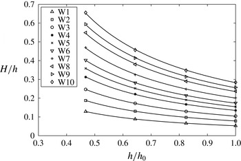

Figure 12. The shoaling rate exponent, $n$
, calculated from a power law fit to the data, (4.1), as a function of the incident wave nonlinearity. The vertical bars represent the uncertainty in
$n$
, calculated from a power law fit to the data, (4.1), as a function of the incident wave nonlinearity. The vertical bars represent the uncertainty in $n$
(see the discussion in the text).
$n$
(see the discussion in the text).
The three wave gauges on the slope and the wave gauge at the toe provide wave height data for $0.47<h/h_{0}<1$
. The data from repeated waves are averaged and fitted to a power law of the form
$0.47<h/h_{0}<1$
. The data from repeated waves are averaged and fitted to a power law of the form
 $$\begin{eqnarray}H\propto h^{n}\end{eqnarray}$$
and plotted in figure 11. The exponent of the power law, $n$
, is plotted in figure 12 as a function of the incident wave height. The uncertainty in the exponent,
$n$
, is plotted in figure 12 as a function of the incident wave height. The uncertainty in the exponent, $n$
, is found by applying the bootstrap technique (Efron & Tibshirani Reference Efron and Tibshirani1993) to the power law fit. The data show that for waves W4 to W10, covering a wide range of incident wave heights,
$n$
, is found by applying the bootstrap technique (Efron & Tibshirani Reference Efron and Tibshirani1993) to the power law fit. The data show that for waves W4 to W10, covering a wide range of incident wave heights, $0.13<{\it\epsilon}_{0}<0.29$
, the shoaling rate hardly changes,
$0.13<{\it\epsilon}_{0}<0.29$
, the shoaling rate hardly changes, $-0.12<n<-0.10$
. Considering all waves, the absolute value of the shoaling rate decreases with increasing incident wave height, but for this slope, there seems to be a limit of approximately
$-0.12<n<-0.10$
. Considering all waves, the absolute value of the shoaling rate decreases with increasing incident wave height, but for this slope, there seems to be a limit of approximately $n=-0.1$
for how slowly the wave height grows. For the smallest incident waves, the rate of shoaling seems to approach that of Green’s law (
$n=-0.1$
for how slowly the wave height grows. For the smallest incident waves, the rate of shoaling seems to approach that of Green’s law ( $n=-0.25$
), but it is still lower in absolute value. The current shoaling data are consistent with the conclusions drawn in the literature: (i) the shoaling of a solitary wave is independent of the incident wave height for large incident wave amplitudes; (ii) when the nonlinearity of the wave remains small, the shoaling rate near the toe is closer to Green’s law. The current experiments do not show evidence of the two zones of shoaling, although Li & Raichlen (Reference Li and Raichlen1998) point out that on steeper slopes, the waves tend to break before they have a chance to evolve due to the effect of the slope.
$n=-0.25$
), but it is still lower in absolute value. The current shoaling data are consistent with the conclusions drawn in the literature: (i) the shoaling of a solitary wave is independent of the incident wave height for large incident wave amplitudes; (ii) when the nonlinearity of the wave remains small, the shoaling rate near the toe is closer to Green’s law. The current experiments do not show evidence of the two zones of shoaling, although Li & Raichlen (Reference Li and Raichlen1998) point out that on steeper slopes, the waves tend to break before they have a chance to evolve due to the effect of the slope.
4.3. Wave breaking and collapse
In the current study, two types of breakers were observed: surging breakers and plunging breakers (see table 1). For plunging breakers, the overturning crest formed a jet that hit the dry land onshore of the stillwater shoreline, and for surging breakers, the front face of the wave became very steep as it moved past the stillwater shoreline and then collapsed.
The breaking point is usually defined as the location at which some part of the free surface becomes vertical, corresponding to the mathematical interpretation of breaking that leads to the theoretical breaking criteria, (2.7) and (2.8). Since there was no opportunity to observe the waves from the side in these experiments to gather data on instantaneous wave shape, it was not possible to locate the breaking points. Whether wave breaking occurred was decided by whether the surface of the water remained smooth and free of entrained air during the uprush, which could be determined from the overhead camera data. If the wave broke, the location onshore of the stillwater shoreline at which the surface of the water was no longer smooth was identified by the overhead camera data and is called the collapse point in this study to distinguish it from the breaking point and because of the process of rapid conversion of potential energy to kinetic energy, analogous to bore collapse, that followed. The collapse points for all breaking waves fall within a narrow region onshore of the stillwater shoreline $0.1<x<0.3$
m as seen in figure 5, which also shows that surging breakers collapsed further onshore than plunging breakers. The time at which this collapse point occurs is referred to as the collapse time and is given in table 2.
$0.1<x<0.3$
m as seen in figure 5, which also shows that surging breakers collapsed further onshore than plunging breakers. The time at which this collapse point occurs is referred to as the collapse time and is given in table 2.
Table 2. Nearshore and swash properties of solitary waves. (i) The collapse time for all breaking waves. (ii) Local properties of all solitary waves at location L2 ( $h=0.10$
m,
$h=0.10$
m, $h/h_{0}=0.058$
):
$h/h_{0}=0.058$
): $H_{L2}$
,
$H_{L2}$
, $(H/h)_{L2}$
,
$(H/h)_{L2}$
, $M_{L2}$
. (iii) Predicted and measured swash initiation shoreline velocities:
$M_{L2}$
. (iii) Predicted and measured swash initiation shoreline velocities: $U_{s,p}$
,
$U_{s,p}$
, $U_{s}$
. (iv) Constant value of the characteristic variable,
$U_{s}$
. (iv) Constant value of the characteristic variable, ${\it\alpha}$
, as determined from measurements in the swash:
${\it\alpha}$
, as determined from measurements in the swash: $U_{{\it\alpha},(x>0)}$
. (v) Measured maximum downrush velocity and Froude number at location L2:
$U_{{\it\alpha},(x>0)}$
. (v) Measured maximum downrush velocity and Froude number at location L2: $U_{d,L2}$
,
$U_{d,L2}$
, $\mathit{Fr}_{d,L2}$
.
$\mathit{Fr}_{d,L2}$
.

According to the breaking criterion provided in Synolakis (Reference Synolakis1987), all waves with ${\it\epsilon}_{0}>0.0517$
would break during uprush, whereas waves up to
${\it\epsilon}_{0}>0.0517$
would break during uprush, whereas waves up to ${\it\epsilon}_{0}=0.1$
were observed to show no signs of breaking. This underestimation in the wave amplitude required for breaking is probably due to the shallow water approximation made in that theory which neglects the effects of dispersion, which act against wave steepening and may locally alter whether the free surface becomes vertical. The Synolakis (Reference Synolakis1987) theory is also restricted to incident solitary waves of very low nonlinearity (
${\it\epsilon}_{0}=0.1$
were observed to show no signs of breaking. This underestimation in the wave amplitude required for breaking is probably due to the shallow water approximation made in that theory which neglects the effects of dispersion, which act against wave steepening and may locally alter whether the free surface becomes vertical. The Synolakis (Reference Synolakis1987) theory is also restricted to incident solitary waves of very low nonlinearity ( ${\it\epsilon}_{0}\ll 1$
), and thus the theory may be inappropriate for the larger-amplitude solitary waves used in this study. On the other hand, visual observations confirmed that the type of breaking event that occurred matched the prediction of the slope parameter,
${\it\epsilon}_{0}\ll 1$
), and thus the theory may be inappropriate for the larger-amplitude solitary waves used in this study. On the other hand, visual observations confirmed that the type of breaking event that occurred matched the prediction of the slope parameter, $S_{0}$
, defined in (2.16), that was formed using data from numerical computations of the fully nonlinear potential flow equations by Grilli et al. (Reference Grilli, Svendsen and Subramanya1997). In the following sections, we present our results, taken from a single slope, in terms of
$S_{0}$
, defined in (2.16), that was formed using data from numerical computations of the fully nonlinear potential flow equations by Grilli et al. (Reference Grilli, Svendsen and Subramanya1997). In the following sections, we present our results, taken from a single slope, in terms of $S_{0}$
, so that properties of the swash can be studied in terms of the breaker type and future results on different slopes can be more meaningfully compared with the present results.
$S_{0}$
, so that properties of the swash can be studied in terms of the breaker type and future results on different slopes can be more meaningfully compared with the present results.
4.4. Shoreline motion
The tracked shoreline position along the slope, $x_{s}(t)$
, for all waves is plotted in figure 13. A second-order accurate finite difference scheme was used to obtain the shoreline velocity along the slope,
$x_{s}(t)$
, for all waves is plotted in figure 13. A second-order accurate finite difference scheme was used to obtain the shoreline velocity along the slope, $u_{s}(t)$
. Figure 14 shows the shoreline velocity as a function of its position for the three non-breaking waves, two surging breakers and two plunging breakers. For waves that break, the shoreline motion tracking starts when it is already moving with a large velocity immediately following the collapse point, when the water surface first becomes rough. Just prior to that, during the breaking process, the shoreline position is undefined as the wave crest curls over the stillwater shoreline. The shoreline accelerations seen in the initial stages of the surging and plunging breakers are caused by the steepness of the wavefront (a pressure gradient that is favourable in the onshore direction), which is lost when the collapse is completed. A similar feature was observed in the numerical study of Hibberd & Peregrine (Reference Hibberd and Peregrine1979). For the plunging breakers, the collapse point occurs just after the stillwater shoreline, so that the shoreline shows a very short acceleration phase during this time. For the surging breakers, the collapse point occurs further onshore (see figure 5) and thus the shoreline acceleration persists for slightly longer. For non-breaking waves, the shoreline accelerates more gradually from rest at the stillwater shoreline and reaches a maximum velocity before a gradual deceleration until the run-up is reached.
$u_{s}(t)$
. Figure 14 shows the shoreline velocity as a function of its position for the three non-breaking waves, two surging breakers and two plunging breakers. For waves that break, the shoreline motion tracking starts when it is already moving with a large velocity immediately following the collapse point, when the water surface first becomes rough. Just prior to that, during the breaking process, the shoreline position is undefined as the wave crest curls over the stillwater shoreline. The shoreline accelerations seen in the initial stages of the surging and plunging breakers are caused by the steepness of the wavefront (a pressure gradient that is favourable in the onshore direction), which is lost when the collapse is completed. A similar feature was observed in the numerical study of Hibberd & Peregrine (Reference Hibberd and Peregrine1979). For the plunging breakers, the collapse point occurs just after the stillwater shoreline, so that the shoreline shows a very short acceleration phase during this time. For the surging breakers, the collapse point occurs further onshore (see figure 5) and thus the shoreline acceleration persists for slightly longer. For non-breaking waves, the shoreline accelerates more gradually from rest at the stillwater shoreline and reaches a maximum velocity before a gradual deceleration until the run-up is reached.

Figure 13. Shoreline position, $x_{s}(t)$
, for all waves: W1–3, NB; W4–6, SU; W7–10, PL.
$x_{s}(t)$
, for all waves: W1–3, NB; W4–6, SU; W7–10, PL.

Figure 14. Shoreline velocity, $u_{s}(t)$
, for W1–5, W9, W10; waves W6–8 are left off for reasons of space: W1–3, NB; W4–6, SU; W7–10, PL.
$u_{s}(t)$
, for W1–5, W9, W10; waves W6–8 are left off for reasons of space: W1–3, NB; W4–6, SU; W7–10, PL.
The shoreline velocity of the plunging breakers, e.g. W9 and W10 in figure 14, shows a sudden increase near $x=11$
m before falling to zero at the end of the run-up. This feature was also observed by Yeh et al. (Reference Yeh, Ghazali and Marton1989) and Zhang & Liu (Reference Zhang and Liu2008), who called it a ‘mini-collapse’. Zhang & Liu (Reference Zhang and Liu2008) examined the velocity field in the vicinity of the mini-collpase and showed that there was a build-up of fluid behind the swash tip due to the effects of bed friction at the swash tip. The built-up fluid resembled a small bore that created a mini-collapse when it caught up with the shoreline.
$x=11$
m before falling to zero at the end of the run-up. This feature was also observed by Yeh et al. (Reference Yeh, Ghazali and Marton1989) and Zhang & Liu (Reference Zhang and Liu2008), who called it a ‘mini-collapse’. Zhang & Liu (Reference Zhang and Liu2008) examined the velocity field in the vicinity of the mini-collpase and showed that there was a build-up of fluid behind the swash tip due to the effects of bed friction at the swash tip. The built-up fluid resembled a small bore that created a mini-collapse when it caught up with the shoreline.
4.5. Swash initiation shoreline velocity
Figure 15 shows that the wave fronts are very steep for waves W5–10 at location L2 (stillwater depth $h=0.10$
m), although the waves still have smooth rounded crests. These features show sufficient nonlinear steepening to make use of the NSWEs, (2.5), appropriate. The steep fronts can be treated as bore fronts in the context of (2.5) and the wave heights at location L2 as the height of the bores. If the bore strength is high enough, we expect bore evolution to be governed by Whitham’s formula, (2.11), as the bore approaches the stillwater shoreline. Then, the swash initiation shoreline velocity,
$h=0.10$
m), although the waves still have smooth rounded crests. These features show sufficient nonlinear steepening to make use of the NSWEs, (2.5), appropriate. The steep fronts can be treated as bore fronts in the context of (2.5) and the wave heights at location L2 as the height of the bores. If the bore strength is high enough, we expect bore evolution to be governed by Whitham’s formula, (2.11), as the bore approaches the stillwater shoreline. Then, the swash initiation shoreline velocity, $U_{s}$
, is expected to be well predicted by the solution to Whitham’s formula, (2.12), in which the bore height at location L2 provides the initial condition. Table 2 lists the values of the swash initiation shoreline velocity (i) predicted using Whitham’s formula,
$U_{s}$
, is expected to be well predicted by the solution to Whitham’s formula, (2.12), in which the bore height at location L2 provides the initial condition. Table 2 lists the values of the swash initiation shoreline velocity (i) predicted using Whitham’s formula, $U_{s,p}$
, and (ii) measured immediately after collapse,
$U_{s,p}$
, and (ii) measured immediately after collapse, $U_{s}$
.
$U_{s}$
.

Figure 15. The free-surface elevation, ${\it\eta}$
, of waves W5–10 at location L2 (
${\it\eta}$
, of waves W5–10 at location L2 ( $x=-1.21$
m): (a,c,e) W5–7; (b,d,f) W8–10.
$x=-1.21$
m): (a,c,e) W5–7; (b,d,f) W8–10.
Figure 16 plots these predicted and measured swash initiation shoreline velocities, made dimensionless by the offshore linear long-wave speed. The measured maximum shoreline velocity during uprush, $U_{s,m}$
, is also plotted for comparison. There are two sources of uncertainty in the measurement of the shoreline velocity: the truncation error in the finite difference scheme to calculate the shoreline velocity from the shoreline position data and the uncertainty in the position of the shoreline at each datapoint. The uncertainty in the shoreline position dominates in this case, and it is propagated to an uncertainty in the shoreline velocity to give the error bars in the measured swash initiation shoreline velocity (e.g. Taylor Reference Taylor1997). The overall agreement between the predicted and measured values of the swash initiation shoreline velocity verifies the theory of Ho & Meyer (Reference Ho and Meyer1962), who showed that the evolution of the bore during collapse is only very weakly influenced by the details of the bore. However, it can be seen that while the predicted values for the swash initiation shoreline velocity match the measured values very well for plunging breakers (
$U_{s,m}$
, is also plotted for comparison. There are two sources of uncertainty in the measurement of the shoreline velocity: the truncation error in the finite difference scheme to calculate the shoreline velocity from the shoreline position data and the uncertainty in the position of the shoreline at each datapoint. The uncertainty in the shoreline position dominates in this case, and it is propagated to an uncertainty in the shoreline velocity to give the error bars in the measured swash initiation shoreline velocity (e.g. Taylor Reference Taylor1997). The overall agreement between the predicted and measured values of the swash initiation shoreline velocity verifies the theory of Ho & Meyer (Reference Ho and Meyer1962), who showed that the evolution of the bore during collapse is only very weakly influenced by the details of the bore. However, it can be seen that while the predicted values for the swash initiation shoreline velocity match the measured values very well for plunging breakers ( $0.025<S_{0}<0.3$
), the measured values for surging breakers (
$0.025<S_{0}<0.3$
), the measured values for surging breakers ( $0.3<S_{0}<0.37$
) are slightly lower than those predicted. The source of this discrepancy for surging breakers is probably the fact that surging breakers do not completely collapse by the time the shoreline starts to move. We return to this idea in the following section in the context of the flow evolution in the swash.
$0.3<S_{0}<0.37$
) are slightly lower than those predicted. The source of this discrepancy for surging breakers is probably the fact that surging breakers do not completely collapse by the time the shoreline starts to move. We return to this idea in the following section in the context of the flow evolution in the swash.
A similar agreement in the predicted and measured swash initiation shoreline velocities was also observed by Yeh et al. (Reference Yeh, Ghazali and Marton1989), who found that for undular bores (or weak bores), the swash initiation shoreline velocity predicted by Whitham’s formula matched the measured value, but it occurred slightly onshore of the stillwater shoreline. The description of the collapse of undular bores matches that of the plunging breakers in this study, i.e. the collapse occurs via overturning of the fluid onto the dry land onshore of the stillwater shoreline. For fully developed bores (or strong bores), Yeh et al. (Reference Yeh, Ghazali and Marton1989) found that the bore exchanges momentum with the wedge-shaped fluid in front of the bore and pushes this fluid onshore to initiate the swash. This momentum exchange causes a lower initial shoreline velocity than predicted by Whitham’s formula. Such a transition might be expected for solitary waves that are spilling breakers.

Figure 16. Swash initiation shoreline velocity – comparison of predictions and measurements: ○, $U_{s,p}$
;
$U_{s,p}$
; $\times$
,
$\times$
, $U_{s}$
; ◃,
$U_{s}$
; ◃, $U_{s,m}$
. The error bars represent the uncertainty in the measurement of the shoreline velocity (see the discussion in the text) and are not shown for the maximum measured shoreline velocity,
$U_{s,m}$
. The error bars represent the uncertainty in the measurement of the shoreline velocity (see the discussion in the text) and are not shown for the maximum measured shoreline velocity, $U_{s,m}$
, for reasons of space.
$U_{s,m}$
, for reasons of space.
Figure 16 also shows that the dimensionless swash initiation shoreline velocity for solitary waves that barely break ( $S_{0}\approx 0.35$
) is close to the offshore linear long-wave speed,
$S_{0}\approx 0.35$
) is close to the offshore linear long-wave speed, $\sqrt{gh_{0}}$
. As
$\sqrt{gh_{0}}$
. As $S_{0}$
decreases towards plunging breakers,
$S_{0}$
decreases towards plunging breakers, $U_{s}$
increases to approximately
$U_{s}$
increases to approximately $1.6\sqrt{gh_{0}}$
, and it may increase further for even larger waves. Overall, the relationship between
$1.6\sqrt{gh_{0}}$
, and it may increase further for even larger waves. Overall, the relationship between $U_{s}/\sqrt{gh_{0}}$
and
$U_{s}/\sqrt{gh_{0}}$
and $S_{0}$
provides a link between the velocity scale of the swash, i.e. the swash initiation shoreline velocity, and the offshore water depth by using
$S_{0}$
provides a link between the velocity scale of the swash, i.e. the swash initiation shoreline velocity, and the offshore water depth by using $S_{0}$
to predict the breaker type. The data provided here are only for one slope and, in general, there may be an additional slope dependence since the slope is of primary importance in the determination of increases in wave height during shoaling.
$S_{0}$
to predict the breaker type. The data provided here are only for one slope and, in general, there may be an additional slope dependence since the slope is of primary importance in the determination of increases in wave height during shoaling.
4.6. Flow evolution in the swash
The time series of a typical set of results for the free-surface elevation, near-bed velocity and bed shear stress in the swash measurement zone are plotted in figure 17. For a given location onshore of the collapse point, the bed shear stress is highest (and directed onshore) at the swash tip when the shoreline arrives, and the bed shear stress values are high (but directed offshore) near the end of the downrush. Further discussion of the bed shear stress is left to the following section, but at this point it is important to note that during the mid-swash duration, after the swash tip passes and before the end of the downrush, the bed shear stress is small and velocity data are available from the ADV (as mentioned is § 3.1, the ADV velocity measurements are only available for a truncated time during the swash when the SNR is above a threshold value).

Figure 17. Free-surface elevation, near-bed velocity and bed shear stress for wave W10 (PL, $H_{0}=0.493$
m,
$H_{0}=0.493$
m, ${\it\epsilon}_{0}=0.286$
) at location L5 (
${\it\epsilon}_{0}=0.286$
) at location L5 ( $x=2.42$
m). (a) Free-surface elevation,
$x=2.42$
m). (a) Free-surface elevation, ${\it\eta}$
. (b) Near-bed velocity,
${\it\eta}$
. (b) Near-bed velocity, $u$
. (c) Bed shear stress,
$u$
. (c) Bed shear stress, ${\it\tau}_{b}$
.
${\it\tau}_{b}$
.
Given that the applicability of the bore collapse theory to breaking solitary waves was affirmed in § 4.5 and bed friction is found to be significant only in the swash tip and at the end of the downrush, it is natural to ask whether the flow evolution in the mid-swash duration follows the swash solution, (2.14), since it was established in § 2.2.3 that bore collapse provides a valid initial condition for the swash solution. Figure 18 plots the characteristic variable, ${\it\alpha}$
, as a function of time for all breaking waves (W4–10). The value of
${\it\alpha}$
, as a function of time for all breaking waves (W4–10). The value of ${\it\alpha}=\overline{u}+2c+gst_{s}$
is calculated from measurements: the free-surface elevation is used to compute the local long-wave celerity,
${\it\alpha}=\overline{u}+2c+gst_{s}$
is calculated from measurements: the free-surface elevation is used to compute the local long-wave celerity, $c=\sqrt{g{\it\eta}}$
, the near-bed velocity,
$c=\sqrt{g{\it\eta}}$
, the near-bed velocity, $u$
, is assumed to approximate the depth-averaged velocity,
$u$
, is assumed to approximate the depth-averaged velocity, $\overline{u}$
, during the mid-swash duration (vertical variation of the horizontal velocity is weak in the swash, e.g. Pedersen et al.
Reference Pedersen, Lindstrom, Bertelsen, Jensen, Laskovski and Sælevik2013) and the collapse point as described in § 4.3 is taken to be
$\overline{u}$
, during the mid-swash duration (vertical variation of the horizontal velocity is weak in the swash, e.g. Pedersen et al.
Reference Pedersen, Lindstrom, Bertelsen, Jensen, Laskovski and Sælevik2013) and the collapse point as described in § 4.3 is taken to be $(x,t_{s})=(0,0)$
. Additionally, the value of
$(x,t_{s})=(0,0)$
. Additionally, the value of ${\it\alpha}$
is averaged across all measurement locations onshore of the stillwater shoreline (L3–L9) because
${\it\alpha}$
is averaged across all measurement locations onshore of the stillwater shoreline (L3–L9) because ${\it\alpha}$
does not vary appreciably in
${\it\alpha}$
does not vary appreciably in $x$
. The data in figure 18 show that
$x$
. The data in figure 18 show that ${\it\alpha}\approx \text{const.}$
throughout the swash flow, except near the swash tip and towards the end of the downrush where the effects of vertical accelerations or bed friction may be important locally. A constant
${\it\alpha}\approx \text{const.}$
throughout the swash flow, except near the swash tip and towards the end of the downrush where the effects of vertical accelerations or bed friction may be important locally. A constant ${\it\alpha}$
is in accordance with the swash solution, but unlike the swash solution, the data in figure 18 show that the constant is not necessarily equal to the measured swash initiation shoreline velocity,
${\it\alpha}$
is in accordance with the swash solution, but unlike the swash solution, the data in figure 18 show that the constant is not necessarily equal to the measured swash initiation shoreline velocity, $U_{s}$
. By taking a time average of the data in figure 18 during the mid-swash duration, the constant value of
$U_{s}$
. By taking a time average of the data in figure 18 during the mid-swash duration, the constant value of ${\it\alpha}$
in the swash is calculated. This constant value is denoted as
${\it\alpha}$
in the swash is calculated. This constant value is denoted as $U_{{\it\alpha},(x>0)}$
and is listed in table 2 for all breaking waves (W4–10). Figures 19 and 20 plot the free-surface elevation and the near-bed velocity for two breaking waves (W5, W8) at two separate locations (L5, L8) and compare the data with the swash solution, (2.14), which is calculated using
$U_{{\it\alpha},(x>0)}$
and is listed in table 2 for all breaking waves (W4–10). Figures 19 and 20 plot the free-surface elevation and the near-bed velocity for two breaking waves (W5, W8) at two separate locations (L5, L8) and compare the data with the swash solution, (2.14), which is calculated using $U_{{\it\alpha},(x>0)}$
instead of the measured
$U_{{\it\alpha},(x>0)}$
instead of the measured $U_{s}$
. The data match the swash solution very well, as expected since the value of
$U_{s}$
. The data match the swash solution very well, as expected since the value of $U_{{\it\alpha},(x>0)}$
was determined from the data. However, the more meaningful result is that the flow evolution in the swash for breaking solitary waves does follow the swash solution, since
$U_{{\it\alpha},(x>0)}$
was determined from the data. However, the more meaningful result is that the flow evolution in the swash for breaking solitary waves does follow the swash solution, since ${\it\alpha}\approx \text{const.}$
, but the constant, which is also the only free parameter in the swash solution, must be correctly scaled. Then, important quantities such as the maximum flow depth and time of flow reversal at a given location can be accurately determined. With the knowledge that the flow evolution of the swash of breaking solitary waves follows the swash solution, the following salient features of this flow can be pointed out. The time of flow reversal does not necessarily occur in phase with the maximum flow depth – the free surface starts to decrease while the velocity is still positive. Flow reversal occurs earlier further down the slope, and the location where flow reversal occurs climbs the slope, stretching and thinning the swash flow. The free-surface gradient,
${\it\alpha}\approx \text{const.}$
, but the constant, which is also the only free parameter in the swash solution, must be correctly scaled. Then, important quantities such as the maximum flow depth and time of flow reversal at a given location can be accurately determined. With the knowledge that the flow evolution of the swash of breaking solitary waves follows the swash solution, the following salient features of this flow can be pointed out. The time of flow reversal does not necessarily occur in phase with the maximum flow depth – the free surface starts to decrease while the velocity is still positive. Flow reversal occurs earlier further down the slope, and the location where flow reversal occurs climbs the slope, stretching and thinning the swash flow. The free-surface gradient, $\partial {\it\eta}/\partial x$
, is positive, or equivalently the total fluid particle acceleration is negative, for the majority of the swash. These features are discussed in more detail in the context of field measurements by Baldock & Hughes (Reference Baldock and Hughes2006).
$\partial {\it\eta}/\partial x$
, is positive, or equivalently the total fluid particle acceleration is negative, for the majority of the swash. These features are discussed in more detail in the context of field measurements by Baldock & Hughes (Reference Baldock and Hughes2006).

Figure 18. The characteristic variable, ${\it\alpha}$
, calculated from experimental data and made dimensionless by the measured swash initiation shoreline velocity,
${\it\alpha}$
, calculated from experimental data and made dimensionless by the measured swash initiation shoreline velocity, $U_{s}$
, as a function of time for all breaking waves, W4–10. The origin of time for the swash of breaking waves,
$U_{s}$
, as a function of time for all breaking waves, W4–10. The origin of time for the swash of breaking waves, $t_{s}=0$
, is the collapse time given in table 2.
$t_{s}=0$
, is the collapse time given in table 2.

Figure 19. Free-surface elevation, ${\it\eta}$
, and near-bed velocity,
${\it\eta}$
, and near-bed velocity, $u$
, for W5 (SU,
$u$
, for W5 (SU, $H_{0}=0.261$
m,
$H_{0}=0.261$
m, ${\it\epsilon}_{0}=0.151$
) at locations L5 (
${\it\epsilon}_{0}=0.151$
) at locations L5 ( $x=2.42$
m) and L8 (
$x=2.42$
m) and L8 ( $x=6.10$
m), and comparisons with the swash solution, (2.14), scaled using
$x=6.10$
m), and comparisons with the swash solution, (2.14), scaled using $U_{{\it\alpha},(x>0)}$
: (a) ——,
$U_{{\it\alpha},(x>0)}$
: (a) ——, ${\it\eta}$
at L5; ——,
${\it\eta}$
at L5; ——, ${\it\eta}$
at L8; — —,
${\it\eta}$
at L8; — —, ${\it\eta}$
from the swash solution, (2.14); (b) ——,
${\it\eta}$
from the swash solution, (2.14); (b) ——, $u$
at L5; ——,
$u$
at L5; ——, $u$
at L8; — —,
$u$
at L8; — —, $u$
from the swash solution, (2.14); ○, shoreline velocity,
$u$
from the swash solution, (2.14); ○, shoreline velocity, $u_{s}$
, at L5; ●, shoreline velocity,
$u_{s}$
, at L5; ●, shoreline velocity, $u_{s}$
, at L8. The origin of time for the swash of breaking waves,
$u_{s}$
, at L8. The origin of time for the swash of breaking waves, $t_{s}=0$
, is the collapse time given in table 2.
$t_{s}=0$
, is the collapse time given in table 2.

Figure 20. Free-surface elevation, ${\it\eta}$
, and near-bed velocity,
${\it\eta}$
, and near-bed velocity, $u$
, for W8 (PL,
$u$
, for W8 (PL, $H_{0}=0.410$
m,
$H_{0}=0.410$
m, ${\it\epsilon}_{0}=0.237$
) at locations L5 (
${\it\epsilon}_{0}=0.237$
) at locations L5 ( $x=2.42$
m) and L8 (
$x=2.42$
m) and L8 ( $x=6.10$
m), and comparisons with the swash solution, (2.14), scaled using
$x=6.10$
m), and comparisons with the swash solution, (2.14), scaled using $U_{{\it\alpha},(x>0)}$
: (a) ——,
$U_{{\it\alpha},(x>0)}$
: (a) ——, ${\it\eta}$
at L5; ——,
${\it\eta}$
at L5; ——, ${\it\eta}$
at L8; — —,
${\it\eta}$
at L8; — —, ${\it\eta}$
from the swash solution, (2.14); (b) ——,
${\it\eta}$
from the swash solution, (2.14); (b) ——, $u$
at L5; ——,
$u$
at L5; ——, $u$
at L8; — —,
$u$
at L8; — —, $u$
from the swash solution, (2.14); ○, shoreline velocity,
$u$
from the swash solution, (2.14); ○, shoreline velocity, $u_{s}$
, at L5; ●, shoreline velocity,
$u_{s}$
, at L5; ●, shoreline velocity, $u_{s}$
, at L8. The origin of time for the swash of breaking waves,
$u_{s}$
, at L8. The origin of time for the swash of breaking waves, $t_{s}=0$
, is the collapse time given in table 2.
$t_{s}=0$
, is the collapse time given in table 2.

Figure 21. Comparisons of different estimates for the swash initiation shoreline velocity: ○, $U_{s,p}$
, predicted from Whitham’s formula for bore collapse, (2.11)–(2.12);
$U_{s,p}$
, predicted from Whitham’s formula for bore collapse, (2.11)–(2.12); $\times$
,
$\times$
, $U_{s}$
, measured initial shoreline velocity with error bars representing uncertainty (same as figure 16); ●,
$U_{s}$
, measured initial shoreline velocity with error bars representing uncertainty (same as figure 16); ●, $U_{{\it\alpha},(x>0)}$
, constant value of the characteristic variable,
$U_{{\it\alpha},(x>0)}$
, constant value of the characteristic variable, ${\it\alpha}$
, from measurements in the swash.
${\it\alpha}$
, from measurements in the swash.
To compare the various estimates and measurements of the swash initiation shoreline velocity, figure 21 plots the direct measurement of the initial shoreline velocity, $U_{s}$
, the prediction of the swash initiation shoreline velocity from wave height measurements at location L2,
$U_{s}$
, the prediction of the swash initiation shoreline velocity from wave height measurements at location L2, $U_{s,p}$
, and the constant value of the characteristic variable,
$U_{s,p}$
, and the constant value of the characteristic variable, ${\it\alpha}$
, determined from measurements in the swash,
${\it\alpha}$
, determined from measurements in the swash, $U_{{\it\alpha},(x>0)}$
, against the slope parameter,
$U_{{\it\alpha},(x>0)}$
, against the slope parameter, $S_{0}$
. As
$S_{0}$
. As $S_{0}$
decreases, i.e. as the breaker type moves from surging to plunging, the relative magnitudes of the three swash initiation shoreline velocity scales change from
$S_{0}$
decreases, i.e. as the breaker type moves from surging to plunging, the relative magnitudes of the three swash initiation shoreline velocity scales change from $U_{{\it\alpha},(x>0)}>U_{s,p}>U_{s}$
to
$U_{{\it\alpha},(x>0)}>U_{s,p}>U_{s}$
to $U_{{\it\alpha},(x>0)}<U_{s,p}<U_{s}$
, although the difference between
$U_{{\it\alpha},(x>0)}<U_{s,p}<U_{s}$
, although the difference between $U_{s}$
and
$U_{s}$
and $U_{s,p}$
is not appreciable for the plunging breakers.
$U_{s,p}$
is not appreciable for the plunging breakers.
For surging breakers, the corresponding physical interpretation is that the flow in the swash zone is driven by a larger initial energy than that predicted by bore collapse theory, which in turn is larger than the energy corresponding to the velocity of the shoreline when it first begins moving. As discussed in § 4.5, the initial shoreline velocity for surging breakers is lower than that predicted by bore collapse theory because the theory assumes that the height of the bore collapses to zero and the conversion between potential energy of the bore and kinetic energy of the swash is complete by the time the shoreline starts to move. Due to the kinematics of surging breakers (see Jensen et al. (Reference Jensen, Pedersen and Wood2003) for detailed measurements of the velocity and acceleration fields near the stillwater shoreline for a surging breaker), this transformation is not complete when the shoreline starts to move. The same idea can also be interpreted as an ambiguity in the location and time of collapse, $(x,t_{s})=(0,0)$
, in the context of bore collapse theory. Additionally, bore collapse theory is valid when the initial bore strength is high, as mentioned in § 2.2.2 and discussed in Ho & Meyer (Reference Ho and Meyer1962). Thus, the prediction from bore collapse theory,
$(x,t_{s})=(0,0)$
, in the context of bore collapse theory. Additionally, bore collapse theory is valid when the initial bore strength is high, as mentioned in § 2.2.2 and discussed in Ho & Meyer (Reference Ho and Meyer1962). Thus, the prediction from bore collapse theory, $U_{s,p}$
, may be an underestimate for surging breakers because, as measured at location L2, they may not be a good approximation to bores of high strength, i.e. their dynamics is not the same as that of a bore of the same height. The milder wave fronts of waves W5–7 compared with waves W8–10 in figure 15 show evidence for this argument. Alternatively, it can be said that for surging breakers, data are required from closer to the stillwater shoreline than location L2 to use bore collapse theory.
$U_{s,p}$
, may be an underestimate for surging breakers because, as measured at location L2, they may not be a good approximation to bores of high strength, i.e. their dynamics is not the same as that of a bore of the same height. The milder wave fronts of waves W5–7 compared with waves W8–10 in figure 15 show evidence for this argument. Alternatively, it can be said that for surging breakers, data are required from closer to the stillwater shoreline than location L2 to use bore collapse theory.
For plunging breakers, $U_{s}\approx U_{s,p}$
to within the uncertainty of measurement, suggesting that bore collapse theory is valid, but
$U_{s}\approx U_{s,p}$
to within the uncertainty of measurement, suggesting that bore collapse theory is valid, but $U_{{\it\alpha},(x>0)}<U_{s}$
. The reason for a swash zone flow that is driven by a lower initial energy than that corresponding to the initial shoreline velocity is probably the loss of energy from the mean flow to turbulent kinetic energy in the violent breaking process that occurs in plunging breakers. Overall, for the range of breaker types investigated, the swash zone flow is driven by an initial energy that corresponds to a swash initiation shoreline velocity in the range
$U_{{\it\alpha},(x>0)}<U_{s}$
. The reason for a swash zone flow that is driven by a lower initial energy than that corresponding to the initial shoreline velocity is probably the loss of energy from the mean flow to turbulent kinetic energy in the violent breaking process that occurs in plunging breakers. Overall, for the range of breaker types investigated, the swash zone flow is driven by an initial energy that corresponds to a swash initiation shoreline velocity in the range $1.1\sqrt{gh_{0}}<U_{{\it\alpha},(x>0)}<1.4\sqrt{gh_{0}}$
.
$1.1\sqrt{gh_{0}}<U_{{\it\alpha},(x>0)}<1.4\sqrt{gh_{0}}$
.
4.7. Bed shear stress
The time series of the bed shear stress and near-bed velocity in the swash measurement zone for three representative locations (L2, L5 and L8) for three representative waves (W3, non-breaking; W5, surging breaker; W10, plunging breaker) are shown in figures 22–24. The sign convention for the bed shear stress is positive when it is directed onshore and negative when it is directed offshore. Oscillations in the bed shear stress are seen at locations L2 and L5 in figures 23 and 24 at times corresponding to the collapse times (see table 2) for waves W5 and W10 respectively. These may be vibration noise in the beach caused by the wave collapse. The shoreline velocities for each wave for locations onshore of the stillwater shoreline (L5, L8) are also plotted in figures 22–24. The free-surface elevation and bed pressure for the same waves at the same locations are shown in figures 25–27. At location L2, none of the waves have reached their breaking point, but at location L5, all waves that break have fully collapsed.

Figure 22. Bed shear stress and near-bed velocity for wave W3 (NB, $H_{0}=0.173$
m,
$H_{0}=0.173$
m, ${\it\epsilon}_{0}=0.100$
): ——, bed shear stress,
${\it\epsilon}_{0}=0.100$
): ——, bed shear stress, ${\it\tau}_{b}$
; ——, near-bed velocity,
${\it\tau}_{b}$
; ——, near-bed velocity, $u$
; ○, shoreline velocity,
$u$
; ○, shoreline velocity, $u_{s}$
. Locations: L2 (
$u_{s}$
. Locations: L2 ( $x=-1.21$
m); L5 (
$x=-1.21$
m); L5 ( $x=2.42$
m); L8 (
$x=2.42$
m); L8 ( $x=6.10$
m).
$x=6.10$
m).

Figure 23. Bed shear stress and near-bed velocity for wave W5 (SU, $H_{0}=0.261$
m,
$H_{0}=0.261$
m, ${\it\epsilon}_{0}=0.151$
): ——, bed shear stress,
${\it\epsilon}_{0}=0.151$
): ——, bed shear stress, ${\it\tau}_{b}$
; ——, near-bed velocity,
${\it\tau}_{b}$
; ——, near-bed velocity, $u$
; ○, shoreline velocity,
$u$
; ○, shoreline velocity, $u_{s}$
. Locations: L2 (
$u_{s}$
. Locations: L2 ( $x=-1.21$
m); L5 (
$x=-1.21$
m); L5 ( $x=2.42$
m); L8 (
$x=2.42$
m); L8 ( $x=6.10$
m).
$x=6.10$
m).

Figure 24. Bed shear stress and near-bed velocity for wave W10 (PL, $H_{0}=0.493$
m,
$H_{0}=0.493$
m, ${\it\epsilon}_{0}=0.286$
): ——, bed shear stress,
${\it\epsilon}_{0}=0.286$
): ——, bed shear stress, ${\it\tau}_{b}$
; ——, near-bed velocity,
${\it\tau}_{b}$
; ——, near-bed velocity, $u$
; ○, shoreline velocity,
$u$
; ○, shoreline velocity, $u_{s}$
. Locations: L2 (
$u_{s}$
. Locations: L2 ( $x=-1.21$
m); L5 (
$x=-1.21$
m); L5 ( $x=2.42$
m); L8 (
$x=2.42$
m); L8 ( $x=6.10$
m).
$x=6.10$
m).
At a location onshore of wave collapse, the highest bed shear stress occurs when the swash tip first arrives during uprush, where the water particle velocity must equal the shoreline velocity (figures 22–24). In the same region, the bed pressure rises faster than the free surface (figures 25–27), implying large vertical accelerations, although quantitative comparisons between the bed pressure and the free-surface elevation at the swash tip are not attempted because the free surface is somewhat ill defined at the swash tip due to a large amount of entrained air that rises to the surface. Furthermore, the spatial resolution of the free-surface elevation measurement is coarser than the bed pressure measurement due to the differences in sensor sizes and principles of operation (see § 3). The high values of bed shear stress at the swash tip are thought to be due to the continually developing boundary layer and bore-generated turbulence from the continuous breaking. Measurements of the velocity near the swash tip have so far proven difficult due to the presence of air bubbles, the highly unsteady nature of the swash tip and its fast translational velocity (e.g. O’Donoghue et al.
Reference O’Donoghue, Pokrajac and Hondebrink2010; Kikkert et al.
Reference Kikkert, O’Donoghue, Pokrajac and Dodd2012), but Pedersen et al. (Reference Pedersen, Lindstrom, Bertelsen, Jensen, Laskovski and Sælevik2013) have measured and computed velocity profiles close to a laminar swash tip in a small-scale laboratory study. Baldock et al. (Reference Baldock, Grayson, Torr and Power2014) have also studied a laminar swash tip by using a highly viscous fluid. They showed that there is flow convergence at the swash tip as the fluid near the surface travels faster than the fluid near the bed and impinges onto the bed, creating high strain rates that lead to high values of the bed shear stress. The impingement of the fluid onto the bed may also explain why the bed pressure is measured to be higher than the hydrostatic pressure. Sumer et al. (Reference Sumer, Sen, Karagali, Ceren, Fredsøe, Sottile, Zilioli and Fuhrman2011) showed similar trends for the bed shear stress in the swash of a plunging solitary wave. They used a hot-film sensor that was $0.5~\text{mm}\times 0.5~\text{mm}$
; the small size of the sensor allowed them to also capture turbulent fluctuations of the bed shear stress. In the swash zone, they showed that the instantaneous bed shear stress at the swash tip could be twice the mean bed shear stress, which they obtained through ensemble averaging. Behind the swash tip, the bed shear stress decays rapidly and the pressure returns to hydrostatic. The low values of the bed shear stress are in phase with the velocity due to the absence of strong pressure gradients, unlike boundary layers under waves in water of constant depth where the bed shear stress leads the velocity (e.g. Nielsen Reference Nielsen1992; Liu et al.
Reference Liu, Park and Cowen2007). The flow in this part of the swash cycle, the mid-swash duration, is essentially a gravity-driven flow that follows the evolution predicted by the swash solution, (2.14), as discussed in the previous section.
$0.5~\text{mm}\times 0.5~\text{mm}$
; the small size of the sensor allowed them to also capture turbulent fluctuations of the bed shear stress. In the swash zone, they showed that the instantaneous bed shear stress at the swash tip could be twice the mean bed shear stress, which they obtained through ensemble averaging. Behind the swash tip, the bed shear stress decays rapidly and the pressure returns to hydrostatic. The low values of the bed shear stress are in phase with the velocity due to the absence of strong pressure gradients, unlike boundary layers under waves in water of constant depth where the bed shear stress leads the velocity (e.g. Nielsen Reference Nielsen1992; Liu et al.
Reference Liu, Park and Cowen2007). The flow in this part of the swash cycle, the mid-swash duration, is essentially a gravity-driven flow that follows the evolution predicted by the swash solution, (2.14), as discussed in the previous section.

Figure 25. Free-surface elevation and bed pressure for wave W3 (NB, $H_{0}=0.173$
m,
$H_{0}=0.173$
m, ${\it\epsilon}_{0}=0.100$
): ——, free-surface elevation,
${\it\epsilon}_{0}=0.100$
): ——, free-surface elevation, ${\it\eta}$
; ——, bed pressure,
${\it\eta}$
; ——, bed pressure, $p_{b}$
. Locations: L2 (
$p_{b}$
. Locations: L2 ( $x=-1.21$
m); L5 (
$x=-1.21$
m); L5 ( $x=2.42$
m); L8 (
$x=2.42$
m); L8 ( $x=6.10$
m).
$x=6.10$
m).

Figure 26. Free-surface elevation and bed pressure for wave W5 (SU, $H_{0}=0.261$
m,
$H_{0}=0.261$
m, ${\it\epsilon}_{0}=0.151$
): ——, free-surface elevation,
${\it\epsilon}_{0}=0.151$
): ——, free-surface elevation, ${\it\eta}$
; ——, bed pressure,
${\it\eta}$
; ——, bed pressure, $p_{b}$
. Locations: L2 (
$p_{b}$
. Locations: L2 ( $x=-1.21$
m); L5 (
$x=-1.21$
m); L5 ( $x=2.42$
m); L8 (
$x=2.42$
m); L8 ( $x=6.10$
m).
$x=6.10$
m).

Figure 27. Free-surface elevation and bed pressure for wave W10 (PL, $H_{0}=0.493$
m,
$H_{0}=0.493$
m, ${\it\epsilon}_{0}=0.286$
): ——, free-surface elevation,
${\it\epsilon}_{0}=0.286$
): ——, free-surface elevation, ${\it\eta}$
; ——, bed pressure,
${\it\eta}$
; ——, bed pressure, $p_{b}$
. Locations: L2 (
$p_{b}$
. Locations: L2 ( $x=-1.21$
m); L5 (
$x=-1.21$
m); L5 ( $x=2.42$
m); L8 (
$x=2.42$
m); L8 ( $x=6.10$
m).
$x=6.10$
m).
Towards the end of the downrush, the bed shear stress values are also high (and directed offshore). The flow velocities during this period are also difficult to measure due to the very shallow depths, but the velocity data before the flow depth becomes too shallow show that the flow is accelerated down the slope by gravity and the magnitude of the bed shear stress increases to slow down the flow while the flow depth continues to reduce. The bed shear stress reaches a peak negative value after which it reduces to zero as the water runs out. The velocity must also reduce to zero as the water runs out, and thus at some intermediate stage, the offshore-directed velocity must reach a maximum magnitude when there is a temporary balance between the gravitational acceleration and the bed shear stress (we expect the streamwise velocity gradient and the streamwise pressure gradient not to be of leading-order importance in the momentum balance). During this period, the bed pressure measurements are also higher than the free-surface elevation measurements, implying the existence of vertical accelerations. Although the flow is very shallow, the free surface must be rising relative to the bed in the flow direction, i.e. $\partial {\it\eta}/\partial x<0$
, because the water depth further onshore of the measurement location reduces to zero earlier than the water depth further offshore of the measurement location. Thus, locally, there may exist some streamline curvature that would explain the non-hydrostatic pressure measurements. At location L5, at approximately
$\partial {\it\eta}/\partial x<0$
, because the water depth further onshore of the measurement location reduces to zero earlier than the water depth further offshore of the measurement location. Thus, locally, there may exist some streamline curvature that would explain the non-hydrostatic pressure measurements. At location L5, at approximately $t\approx 22$
s, there is a sudden increase in the magnitude of the bed shear stress in the negative direction for all waves plotted in figures 22–24. A similar feature is observed for other locations. Sumer et al. (Reference Sumer, Sen, Karagali, Ceren, Fredsøe, Sottile, Zilioli and Fuhrman2011) also identified this feature in their results and, using the ensemble averaging procedure to decompose the bed shear stress into mean and fluctuating components, concluded that this point was where the fluctuating component of the bed shear stress was large. Thus, they indicated that this must be the time when the downrush flow boundary layer becomes turbulent, generating fluctuations in the bed shear stress and causing a sudden increase in its mean magnitude.
$t\approx 22$
s, there is a sudden increase in the magnitude of the bed shear stress in the negative direction for all waves plotted in figures 22–24. A similar feature is observed for other locations. Sumer et al. (Reference Sumer, Sen, Karagali, Ceren, Fredsøe, Sottile, Zilioli and Fuhrman2011) also identified this feature in their results and, using the ensemble averaging procedure to decompose the bed shear stress into mean and fluctuating components, concluded that this point was where the fluctuating component of the bed shear stress was large. Thus, they indicated that this must be the time when the downrush flow boundary layer becomes turbulent, generating fluctuations in the bed shear stress and causing a sudden increase in its mean magnitude.
The flow behaviour near the swash tip and towards the end of downrush is not very well understood, but these are the regions in the swash cycle when the bed shear stress is most significant. However, in the mid-swash duration, the flow is well understood, and to attempt to parameterize the bed shear stress in this part of the flow, a local time-varying friction coefficient and Reynolds number can be calculated using the near-bed velocity, free-surface elevation and bed shear stress signals. The friction coefficient is defined as
 $$\begin{eqnarray}C_{f}^{\prime }=\frac{{\it\tau}_{b}}{\frac{1}{2}{\it\rho}u^{2}},\end{eqnarray}$$
where the prime refers to the fact that it is a local time-varying quantity. The Reynolds number is calculated as
 $$\begin{eqnarray}\mathit{Re}^{\prime }=\frac{u{\it\eta}}{{\it\nu}},\end{eqnarray}$$
where the local water depth, ${\it\eta}$
, is chosen as the relevant length scale and the prime once again refers to the fact that it is a local time-varying quantity. These quantities are plotted in figures 28, 29 and 30 for location L5 for waves W3, W5 and W10 respectively. It can be seen that the friction coefficient is not well defined around the time when the flow changes from uprush to downrush and the velocity goes to zero. Furthermore, values for
${\it\eta}$
, is chosen as the relevant length scale and the prime once again refers to the fact that it is a local time-varying quantity. These quantities are plotted in figures 28, 29 and 30 for location L5 for waves W3, W5 and W10 respectively. It can be seen that the friction coefficient is not well defined around the time when the flow changes from uprush to downrush and the velocity goes to zero. Furthermore, values for $C_{f}^{\prime }$
and
$C_{f}^{\prime }$
and $\mathit{Re}^{\prime }$
are not available near the swash tip and near the end of downrush where velocity data are unavailable. During downrush, the data show that for different incident waves, the values of
$\mathit{Re}^{\prime }$
are not available near the swash tip and near the end of downrush where velocity data are unavailable. During downrush, the data show that for different incident waves, the values of $\mathit{Re}^{\prime }$
fall within the range
$\mathit{Re}^{\prime }$
fall within the range $0.5\times 10^{5}<\mathit{Re}^{\prime }<10^{5}$
with a corresponding range of
$0.5\times 10^{5}<\mathit{Re}^{\prime }<10^{5}$
with a corresponding range of $0.005<C_{f}^{\prime }<0.01$
. Barnes et al. (Reference Barnes, O’Donoghue, Alsina and Baldock2009) conducted a careful investigation of the variation in
$0.005<C_{f}^{\prime }<0.01$
. Barnes et al. (Reference Barnes, O’Donoghue, Alsina and Baldock2009) conducted a careful investigation of the variation in $C_{f}^{\prime }$
with
$C_{f}^{\prime }$
with $\mathit{Re}^{\prime }$
and location within the swash using depth-averaged velocities obtained from an NSWE hydrodynamic model. They found that during uprush,
$\mathit{Re}^{\prime }$
and location within the swash using depth-averaged velocities obtained from an NSWE hydrodynamic model. They found that during uprush, $C_{f}^{\prime }$
tends to decrease with increasing
$C_{f}^{\prime }$
tends to decrease with increasing $\mathit{Re}^{\prime }$
, which is the trend for steady flows, but at locations further up the slope in the swash, the same
$\mathit{Re}^{\prime }$
, which is the trend for steady flows, but at locations further up the slope in the swash, the same $\mathit{Re}^{\prime }$
gives a lower
$\mathit{Re}^{\prime }$
gives a lower $C_{f}^{\prime }$
than at locations further down the slope. During downrush,
$C_{f}^{\prime }$
than at locations further down the slope. During downrush, $C_{f}^{\prime }$
initially decreases with increasing
$C_{f}^{\prime }$
initially decreases with increasing $\mathit{Re}^{\prime }$
and then the trend is reversed during the later stages of downrush. They also compared their data with the Colebrook–White formula for steady turbulent open-channel flow and found that
$\mathit{Re}^{\prime }$
and then the trend is reversed during the later stages of downrush. They also compared their data with the Colebrook–White formula for steady turbulent open-channel flow and found that $C_{f}^{\prime }$
was underpredicted during uprush and overpredicted during downrush. These results have been corroborated by the results of O’Donoghue et al. (Reference O’Donoghue, Pokrajac and Hondebrink2010) and Kikkert et al. (Reference Kikkert, O’Donoghue, Pokrajac and Dodd2012), who used a log-law fitting to estimate the bed shear stress from velocity data obtained from particle image velocimetry measurements in the swash. It should be noted that when using velocity measurements to infer the bed shear stress, it was not possible to obtain bed shear stress values near the swash tip and near the end of downrush. The same conclusions can be drawn from the current data, with the trend of decreasing
$C_{f}^{\prime }$
was underpredicted during uprush and overpredicted during downrush. These results have been corroborated by the results of O’Donoghue et al. (Reference O’Donoghue, Pokrajac and Hondebrink2010) and Kikkert et al. (Reference Kikkert, O’Donoghue, Pokrajac and Dodd2012), who used a log-law fitting to estimate the bed shear stress from velocity data obtained from particle image velocimetry measurements in the swash. It should be noted that when using velocity measurements to infer the bed shear stress, it was not possible to obtain bed shear stress values near the swash tip and near the end of downrush. The same conclusions can be drawn from the current data, with the trend of decreasing $C_{f}^{\prime }$
with increasing
$C_{f}^{\prime }$
with increasing $\mathit{Re}^{\prime }$
during uprush and a mixed dependence of
$\mathit{Re}^{\prime }$
during uprush and a mixed dependence of $C_{f}^{\prime }$
on
$C_{f}^{\prime }$
on $\mathit{Re}^{\prime }$
during downrush visible in figures 28–30. Thus, for the data in this study,
$\mathit{Re}^{\prime }$
during downrush visible in figures 28–30. Thus, for the data in this study, $C_{f}^{\prime }$
is not a universal function of
$C_{f}^{\prime }$
is not a universal function of $\mathit{Re}^{\prime }$
, probably because the swash flow is unsteady.
$\mathit{Re}^{\prime }$
, probably because the swash flow is unsteady.

Figure 28. (a) The free-surface elevation, ${\it\eta}$
,
——, and the near-bed velocity,
${\it\eta}$
,
——, and the near-bed velocity, $u$
, ——. (b) The local time-varying Reynolds number,
$u$
, ——. (b) The local time-varying Reynolds number, $\mathit{Re}^{\prime }$
. (c) The local time-varying friction coefficient,
$\mathit{Re}^{\prime }$
. (c) The local time-varying friction coefficient, $C_{f}^{\prime }$
. Location L5 (
$C_{f}^{\prime }$
. Location L5 ( $x=2.42$
m) for wave W3 (NB,
$x=2.42$
m) for wave W3 (NB, $H_{0}=0.173$
m,
$H_{0}=0.173$
m, ${\it\epsilon}_{0}=0.100$
).
${\it\epsilon}_{0}=0.100$
).

Figure 29. (a) The free-surface elevation, ${\it\eta}$
,
——, and the near-bed velocity,
${\it\eta}$
,
——, and the near-bed velocity, $u$
, ——. (b) The local time-varying Reynolds number,
$u$
, ——. (b) The local time-varying Reynolds number, $\mathit{Re}^{\prime }$
. (c) The local time-varying friction coefficient,
$\mathit{Re}^{\prime }$
. (c) The local time-varying friction coefficient, $C_{f}^{\prime }$
. Location L5 (
$C_{f}^{\prime }$
. Location L5 ( $x=2.42$
m) for wave W5 (SU,
$x=2.42$
m) for wave W5 (SU, $H_{0}=0.261$
m,
$H_{0}=0.261$
m, ${\it\epsilon}_{0}=0.151$
).
${\it\epsilon}_{0}=0.151$
).

Figure 30. (a) The free-surface elevation, ${\it\eta}$
,
——, and the near-bed velocity,
${\it\eta}$
,
——, and the near-bed velocity, $u$
, ——. (b) The local time-varying Reynolds number,
$u$
, ——. (b) The local time-varying Reynolds number, $\mathit{Re}^{\prime }$
. (c) The local time-varying friction coefficient,
$\mathit{Re}^{\prime }$
. (c) The local time-varying friction coefficient, $C_{f}^{\prime }$
. Location L5 (
$C_{f}^{\prime }$
. Location L5 ( $x=2.42$
m) for wave W10 (PL,
$x=2.42$
m) for wave W10 (PL, $H_{0}=0.493$
m,
$H_{0}=0.493$
m, ${\it\epsilon}_{0}=0.286$
).
${\it\epsilon}_{0}=0.286$
).
Instead of parameterizing the time-varying value of the bed shear stress, we choose to focus on parameterizing the maximum magnitudes since these occur when the bed shear stress is much more important to the flow dynamics. The maximum magnitudes of the bed shear stress during uprush and downrush at a given location are denoted as ${\it\tau}_{b,u}$
and
${\it\tau}_{b,u}$
and ${\it\tau}_{b,d}$
respectively. The sign convention is retained so that
${\it\tau}_{b,d}$
respectively. The sign convention is retained so that ${\it\tau}_{b,d}$
is a negative quantity referring to the fact that the downrush stress is offshore-directed. These quantities are shown in figure 31. For the breaking waves, W5 and W10, there is an
${\it\tau}_{b,d}$
is a negative quantity referring to the fact that the downrush stress is offshore-directed. These quantities are shown in figure 31. For the breaking waves, W5 and W10, there is an $O(6)$
-fold and
$O(6)$
-fold and $O(7)$
-fold increase in the maximum uprush bed shear stress across the collapse points respectively. Sumer et al. (Reference Sumer, Sen, Karagali, Ceren, Fredsøe, Sottile, Zilioli and Fuhrman2011) observed a similar increase across breaking for their plunging wave case. This increase is usually attributed to the effects of breaking and collapse, which produce high-velocity turbulent flow at the swash tip. However, the non-breaking wave W3 also shows an
$O(7)$
-fold increase in the maximum uprush bed shear stress across the collapse points respectively. Sumer et al. (Reference Sumer, Sen, Karagali, Ceren, Fredsøe, Sottile, Zilioli and Fuhrman2011) observed a similar increase across breaking for their plunging wave case. This increase is usually attributed to the effects of breaking and collapse, which produce high-velocity turbulent flow at the swash tip. However, the non-breaking wave W3 also shows an $O(6)$
-fold increase in the maximum uprush bed shear stress across the stillwater shoreline, indicating that the swash tip generates a much higher bed shear stress than the wave-induced boundary layer even when there is no breaking. There is also an asymmetry in the swash, with larger values of
$O(6)$
-fold increase in the maximum uprush bed shear stress across the stillwater shoreline, indicating that the swash tip generates a much higher bed shear stress than the wave-induced boundary layer even when there is no breaking. There is also an asymmetry in the swash, with larger values of ${\it\tau}_{b,u}$
than
${\it\tau}_{b,u}$
than ${\it\tau}_{b,d}$
, which has been previously noted by Barnes et al. (Reference Barnes, O’Donoghue, Alsina and Baldock2009) and others. This asymmetry is less pronounced further up the slope.
${\it\tau}_{b,d}$
, which has been previously noted by Barnes et al. (Reference Barnes, O’Donoghue, Alsina and Baldock2009) and others. This asymmetry is less pronounced further up the slope.

Figure 31. Maximum magnitudes of the bed shear stress for W3 (NB, $H_{0}=0.173$
m,
$H_{0}=0.173$
m, ${\it\epsilon}_{0}=0.100$
), W5 (SU,
${\it\epsilon}_{0}=0.100$
), W5 (SU, $H_{0}=0.261$
m,
$H_{0}=0.261$
m, ${\it\epsilon}_{0}=0.151$
) and W10 (PL,
${\it\epsilon}_{0}=0.151$
) and W10 (PL, $H_{0}=0.493$
m,
$H_{0}=0.493$
m, ${\it\epsilon}_{0}=0.286$
) as a function of distance from the stillwater shoreline,
${\it\epsilon}_{0}=0.286$
) as a function of distance from the stillwater shoreline, $x$
.
$x$
.
To compare the values of the maximum magnitudes of the bed shear stress in the uprush and downrush for different breaking waves, the maximum magnitudes of the uprush and downrush bed shear stress need to be made dimensionless. The swash initiation shoreline velocity has been identified as the largest and defining velocity scale of the swash in previous sections, and thus it is the appropriate velocity scale to make the maximum magnitudes of the bed shear stress dimensionless. Thus, a dimensionless measure of the maximum magnitudes of the uprush and downrush shear stress at a given location can be defined as
 $$\begin{eqnarray}\displaystyle \frac{{\it\tau}_{b,u}}{\frac{1}{2}{\it\rho}U_{{\it\alpha},(x>0)}^{2}}, & & \displaystyle\end{eqnarray}$$
 $$\begin{eqnarray}\displaystyle \frac{{\it\tau}_{b,d}}{\frac{1}{2}{\it\rho}U_{{\it\alpha},(x>0)}^{2}}, & & \displaystyle\end{eqnarray}$$ $U_{{\it\alpha},(x>0)}$
, is used. This estimate is used instead of other estimates of the same quantity because it is derived from the data. Figure 32 shows that the dimensionless maximum magnitudes of the bed shear stress for different incident waves collapse under this normalization, giving further confidence in the importance of this velocity scale in the swash. The maximum magnitude for the uprush dimensionless maximum bed shear stress is
$U_{{\it\alpha},(x>0)}$
, is used. This estimate is used instead of other estimates of the same quantity because it is derived from the data. Figure 32 shows that the dimensionless maximum magnitudes of the bed shear stress for different incident waves collapse under this normalization, giving further confidence in the importance of this velocity scale in the swash. The maximum magnitude for the uprush dimensionless maximum bed shear stress is ${\it\tau}_{b}/(0.5{\it\rho}U_{{\it\alpha},(x>0)}^{2})\approx 0.01$
, which occurs just after the collapse region. The maximum magnitude for the downrush dimensionless maximum bed shear stress is
${\it\tau}_{b}/(0.5{\it\rho}U_{{\it\alpha},(x>0)}^{2})\approx 0.01$
, which occurs just after the collapse region. The maximum magnitude for the downrush dimensionless maximum bed shear stress is ${\it\tau}_{b}/(0.5{\it\rho}U_{{\it\alpha},(x>0)}^{2})\approx 0.002$
, which occurs just before the hydraulic jump. The asymmetry of the bed shear stress between the uprush and downrush is also evident in figure 32.
${\it\tau}_{b}/(0.5{\it\rho}U_{{\it\alpha},(x>0)}^{2})\approx 0.002$
, which occurs just before the hydraulic jump. The asymmetry of the bed shear stress between the uprush and downrush is also evident in figure 32.

Figure 32. Dimensionless maximum magnitudes of the bed shear stress for all breaking waves, W4–10, as function of the dimensionless distance from the stillwater shoreline.
4.8. Run-up
There are many studies of the run-up of solitary waves. Most do not consider the effects of bottom friction, turbulent dissipation or the surface tension, and so the variables of interest are reduced to those shown in figure 1. Analytical solutions are available for the run-up of non-breaking solitary waves, (2.6) and (2.9), but only empirical relationships are available for breaking solitary waves (see Li & Raichlen Reference Li and Raichlen2003; Fuhrman & Madsen Reference Fuhrman and Madsen2008; Lo, Park & Liu Reference Lo, Park and Liu2013). For periodic waves, a surf similarity parameter, first introduced by Battjes (Reference Battjes1974), has been used to predict run-up. Mei (Reference Mei1989) showed how the form of the surf similarity parameter for monochromatic waves is consistent with the breaking criterion from the theory of Carrier & Greenspan (Reference Carrier and Greenspan1958), and following this pattern for solitary waves, Lo et al. (Reference Lo, Park and Liu2013) introduced a solitary wave surf parameter, $s(H_{0}/h_{0})^{-9/10}$
, where the breaking criterion from Synolakis (Reference Synolakis1987), (2.7), is reduced to its fundamental form by removing all constants. A similar solitary wave surf parameter, in which the exponent is
$s(H_{0}/h_{0})^{-9/10}$
, where the breaking criterion from Synolakis (Reference Synolakis1987), (2.7), is reduced to its fundamental form by removing all constants. A similar solitary wave surf parameter, in which the exponent is $-1$
instead of
$-1$
instead of $-9/10$
, was introduced by Kobayashi & Karjadi (Reference Kobayashi and Karjadi1994) and given an explicit form by Fuhrman & Madsen (Reference Fuhrman and Madsen2008). Intuitively, for a given offshore water depth and slope of the plane beach, the highest run-up normalized by the incident wave height,
$-9/10$
, was introduced by Kobayashi & Karjadi (Reference Kobayashi and Karjadi1994) and given an explicit form by Fuhrman & Madsen (Reference Fuhrman and Madsen2008). Intuitively, for a given offshore water depth and slope of the plane beach, the highest run-up normalized by the incident wave height, $R/H_{0}$
, should be expected to occur for a solitary wave that almost breaks. The reasoning behind this intuition is that large waves that break far offshore form fully developed bores by the time they reach nearshore, and in doing so they lose energy that would have been converted to potential energy of the run-up. On the other hand, for non-breaking waves, the higher the incident wave height, the larger the incoming energy and the larger the run-up are expected to be. Therefore, it is reasonable to expect that the dimensionless run-up,
$R/H_{0}$
, should be expected to occur for a solitary wave that almost breaks. The reasoning behind this intuition is that large waves that break far offshore form fully developed bores by the time they reach nearshore, and in doing so they lose energy that would have been converted to potential energy of the run-up. On the other hand, for non-breaking waves, the higher the incident wave height, the larger the incoming energy and the larger the run-up are expected to be. Therefore, it is reasonable to expect that the dimensionless run-up, $R/H_{0}$
, should be a function of a breaking criterion. The most reliable parameter to predict solitary wave breaker type is the slope parameter proposed by Grilli et al. (Reference Grilli, Svendsen and Subramanya1997), since it is derived, albeit empirically, from computations of the fully nonlinear potential flow equations on a range of slopes and incident amplitudes. Interestingly, the Synolakis (Reference Synolakis1987) run-up law, (2.6), can be re-expressed using the slope parameter to give
$R/H_{0}$
, should be a function of a breaking criterion. The most reliable parameter to predict solitary wave breaker type is the slope parameter proposed by Grilli et al. (Reference Grilli, Svendsen and Subramanya1997), since it is derived, albeit empirically, from computations of the fully nonlinear potential flow equations on a range of slopes and incident amplitudes. Interestingly, the Synolakis (Reference Synolakis1987) run-up law, (2.6), can be re-expressed using the slope parameter to give
 $$\begin{eqnarray}\frac{R}{H_{0}}=3.49S_{0}^{-1/2},\end{eqnarray}$$
which was also identified by Fuhrman & Madsen (Reference Fuhrman and Madsen2008), who refer to a form of $S_{0}$
without any constants as a solitary wave run-up parameter. It should be noted that, as mentioned in § 2.2.1, the run-up law is only formally valid for
$S_{0}$
without any constants as a solitary wave run-up parameter. It should be noted that, as mentioned in § 2.2.1, the run-up law is only formally valid for $S_{0}\ll 5.28$
. The run-up of solitary waves from current and previous laboratory studies is plotted against the solitary wave slope parameter in figure 33. It can be seen that the highest run-up is in the vicinity of the breaking criterion,
$S_{0}\ll 5.28$
. The run-up of solitary waves from current and previous laboratory studies is plotted against the solitary wave slope parameter in figure 33. It can be seen that the highest run-up is in the vicinity of the breaking criterion, $S_{0}=0.37$
, confirming that
$S_{0}=0.37$
, confirming that $S_{0}$
is a relevant parameter. In fact, if the highest dimensionless run-up is expected from waves that almost break, the data in figure 33 actually suggest that the breaking criterion of Grilli et al. (Reference Grilli, Svendsen and Subramanya1997) slightly overestimates the incident wave amplitude and that waves of a slightly lower incident amplitude are likely to break, so that the breaking criterion should be
$S_{0}$
is a relevant parameter. In fact, if the highest dimensionless run-up is expected from waves that almost break, the data in figure 33 actually suggest that the breaking criterion of Grilli et al. (Reference Grilli, Svendsen and Subramanya1997) slightly overestimates the incident wave amplitude and that waves of a slightly lower incident amplitude are likely to break, so that the breaking criterion should be $S_{0}\approx 0.4{-}0.5$
. Given that the numerical model used by Grilli et al. (Reference Grilli, Svendsen and Subramanya1997) is 2D (thereby excluding any effects of spanwise instabilities) and excludes both viscosity and surface tension (both of which might be important in the early onset of breaking), it seems reasonable to expect that breaking in laboratory experiments starts to happen earlier than predicted by potential flow equations. The data of Hsiao et al. (Reference Hsiao, Hsu, Lin and Chang2008), which were obtained on a slope of
$S_{0}\approx 0.4{-}0.5$
. Given that the numerical model used by Grilli et al. (Reference Grilli, Svendsen and Subramanya1997) is 2D (thereby excluding any effects of spanwise instabilities) and excludes both viscosity and surface tension (both of which might be important in the early onset of breaking), it seems reasonable to expect that breaking in laboratory experiments starts to happen earlier than predicted by potential flow equations. The data of Hsiao et al. (Reference Hsiao, Hsu, Lin and Chang2008), which were obtained on a slope of $s=1/60$
, show the same trend as the rest of the data, where the range of slopes spans
$s=1/60$
, show the same trend as the rest of the data, where the range of slopes spans $1/30\leqslant s\leqslant 1$
. Plotted in this way, the data show that Synolakis’s run-up law, (4.5), provides an upper bound for the run-up of non-breaking waves (as might be expected from a theory that does not consider frictional effects) for values of the slope parameter larger than
$1/30\leqslant s\leqslant 1$
. Plotted in this way, the data show that Synolakis’s run-up law, (4.5), provides an upper bound for the run-up of non-breaking waves (as might be expected from a theory that does not consider frictional effects) for values of the slope parameter larger than $S_{0}\approx 0.54$
. The data of Hall & Watts (Reference Hall and Watts1953) show higher run-ups than (4.5), but it is known that the generation mechanism for their solitary waves was rudimentary and thus the run-up measurements are of limited accuracy. The current data differ somewhat from previous data since they are taken at a much larger scale than typical laboratory measurements. However, they are seen to fit well with the rest of the data. It should be noted that the solitary wave surf parameter introduced by Lo et al. (Reference Lo, Park and Liu2013) also provides a collapse of all the data, including the current data and the data of Hsiao et al. (Reference Hsiao, Hsu, Lin and Chang2008). Here, we show that
$S_{0}\approx 0.54$
. The data of Hall & Watts (Reference Hall and Watts1953) show higher run-ups than (4.5), but it is known that the generation mechanism for their solitary waves was rudimentary and thus the run-up measurements are of limited accuracy. The current data differ somewhat from previous data since they are taken at a much larger scale than typical laboratory measurements. However, they are seen to fit well with the rest of the data. It should be noted that the solitary wave surf parameter introduced by Lo et al. (Reference Lo, Park and Liu2013) also provides a collapse of all the data, including the current data and the data of Hsiao et al. (Reference Hsiao, Hsu, Lin and Chang2008). Here, we show that $S_{0}$
provides a credible parameterization of the run-up as well as the breaker type, and that the two phenomena are invariably linked.
$S_{0}$
provides a credible parameterization of the run-up as well as the breaker type, and that the two phenomena are invariably linked.

Figure 33. Run-up of solitary waves plotted against the slope parameter: LO, Lo et al. (Reference Lo, Park and Liu2013); LR, Li & Raichlen (Reference Li and Raichlen2001, Reference Li and Raichlen2002); SY, Synolakis (Reference Synolakis1987); BR, Briggs et al. (Reference Briggs, Synolakis, Harkins and Green1995); HS, Hsiao et al. (Reference Hsiao, Hsu, Lin and Chang2008); CH, Chang, Hwang & Hwung (Reference Chang, Hwang and Hwung2009); HW, Hall & Watts (Reference Hall and Watts1953); LS, Langsholt (Reference Langsholt1981); JN, Jensen et al. (Reference Jensen, Pedersen and Wood2003); PE, Pedersen et al. (Reference Pedersen, Lindstrom, Bertelsen, Jensen, Laskovski and Sælevik2013); CU, current data; ——, Synolakis (Reference Synolakis1987) run-up law, (4.5); — —, Grilli et al. (Reference Grilli, Svendsen and Subramanya1997) breaking criterion, (2.16).

Figure 34. Shoreline velocity comparison with the ideal inviscid case for waves W5 (SU, $H_{0}=0.261$
m,
$H_{0}=0.261$
m, ${\it\epsilon}_{0}=0.151$
) and W10 (PL,
${\it\epsilon}_{0}=0.151$
) and W10 (PL, $H_{0}=0.493$
m,
$H_{0}=0.493$
m, ${\it\epsilon}_{0}=0.286$
): symbols, data; ——, ideal inviscid shoreline motion that follows the motion described by (2.13).
${\it\epsilon}_{0}=0.286$
): symbols, data; ——, ideal inviscid shoreline motion that follows the motion described by (2.13).
For the current data, the reduction in run-up due to dissipation from bottom friction for breaking waves is briefly considered. The run-up measurements can be used to calculate a hypothetical initial shoreline velocity of an ideal frictionless swash that follows (2.13) but reaches the same run-up as the real case. This hypothetical initial shoreline velocity is given by $\sqrt{2gR}$
. The discrepancy between this velocity and the measured swash initiation shoreline velocity gives the scale of the energy dissipation in the swash tip. The implied assumptions are that the energy dissipation is dominantly from friction at the swash tip and the work done by pressure on the swash tip from behind is negligible. Figure 34 shows the comparisons between an ideal frictionless shoreline velocity and the actual shoreline for a surging breaker, W5, and a plunging breaker, W10. It can be seen that the plunging breaker achieves a shoreline velocity of roughly
$\sqrt{2gR}$
. The discrepancy between this velocity and the measured swash initiation shoreline velocity gives the scale of the energy dissipation in the swash tip. The implied assumptions are that the energy dissipation is dominantly from friction at the swash tip and the work done by pressure on the swash tip from behind is negligible. Figure 34 shows the comparisons between an ideal frictionless shoreline velocity and the actual shoreline for a surging breaker, W5, and a plunging breaker, W10. It can be seen that the plunging breaker achieves a shoreline velocity of roughly $1.4\sqrt{2gR}$
. Since energy is proportional to velocity squared, this shows that only just over
$1.4\sqrt{2gR}$
. Since energy is proportional to velocity squared, this shows that only just over $50\,\%$
of the initial energy of the shoreline is converted to the potential energy of the run-up and the rest is lost to dissipation. For the surging breaker, almost
$50\,\%$
of the initial energy of the shoreline is converted to the potential energy of the run-up and the rest is lost to dissipation. For the surging breaker, almost $90\,\%$
of the initial energy is converted to the potential energy of the run-up.
$90\,\%$
of the initial energy is converted to the potential energy of the run-up.
4.9. Run-down
When the supercritical downrush flow meets the near-quiescent offshore water body, a hydraulic jump is created. This hydraulic jump is sometimes referred to as downrush breaking, due to the similarities it shows to conventional wave breaking during uprush (for a description of its formation, see Hibberd & Peregrine Reference Hibberd and Peregrine1979). The occurrence of the hydraulic jump was identified by the overhead cameras, and the region where it occurred for all waves is shown in figure 5. The criterion from Madsen & Schäffer (Reference Madsen and Schäffer2010), (2.8), predicts that for this slope ( $s=1/12$
), all waves with
$s=1/12$
), all waves with ${\it\epsilon}_{0}>0.0325$
would exhibit downrush breaking. All the waves generated satisfied this criterion and they were all observed to break during downrush and create a hydraulic jump. As mentioned in § 2.2.1, the run-down in the Madsen & Schäffer (Reference Madsen and Schäffer2010) theory is for non-breaking waves, and since all waves in this study showed evidence of a hydraulic jump during downrush, a comparison with the theory cannot be made. For waves where a hydraulic jump does occur, the run-down can be defined as the vertical extent below the stillwater shoreline that the hydraulic jump occurs, and these data are shown in table 1. Unfortunately, a general downrush breaking criterion in terms of
${\it\epsilon}_{0}>0.0325$
would exhibit downrush breaking. All the waves generated satisfied this criterion and they were all observed to break during downrush and create a hydraulic jump. As mentioned in § 2.2.1, the run-down in the Madsen & Schäffer (Reference Madsen and Schäffer2010) theory is for non-breaking waves, and since all waves in this study showed evidence of a hydraulic jump during downrush, a comparison with the theory cannot be made. For waves where a hydraulic jump does occur, the run-down can be defined as the vertical extent below the stillwater shoreline that the hydraulic jump occurs, and these data are shown in table 1. Unfortunately, a general downrush breaking criterion in terms of $S_{0}$
based on the fully nonlinear potential flow equations is not available, but the run-down is nonetheless plotted against the solitary wave slope parameter,
$S_{0}$
based on the fully nonlinear potential flow equations is not available, but the run-down is nonetheless plotted against the solitary wave slope parameter, $S_{0}$
, in figure 35. The run-down from the Madsen & Schäffer (Reference Madsen and Schäffer2010) theory, (2.9), is re-expressed using the slope parameter to give
$S_{0}$
, in figure 35. The run-down from the Madsen & Schäffer (Reference Madsen and Schäffer2010) theory, (2.9), is re-expressed using the slope parameter to give
 $$\begin{eqnarray}\frac{R_{d}}{H_{0}}=-1.39S_{0}^{-1/2}\end{eqnarray}$$
and is also plotted in figure 35. The vertical lines in figure 35 demarcate the values of $S_{0}$
for which the wave will break during uprush, the wave will not break during uprush but will create a hydraulic jump during downrush, or the wave will not break during uprush or downrush. Similarly to the run-up, the trend is that the magnitude of
$S_{0}$
for which the wave will break during uprush, the wave will not break during uprush but will create a hydraulic jump during downrush, or the wave will not break during uprush or downrush. Similarly to the run-up, the trend is that the magnitude of $R_{d}/H_{0}$
decreases on either side of the value of
$R_{d}/H_{0}$
decreases on either side of the value of $S_{0}$
where the downrush breaking is first predicted to occur for this slope. The effects of friction on downrush breaking are expected to be larger than those for uprush breaking since, accounting for friction, the run-up is reduced and the downrush begins earlier. Due to the effects of friction, the downrush flow meets the main water body with less momentum than in a frictionless case, causing an earlier hydraulic jump.
$S_{0}$
where the downrush breaking is first predicted to occur for this slope. The effects of friction on downrush breaking are expected to be larger than those for uprush breaking since, accounting for friction, the run-up is reduced and the downrush begins earlier. Due to the effects of friction, the downrush flow meets the main water body with less momentum than in a frictionless case, causing an earlier hydraulic jump.

Figure 35. The run-down of solitary waves plotted against the slope parameter: ○, data; ——, Madsen & Schäffer (Reference Madsen and Schäffer2010) run-down law, (4.6); — —, Grilli et al. (Reference Grilli, Svendsen and Subramanya1997) breaking criterion, (2.16); $\cdots \cdots$
,
$\cdots \cdots$
, $S_{0}=0.70$
(value of the slope parameter that corresponds to the downrush breaking criterion, (2.8), for
$S_{0}=0.70$
(value of the slope parameter that corresponds to the downrush breaking criterion, (2.8), for $s=1/12$
).
$s=1/12$
).
The strength of the hydraulic jump can be determined by checking the largest Froude number that is reached before the hydraulic jump occurs. It can be seen in figure 5 that the hydraulic jumps for all waves occur offshore of location L2. The maximum offshore-directed velocity measured by the ADV at location L2 is denoted as $U_{d,L2}$
and is also listed in table 2. The value of the local water depth when the velocity reaches
$U_{d,L2}$
and is also listed in table 2. The value of the local water depth when the velocity reaches $U_{d,L2}$
is typically approximately 7 cm. After the water depth decreases beyond this point, the ADV is no longer able to make reliable measurements;
$U_{d,L2}$
is typically approximately 7 cm. After the water depth decreases beyond this point, the ADV is no longer able to make reliable measurements; $U_{d,L2}$
is used as an approximate depth-averaged velocity in the flow at location L2 and combined with the measurement of the free-surface elevation at that time to estimate the maximum Froude number that the flow at location L2 reaches,
$U_{d,L2}$
is used as an approximate depth-averaged velocity in the flow at location L2 and combined with the measurement of the free-surface elevation at that time to estimate the maximum Froude number that the flow at location L2 reaches, $\mathit{Fr}_{d,L2}$
. The values for this estimated Froude number are shown in table 2. It can be seen that Froude numbers as large as
$\mathit{Fr}_{d,L2}$
. The values for this estimated Froude number are shown in table 2. It can be seen that Froude numbers as large as $\mathit{Fr}_{d,L2}\approx 3$
are reached for wave W10.
$\mathit{Fr}_{d,L2}\approx 3$
are reached for wave W10.
4.10. Swash period
The total time duration of a swash event can be of importance in the overall mechanics of the swash zone, particularly so for the interaction of swash events. In their review of swash zone morphodynamics, Masselink & Puleo (Reference Masselink and Puleo2006) discussed the importance of the time duration of the swash relative to the period of the incident waves. The time duration of the swash is referred to herein as the swash period and denoted by $T_{s}$
. It is defined as the time from when the wave collapses in the uprush to the time when the hydraulic jump forms during downrush. For non-breaking waves, the swash period is defined as the time from when the shoreline starts to move in uprush until the hydraulic jump forms in the downrush. The ratio of the swash period to the incident wave period is then
$T_{s}$
. It is defined as the time from when the wave collapses in the uprush to the time when the hydraulic jump forms during downrush. For non-breaking waves, the swash period is defined as the time from when the shoreline starts to move in uprush until the hydraulic jump forms in the downrush. The ratio of the swash period to the incident wave period is then $T_{s}/T_{0}$
. Table 1 gives the values of
$T_{s}/T_{0}$
. Table 1 gives the values of $T_{s}$
for each wave case, and the dimensionless swash period,
$T_{s}$
for each wave case, and the dimensionless swash period, $T_{s}/T_{0}$
, is plotted in figure 36. The data show that as
$T_{s}/T_{0}$
, is plotted in figure 36. The data show that as $S_{0}$
decreases, i.e. as wave breaking becomes more pronounced, the dimensionless swash period increases from
$S_{0}$
decreases, i.e. as wave breaking becomes more pronounced, the dimensionless swash period increases from $T_{s}/T_{0}<1$
to
$T_{s}/T_{0}<1$
to $T_{s}/T_{0}>1$
, while waves that barely break (
$T_{s}/T_{0}>1$
, while waves that barely break ( $S_{0}\approx 0.37$
) have a dimensionless swash period of
$S_{0}\approx 0.37$
) have a dimensionless swash period of $T_{s}/T_{0}\approx 1$
.
$T_{s}/T_{0}\approx 1$
.

Figure 36. The swash period plotted against the slope parameter.
5. Conclusions
The shoaling, swash zone flow and run-up of solitary waves were investigated using large-scale experiments that allowed the study of single swash events at scales relevant to the field scale, and the results were compared with known theoretical results, where available. Ten solitary waves with systematically varying amplitudes that spanned the range of nonlinearity $0.05\leqslant {\it\epsilon}_{0}\leqslant 0.3$
were used. This range spans from the longest-wavelength solitary wave that would fit in the wave flume to the largest-amplitude wave that can be reasonably generated using a piston-type wavemaker. The generated solitary waves were incident upon a plane impermeable beach of slope
$0.05\leqslant {\it\epsilon}_{0}\leqslant 0.3$
were used. This range spans from the longest-wavelength solitary wave that would fit in the wave flume to the largest-amplitude wave that can be reasonably generated using a piston-type wavemaker. The generated solitary waves were incident upon a plane impermeable beach of slope $s=1/12$
to generate swash events of non-breaking waves, surging breakers and plunging breakers. The variation of the solitary wave amplitude near the toe of the beach was investigated to find that the wave amplitude increases as the local water depth decreases following a power law, where the exponent in the power law decreases in magnitude for larger-amplitude waves, indicating that larger-amplitude waves do not significantly alter their wave height as they run into shallower water and break. Smaller-amplitude waves show a wave amplitude increase close to that given by Green’s law, consistent with previous results in the literature.
$s=1/12$
to generate swash events of non-breaking waves, surging breakers and plunging breakers. The variation of the solitary wave amplitude near the toe of the beach was investigated to find that the wave amplitude increases as the local water depth decreases following a power law, where the exponent in the power law decreases in magnitude for larger-amplitude waves, indicating that larger-amplitude waves do not significantly alter their wave height as they run into shallower water and break. Smaller-amplitude waves show a wave amplitude increase close to that given by Green’s law, consistent with previous results in the literature.
Measurements in the swash zone showed that during uprush, the bed shear stress is most significant near the swash tip when the flow has a significant amount of entrained air, and during downrush, in the later stages of the downrush when the water depth is very shallow. For the duration in between, the bed shear stress is low and the flow of breaking solitary waves is controlled by gravity and follows the swash solution, (2.14). Furthermore, bore collapse as described by Whitham’s rule, (2.11), was shown to provide an initial condition compatible with the swash solution. The controlling scale of the swash, which is also a measure of the initial energy of the swash, was shown to be the only free parameter in the swash solution, the swash initiation shoreline velocity. This velocity scale was measured or predicted in three different ways: (i) using Whitham’s rule, (2.11), and measurements of the height of the solitary wave just before it breaks; (ii) measurements of the shoreline velocity immediately after wave collapse; (iii) calculation of the characteristic variable, ${\it\alpha}=\overline{u}+2c+gst_{s}$
, using measurements in the swash. The way in which the kinematics of different breaker types affects the swash initiation shoreline velocity was investigated and the variation of this velocity with breaker type was plotted. Further data are necessary to understand the dependence of the swash initiation shoreline velocity on the breaker type on different slopes.
${\it\alpha}=\overline{u}+2c+gst_{s}$
, using measurements in the swash. The way in which the kinematics of different breaker types affects the swash initiation shoreline velocity was investigated and the variation of this velocity with breaker type was plotted. Further data are necessary to understand the dependence of the swash initiation shoreline velocity on the breaker type on different slopes.
A large increase ( $O(7)$
-fold) in the maximum magnitude of the uprush bed shear stress for breaking waves compared with pre-breaking magnitudes was observed, as expected, but a large increase (
$O(7)$
-fold) in the maximum magnitude of the uprush bed shear stress for breaking waves compared with pre-breaking magnitudes was observed, as expected, but a large increase ( $O(6)$
-fold) was also observed for non-breaking waves across the stillwater shoreline. These data suggest that the mechanism that generates much higher values of the bed shear stress in the swash zone compared with the pre-breaking wave boundary layer is the continually developing boundary layer in the tip of the swash. For the same reason, the maximum onshore-directed bed shear stresses observed were significantly larger than the maximum offshore-directed bed shear stresses. The maximum onshore- and offshore-directed bed shear stresses in the swash for different breaker types were collapsed under a new normalization that used the swash initiation shoreline velocity. Under this normalization, the largest dimensionless bed shear stresses for uprush and downrush were roughly 0.01 and 0.002 respectively, and they occurred just after wave collapse during uprush and just before the hydraulic jump during downrush. The fact that data from different types of breakers collapsed under this normalization provides confidence that the swash initiation shoreline velocity is also an important scale for the bed shear stress in the swash.
$O(6)$
-fold) was also observed for non-breaking waves across the stillwater shoreline. These data suggest that the mechanism that generates much higher values of the bed shear stress in the swash zone compared with the pre-breaking wave boundary layer is the continually developing boundary layer in the tip of the swash. For the same reason, the maximum onshore-directed bed shear stresses observed were significantly larger than the maximum offshore-directed bed shear stresses. The maximum onshore- and offshore-directed bed shear stresses in the swash for different breaker types were collapsed under a new normalization that used the swash initiation shoreline velocity. Under this normalization, the largest dimensionless bed shear stresses for uprush and downrush were roughly 0.01 and 0.002 respectively, and they occurred just after wave collapse during uprush and just before the hydraulic jump during downrush. The fact that data from different types of breakers collapsed under this normalization provides confidence that the swash initiation shoreline velocity is also an important scale for the bed shear stress in the swash.
The run-up of non-breaking and breaking solitary waves was shown to be well parameterized by the slope parameter first introduced by Grilli et al. (Reference Grilli, Svendsen and Subramanya1997), and it was shown that the maximum dimensionless run-up is $R/H_{0}\approx 4$
and it occurs for waves that barely break (
$R/H_{0}\approx 4$
and it occurs for waves that barely break ( $S_{0}\approx 0.4$
). The run-down measurements showed that the magnitude of the dimensionless run-down,
$S_{0}\approx 0.4$
). The run-down measurements showed that the magnitude of the dimensionless run-down, $R_{d}/H_{0}$
, is also maximum for waves that barely break during downrush, i.e. they cause the weakest hydraulic jump during downrush.
$R_{d}/H_{0}$
, is also maximum for waves that barely break during downrush, i.e. they cause the weakest hydraulic jump during downrush.
Finally, it is thought that the ratio between the time period of the swash and the period of the incident wave is an important quantity in the interaction between swash events of successive waves (not investigated here), and it was shown that there is a significant variation of this quantity with breaker type.
Acknowledgements
The authors gratefully acknowledge the support of the National Science Foundation (CMMI-1041541). The help of Y. S. Park during the initial design stages of the shear plate sensor, and the help of P. Charles, T. Brock, J. Powers and C. Willkens at Cornell University with the construction of the shear plate sensor is also acknowledged. The authors would also like to thank M. Park, T. Maddux, J. Killian and A. Ryan at the Hinsdale Wave Research Laboratory at Oregon State University for their vital help with experimental set-up and data acquisition. Finally, the comments of three anonymous referees which helped to significantly improve the paper are acknowledged.


