A new local indicator of spatial autocorrelation identifies clusters of high rendaku frequency in Japanese place names

Thomas Pellard; Akiko Takemura; Hyun Kyung Hwang; Timothy J. Vance

doi:10.1017/jlg.2022.11

A new local indicator of spatial autocorrelation identifies clusters of high rendaku frequency in Japanese place names

Published online by Cambridge University Press: 16 February 2023

Hyun Kyung Hwang and

Thomas Pellard*: Affiliation:
CRLAO, EHESS-Inalco-CNRS, Paris, France
Akiko Takemura: Affiliation:
IFRAE, Inalco-Université Paris Cité-CNRS, Paris, France
Hyun Kyung Hwang: Affiliation:
Tsukuba University, Tsukuba, Japan
Timothy J. Vance: Affiliation:
NINJAL, Tachikawa, Japan
*: Author for correspondence: Thomas Pellard, Email: thomas.pellard@cnrs.fr

Article contents

Abstract
Introduction
Materials and methods
Results
Discussion
Conclusions
Data availability statement
Footnotes
References

Rights & Permissions

Abstract

The methods of spatial statistics have been successfully applied to the study of linguistic variation, especially for detecting the existence of spatial patterns in the geographical distribution of linguistic features. However, the use of local indicators of spatial autocorrelation for detecting spatial clusters have been limited to continuous variables, and we propose to apply the new method of Anselin and Li (2019) for categorical variables to linguistic data. We illustrate this method with the case of Japanese rendaku, or sequential voicing, whose dialectal variation is still poorly documented. Focusing on regional differences in the frequency of rendaku, we examined the occurrence of rendaku for four lexemes in 4,921 place names from all Japan. A statistical analysis of local spatial association and an unsupervised density-based cluster analysis revealed the existence of two cluster areas of high rendaku frequency centered around Wakayama and Fukushima-Yamagata prefectures. This suggests that rendaku is more frequent in those dialects, and we recommend that further studies in the dialectal variation of rendaku start by looking at those areas.

Keywords

spatial autocorrelation local join count cluster detection rendaku

Type: Articles
Information: Journal of Linguistic Geography , Volume 11 , Issue 1 , April 2023 , pp. 1 - 7

DOI: https://doi.org/10.1017/jlg.2022.11 [Opens in a new window]
Creative Commons: This is an Open Access article, distributed under the terms of the Creative Commons Attribution licence (https://creativecommons.org/licenses/by/4.0/), which permits unrestricted re-use, distribution, and reproduction in any medium, provided the original work is properly cited.
Copyright: © The Author(s), 2023. Published by Cambridge University Press

1. Introduction

The traditional methods of data analysis of dialectology and dialectometry (Wieling & Nerbonne, Reference Wieling and Nerbonne2015; Goebl, Reference Goebl, Boberg, Nerbonne and Watt2018) have in recent years been supplemented by new quantitative approaches of spatial statistics.Footnote ¹ These methods are particularly useful for determining the existence of spatial patterns in the geographical distribution of linguistic features and have been successfully applied to acoustic (Grieve, Reference Grieve2013; Grieve, Speelman, & Geeraerts, Reference Grieve, Speelman and Geeraerts2013), phonosyntactic (Grieve, Reference Grieve2011), and lexical (Grieve, Speelman, & Geeraerts, Reference Grieve, Speelman and Geeraerts2011) features. In particular, measures of local spatial autocorrelation have been able to identify clusters of locations exhibiting similar values for a given linguistic feature. However, the measures used hitherto, such as Getis-Ord G _i and G ^* _i (Ord & Getis, Reference Ord and Getis1995) or local Moran’s I (Anselin, Reference Anselin1995), only apply to continuous variables, such as the relative frequency of variants measured at different locations, and not to categorical variables, where each observation is associated with one of several values at a location, like the presence versus absence of a feature. Until recently, only global indicators, such as the global join count (see Section 2.2), were available for such discrete variables, but Anselin and Li (Reference Anselin and Li2019) recently proposed a local version of that indicator. In this article, we show how this local indicator can be applied to linguistic data in order to detect local spatial clusters with the example of Japanese rendaku.

Rendaku, or sequential voicing, designates the initial consonant alternation between different realizations of a lexeme in Japanese, that is, cases where a lexeme is usually realized with an initial voiceless obstruent but with an initial voiced obstruent when it appears in noninitial position within a compound (1).Footnote ²

Rendaku is a complex phenomenon, largely irregular, that is well-studied from the historical, theoretical, and psycholinguistic points of view.Footnote ³ However, little research has been done on the extent of regional variation in the frequency of rendaku. Most of the few existing studies conclude that there is no clear difference across dialects (Asai, Reference Asai2014; Irwin & Vance, Reference Irwin and Vance2015; Takemura et al. Reference Takemura, Pellard, Kyung Hwang and Vance2019; Tamaoka & Ikeda, Reference Tamaoka and Ikeda2010), but these suffer from limitations in data coverage and/or methodology.

In the present study, we examine the occurrence of rendaku for four lexemes in 4,921 place names from all Japan and apply a statistical analysis of local spatial association followed by a cluster analysis in order to detect the presence of local spatial clusters of high rendaku frequency, that is, areas where either place names exhibiting rendaku tend to co-occur together more frequently that would be expected if they were randomly distributed. Our results show the existence of two cluster areas of high rendaku frequency in different regions of Japan, which suggests that rendaku is more frequent in those dialects.

2. Materials and methods

2.1 Data

In the absence of any large coverage survey on rendaku in Japanese dialects, we chose to investigate the spatial variation of rendaku frequency in place names across Japan. We used the database assembled by Takemura et al. (Reference Takemura, Pellard, Kyung Hwang and Vance2019), which derives from the comprehensive database of postal codes and the corresponding addresses provided by the Japan Post (Reference Post2014). It contains all place names including any of the six lexemes listed in Table 1 in noninitial position, to the exclusion of place names from Okinawa prefecture and the Amami Islands of Kagoshima, since these areas are traditionally Ryukyuan-speaking areas with peculiar place names (Shimoji & Pellard, Reference Shimoji and Pellard2010). Each entry consists of the postal code of a location, the corresponding place name in Japanese script, its pronunciation in kana, the prefecture of the location, and an added annotation by Takemura et al. (Reference Takemura, Pellard, Kyung Hwang and Vance2019) as to whether the place name exhibits rendaku or not. The database contains a total of 7,725 different place names (Table 1).

Table 1. Rendaku rate by lexeme (original data of Takemura et al., Reference Takemura, Pellard, Kyung Hwang and Vance2019)

Since the original database does not provide the geographical coordinates of the locations, the CSV address matching service of the Center for Spatial Information Science of the University of TokyoFootnote ⁴ was used to retrieve them. The geocoding process was successful for 7,470 entries, that is, 96.7% of the 7,725 entries, and the 255 (3.3%) remaining ones were discarded.

The lexemes chosen by Takemura et al. (Reference Takemura, Pellard, Kyung Hwang and Vance2019) are commonly used in place names across Japan, and all of them undergo rendaku in at least some compounds. However, inspecting Table 1 reveals disparities in the rendaku frequency of the different lexemes (χ ²(5, N = 7725) = 191.73, p < .001, V = .16). Place names containing “plain” (hara ∼ bara) tend not to exhibit rendaku, while for other lexemes, the opposite tendency is observed. On the other hand, “valley” (tani ∼ dani) exhibits a much higher rendaku frequency than other lexemes. This is problematic, since the dependency between lexeme identity and rendaku frequency makes the data heterogeneous and the probability of rendaku not uniform. There is thus a risk that lexeme identity acts as a confounding variable, since it could result in spurious clusters of either high or low rendaku frequency that would simply be spatial clusters of a certain lexeme. The two outliers, “plain” and “valley,” were thus removed from the geocoded data, resulting in an overall homogeneous data set (Table 2, χ²(3, N = 4921) = 0.17, p = .982, V = .01). Map 1 indicates the location of the place names in the final version of our database.

Map 1. Map of the 4,921 locations investigated.

Table 2. Rendaku rate by lexeme (filtered and geocoded data)

The spatial distribution of presence versus absence of rendaku is difficult to interpret by simply mapping the data, partly due to the large number of data points, even if we examine separately place names with and without rendaku and use hexagonal bins (Map 2) and even if we further map separately the different lexemes (Map 3).Footnote ⁵ A statistical analysis is thus needed in order to assess the existence of clusters.

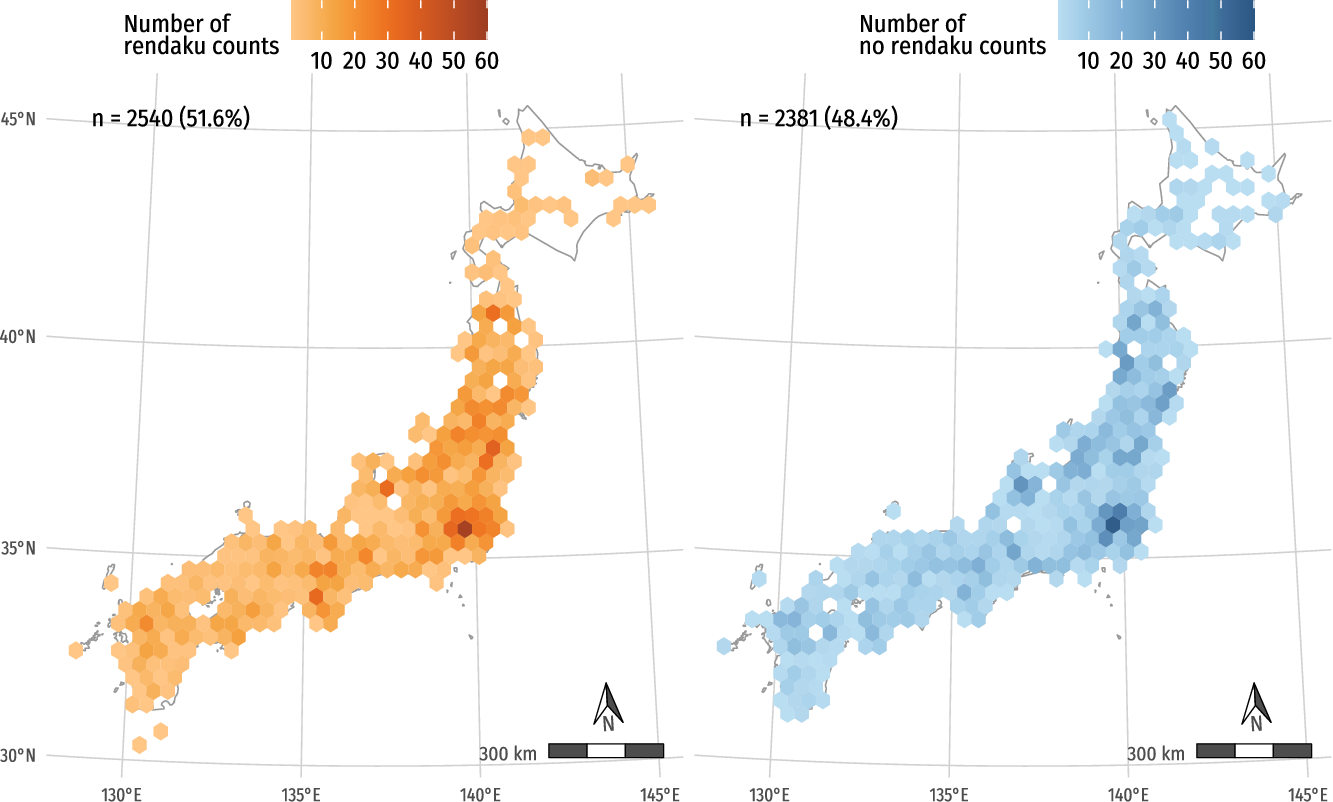
Map 2. Presence versus absence of rendaku in all place names.

Map 3. Presence versus absence of rendaku by lexeme.

2.2 Statistical analysis

In order to investigate whether the spatial distribution of rendaku is random or follows a pattern, we need to measure the spatial autocorrelation for the variable of interest, that is, the degree to which observations of presence versus absence of rendaku agree between neighboring place names. First, we defined a location’s neighbors as the set of all locations within a radius of 50 km of that location (Figure 1), which results in a circle with an area roughly equal to the mean area of Japanese prefectures without the Ryukyu Islands (7,982 km²).

Figure 1. Density distribution of the number per location of neighbors within a 50 km distance; vertical white lines indicate the quartiles (Q ₁ = 79, Q ₂ = 116, Q ₃ = 155, $$\bar x$$ = 128.8).

For exploratory purposes, a global join count (Moran, Reference Moran1948) was computed, with three different measures: J _BB, the number of neighboring locations that exhibit rendaku (“black-black”); J _WW, the number of neighboring locations that do not exhibit rendaku (“white-white”); and J _BW, the number of neighboring locations that exhibit opposite values (“black-white”).Footnote ⁶ The results (Table 3) indicate the existence of a statistically significant (z = 2.02, p = 0.02, one-sided test) positive spatial autocorrelation for J _BB, that is, place names exhibiting rendaku tend to co-occur more often than would be expected by chance alone.

Table 3. Global join count statistics

However, though the global join count indicates the existence of rendaku clusters, it does not specify where these clusters are located. In order to locate these clusters, the local indicator of spatial association for binary marked points proposed by Anselin and Li (Reference Anselin and Li2019) was calculated for each location with a place name exhibiting rendaku as the number of its neighbors that also exhibit rendaku.Footnote ⁷ Then, a conditional permutation test with 999 repetitions was performed in order to obtain for each location the pseudo p-value of getting, by chance, an indicator at least as high as observed. Since many tests were performed, the false discovery rate of multiple hypothesis testing was controlled by applying the procedure of Benjamini and Hochberg (Reference Benjamini and Hochberg1995) in accordance with Castro and Singer (Reference Castro and Singer2006). Locations with an adjusted p-value below the .05 α-level were considered to constitute cores of rendaku clusters, and the neighbors of those cores that exhibit rendaku were also considered to be part of the clusters, since, even though their indicator is not significant by itself, it contributes to make those of the cores significant.

Such cores and their neighbors exhibiting rendaku were then submitted to an unsupervised density-based cluster analysis with the DBSCAN algorithm (Ester et al., Reference Ester, Kriegel, Sander, Xu, Simoudis, Han and Fayyad1996) with parameters ϵ = 50 km and MinPts = 30.

All analyses were performed using the R Statistical Software (v4.2.1, R Core Team, 2022) and the spdep (v1.2.5, Bivand, Pebesma, & Gómez-Rubio, Reference Bivand, Pebesma and Gómez-Rubio2013) and dbscan (v1.1.10, Hahsler, Piekenbrock, & Doran, Reference Hahsler, Piekenbrock and Doran2019) packages. Geospatial data was processed using the R package sf (v1.0.8, Pebesma, Reference Pebesma2018).

3. Results

The statistical analysis of local spatial association indicates the existence of 167 cores of clusters, which represent 3.4% of all locations and 6.6% of locations exhibiting rendaku. These are surrounded by a total of 376 neighbors, which themselves represent 7.6% of all locations and 14.8% of locations exhibiting rendaku. Conversely, 78.6% of place names exhibiting rendaku do not belong to a cluster. Map 4 shows the location of the cores of clusters.

Map 4. Cores of rendaku clusters.

These cores and neighbors form two different geographical cluster areas, as revealed by both the visual inspection of the data (Map 5) and the application of the clustering algorithm. Table 4 and Table 5 summarize the number of cores and neighbors by cluster area and, respectively, prefecture and lexeme.

Map 5. Cores (full colors) of rendaku clusters and their neighbors (dimmed colors).

Map 6. Cores (full colors) of individual rendaku cluster areas and their neighbors (dimmed colors).

Table 4. Number of cores and neighbors by area and prefecture

Table 5. Number of cores and neighbors by area and lexeme

4. Discussion

We observed that place names exhibiting rendaku are not distributed completely at random across Japan but tend to co-occur in some areas, and we detected two different geographical rendaku cluster areas. This contrasts with the findings of Takemura et al. (Reference Takemura, Pellard, Kyung Hwang and Vance2019): that there is no clear geographical pattern. The major problem with that preliminary study is that it ignored the problems of spatial autocorrelation and calculated the mean rendaku rate by prefecture, though there is little justification for believing that dialectal zones and their differences in rendaku rate strictly follow the boundaries of modern administrative units. This probably had the unfortunate consequence of masking the existence of rendaku clusters distributed over several prefectures, as revealed in our more fine-grained study. It also suffers from a lack of homogeneity in the rendaku rate of the different lexemes studied.

Tamaoka and Ikeda (Reference Tamaoka and Ikeda2010) conclude that dialect has no influence on rendaku frequency. Their study is based on an experiment with 405 speakers from six different localities (Kagoshima, Ōita, Fukuoka, Yamaguchi, Hiroshima, and Shizuoka). However, their conclusion is expected from our perspective, since none of these prefectures belongs to a rendaku cluster area.

Similarly, Irwin and Vance (Reference Irwin and Vance2015) record the absence of presence of rendaku in 32 examples of 31 lexemes in the speech of 67 speakers of dialects from four different regions (Yamagata, Ehime, Miyazaki, and Hyōgo) but do not find a significant difference in average rendaku rate across locations. From our perspective, no such difference is indeed expected between Ehime, Miyazaki, and Hyōgo: Ehime and Miyazaki do not belong to a rendaku cluster area, and Hyōgo only contains a few neighbors. On the other hand, Yamagata contains several cores of rendaku clusters, and our results are thus at variance with theirs.

Asai (Reference Asai2014) found rendaku to be slightly more frequent in Northeastern Japanese dialect recordings (58%) than in Standard Japanese (50%).Footnote ⁸ His sample of Northeastern Japanese consists of dialects from Aomori, Akita, Iwate, Miyagi, Yamagata, and Fukushima, which substantially overlaps with our rendaku cluster area A. Such results are thus compatible with ours and are at variance with those of Irwin and Vance (Reference Irwin and Vance2015).

The existence of a large rendaku cluster area in Northeast Japan is interesting, since it is known that in dialects of that region, the voiceless versus voiced distinction is realized differently than in Standard Japanese; that is, in intervocalic position, voiceless stops are realized as voiced and voiced ones as prenasalized (Miyashita et al., Reference Miyashita, Irwin, Wilson, Vance, Vance and Irwin2016). It is, however, unlikely that this cluster area is the result of place names without rendaku but intervocalic voicing erroneously recorded as exhibiting rendaku. Though the consonant s does not undergo intervocalic voicing, half of the lexemes examined have an initial s-, and as much as 13.3% of the place names in cluster area A involve a lexeme with an initial s-.

5. Conclusions

This article shows the benefits of fine-grained analyses of spatial statistics for the study of linguistic variation and how a new measure of local spatial autocorrelation can be applied to linguistic categorical variables for detecting and localizing clusters. We were able to show that the frequency of rendaku varies across Japanese regions, and we detected the existence of two cluster areas of rendaku that could not be detected by simply looking at the data or by averaging frequency by prefecture and that had not been identified by previous studies.

Our study used place names to investigate the spatial variation of rendaku frequency. This raises the problem of the reliability of our data as a representative sample of dialects. Place names are often ancient and can predate the formation of the modern dialects, and the origin of their current pronunciation is unknown. Moreover, there is no assurance that the recorded place names readings that we used are always the same as the pronunciations in actual use locally.

Nevertheless, our statistical procedure detected a spatial pattern that cannot be reasonably attributed to chance only and that needs to be explained, in any case. Moreover, we think of place names as a proxy for a pandialectal study covering all Mainland Japan, which is unfeasible by the means of traditional dialectology. We recommend that the spatial cluster areas of rendaku that we detected be subjected to conventional dialectological surveys in order to try to replicate our results with experimental data. In other words, we suggest that further dialectal studies of rendaku start by looking at the areas of Fukushima-Yamagata and Wakayama.

Data availability statement

The data and code used for this study are openly available in an Open Science Framework repository at http://doi.org/10.17605/OSF.IO/MA8Q7.

Footnotes

1 One of the first applications of spatial statistics to linguistic data is Lee and Kretzschmar (Reference Lee and Kretzschmar1993). See Grieve (Reference Grieve, Boberg, Nerbonne and Watt2018) for an overview.

2 The consonant h alternates with b due to a sound change *p > h in the history of Japanese.

3 See Vance (Reference Vance and Kubozono2015) for an introduction to the topic, and Vance and Irwin (Reference Vance and Irwin2016) for a thorough review of the issues and the relevant literature.

4 https://geocode.csis.u-tokyo.ac.jp/.

5 Additional geospatial data for mapping was obtained from the GADM database (v.4.1, Global Administrative Areas, 2018).

6 Formally, with x _i and x _j the value of the variable x of presence (x = 1) vs. absence (x = 0) of rendaku at respectively locations i and j (i ≠ j), ${J_{BB}} = {1 \over 2}\sum {\sum {{w_{ij}}} } {x_i}{x_j}$ , ${J_{WW}} = {1 \over 2}\sum {\sum {{w_{ij}}} } \left( {1 - {x_i}} \right)\left( {1 - {x_j}} \right)$ , and ${J_{BW}} = {1 \over 2}\sum {\sum {{w_{ij}}} } {\left( {{x_i} - {x_j}} \right)^2}$ . The value of w _ij is specified by a symmetrical binary spatial weights matrix, where w _ij = 1 if locations i and j are neighbors and w _ij = 0 otherwise.

7 Formally, the indicator is defined in way similar to the global join count, as $B{B_i} = {x_i}\sum {{w_{ij}}} {x_j}$ . The indicator BB _i boils down to 0 if there is no rendaku (x _i = 0), and the contribution of other locations is zero when they are not a neighbor of i (w _ij = 0) or when they do not themselves exhibit rendaku (x _j = 0). Each neighbor exhibiting rendaku has a contribution of w _i,j x _j = 1.

8 Asai (Reference Asai2014) did not perform a significance test, and he does not present all the relevant figures.

References

Anselin, Luc. 1995. Local indicators of spatial association—LISA. Geographical Analysis 27(2). 93–115. https://doi.org/10.1111/j.1538-4632.1995.tb00338.x.CrossRef Google Scholar

Anselin, Luc & Li, Xun. 2019. Operational local join count statistics for cluster detection. Journal of Geographical Systems 21(2). 189–210. https://doi.org/10.1007/s10109-019-00299-x.CrossRef Google Scholar PubMed

Asai, Atsushi. 2014. Rendaku seiki no keikō to teichakuka. NINJAL Research Papers 7. 27–44. https://doi.org/10.15084/00000523.Google Scholar

Benjamini, Yoav & Hochberg, Yosef. 1995. Controlling the false discovery rate: A practical and powerful approach to multiple testing. Journal of the Royal Statistical Society: Series B (Methodological) 57(1). 289–300. https://doi.org/10.1111/j.2517-6161.1995.tb02031.x.Google Scholar

Bivand, Roger S., Pebesma, Edzer & Gómez-Rubio, Virgilio. 2013. Applied spatial data analysis with R. 2nd edn. New York: Springer. https://doi.org/10.1007/978-1-4614-7618-4.CrossRef Google Scholar

Castro, Marcia Caldas de & Singer, Burton H.. 2006. Controlling the false discovery rate: A new application to account for multiple and dependent tests in local statistics of spatial association. Geographical Analysis 38(2). 180–208. https://doi.org/10.1111/j.0016-7363.2006.00682.x.CrossRef Google Scholar

Ester, Martin, Kriegel, Hans-Peter, Sander, Jörg, & Xu, Xiaowei. 1996. A density-based algorithm for discovering clusters in large spatial databases with noise. In Simoudis, Evangelos, Han, Jiawei & Fayyad, Usama M. (eds.), Proceedings of the Second International Conference on Knowledge Discovery and Data Mining (KDD-96), 226–231. Menlo Park: Press. https://www.aaai.org/Papers/KDD/1996/KDD96-037.pdf.Google Scholar

Global Administrative Areas. 2018. GADM database of global administrative areas. http://www.gadm.org.Google Scholar

Goebl, Hans. 2018. Dialectometry. In Boberg, Charles, Nerbonne, John, & Watt, Dominic (eds.), The handbook of dialectology, 123–42. Hoboken: Wiley. https://doi.org/10.1002/9781118827628.ch7.Google Scholar

Grieve, Jack. 2011. A regional analysis of contraction rate in written Standard American English. International Journal of Corpus Linguistics 16(4). 514–46. https://doi.org/10.1075/ijcl.16.4.04gri.CrossRef Google Scholar

Grieve, Jack. 2013. A statistical comparison of regional phonetic and lexical variation in American English. Literary and Linguistic Computing 28(1). 82–107. https://doi.org/10.1093/llc/fqs051.CrossRef Google Scholar

Grieve, Jack. 2018. Spatial statistics for dialectology. In Boberg, Charles, Nerbonne, John & Watt, Dominic (eds.), The handbook of dialectology, 415–33. Hoboken: Wiley. https://doi.org/10.1002/9781118827628.ch24.Google Scholar

Grieve, Jack, Speelman, Dirk, & Geeraerts, Dirk. 2011. A statistical method for the identification and aggregation of regional linguistic variation. Language Variation and Change 23(2). 193–221. https://doi.org/10.1017/S095439451100007X.CrossRef Google Scholar

Grieve, Jack, Speelman, Dirk, & Geeraerts, Dirk. 2013. A multivariate spatial analysis of vowel formants in American English. Journal of Linguistic Geography 1(1). 31–51. https://doi.org/10.1017/jlg.2013.3.CrossRef Google Scholar

Hahsler, Michael, Piekenbrock, Matthew, & Doran, Derek. 2019. dbscan: Fast density-based clustering with R. Journal of Statistical Software 91(1). 1–30. https://doi.org/10.18637/jss.v091.i01.CrossRef Google Scholar

Irwin, Mark & Vance, Timothy J.. 2015. Rendaku across Japanese dialects. Phonological Studies 18. 19–26. https://www.researchgate.net/publication/332141508_Rendaku_Across_Japanese_Dialects.Google Scholar

Post, Japan. 2014. Yūbin bangō dēta. https://www.post.japanpost.jp/zipcode/download.html.Google Scholar

Lee, Jay & Kretzschmar, William A.. 1993. Spatial analysis of linguistic data with GIS functions. International Journal of Geographical Information Systems 7(6). 541–60. https://doi.org/10.1080/02693799308901981.CrossRef Google Scholar

Miyashita, Mizuki, Irwin, Mark, Wilson, Ian, & Vance, Timothy J.. 2016. Rendaku in Tōhoku Japanese: The Kahoku-chō survey. In Vance, Timothy J. & Irwin, Mark (eds.), Sequential voicing in Japanese: Papers from the NINJAL Rendaku Project, 173–94. Amsterdam: John Benjamins. https://doi.org/10.1075/slcs.176.10miy.Google Scholar

Moran, Patrick A. P. 1948. The interpretation of statistical maps. Journal of the Royal Statistical Society: Series B (Methodological) 10(2). 243–51. https://www.jstor.org/stable/2983777.Google Scholar

Ord, J. K. & Getis, Arthur. 1995. Local spatial autocorrelation statistics: Distributional issues and an application. Geographical Analysis 27(4). 286–306. https://doi.org/10.1111/j.1538-4632.1995.tb00912.x.CrossRef Google Scholar

Pebesma, Edzer. 2018. Simple features for R: Standardized support for spatial vector data. The R Journal 10(1). 439. https://doi.org/10.32614/rj-2018-009.CrossRef Google Scholar

R Core Team. 2022. R: A language and environment for statistical computing. Vienna: R Foundation for Statistical Computing. https://www.R-project.org.Google Scholar

Shimoji, Michinori & Pellard, Thomas (eds.). 2010. An introduction to Ryukyuan languages. Tokyo: Research Institute for Languages and Cultures of Asia and Africa.Google Scholar

Takemura, Akiko, Pellard, Thomas, Kyung Hwang, Hyun & Vance, Timothy J.. 2019. Rendaku in place names across Japanese dialects. Reports of the Keio Institute of Cultural and Linguistic Studies 50. 79–89. http://koara.lib.keio.ac.jp/xoonips/modules/xoonips/detail.php?koara_id=AN00069467-00000050-0079.Google Scholar

Tamaoka, Katsuo & Ikeda, Fumiko. 2010. Whiskey or bhiskey? Influence of first element and dialect region on sequential voicing of shoochuu . Gengo Kenkyū 37. 65–79. https://doi.org/10.11435/gengo.137.0_65.Google Scholar

Vance, Timothy J. 2015. Rendaku. In Kubozono, Haruo (ed.), Handbook of Japanese phonetics and phonology, 397–441. Berlin: De Gruyter Mouton. https://doi.org/10.1515/9781614511984.397.CrossRef Google Scholar

Vance, Timothy J. & Irwin, Mark (eds.). 2016. Sequential voicing in Japanese: Papers from the NINJAL Rendaku Project. Amsterdam: John Benjamins. https://doi.org/10.1075/slcs.176.CrossRef Google Scholar

Wieling, Martijn & Nerbonne, John. 2015. Advances in dialectometry. Annual Review of Linguistics 1(1). 243–264. https://doi.org/10.1146/annurev-linguist-030514-124930.CrossRef Google Scholar

Table 1. Rendaku rate by lexeme (original data of Takemura et al., 2019)

Map 1. Map of the 4,921 locations investigated.

Table 2. Rendaku rate by lexeme (filtered and geocoded data)

Map 2. Presence versus absence of rendaku in all place names.

Map 3. Presence versus absence of rendaku by lexeme.

Figure 1. Density distribution of the number per location of neighbors within a 50 km distance; vertical white lines indicate the quartiles (Q1 = 79, Q2 = 116, Q3 = 155, $$\bar x$$ = 128.8).