

Even under the conditions of pure competition and static demand and supply, there is thus no “automatic self-regulating mechanism”, which can provide full utilization of resources. Unemployment, excess capacity, and the wasteful use of resources may occur even when all the competitive assumptions are fulfilled.
—Ezekiel Reference Ezekiel1938, p. 279I. INTRODUCTION
From the classical metaphor of the invisible hand to the neoclassical Pareto optimality of perfect competition, theoretical and empirical claims about market stability lie at the core of orthodox economics. Confronted by cycles, sometimes unstable, in prices and production, belief in the self-regulating market mechanism has fostered a gradual evolution in models of market equilibrium. Essential features of this evolution are the shift from deterministic to stochastic modeling and recognition of the recursive role that producer price expectations have in determining future supply. Cobweb theory has played an essential role incorporating both features as explanations for endogeneity of price and production cycles in commodity markets. Empirical testing of cobweb models explored the possibility that “short run” supply and demand elasticities could produce temporary market instability. Subsequent evolution in the role of price expectations in cobweb theory—from naive to adaptive to rational expectations—generated fundamental change in theoretical conditions that validate claims of market stability.
Given the number of substantive contributions by important economists, lack of attention to cobweb theory in the history of economic thought on stability of market equilibrium is perplexing. A partial listing of contributors to this topic includes Jan Tinbergen (Reference Tinbergen1930); Henry Schultz (Reference Schultz1930a, Reference Schultz1930b); Nicholas Kaldor (Reference Kaldor1934); Wassily Leontief (Reference Leontief1934); Ronald Coase (Reference Coase and Fowler1935); Paul Samuelson (Reference Samuelson and Ellis1944, Reference Samuelson1976); Marc Nerlove (Reference Nerlove1958a, Reference Nerlove1958b); and John Muth (Reference Muth1961). Cobweb theory appears in models of endogenous cycles in prices and production and empirical studies of agricultural phenomena such as the hog price cycle. In conjunction with motivating development from naive expectations to adaptive expectations to rational expectations, cobweb theory also played a role in the evolution of recursive models for endogenous cycles in prices and production using linear difference equations to non-linear models of market equilibrium that can admit complex cyclic or chaotic properties, e.g., Cars Hommes (Reference Hommes1992); and Jason Galas and Helena Nusse (Reference Gallas and Nusse1996). As such, cobweb theory directs attention to empirical and theoretical properties associated with stability of markets. The model continues to attract contributions, e.g., Christophe Gouel (Reference Gouel2012); Simon Glöser-Chahoud et al. (Reference Glöser-Chahoud, Johannes Hartwig and Faulstich2016); Muhammad Chaudhry and Mario Miranda (Reference Chaudhry and Miranda2018).
After a review of the prehistory traceable to nineteenth- and early twentieth-century contributions that identified recurring cycles in commodity prices and production, this paper details the “first wave” of linear cobweb models during the 1930s, which introduced the theoretical possibility of endogenous market instability and clarified the distinction between static and dynamic equilibrium. Subsequent empirical studies by agricultural economists explored difficulties of estimating demand and supply elasticities associated with the generation of cycles arising in commodity markets predicted by cobweb theory. In turn, theoretical attacks on the possibility of market instability identified by cobweb theory suggested “improvements” that included introduction of non-linear supply and demand curves; “velocity of adjustment”; competitive storage and risk; vertically linked markets; and the like. Over time, the lynchpin of improvements involved the evolution of price expectations, from the initial naive model of first wave cobweb theory to the second wave incorporating adaptive expectations and, eventually, the random dynamics of rational expectations.
II. PREHISTORY TO THE FIRST WAVE
According to Mordecai Ezekiel (Reference Ezekiel1938, p. 255), the origin of cobweb theory occurs in 1930 when “three economists, in Italy [Umberto Ricci], Holland [Tinbergen], and the United States [Schultz], apparently independently, worked out the theoretical explanation which has since come to be known as the ‘cob-web theorem.’”Footnote 1 The etymology of “cobweb theorem” can be traced to Kaldor (Reference Kaldor1934, p. 134), though Leontief (Reference Leontief1934, in German) also refers to “Spinnwebenbild.” Being concerned with explaining “regularly recurring cycles in the production and prices of particular commodities” (Kaldor Reference Kaldor1934, p. 134), this first wave linear cobweb theory was preceded by a prehistory of contributions that identified cobweb-type behavior associated with prices for grains and other commodities. The earliest such contribution appears in Traité des grains (Reference Boisguilbert1704, short title) by the Enlightenment “philosopher” Pierre de Boisguilbert (1646–1714) with an empirical observation about cobweb-like behavior of French grain prices (Spengler Reference Spengler1984). However, Boisguilbert did not develop an analytical explanation for such empirical observations and this contribution either had little impact or was “swallowed up” in the “anonymity … relating to the impact of late seventeenth and early eighteenth century writers” (Spengler Reference Spengler1984, p. 89).
Other prehistory contributions from the first half of the nineteenth century with endogenous dynamics that focused on pricing and production of agricultural commodities include the debate surrounding the Corn Laws where Robert Torrens, Thomas Malthus, and John R. McCulloch proposed “cobweb-like” explanations that “stressed … corn laws magnified fluctuations in the price of corn by preventing the full adjustment of supply and demand following variations in crops” (Besomi Reference Besomi2008, p. 633). In 1839, James Wilson proposed an earlier version of cobweb-like theory that explained “fluctuations in grain supply and prices in terms of output in earlier years” (Boot Reference Boot1983, p. 567). Endogenous price dynamics also appear in explanations of market instability associated with economic crises, e.g., Robert Link (Reference Link1959) and Daniele Besomi (Reference Besomi2008). Explanations of crises based on endogenous dynamics differed from reliance on exogenous factors, such as crop failures, wars, trade embargoes, and the like, which resulted in a return to stability of “normal conditions” once the exogenous influence had dissipated. Though William Huskisson, Thomas Tooke, and others did propose explanations for economic crises that had endogenous features, only a few further proposed that such endogenous dynamics were cyclical. Besomi (Reference Besomi2008) identifies less well-known figures—John Wade, Hyde Clark, and James Wilson—who were early proponents of endogenous cycles.Footnote 2
By the end of the nineteenth century, acceptance of endogenous dynamics generating economic cycles with fixed periodicity was common, Stanley Jevons being but one such proponent. With the rise of neoclassical economics, the marginalist revolution, and increasing dependence on formal mathematics, such acceptance also coincided with the origins of modern econometrics (Turner and Wood Reference Turner and Wood2020, p. 509). This evolution in economic thought followed two general lines of development. In contrast to the mathematical “pure economics” of the Walrasian general equilibrium model, seminal contributions of Vilfredo Pareto, Francis Y. Edgeworth, and Jevons were characterized by additional rigor and precision provided by incorporating empirical and analytic methodologies of physics and other natural sciences. The latter line generated several decades of concern about distinguishing between statics and dynamics. Alfred Marshall (Reference Marshall1898, p. 37) provides an initial perspective: “The terms Economic Statics and Dynamics (or Kinetics) are imported from physics; and some discussions about them have seemed to imply that statics and dynamics are distinct branches of physics. But of course they are not.” It is on this landscape of economic thought that Henry Ludwell Moore made numerous contributions that, eventually, led to the emergence of first wave cobweb theory.
An odd feature of the noted summary by Ezekiel (Reference Ezekiel1938) covering the emergence and early evolution of cobweb theory is the treatment of Moore, mentioned only in relation to Ricci (Reference Ricci1930), which is a response to comments about Ricci made in Moore (Reference Moore1929, pp. 28–32). Cobweb theory represents the next step after Moore in explaining “the moving equilibrium of demand and supply” that Moore (Reference Moore1925, Reference Moore1929) was seminal in formulating. Moore was supervisor for the 1925 PhD thesis of Henry Schultz—“Estimation of Demand Curves”—which provided a foundation for later work on estimation of commodity demand functions. That Moore was a strong influence on later theoretical and empirical work by Schultz is evident in praise Schultz gives Moore in various studies. Tinbergen (Reference Tinbergen1930) recognizes Moore (Reference Moore1925) and Schultz (Reference Schultz1928) as motivations for introduction of cobweb dynamics to explain the relationship between the tendency toward static equilibrium of supply and demand and persistence of observed cycles in prices. Use of an econometric model with a supply function using a lagged price combined with a demand function dependent on current price as an explanation for cyclical behavior arguably originates with Moore (Reference Moore1925) (Schultz Reference Schultz1928; Morgan Reference Morgan1990, p. 170).
Moore (Reference Moore1929) is largely concerned with developing theoretical and statistical properties of the “Law of Supply and Demand.” Observing that, for Marshall, “treatment of particular equilibria is hypothetical, static, and limited to functions of one variable,” Moore (Reference Moore1929, p. 94) adopts the following empirical approach to the theoretical dynamic moving equilibrium solution proposed by Léon Walras in the Elements, “which re-establishes itself automatically as soon as it is disturbed”: “The problem of a moving equilibrium of demand and supply when both demand and supply are functions of one variable alone may, therefore, be treated empirically by the methods with which we have become acquainted [correlation and linear regression]” (Reference Moore1929, p. 94).
In the process of empirically determining the moving equilibrium of supply and demand for potatoes, Moore (Reference Moore1925, p. 370; Reference Moore1929, p. 97) makes a seminal statistical contribution—what Schultz (Reference Schultz1928, ch. v) refers to as “the lag method”—that becomes an essential feature of first wave cobweb theory. Schultz (Reference Schultz1928, p. 126) observes: “Professor Moore does not give a detailed explanation of his method, but an examination of the way in which he uses the same data to obtain both the demand curve and the supply curve leaves no doubt as to the rationale of it.” Moore provides the following initial presentation for statistical estimation of the “Law of Supply and Demand” using the lag method depicted with a so-called Marshallian partial equilibrium supply-demand diagram:

Source: Moore (Reference Moore1925, p. 370).
In the diagram x is equilibrium quantity, pd is current price, and ps is price lagged one period with all variables being de-trended.Footnote 3
It is unfortunate that presentation of the theoretical model proposed by Moore in his “Figure 2” was adjusted by Mary Morgan (Reference Morgan1990, p. 170) and George Stigler (Reference Stigler1962, p. 16). Using notation that seemingly suppresses recognition of the “trend ratios” used by Moore, Morgan reformulates the moving equilibrium of demand and supply in a more modern format as:
 $$ Demand\ Equation\hskip0.96em {P}_t={a}_0+{a}_1\;{Q}_t^D $$
 $$ {\displaystyle \begin{array}{c} Supply\ Equation\hskip1.32em {Q}_t^S={b}_0+{b}_1\;{P}_{t-1}\\ {} where\hskip0.6em {Q}_t^D={Q}_t^S\end{array}} $$
The notation Q replaces x, time dating is introduced, and having the supply equation with Q on the left-hand side is more consistent with subsequent formulations of cobweb theory. In contrast, Stigler follows the formulation given in Tinbergen (Reference Tinbergen1930) and inverts results given by Moore to:
 $$ {\displaystyle \begin{array}{c}{x}_{dt}=1.702-.702\;{p}_t\\ {}{x}_{st}=.181+.801\;{p}_{t-1}\end{array}} $$
Though these alternative formulations to that used by Moore are more consistent with those employed in subsequent cobweb theory presentations, historical context is obscured. As indicated in both Schultz (Reference Schultz1928, pp. 176–178) and Moore (Reference Moore1925, p. 368), the actual estimations involved prices being regressed on quantities. Whether or not Moore was proposing a model of market stability with naive price expectations where both price and quantity were endogenously determined is left unresolved. The econometric procedure of estimating a reduced form and solving for the structural coefficients is not employed.
Oddly, empirical parameter estimates provided by Moore in his “Figure 2” seemingly indicate market instability. Though Moore does not recognize this implication, the first wave contribution by Ricci shows that the supply lag estimated by Moore, if written as a dynamic problem, produces increasing oscillations around the equilibrium if unperturbed. While complementary to Moore, Ricci (Reference Ricci1930, p. 656) observes: “So the equilibrium, once broken, is lost forever. The American economy is, at least as far as the potatoes are concerned, at the mercy of the tragic fate of a growing disequilibrium!” Ricci proceeds to show that slightly changing parameters of the supply curve is enough to obtain either a sustained cycle for a restricted parameter range or a damped cycle for a wider range of parameters. As such, Ricci clearly demonstrated fragility of economic stability associated with market fluctuations. Despite the careful development of assumptions in Moore (Reference Moore1929), Ricci (Reference Ricci1930, p. 657) was able to show “he failed to meet the much more vital requirement that his equilibrium should be stable.”Footnote 4
III. FIRST WAVE COBWEB THEORY
The history of cobweb theory has distinct roots in the diverse emerging fields of econometrics and agricultural economics. In econometrics, connections between early contributors to cobweb theory and the Econometric Society are numerous. Henry Schultz was one of sixteen founding members of the Society in 1930 and, together with Tinbergen and Ricci, was one of the first 1933 list of Fellows. Mordecai Ezekiel was named Fellow in 1935. Other important contributors to cobweb theory were also later named Fellows: Leontief in 1939, Samuelson in 1944, Kaldor in 1945, Nerlove in 1960, and Muth in 1968. Also included in the list of Fellows are several who were important to the prehistory and contributions to empirical work: Henry Moore in 1933, Elmer Working in 1945, and Holbrook Working in 1947. As such, the emergence of cobweb theory represents a substantive step in the evolution of “economic science” beyond the theoretical frameworks of Antoine-Augustin Cournot, Edgeworth, Walras, and Pareto that motivated the “statistical economics” and “synthetic economics” Moore used to explore empirical estimation of supply and demand functions with linear regression and correlation techniques.
With hindsight, it is apparent that numerous confusions and limitations are associated with the “moving equilibrium of supply and demand” proposed by Moore. The cobweb theory of Ricci and Tinbergen originates as a demonstration that Moore was incorrect in concluding market stability equilibrium will necessarily be restored following perturbation to supply or demand.Footnote 5 Yet, despite some shortcomings, the contributions of Moore were significant enough for Tinbergen (Reference Tinbergen1951, p. 9) to observe: “[E]conometrics had its precursors even before it was christened. Econometricians like to think of Cournot the same way as economists think of Adam Smith, whereas the great modern precursor or, rather, pioneer has been Moore.” Among others, this view was shared by Stigler (Reference Stigler1962, p. 1):
If one seeks distinctive traits of modern economics, traits which are not shared to any important degree with the Marshallian or earlier periods, [they] will find only one: the development of statistical estimation of economic relationships…. Henry Moore was its founder, in the sense in which most large movements have a founder. He had gifted predecessors and contemporaries; but no one else was so persistent, so ambitious, or so influential as he in the development of this new approach.
Appearing the year following the retirement of Moore due to “illness,” the same year as the founding of the Econometric Society, cobweb theory coincides with the first steps along the path to modern econometrics and economic dynamics.
The initial first wave cobweb theory by Schultz, Tinbergen, and Ricci appearing in 1930 had some distinctive features. As with the important contribution by Leontief (Reference Leontief1934), these publications were in German sources, leaving presentation of early cobweb models in English publications to contributions such as Kaldor (Reference Kaldor1934), Ronald Coase and Ronald Fowler (Reference Coase and Fowler1935), Ludwig Lachmann (Reference Lachmann1936), and Ezekiel (Reference Ezekiel1938).Footnote 6 The original three first wave contributions are described by Ezekiel (Reference Ezekiel1938, p. 256):
Schultz’s demonstration was the simplest, presenting merely one example of the convergent type, but also plotting the resulting time-series of prices and quantities. Tinbergen’s analysis was more complete, presenting both the convergent and divergent types…. Ricci’s analysis … presented diagrams of all three basic types, convergent, divergent, and continuous.
In turn, the linguistic barrier disguised motivations of the contributors. Tinbergen and Schultz were primarily concerned with “econometric” issues surrounding the relationship between theoretical dynamic stability of market equilibrium and estimation of demand and supply functions. Though Moore (Reference Moore1925) had proposed a solution to the problem of reconciling empirical cycles in dynamics of certain commodity prices with theoretical notions of static market equilibrium advanced by Cournot, Walras, and Marshall—a solution involving a demand function based on current price and a supply function depending on price in the previous period—the Ricci and Tinbergen contributions to first wave cobweb theory aimed to correct inadequate interpretation of the dynamic model proposed by Moore.
Despite a common concern with cobweb theory, each of the seminal contributions reflects a different perspective. For instance, Tinbergen (Reference Tinbergen1930) was different from Ricci and Schultz in focusing on the econometric identification problem associated with determining parameters of the supply and demand functions from a time series. Moore handled this problem by introducing what Schultz (Reference Schultz1928) referred to as “the lag method” of shifting the column of prices and quantities down one unit to obtain two different equations for estimating supply and demand. Use of this mechanical approach explains why Moore viewed “the moving equilibrium of demand and supply” as inherently convergent, overlooking the problem of potential dynamic instability associated with cobweb theory. Tinbergen recognized the lag method was an ingenious solution to the identification problem compared with other approaches such as that in Leontief (Reference Leontief1929). Tinbergen presented cobweb theory to demonstrate that the lag model dynamics were problematic as market stability required restrictions on parameters of the supply and demand functions: “the mechanism given here either leads to ever increasing fluctuations or to the rapid establishment of an equilibrium position” (Tinbergen Reference Tinbergen1930, p. 670).
Though Schultz (Reference Schultz1930a, Reference Schultz1930b) did also focus on econometric issues that concerned Tinbergen, the narrative was decidedly different from Tinbergen’s. The preamble by the editors of Zeitschrift für Nationalökonomie to the contribution by Ricci (Reference Ricci1930) captures the context: “This study is the first in a series of four papers in which the author examines the latest trends and findings in American economics.” Representing the “American” approach, Schultz aimed to promote advances in “statistical economics” introduced by Moore and extended in Schultz (Reference Schultz1928). There is a detailed discussion of empirical failings of Leontief (Reference Leontief1929), leading Schultz (Reference Schultz1930b, pp. 99–118) to conclude: “both of Leontief’s coefficients of elasticity are numerical accidents having no economic meaning.” The statistical economics of the American approach to “demand curves” is contrasted with the “statical” neoclassical, ceteris paribus approach of Marshall, “a special case of the general demand function of the mathematical school” associated with Walras and Pareto. Aiming to demonstrate the statistical approach to estimating the demand curve with a supply curve dependent on lagged price, it is not surprising that the only cobweb diagram (Schultz Reference Schultz1930b, p. 34, fig. IV) illustrating adjustment to disequilibrium is for the convergent case.
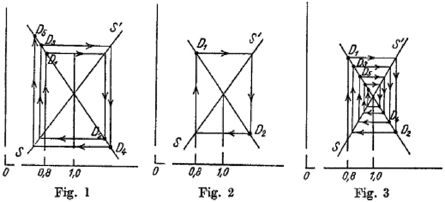
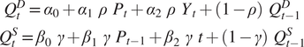
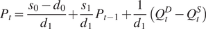
It is well known that the appellation “cobweb” is due to the graphical appearance of the price process following a perturbation to the demand or supply curve (see figures 1 and 2). These diagrams from the first wave contributions are the basis for presentations in Kaldor (Reference Kaldor1934), Ezekiel (Reference Ezekiel1938), Norman Buchanan (Reference Buchanan1939), and other sources. Close examination of the graphical structure of the cobweb diagrams situates first wave cobweb theory within “a wide spectrum of research and concepts that coalesced only in the 1930s, when the topics of ‘stability’ on the one hand, and ‘expectations’ on the other, polarized economic dynamics studies” (Tusset Reference Tusset2009, p. 267). Numerous insights and debates concerning the broader interpretation of statics, dynamics, and stationary state can be roughly divided into the “objective,” largely mathematical approaches based on analogies with mechanics, and the “subjective,” incorporating expectations and other psychological factors. The objective approach culminated in the correspondence principle of Paul Samuelson—e.g., Samuelson (Reference Samuelson1947)—and the calculus of variations approach initiated by Griffith Evans and Charles Roos and further developed by the Paretian school (Pomini Reference Pomini2018). While first wave cobweb theory largely advanced “objective” considerations, development of the subjective dimension characterizes the second wave.
Algebraic formulation of first wave cobweb graphs and conditions associated with market instability, adapted from Tinbergen, are illustrated in various sources, e.g., Nerlove (Reference Nerlove1958b, pp. 228–229), and Charles Ferguson (Reference Ferguson1960, p. 300):
 $$ {Q}_t^D={d}_0+{d}_1\;{P}_t\hskip1.8em {Q}_t^S={s}_0+{s}_1\;{P}_{t-1}\hskip1.44em {Q}_t^S={Q}_t^D $$
This leads to the linear first order difference equation and solution for equilibrium price PE and quantity QE when Pt = Pt-1 = PE:
 $$ {P}_t=\frac{s_0-{d}_0}{d_1}+\frac{s_1}{d_1}\;{P}_{t-1}\hskip1.68em {P}_E=\frac{s_0-{d}_0}{d_1-{s}_1}\hskip1.8em {Q}_E=\frac{s_1\;{d}_0-{d}_1\;{s}_0}{d_1-{s}_1} $$
The linear cobweb dynamics follow from starting in equilibrium and imposing a discontinuous perturbation such that PE ≠ P0 (due to an exogenous shift in supply or demand at t = 0) and observing that the path of prices starting from P0 depends on the relative slopes of the supply and demand curves: explosive oscillation for | s1 | > | d1 |; alternating oscillation for | s1 | = | d1 |; and converging oscillation for | s1 | < | d1 |.Footnote 7 Given the close relationship between elasticity and slope, these results can be expressed in terms of supply and demand elasticities for “curves of constant elasticity, reduced to linearity by using a logarithmic scale” (Newman Reference Newman1951, p. 336).Footnote 8 More precisely, “explosive oscillation” is associated with an absolute value for price elasticity of supply greater than the absolute value for price elasticity of demand. Potential sensitivity of the dynamics to specification of P0, a fundamental feature of chaotic processes, is not explicitly incorporated.
A now largely forgotten feature of first wave cobweb theory introduced by Schultz, Ricci, and Tinbergen is the relevance of historical context. Evolving on a landscape of economic crisis, first wave cobweb theory represented a plausible theoretical illustration of inherent instability in commodity prices and production at that time. As Ezekiel (Reference Ezekiel1938, pp. 278–279) observes: “classical economic theory rests upon the assumption that price and production, if disturbed from their equilibrium, tend to gravitate back toward that normal. Cobweb theory demonstrates that, even under static conditions, this result will not necessarily follow,” thus permitting a “non-classical” explanation for observed persistence in underemployment of the 1930s (Reference Ezekiel1938, pp. 278–279): “Even under the conditions of pure competition and static demand and supply, there is thus no ‘automatic self-regulating mechanism,’ which can provide full utilization of resources. Unemployment, excess capacity, and the wasteful use of resources may occur even when all the competitive assumptions are fulfilled.”
In this sense, first wave cobweb theory represented a substantive evolution from earlier “inherent stability” views of Moore (Reference Moore1929, p. 152): “Availing himself of a hint given by Cournot, Walras has shown how perturbations of a general equilibrium are diffused throughout the whole economic system, setting up oscillations which, with the flow of time, progressively diminish in amplitude until they are extinguished and equilibrium is restored.”
The implication of endogenous market instability arising from first wave cobweb theory generated various contributions seeking theoretical explanations to counter the possibility of such instability. Kaldor (Reference Kaldor1934) attacked cobweb theory for failing to account for distinction between short-run and long-run elasticities and the associated “velocity of adjustment.” Lachmann (Reference Lachmann1936) identified failure to incorporate inventory adjustment. Buchanan (Reference Buchanan1939) demonstrated that those cases where cobweb theory produces dynamic instability are unsustainable as “losses will inevitably exceed profits.” Such theoretical results were informed by a host of empirical studies by agricultural economists on cycles in commodity markets, in general, and the hog cycle, especially. The relevance of supply and demand elasticities to cobweb theory contributed to further empirical studies incorporating insights on estimation of demand functions by Herman Wold and others. Against this backdrop, the disturbing theoretical implication of cobweb theory that perfect competition could lead to dynamic instability was gradually replaced by concern in the second wave with expectations formation as a theoretical foundation for rationalizing market stability. The naive expectations of the first wave evolved into cobweb models with extrapolative (Goodwin Reference Goodwin1947), adaptive (Nerlove Reference Nerlove1958b), and rational (Muth Reference Muth1961) expectations of the second wave.
IV. COBWEBS IN AGRICULTURAL ECONOMICS
In addition to illustrating potential theoretical instability of the moving equilibrium of demand and supply proposed by Moore, first wave cobweb theory also stimulated seminal efforts in applied econometrics spearheaded by agricultural economists. Ezekiel (Reference Ezekiel1938, p. 272) identifies three theoretical conditions used to classify empirical failings of first wave cobweb theory, “even for commodities which approximately fulfill the assumptions”:
(1) … Production is completely determined by the producers’ response to price, under conditions of pure competition (where the producer bases plans for future production on the assumption present prices will continue, and that his own production plans will not affect the market); (2) … The time needed for production requires at least one full period before production can be changed, once the plans are made; and (3) the price is set by the supply available.
Similar to Schultz (Reference Schultz1928, ch. v; Reference Schultz1932), Ezekiel observed that, even if the production decision—such as acres planted—is made with a lag, it is possible to reduce production by, say, plowing under planted acres or not harvesting the crop. In addition, for many commodities the cost of inputs—such as the price of feed for livestock production—as well as commodity price impact the production decision.Footnote 9 Perhaps the most important variable impacting production for field crops is not price—which influences the acres planted—but weather—which impacts yield per acre. For products with long life, production in any period only adds to total supply, which is the variable that drives price. It is not supply alone that determines price. Demand can change depending on a range of variables such as the price of competing products, propensity to consume from income, transportation costs, and foreign supply.
In contrast to “objective” concerns of the seminal 1930 contributions, Ezekiel (Reference Ezekiel1938) is part of a stream of efforts focusing on relevance of first wave cobweb theory to “real world” situations in agricultural markets. Perhaps most well known is the so-called pork cycle, also referred to as the pig cycle or hog cycle, an empirical phenomenon that still attracts attention, e.g., Matthew Holt and Lee Craig (Reference Holt and Craig2006); and Phillip Parker and J. Scott Shonkwiler (Reference Parker and Shonkwiler2014). In an early study of cobweb theory in the UK market for pigs, Coase and Fowler (Reference Coase and Fowler1935, p. 142) reflect the distinction between theory and practical implications of cobweb theory for market stability:
The existence of a pig-cycle, in the sense of a self-perpetuating cycle of pig prices … excited some attention among theoretical economists as an example of the influence of the lack of foresight in causing disequilibrium. In economic theory, this argument is generally known as the ”cobweb theorem." If producers assume that present prices and costs will continue unchanged, and if there is a change in demand or supply conditions, then providing that the elasticities of demand and supply are of a certain order of magnitude, it can be shown that continuous fluctuations in prices and output will occur and that there will be no tendency for an equilibrium to be established.
Providing a detailed exploration of the market for pigs, Coase and Fowler demonstrate various practical reasons undermining naive price expectations of first wave cobweb theory as the basis for cyclical market behavior. The practical distinction between pig breeders and feeders is among the reasons why the expectation that “current prices and costs will continue” is “incorrect.” It is demonstrated that breeders tended to act immediately to changes in profitability, not with a lag. Instability in profits due to variation in costs was “probably unimportant,” with variations in demand and response of foreign producers “probably extremely important.” Instead of focusing on prices, profitability is “the really significant feature.”
As the survey by Robert Myers, Richard Sexton, and William Tomek (Reference Myers, Sexton and Tomek2010) details, empirical applications of cobweb theory by agricultural economists initially built on earlier studies of supply and demand. In addition to important contributions by Moore, Schultz, Holbrook Working (Reference Working1922), George Haas and Ezekiel (Reference Haas and Ezekiel1926), and Elmer Working (Reference Working1927), empirical work by Louis Bean (Reference Bean1929) indicated that “the dominant factor explaining changes in acreage and hog numbers was the price received by farmers in the preceding season. The price received two years preceding was also often important” (Myers, Sexton, and Tomek Reference Myers, Sexton and Tomek2010, p. 384). Recognizing that the “cobweb theorem … should be used … only for those commodities whose conditions of pricing and production satisfy the special assumptions on which it is based,” Ezekiel (Reference Ezekiel1938, p. 278; see discussion pp. 274–277) provided empirical evidence for potatoes similar to Bean’s. However, consistent with an explanation of market stability provided by Kaldor (Reference Kaldor1934), subsequent accumulating evidence that commodity price and production are not negatively correlated as predicted by first wave cobweb theory motivated later empirical studies by agricultural economists estimating short-run and long-run demand and supply elasticities for agricultural products, e.g., George Kuznets (Reference Kuznets1953), Karl Fox (Reference Fox1953); Nerlove (Reference Nerlove1956, Reference Nerlove1958a); Gerald Dean and Earl Heady (Reference Dean and Heady1958); and Nerlove and William Addison (Reference Nerlove and Addison1958).
The evolution of empirical studies of commodity markets following the first wave of cobweb theory reveals a substantive increase in sophistication beyond the simple one-commodity market with a supply function depending on lagged price and demand based on current price. Though difficulties of estimating “market,” “short-run normal,” and “long-run normal” supply curves with time series were recognized as early as John Cassels (Reference Cassels1933), the appearance (in Swedish) of Wold (Reference Wold1940) can be used to benchmark the beginning of “second wave” evolution. Prices of substitutes, consumer income, longer lags of prices, use of simultaneous equations, and the like dramatically altered specification and estimates of commodity supply and demand curves and the associated short- and long-run elasticities that were essential to cobweb theory predictions of market stability. Nerlove and Addison (Reference Nerlove and Addison1958, p. 863) identifies the “first serious attempt to measure the difference between short-run and long-run elasticities of demand” with the Elmer Working (Reference Working1954) study of demand for meat where, essentially, impacts of price and income were modeled using moving averages.
The extent of increasing statistical sophistication of econometrics on empirical work by agricultural economists is reflected in estimation of “long-run” supply and demand elasticities by Nerlove and Addison (Reference Nerlove and Addison1958). After deflating per capita data by “an index for the general price level of consumption goods,” long-run “equilibrium” demand and supply functions are specified in cobweb form with additional variables included:
 $$ {Q}_t^{D^{\ast }}={\alpha}_0+{\alpha}_1\;{P}_t+{\alpha}_2\;{Y}_t\hskip1.68em {Q}_t^{S^{\ast }}={\beta}_0+{\beta}_1\;{P}_{t-1}+{\beta}_2\;t $$
where $ {Q}_t^{D^{\ast }} $
and
$ {Q}_t^{D^{\ast }} $
and $ {Q}_t^{S^{\ast }} $
are long-run equilibrium values of demand and supply, t is a time trend to account for changes in production technologies over time, and Yt is income. These long-run equilibrium equations are augmented by a partial short-run adjustment mechanism where:
$ {Q}_t^{S^{\ast }} $
are long-run equilibrium values of demand and supply, t is a time trend to account for changes in production technologies over time, and Yt is income. These long-run equilibrium equations are augmented by a partial short-run adjustment mechanism where:
 $$ {Q}_t^D-{Q}_{t-1}^D=\rho\;\left[{Q}_t^{D^{\ast }}-{Q}_{t-1}^D\right]\hskip1.68em {Q}_t^S-{Q}_{t-1}^S=\gamma\;\left[{Q}_t^{S^{\ast }}-{Q}_{t-1}^S\right] $$
Substituting these partial adjustment equations into the long-run equilibrium equations produces the following:
 $$ {\displaystyle \begin{array}{c}{Q}_t^D={\alpha}_0+{\alpha}_1\hskip3pt \rho \hskip3pt {P}_t+{\alpha}_2\hskip3pt \rho \hskip3pt {Y}_t+(1-\rho )\hskip3pt {Q}_{t-1}^D\\ {}{Q}_t^S={\beta}_0\hskip3pt \gamma +{\beta}_1\hskip3pt \gamma \hskip3pt {P}_{t-1}+{\beta}_2\hskip3pt \gamma \hskip3pt t+(1-\gamma )\hskip3pt {Q}_{t-1}^S\end{array}} $$
Estimation of these theoretical equations proceeds by adding an error term to each equation and performing single equation least squares regression to determine the elasticities. Aided by the monumental effort of Richard Stone (Reference Stone1954) providing data on consumption for a wide range of commodities in the UK, demand equations were estimated under the somewhat dubious assumption that supply is perfectly elastic. In conjunction with estimates of supply equations using available USDA data for twenty vegetable crops, Nerlove and Addison (Reference Nerlove and Addison1958, p. 879) conclude: “Treating an economic problem as if it were purely statistical is not always the best approach.”
The challenges reflected in Nerlove and Addison (Reference Nerlove and Addison1958) estimating long-run supply and demand elasticities capture a range of substantive econometric issues characterizing second wave cobweb models. Issues such as observational equivalence, the identification problem, and recognition of distinctions between structural and reduced form equations were only gradually being addressed over the following decade. More general problems of empirically testing dynamic theories, initially recognized by Trygve Haavelmo (Reference Haavelmo1940), demonstrated that if the type of error process introduced to estimate the dynamic equation is not correctly specified, this can lead to “spurious explanations.” A simple form of such problems can be illustrated with a stochastic version of the cobweb example used by Richard Goodwin (Reference Goodwin1947) that includes random errors u and v:
 $$ {Q}_t^D={d}_0+{d}_1\;{P}_t+{u}_t\hskip1.44em {Q}_t^S={s}_0+{s}_1\;{P}_{t-1}+{v}_{t-1}\hskip1.32em {Q}_t^S={Q}_t^D $$
where ut and vt-1 arise from “shifts in the two curves due to influences ‘outside’ of the market” (Goodwin Reference Goodwin1947, p. 186).
This leads to difficulties of specifying parameter significance tests for the just identified reduced form equations or converting the linear difference equation for prices to moving average form:
 $$ {P}_t=\frac{s_0-{d}_0}{d_1}+\frac{s_1}{d_1}\;{P}_{t-1}+\frac{v_{t-1}-{u}_t}{d_1}\hskip1.56em {Q}_t={s}_0+{s}_1\;{P}_{t-1}+{v}_{t-1} $$
In other words, it is not sound econometrics to simply add a random error term to the augmented theoretical dynamic price equation implied by the first wave, as done by Nerlove and Addison (Reference Nerlove and Addison1958). Significantly, statistical difficulties of autoregressive equation errors also have implications for “processes which may be stable in the absence of disturbances [that] may become unstable if the autoregressive parameter takes on appropriate values” (Turnovsky Reference Turnovsky1968, p. 671).
V. EVOLUTION OF COBWEB THEORY
Starting with Leontief (Reference Leontief1934), evolution of theoretical cobweb models over the next three decades was substantial. An overriding motivation for this evolution was identifying and countering factors undermining the possibility of unstable market equilibrium. In addition to the potential for unstable equilibrium to be a consequence of differences in short-term elasticities, where supply and demand adjustment is difficult, and long- term elasticities, where there is more adjustment flexibility, Kaldor (Reference Kaldor1934) recognizes that supply and demand have different “velocities of adjustment.”Footnote 10 Using a more theoretical approach, Leontief (Reference Leontief1934) addresses the assumption of linear supply and demand functions by introducing non-linear functions. As Frederick Waugh (Reference Waugh1964, p. 737) later observed: “Linear functions may be reasonably satisfactory to describe data within the narrow ranges often covered by available time series. But there are good theoretical reasons, and considerable statistical evidence, that the actual functions are not.” In exploiting non-linear supply and demand functions, it is possible to incorporate a significantly wider range of market-stabilizing solutions, as Paul Samuelson (Reference Samuelson and Ellis1944, pp. 368–374; Reference Samuelson1947, pp. 390–391) and others recognized.
In addition to non-linear functions, differences in velocities of adjustment, and long-run and short-run elasticities, a variety of qualifications to first wave cobweb theory were proposed. Included in these studies were some developing points raised in empirical studies. For example, extending results in Coase and Fowler (Reference Coase and Fowler1935), Buchanan (Reference Buchanan1939) makes a distinction between short-term and long-term supply curves and demonstrates market instability associated with cobweb cases where s1 = d1 and | s1 | > | d1 | is unsustainable as “losses will inevitably exceed profits” (Buchanan Reference Buchanan1939, p. 81) in these cases. Other studies aimed to provide a basis for “velocity of adjustment” by incorporating implications of speculative storage, e.g., Lachmann (Reference Lachmann1936). In addition to recognizing that adjustment of stocks plays an essential role in alleviating situations where “demand fluctuates to such an extent that the velocity of change in demand is greater than the velocity of adjustment of supply [and] the situation becomes hopeless and equilibrium seemingly unattainable,” Lachmann (Reference Lachmann1936, p. 233) also observes that when “market prices are no longer a reliable guide for the entrepreneur who does not want to fall back upon anticipations, the rate of change in commodity stocks will furnish a useful second criterion.”
The largely heuristic arguments of Kaldor and Lachmann are developed by Wold (Reference Wold1949), where reference is made to first wave cobweb theory as the “simplest case.” Wold observes that dropping the assumption that Qt D = Qt S allows for market stabilization associated with commodity storage and extension of production, such as unconsumed milk being used to produce cheese. Adapting the linear cobweb model, the resulting price dynamics are of the form:Footnote 11
 $$ {P}_t=\frac{\;{s}_0-{d}_0}{d_1}+\frac{s_1}{d_1}\;{P}_{t-1}+\frac{1}{d_1}\;\left({Q}_t^D-{Q}_t^S\right) $$
In words, changes to stocks in storage contribute to dynamic price adjustment where the price impact of excess demand (supply) is mitigated by reduction (increase) in storage. In turn, Austin Wright (Reference Wright1953) provides a more technical development of “discontinuous adjustments” identified by Kaldor that are associated with the inability of producers to adjust to changes in demand. Wright demonstrates that the resulting difference in short-run and long-run elasticity conditions that produce the instability given by first wave cobweb theory is undermined by adjustment from storage, concluding that if “the supply of the commodity coming on to the market can be adjusted by small increments, the equilibrium will be stable, even if the elasticity of supply is greater than the elasticity of demand.” Only if supply cannot be adjusted “in small increments” by changes in storage will the unstable case possibly hold.
Introduction of storage into a cobweb model begs an obvious question: What are the incentives to engage in storage? With this question, cobweb theory dovetails with the vast literature on supply of storage that commences with Working (Reference Working1949). Though there was some debate by F. G. Hooton (Reference Hooton1950) and Peter Newman (Reference Newman1951) on the process and implications of storage in cobweb theory, such as implications of storage risk for stability of equilibrium, and concern with supply of storage that pivots attention away from cobweb models to “inter-temporal price relations” between the cash price and the forward or futures contract price. Though empirical work related to cobweb theory continued related to the hog cycle—e.g., Dean and Heady (Reference Dean and Heady1958), and Arthur Harlow (Reference Harlow1960)—and estimation of elasticities—e.g., William Tomek (Reference Tomek1965)—theoretical contributions not dealing with the impact of expectations formation were more or less muted for decades. Larson (Reference Larson1964) argues the cobweb theorem is “basically incorrect” and proposes a “dynamic supply response” model against the fixed price elasticity of the static supply curve used in cobweb models. An exception is Richard Day and E. Herbert Tinney (Reference Day and Tinney1969), where a “generalized cobweb theory” is proposed that exploits recursive linear programming to derive solutions for a two-commodity, two-factor model reaching the conclusion: “Growth and convergence of the industry to an efficient, competitive solution is possible…. On the other hand, oscillations—even extreme oscillations—may occur…. The optimality of the market as an allocator … is a quantitative not ideological issue” (Day and Tinney Reference Day and Tinney1969, p. 104).
VI. THE SECOND WAVE: ADAPTIVE AND RATIONAL EXPECTATIONS
An essential feature of first wave cobweb theory, objectively demonstratable using a first order linear difference equation for prices, is the potential for market instability if producers use naive price expectations to make production decisions. The essential advance in the second wave is recognition that “entrepreneurial expectations lie at the heart of cobweb model” (Ferguson Reference Ferguson1960, p. 306). An initial step toward “subjective” formation of price expectations is provided by Goodwin (Reference Goodwin1947), incorporating a more theoretically sophisticated form of potentially market-stabilizing expectations formation—what Muth (Reference Muth1961) refers to as “extrapolative expectations”—into both “simple cobweb theorem” and a “dynamically coupled” two-sector model. Arnold Collery (Reference Collery1955) incorporates extrapolative expectations into the cobweb model supply function using the following:
 $$ {P}_t^{\ast }={P}_{t-1}+\theta\;\left[{P}_{t-1}-{P}_{t-2}\right] $$
where: Pt* is price expected to prevail in the next period, replacing Pt-1 in the supply equation; and θ can take a range of positive or negative values, depending on interpretation of how producer expectations react to the change in prices. Substituting this result into the cobweb supply function and assuming Qt D = Qt S produces a second order linear difference equation for price dynamics. Solving this equation yields substantively different {s1, d1, θ} parameter values for convergent or divergent two-period and four-period cycles from the | s1 | < | d1 | (elasticity) condition for market stability for the two-period cycle, first order difference equation of first wave cobweb theory.Footnote 12
Oddly, the seminal paper incorporating adaptive expectations into cobweb theory, Nerlove (Reference Nerlove1958b), does not refer to either Collery or Goodwin as motivation. Instead, this essential contribution to second wave cobweb theory references the heuristic contribution by Gustav Åkerman (Reference Åkerman1957) developing traditional cobweb critiques of “long normal” versus “short normal” and practical inapplicability of cobweb theory, especially for industrial products. Nerlove proceeds by adopting the adaptive price expectations adjustment mechanism, introduced by Phillip Cagan in the context of hyperinflation, specified as:
 $$ {P}_t^{\ast }-{P}_{t-1}^{\ast }=\beta\;\left[{P}_{t-1}-{P}_{t-1}^{\ast}\right]\hskip1.2em and\hskip0.84em {P}_t^{\ast }=\beta\;{P}_{t-1}+\left(1-\beta \right)\;{P}_{t-1}^{\ast } $$
where 0 < β ≤ 1 with β = 1 corresponding to naive expectations. Using the expectations augmented cobweb supply equation and substituting this result:
 $$ {Q}_t^S={s}_0+{s}_1\;{P}_t^{\ast }={s}_0+{s}_1\;\left[\beta\;{P}_{t-1}\right]+{s}_1\;\left(1-\beta \right)\;{P}_{t-1}^{\ast } $$
Using the lagged supply equation:
 $$ {Q}_{t-1}^S={s}_0+{s}_1\;{P}_{t-1}^{\ast } $$
to substitute for Pt-1* in this equation and solving gives an equation for Qt S with Pt – 1 and Qt-1 S as independent variables. A final substitution involving the “short run” equilibrium condition Qt D = Qt S holding for all periods gives the following linear first order difference equation for the price dynamics:
 $$ {P}_t-\left[\left(\frac{s_1}{d_1}-1\right)\beta +1\right]\;{P}_{t-1}=\frac{\left({s}_0-{d}_0\right)\;\beta }{d_1} $$
Imposing an initial condition P0 differing from the long-run “equilibrium” price produces a solution with a much wider range of (s 1 / d 1) values consistent with market stability than for first wave cobweb theory (Nerlove Reference Nerlove1958b, fig. 1). In addition, a “more complicated” cobweb model is also presented, producing a second order linear difference equation for price dynamics, though Nerlove does not explore the relationship of that solution to market stability.
Having solved the first order difference equation for price dynamics, Nerlove proceeds to provide both “iterative” and “non-iterative” empirical estimates of the parameters in brackets for cotton, wheat, and corn for a sample from 1909 to 1932 in order to “indicate the nature of the equilibrium between supply and demand.” The estimates indicate that while markets for cotton and corn “appear to have stable equilibrium … wheat shows indication that its equilibrium is unstable, and this holds regardless of which method we use to estimate the elasticity of supply” (Reference Nerlove1958b, p. 238). Nerlove seems confounded by the estimated instability for wheat:
It may seem somewhat difficult to believe that the equilibrium of demand and supply is actually unstable in the case of wheat. We should, however, remember that instability may exist only within a certain range of prices; while the demand for wheat may, in fact, be highly inelastic in the range of prices which prevailed during the period used in estimation, it is probable that at a lower range of prices it is highly elastic. (Reference Nerlove1958b, p. 238)
He reaches the conclusion: “while the range of possible instability is lessened when account is taken of the distinction between long- and short-run supply schedules, the possibility still exists” (Reference Nerlove1958b, p. 240). Though evolution of cobweb theory from naive to adaptive price expectations provided a model of expectations formation more consistent with subjective behavior and theoretically increased the range of demand and supply elasticities consistent with “market stability,” the distinction between short- and long-run elasticity was still insufficient to ensure an orthodox “stable equilibrium.”
The role of price expectations formation in both empirical and theoretical economics is difficult to understate. The expectations model that, arguably, has had the most influence in contemporary economics—the rational expectations hypothesis of Muth (Reference Muth1961)—was motivated to explore and refine specification of expectations as “rational dynamic models.” Rational expectations answered a fundamental criticism raised by Edwin Mills (Reference Mills1961, pp. 333–334) regarding adaptive expectations and, by implication, other models of expectations available at that time: “It is not plausible to assume that a decision-maker, who is otherwise assumed to behave rationally, continues to form expectations in a way which is continuously contradicted by experience in a mechanical and easily perceived fashion.” Nerlove (Reference Nerlove1961, pp. 337–338) was able to demonstrate that “adaptive expectations are also rational” and “instability is impossible” for the special case where a constant fraction (m: 0 < m ≤ 1) of previous random shocks to the supply curve of a cobweb model “linger on in all subsequent periods.” However, in general, Nerlove admits that “the nature of adaptive expectations is unsatisfactory.”
Against this backdrop the celebrated “rational expectations” of Muth (Reference Muth1961) appeared. Though later contributions by Robert Lucas, Thomas Sargent, and many others popularized implications of rational expectations for macroeconomics, it is the cobweb model that Muth uses to compare market stability conditions for rational expectations with previous price expectations specifications.Footnote 13 Laying the foundation for a probabilistic treatment where “expectations, since they are informed predictions of future events, are essentially the same as the predictions of the relevant economic theory” (Muth Reference Muth1961, p. 316), Muth employs the following stochastic supply curve variation of the cobweb model:Footnote 14
 $$ {q}_t^D=-{\delta}_1\;{p}_t^{\ast}\hskip1.56em {q}_t^S={\lambda}_1\;{p}_t^{\ast }+{u}_t\hskip1.92em {q}_t^D={q}_t^S $$
where lower case letters indicate variables to be “deviations from equilibrium values”—effectively eliminating the constant term. Instead of specifying an additional equation defining expectations formation, rational expectations impose the unbiasedness condition pt* = E[pt | Ω t-1], the conditional expectation of pt based on the information set Ω available at t-1. Significantly, the information set includes knowledge of the system equations.
In this original Muth formulation, the unbiased “rational expectation” depends only on stochastic properties of ut :
 $$ {u}_t=\sum \limits_{i=0}^{\infty }{w}_i\hskip0.35em {\varepsilon}_{t-i}\hskip2.28em {w}_i<\infty $$
where ε t-i are independent, normally distributed random variables representing cumulating shocks to supply. Making this substitution and solving the cobweb model for pt* gives:
 $$ {p}_t=-\frac{\lambda_1}{\delta_1}\;{p}_t^{\ast }-\frac{u_t}{\delta_1}=-\frac{\lambda_1}{\delta_1}\;{p}_t^{\ast }-\frac{1}{\delta_1}\;\sum \limits_{i=0}^{\infty }{w}_i\hskip0.35em {\varepsilon}_i\hskip0.72em and\hskip0.84em {p}_t^{\ast }=-\frac{1}{\delta_1+{\lambda}_1}\;\sum \limits_{i=1}^{\infty }{w}_i\hskip0.35em {\varepsilon}_i $$
In the special case where the observed deviation of price from equilibrium over time is purely random, such that w0 = 1 and wi = 0 for i > 0, the unbiased rational expectation is equal to the equilibrium price (pt* = 0). Observing that this result is of “little empirical interest,” Muth introduces two significant complications: “serially correlated disturbances” where wi ≠ 0 for some i > 0; and demand for inventory speculation.Footnote 15 The handling of serial correlation is quite general. Muth provides a sequence of tedious calculations to arrive at the formula for estimating rational expectations for the cobweb model from observed prices with “serially correlated disturbances”:
 $$ {p}_t^{\ast }=\frac{\delta_1}{\lambda_1}\hskip0.24em \sum \limits_{j=1}^{\infty }{\left(\frac{\lambda_1}{\delta_1+{\lambda}_1}\right)}^j\;{p}_{t-j} $$
It follows that, with rational expectations, market stability holds for all parameters values except the oscillatory case where λ1 = -δ 1, i.e., market instability is infeasible. This “rational” result concerning market stability differs substantively from the biased expectations of adaptive, extrapolative, and naive methods that produce instability for certain parameter configurations. Where inventory speculation is introduced, the further rationality condition that speculators seek gains, not losses, is required for market instability to be infeasible.
VII. COBWEB THEORY AFTER MUTH
Muth (Reference Muth1961) is the acme for the role of cobweb theory connecting price expectations with market stability. The seminal insight into specification of price expectations as a random dynamic process facilitates use of cobweb theory market stability conditions to illustrate substantive differences with previous non-stochastic models of price expectations: when expectations are rational, market stability is ensured. Subsequent theoretical explorations of cobweb models with rational expectations appear only sporadically, e.g., B. Peter Pashigian (Reference Pashigian1970), Sherwin Rosen (Reference Rosen1987), Jerome Stein (Reference Stein1992), and Klaus Schenk-Hoppe (Reference Schenk-Hoppe2004). Contrasting the role of expectations models in cobweb theory, John Carlson (Reference Carlson1967) does not even include rational expectations as an alternative. Empirical contributions referencing cobweb theory have persisted, continuing work by agricultural economists on the hog cycle, e.g., Hovac Talpaz (Reference Talpaz1974), Jean-Paul Chavas (Reference Chavas1999), and Parker and Shonkwiler (Reference Parker and Shonkwiler2014); and on metals markets, e.g., Glöser-Chahoud et al. (Reference Glöser-Chahoud, Johannes Hartwig and Faulstich2016). There has also been recent work on cobweb theory for vertically integrated and interlinked markets; e.g., Chaudry and Miranda (Reference Chaudhry and Miranda2018), and Liv Lundberg et al. (Reference Lundberg, Jonson, Lindgren, Bryngelsson and Verendel2015). Migration of chaos dynamics into economic theory starting in the early 1980s has also stimulated a novel revival of cobweb models aimed at traditional concerns with market stability.
In retrospect, evolution of the cobweb model poses a substantive question about the relevance of linear difference equations as an instrument to study economic dynamics. Referencing Roy Allen (Reference Allen1949, p. 127): “Mathematical economics in the past has been dominated by the mathematical convenience of linear systems. It seems likely that linear assumptions are not adequate in the treatment of economic dynamics.” The origins of cobweb theory coincide with protracted debate over distinctions between statics, dynamics, and stability. The objective approach of first wave cobweb theory illustrates many basic issues associated with linear difference equations: the discrete time path of prices following an initial exogenous perturbation implies a dynamic process that converges to, oscillates around, or diverges from initial equilibrium. Linear difference equations provide a convenient mechanical methodology for formulating dynamic stability conditions required for the resulting comparative statics but cannot generate recurring cyclical behavior characterizing the time series of many markets. Though Muth resolved stability issues in cobweb theory associated with expectations formation, difficulties relevant to “real world” economic processes arising with non-linear dynamics and stochastic perturbations remain unresolved.
The theoretical exploration of stochastic non-linear cobweb models has crystalized underlying tensions in perceptions of market stability transcending the random dynamics of Muth rational expectations. Building on earlier explorations of Samuelson (Reference Samuelson and Ellis1944) stressing the potential importance of non-linear difference or differential equations and of systems with stochastic elements—“We are here in a mathematical domain presenting formidable problems and still awaiting systematic development” (Samuelson Reference Samuelson and Ellis1944, p. 352)—Samuelson (Reference Samuelson1976) makes an explicit connection to convergence of cobweb models when the supply equation error is “ergodic”: “Given the strong dampening properties of the non-linear system, the conditional probabilities can be shown, under plausible regularity conditions to approach an ergodic probability distribution that is independent of initial p0” (Samuelson Reference Samuelson1976, p. 1). Samuelson proceeds to describe properties of cobweb model price equilibrium, observing that empirical theory and estimation of deterministic neoclassical models rely heavily on use of specific stationary distributions associated with ergodic processes.
The theoretical incorporation of ergodicity by Samuelson (Reference Samuelson1976) involves adding a discrete Markov error term to the deterministic cobweb model to demonstrate forecast estimates of values, such as prices “should be less variable than the actual data.” The assumption of ergodicity is reflected in the statement: a “‘stable’ stochastic process … eventually forgets its past and therefore in the far future can be expected to approach an ergodic probability distribution” (Samuelson Reference Samuelson1976, p. 2). The connection between convergence to equilibrium and non-linear dynamics is explicitly recognized:
Heuristically, any single disturbance dies out from the strong dampening; the system, so to speak, eventually forgets its distant past; when continually subjected to independent shocks, it reaches its ergodic Brownian vibration—the natural generalization of non-stochastic equilibrium—when there is a balancing of the shock energy imposed and the frictional energy dissipated by the dampening. (Samuelson Reference Samuelson1976, p. 5)
With this contribution, the cobweb model comes full circle to the insight of Leontief (Reference Leontief1934) about exploiting implications of non-linear supply and demand curves to motivate cobweb theory. It is fitting that a leading figure of the neoclassical school provides a solution to the problem of economic disequilibrium posed by cobweb theory, reflecting the orthodox confidence in the “certainty” of convergence to market stability.
What of the broader connection between cobweb theory and origins of macro-dynamics in the 1930s or the 1970s rational expectations revolution in macroeconomics? Emergence of first wave cobweb theory altered the earlier perspective of Moore and Schultz proposing a stable moving equilibrium of simultaneous equations mirroring the general equilibrium of Walras. In the shadow of the Great Depression, Ezekiel observed that cobweb theory raises doubts about the “automatic self-regulating mechanism” of “perfectly competitive” markets. Concern about “unemployment, excess capacity, and the wasteful use of resources” (Ezekiel Reference Ezekiel1938, p. 279) suggests an extension of cobweb theory from microeconomics of a market to macroeconomics of the market. Such concerns appear in Kaldor (Reference Kaldor1934, p. 125) where “the economic system need not tend towards a position of equilibrium at all.” Building on empirical studies of the shipbuilding industry (Tinbergen Reference Tinbergen1931) and other sectors, contributions to the macro-dynamics of business cycles by Tinbergen during the 1930s emphasized essential elements of first wave cobweb theory: the importance of lags in the adjustment process and the estimation of elasticities, e.g., Erwin Dekker (Reference Dekker2021, ch. 6).
The rational expectations revolution in macroeconomics reveals the role that simple linear models, such as those associated with cobweb theory, can play in initiating seminal advances in economic theory. Following Muth, subsequent contributions to rational expectations theory led, eventually, to a revolution in macroeconomics that uncovered the observational equivalence of competing macroeconomic models. This connects with a question posed by Gilles Saint-Paul (Reference Saint-Paul2018, p. 216): “Can ideological bias pervade economic modeling, and yet act in such a way that prevailing models remain consistent with the data?” In the context of second wave cobweb theory, such questions appear in the debatable claim of Richard Day and Herbert Tinney (Reference Day and Tinney1969, p. 104) that “the optimality of the market as an allocator is a quantitative not ideological issue”; where Goodwin (Reference Goodwin1947, p. 200) finds that coupling of cobweb markets “decreases stability,” Muth (Reference Muth1961, p. 317) provided a framework for rational expectations to produce assurance of stability for “short period price variations in an isolated market.” The upshot is that cobweb theory is not immune from ideological biases about market stability exposed in scholarly debates, such as those between new classical and Keynesian macroeconomists.


 Open access