


Introduction
Species are the basic units of biodiversity and important for all areas of basic and applied organismic research (Riddle & Hafner Reference Riddle and Hafner1999; De Queiroz Reference De Queiroz2005; Wilkins Reference Wilkins and Joyce2017; Reydon Reference Reydon, Casetta, Marques da Silva and Vecchi2019). As such, the most important instruments provided by taxonomists are identification tools (Sluys Reference Sluys2013; Lücking Reference Lücking2020). For most of the past 250 years, dichotomous, printed keys were the status quo for taxonomic identifications (Walter & Winterton Reference Walter and Winterton2007; Hagedorn et al. Reference Hagedorn, Press, Hetzer, Plank, Weber, von Mering, Martellos, Nimis, Nimis and Vignes Lebbe2010). Such keys can be used without specific devices or software and they guide the user through the identification process, based on the fact that decision-making for the human brain is facilitated by the existence of generally two alternatives laid out at each key couplet. The disadvantage of dichotomous keys lies in their fixed sequence and entry point (single-access), not allowing the selection of characteristic features that would immediately identify a particular taxon at hand.
With the advent of computing, machine-based, interactive keys became increasingly popular and are currently the standard in many areas (Edwards & Morse Reference Edwards and Morse1995; Dallwitz et al. Reference Dallwitz, Paine and Zurcher2006; Mayo et al. Reference Mayo, Allkin, Baker, Blagoderov, Brake, Clark, Govaerts, Godfray, Haigh and Hand2008; Nimis et al. Reference Nimis, Riccamboni and Martellos2012; Nimis & Martellos Reference Nimis and Martellos2020; Murguía-Romero et al. Reference Murguía-Romero, Serrano-Estrada, Ortiz and Villaseñor2021). These keys are based on a data matrix for known species with a set number of characters and character states coded in a specific manner, usually binary or in ordinal or categorical fashion. The same characters are scored for specimens to be identified and the identification is based on scores of agreement or similarity. The advantage of such keys is that they have flexible entry points (multi-access), which means that identification speed is increased by selecting individually diagnostic characters for each specimen. In addition, many such applications offer a select set of best diagnostic characters based on initial character entry, thus guiding the character scoring process more effectively. The disadvantage lies in the necessary assembly of a full character matrix for all known species in a group, the required translation of a variety of characters into discrete scores (although some interactive keys also allow the use of morphometrics), and the need for access to a computer or compatible device (e.g. cell phone).
Organisms with underlying symmetry patterns also offer themselves for the use of image recognition for identification purposes, including plant identification applications (e.g. LeafSnap, Pl@ntNet, and iNaturalist; La Salle et al. Reference La Salle, Wheeler, Jackway, Winterton, Hobern and Lovell2009; Goëau et al. Reference Goëau, Bonnet, Joly, Bakić, Barbe, Yahiaoui, Selmi, Carré, Barthélémy and Boujemaa2013; Joly et al. Reference Joly, Bonnet, Goëau, Barbe, Selmi, Champ, Dufour-Kowalski, Affouard, Carré and Molino2016). In addition, molecular identification using DNA barcoding loci is a trend focusing more on scientific applications (Seberg et al. Reference Seberg, Humphries, Knapp, Stevenson, Petersen, Scharff and Andersen2003; Smith Reference Smith2005; Schoch et al. Reference Schoch, Seifert, Huhndorf, Robert, Spouge, Levesque, Chen, Bolchacova, Voigt and Crous2012; DeSalle & Goldstein Reference DeSalle and Goldstein2019; Lücking et al. Reference Lücking, Aime, Robbertse, Miller, Ariyawansa, Aoki, Cardinali, Crous, Druzhinina and Geiser2020a). However, the latter approach is not broadly practicable, for example in community science, and it is often overlooked that a complete inventory of all species of a group, with correctly labelled barcoding sequences, is required before any molecular identification tool could work (Lücking et al. Reference Lücking, Truong, Huong, Le, Nguyen, Nguyen, Von Raab-Straube, Bollendorff, Govers and Di2020b).
An advantage of molecular identification is the possibility of immediate feedback on the confidence of the identification, by means of phylogenetic assembly including statistical support through bootstrapping or posterior probabilities, such as achieved by sequence placement methods (Zhang et al. Reference Zhang, Kapli, Pavlidis and Stamatakis2013; Carbone et al. Reference Carbone, White, Miadlikowska, Arnold, Miller, Kauff, U'Ren, May and Lutzoni2017). Such statistical feedback is presently not available for non-molecular identification tools or for BLAST-based DNA barcoding, although it could theoretically be implemented for interactive keys. With dichotomous keys, users are often uncertain between two alternatives and a wrong turn will lead to a wrong identification or mismatch. Interactive keys seemingly avoid this problem by using discrete characters, but the problem is only shifted to the moment of correct character recognition. Some interactive tools, such as DELTA Intkey (Dallwitz et al. Reference Dallwitz, Paine and Zurcher2006), allow for a proportion of mismatches to bring up possible alternatives. However, the more complex and species-rich a genus, the more the user will become confused and uncertain about the accuracy of identification outcomes.
Here, we present a novel identification tool called PhyloKey, based on the method of morphology-based, phylogenetic binning (Berger et al. Reference Berger, Stamatakis and Lücking2011; Lücking & Kalb Reference Lücking and Kalb2018). This method takes a reference data set of species for which both molecular and morphological data are available, computes a molecular reference tree, maps the morphological characters on the tree and computes weights based on their level of consistency versus homoplasy using maximum likelihood (ML) and maximum parsimony (MP). Additional units for which only morphological data are known are then binned onto the reference tree, calculating bootstrap support values for alternative placements, an approach that can be modified into an identification tool.
We illustrate this approach using the basidiolichen genus Cora, which was recently shown to contain hundreds of species (Lücking et al. Reference Lücking, Dal-Forno, Sikaroodi, Gillevet, Bungartz, Moncada, Yánez-Ayabaca, Chaves, Coca and Lawrey2014, Reference Lücking, Dal Forno, Moncada, Coca, Vargas-Mendoza, Aptroot, Arias, Besal, Bungartz and Cabrera-Amaya2017; Dal Forno et al. Reference Dal Forno, Lawrey, Moncada, Bungartz, Grube, Schuettpelz and Lücking2022). Currently, around 265 species are distinguished using a combination of molecular and morphological data (Dal Forno et al. Reference Dal Forno, Lawrey, Moncada, Bungartz, Grube, Schuettpelz and Lücking2022). A total of 105 species has been formally described (Lücking et al. Reference Lücking, Dal-Forno, Lawrey, Bungartz, Rojas, Marcelli, Moncada, Morales, Nelsen and Salcedo2013, Reference Lücking, Cáceres, Silva and Alves2015a, Reference Lücking, Dal Forno, Moncada, Coca, Vargas-Mendoza, Aptroot, Arias, Besal, Bungartz and Cabrera-Amaya2017, Reference Lücking, Kaminsky, Perlmutter, Lawrey and Dal2020c; Vargas et al. Reference Vargas, Moncada and Lücking2014; Ariyawansa et al. Reference Ariyawansa, Hyde, Jayasiri, Buyck, Chethana, Dai, Dai, Daranagama, Jayawardena and Lücking2015; Moncada et al. Reference Moncada, Pérez-Pérez and Lücking2019) and 87 of these have molecular and comprehensive phenotype data available. Cora is an ideal model case to implement the PhyloKey approach, since it features only a small number of diagnostic characters compared to other macrolichens and the characters are partly homoplastic, features that often lead to failure when using traditional dichotomous keys. We also demonstrate how the PhyloKey approach can help with restudying historical samples and thus contribute to ‘museomics’ by integrating them with molecular data.
It is with great pleasure that we dedicate this paper to our esteemed colleague and friend, Pier Luigi Nimis, on the occasion of his 70th birthday and his well-deserved retirement from a long and outstanding professional career. Besides his invaluable contributions to lichenology, particularly in Italy, Pier Luigi has greatly advanced the use of traditional and digital identification tools for lichens and other organisms.
Material and Methods
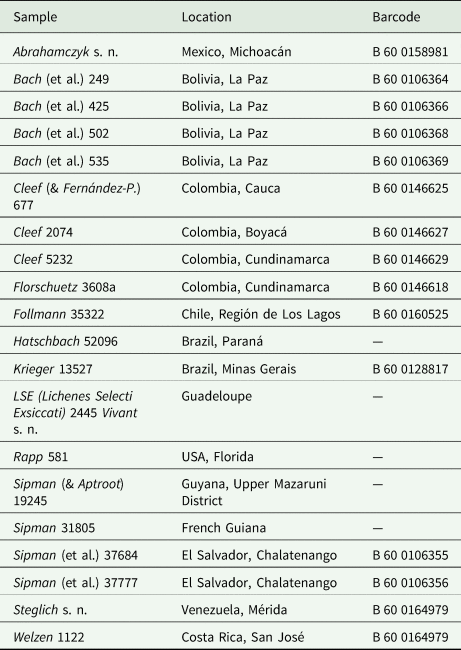
Based on the studies by Lücking et al. (Reference Lücking, Dal-Forno, Sikaroodi, Gillevet, Bungartz, Moncada, Yánez-Ayabaca, Chaves, Coca and Lawrey2014, Reference Lücking, Dal Forno, Moncada, Coca, Vargas-Mendoza, Aptroot, Arias, Besal, Bungartz and Cabrera-Amaya2017), we compiled three data sets of the genus Cora Fr. to illustrate and test PhyloKey: 1) a molecular alignment of the ITS fungal barcoding locus for 87 formally described and sequenced species plus two outgroup species of the genus Corella Vain. (‘alignment’ in fasta format; Supplementary Material File S1, available online); 2) a matrix of 20 characters for the 87 ingroup species (the same as analyzed in Dal Forno et al. (Reference Dal Forno, Lawrey, Moncada, Bungartz, Grube, Schuettpelz and Lücking2022)), divided into one ecological (substratum), 11 phenotype (morphology, anatomy, chemistry; Fig. 1), and eight distributional characters (main distribution areas; ‘reference matrix’ in Phylip format; Table 1, Supplementary Material File S2, available online); and 3) a matrix of the same 20 characters for 398 samples to be identified (‘query matrix’ in Phylip format; Supplementary Material File S3, available online). For the latter, 200 test samples (‘samples’) were generated from the original data matrix by randomly selecting ten out of the 87 species (C. applanata B. Moncada et al., C. caliginosa Holgado et al., C. campestris Dal-Forno et al., C. crispoleslia B. Moncada et al., C. davibogotana Lücking et al., C. dewisanti B. Moncada et al., C. dulcis B. Moncada et al., C. fimbriata L. Y. Vargas et al., C. pichinchensis Paredes et al. and C. soredavidia Dal-Forno et al.), and 20 samples per species were generated by randomly deleting an increasing number of characters, from zero to 19, for each species. This data set was used to assess the effect of incomplete character sampling on the accuracy of species identification. In addition, we randomly selected 20 samples from herbarium collections held in B traditionally identified as Cora pavonia or Dictyonema glabratum (Table 2), to assess whether some of these would match described species and how potentially undescribed species would behave using this approach. We further added all 89 ingroup and outgroup species twice to the data set, once as reference and once for calibration purposes.

Figure 1. Selected characters and character states used to score Cora species and samples. For complete list of characters and states, see Table 1. A, sutures in C. suturifera Nugra et al. B, rugose surface in C. auriculeslia B. Moncada et al. C, narrowly undulate surface in C. celestinoa B. Moncada et al. D, broadly undulate surface in C. imi Lücking et al. E, pitted surface in C. elephas Lücking et al. F, setose upper surface in C. barbifera B. Moncada et al. G, strigose upper surface in C. hirsuta (B. Moncada & Lücking) Moncada & Lücking. H, soredia in C. hawksworthiana Dal-Forno et al. I, viaduct-shaped upper cortex in C. leslactuca Lücking et al. J, paraplectenchymatous upper cortex in Corella melvinii (Chaves et al.) Lücking et al. K, papillae in the lower medulla in Cora haledana Dal-Forno et al. L, adnate hymenophore in C. soredavidia. M, concentric hymenophore in C. viliewoa Lücking et al. N, cyphelloid hymenophore in C. benitoana B. Moncada et al. O, pigment (after rewetting) in C. rubrosanguinea Nugra et al. In colour online.
Table 1. Characters used to score Cora species and samples. For visual character definitions, see Fig. 1, and for additional details on character definitions, see Dal Forno et al. (Reference Dal Forno, Lawrey, Moncada, Bungartz, Grube, Schuettpelz and Lücking2022).

Table 2. Details of herbarium specimens held at B and traditionally identified as Cora pavonia or Dictyonema glabratum, used for the PhyloKey test.
The molecular reference tree was computed from the molecular alignment through a maximum likelihood search with RAxML v. 8.2.8 (Stamatakis Reference Stamatakis2014), with non-parametric bootstrapping using 1000 replicates under a GTRGAMMA model. To test the effect of topology on the performance of the key, we also computed two additional trees. A morphological reference tree was built by subjecting the morphological matrix to a maximum likelihood search, also using RAxML v. 8.2.8 (Stamatakis Reference Stamatakis2014), with non-parametric bootstrapping using 1000 replicates under a MULTIGAMMA model. In addition, a random tree was generated in PAUP v. 4.0 b10 (Swofford Reference Swofford2003). The molecular and morphological reference trees included branch lengths (phylograms), whereas the random tree was used as a simple cladogram (‘reference trees’ in Newick format; Supplementary Material File S4, available online).
Morphology-based phylogenetic binning is a two-step approach, first calculating the character weight vectors, using either maximum likelihood (ML) or maximum parsimony (MP), and then binning the samples to be identified onto the reference tree (Berger et al. Reference Berger, Stamatakis and Lücking2011). For the weight vectors, we ran the vector analysis in RAxML v. 7.2.6 (Stamatakis et al. Reference Stamatakis, Ludwig and Meier2005) relating the matrix (in Phylip format) to each of the reference trees (in Newick format). The command line runs [raxmlHPC.exe -f u -m MULTIGAMMA -s matrix.phy -t reference.tre -n weight_vector.txt] for the ML weight vector and is identical but with upper case U [-f U] for the MP weight vector. In addition, we employed a uniform weight vector and an arbitrary vector weighting character based on their ease of observation and distinctiveness (Table 3). For the latter, we assigned three weights: 100% for characters easy to observe, discrete or unique (e.g. soredia, hymenophore type, distribution in the Palaeotropics); 50% for characters difficult to observe, subtle, or continuous, or for ecological and most chorological characters (e.g. colour, lobe size, substratum); and 75% for characters that we considered intermediate in this respect (Table 3).
Table 3. Character weights used in the different setups to bin the Cora samples onto the reference tree. For ‘even’, all characters were weighted equally. The MP and ML weights were derived from the corresponding weight vector algorithm implemented in RAxML, depending on the underlying reference tree. MP = maximum parsimony, ML = maximum likelihood, Mol = molecular reference tree, Mor = morphological reference tree, Ran = randomized reference tree. Note the differences in character weights between MP and ML approaches and between underlying reference trees.

The matrix of samples to be identified requires inclusion of the species present in the reference tree, so the complete matrix contained 87 (known species) + 2 (outgroup) + 220 (samples) units. The samples were then binned onto each of the three reference trees, with three different weight vectors (even, MP, ML), in RAxML v. 7.2.6, with 1000 bootstrap replicates, using the command line [raxmlHPC.exe -f v -m MULTIGAMMA -a weight_vector.txt -s samples.phy -t reference.tre -n identification.txt -x 12345 -# 1000], which corresponds to the Evolutionary Placement Algorithm (EPA; Berger & Stamatakis Reference Berger and Stamatakis2010; Berger et al. Reference Berger, Stamatakis and Lücking2011). This resulted in a total of nine combinations for the same 220 samples (three reference trees × three weight vectors). In addition, we tested the fourth (arbitrary) weight vector with the random tree.
For each of the randomly selected samples with decreasing number of characters binned and for each reference tree, we computed a combined score across the three weighting schemes as follows:
 $$ \rm S_{Ref} = ( {N_{MP} \times B_{MP} + N_{ML} \times B_{ML} + N_{even} \times B_{even}} ) / 3000, \;$$
where SRef = combined score for each reference tree (molecular, morphological, random), NMP, NML, Neven = number of correctly binned species, and BMP, BML, Beven = mean bootstrap support for correctly binned species using MP, ML, and even weights.
The analytical output from RAxML includes a number of files in text format, two of which were used for visualization (all other output files can be discarded). One is the classification table, a tabular text file named ‘RAxML_classification’, with the node placements of each query taxon and the corresponding bootstrap support values. This text file was adjusted for inspection in a spreadsheet editor, in this case Microsoft Excel, by globally replacing spaces with tabulators (alternatively, the table can be opened in Excel using space as separator). The second file is the classification tree, originally in Newick format, named ‘RAxML_labelledTree’, which can be opened in various tree viewing editors. Here, we used FigTree v. 1.4.4 (Rambaut Reference Rambaut2018), for which the output file had to be adjusted as follows prior to opening: 1) globally replacing the string ‘:1.0[’ with ‘[’ and then ‘]’ with ‘]:1.0’ (which switched the order of branch length and node ID labels); 2) checking instances of identical terminal output names (which can occur as the bootstrap support values are added to the query names and alternative placements can have identical support). Such instances were then made unique by adding the suffix letters ‘a’, ‘b’, etc.
Results
For the ‘simulated’ samples, the three different reference tree approaches resulted in overall similar outcomes in the individual results (Table 4; Supplementary Material File S5, available online) and the combined score (Fig. 2). In all three cases, samples with complete character sets were placed correctly, with a placement-support score (PSS) of 1.00 for the molecular and morphological reference trees and 0.99 for the random tree. Performance in terms of correct placement declined with increasing number of missing characters but resulted in very high PPS (0.95 or higher) down to three missing characters for the molecular and random trees, and high PPS (0.70 or higher) down to ten missing characters for the molecular tree, four missing characters for the morphological tree, and eight missing characters for the random tree. The threshold of 0.50 PPS was reached for all trees at ten missing characters, followed by a strong drop in performance, and 15 or more missing characters resulted in a PPS of close to zero in all three approaches. The molecular reference tree performed best overall, followed by the random and the morphological reference trees. The random reference tree performed most consistently (Fig. 3), with the least amount of variation as a function of increasing number of missing characters, whereas both the molecular and the morphological trees had positive and negative spikes for particular proportions of missing characters (Fig. 2).
Table 4. Results of the ‘simulated’ Cora test samples with increasing number of missing characters. MP = maximum parsimony; ML = maximum likelihood.


Figure 2. Performance of the combined score (number of matches and mean bootstrap support) relative to the nature of the reference tree for Cora samples with decreasing number of sampled characters (e.g. minus_01 means one less character out of the 20 scored and so forth, while minus_19 means only one character was used). In colour online.

Figure 3. Labelled classification tree resulting from phylogenetic binning of the simulated Cora samples onto the random reference tree under an even weighting scheme. Blue species names = correctly binned samples with decreasing number of randomly sampled characters; orange filled circles= incorrectly binned samples with low number of randomly sampled characters with ≥ 70% bootstrap support. For detailed tree, see Supplementary Material File S7 (available online). In colour online.
For the molecular reference tree, even and maximum likelihood (ML) weighting performed better than maximum parsimony (MP) weighting, both with nine out of ten correct placements with as many as ten missing characters; however, MP weighting was more consistent, with both even and ML weighting showing positive and negative spikes. The morphological reference tree showed a similar result between all three weighting approaches, whereas with the random tree, even weighting outperformed both MP and ML weighting (Table 4).
The test with herbarium samples, including all known species with a full character set each for calibration, placed the 89 known species correctly using even character weights, with 99.1% average bootstrap support; out of these, 80 species were placed correctly with 100% support, 85 species with ≥ 95%, and two species (Cora squamiformis Wilk et al. and C. terricoleslia Wilk et al.) with < 70% (Supplementary Material File S5). Using maximum parsimony (MP) weights, 88 species were placed correctly, with an average support of 97.8%; of these, 54 had 100% support and 74 had > 95% (none below 70%). Under maximum likelihood (ML) weighting, all 89 species were placed correctly, with an average of 96.6% support; 79 had 100% support, 81 had ≥ 95%, and three < 70% (Supplementary Material File S5). Thus, overall performance was best with even weights (96% of species placed correctly with 95% support or higher), followed by ML weighting (91% of species) and MP weighting (83% of species).
Using the above results as expectation values for the outcome with the 20 herbarium samples, the latter were placed 50 times (out of a possible 60) with a known species: 17 times (out of 20) using even weight, with 90.8% average support, 15 times (out of 20) using MP weight, with 92.1% average support, and 18 times (out of 20) using ML weight (Supplementary Material File S6, available online), with 88.7% average support (Supplementary Material File S5). Based on expectation value from calibration with the known species, seven samples each were classified as ‘no match’ under even and MP weighting (more than 1% point difference with the expected value for the best scoring result), whereas under ML, ten samples were classified as ‘no match’; for even weighting, ‘no match’ results varied between 94.3% and 56.1% support, for MP between 95.2% and 63.1%, and for ML between 94.7% and 50.7% (Supplementary Material File S5). Five out of the 20 samples were placed with a single species; of these, two included two internal node placements (unresolved) and one (Steglich s. n. from Venezuela) included one internal node placement (under MP weights), otherwise being placed with C. dalehana B. Moncada et al. from Colombia.
Samples Sipman 37684 and Sipman 37777 (both from El Salvador and with identical characters) were the only ones placed three times (i.e. with each different weighting method) with the same known species (C. barbulata Lücking et al. from Costa Rica); they differ, however, in a few characters and do not represent that species but an undescribed taxon close to it. Nine further samples were placed with two different known species depending on the weighting approach; in five of these, additional placement at an unresolved, internal node was observed (three of these under MP weights). The remaining six samples were each placed with three different known species under each of the weighting approaches (Supplementary Material File S6).
Comparison of the character scores of the 20 herbarium samples revealed that two were conspecific with known species, namely a sample from southern Colombia (Cleef 677) with Cora cuzcoensis Holgado et al. from Peru, and a sample from Venezuela (Steglich s. n.) with C. dalehana from central Colombia. The remaining 18 samples represented presumably undescribed species; the number of ecological and morphological characters in which each of them differed from the most similar, known species, varied between one (three samples), two (five samples), three (eight samples), and four (two samples), out of 12 (not counting the eight distribution characters).
Discussion
We introduced and tested PhyloKey, a novel method for batch-identification of specimens based on an underlying phenotype character matrix. PhyloKey is based on the approach of phenotype-based phylogenetic binning (Berger & Stamatakis Reference Berger and Stamatakis2010; Berger et al. Reference Berger, Stamatakis and Lücking2011), a tool used in integrative taxonomy of fungi (lichens), plants and animals to quantitatively integrate phenotype data with molecular phylogenies (Koch et al. Reference Koch, Kiefer, German, Al-Shehbaz, Franzke, Mummenhoff and Schmickl2012; Parnmen et al. Reference Parnmen, Lücking and Lumbsch2012; Rivas Plata et al. Reference Rivas Plata, Lücking and Lumbsch2012; Lücking et al. Reference Lücking, Mangold, Rivas Plata, Parnmen, Kraichak and Lumbsch2015b; Dohrmann et al. Reference Dohrmann, Kelley, Kelly, Pisera, Hooper and Reiswig2017; Buitrago et al. Reference Buitrago, MacDougal and Coca2018; Lücking & Kalb Reference Lücking and Kalb2018; Perlmutter et al. Reference Perlmutter, Rivas Plata, LaGreca, Aptroot, Lücking, Tehler and Ertz2020; Badano et al. Reference Badano, Fratini, Maugeri, Palermo, Pieroni, Cedola, Haug, Weiterschan, Velten and Mei2021; Černý & Natale Reference Černý and Natale2022). In contrast to interactive keys, such as DELTA (Dallwitz et al. Reference Dallwitz, Paine and Zurcher2006), Xper2 (Ung et al. Reference Ung, Dubus, Zaragüeta-Bagils and Vignes-Lebbe2010) or Dryades KeyToNature (Nimis et al. Reference Nimis, Riccamboni and Martellos2012; Nimis & Martellos Reference Nimis and Martellos2020), PhyloKey allows evaluation of identification results by means of bootstrap support values, thus providing a measure of reliability for individual placements, given all possible alternatives. An additional advantage of PhyloKey is the possibility to simultaneously bin a large number of previously scored specimens.
PhyloKey is comparable to other interactive identification tools in providing multi-access entry. However, in contrast to interactive keys, characters are not entered subsequently, not forcing the user to decide on the sequence of characters (in some tools, such as DELTA, guided by the identification process). In PhyloKey, all scored characters are evaluated simultaneously. Bootstrapping then reconstructs placements based on character subsets, thus assessing internal consistency of the sampled characters. Our test showed that using a molecular reference tree, specimens were mostly binned correctly and with support, with as little as ten out of 20 characters. For the random reference tree, the minimum number of characters required to bin most specimens correctly and with support was 12–14, and for the morphological reference tree was 16. Thus, scoring at least 70% of the characters resulted in correct binning with support in most cases under the various reference trees and weighting schemes. Surprisingly, even weighting performed consistently equal to or better than MP weighting and both methods performed better than ML weighting, consistent with the results of the binning approach by Berger et al. (Reference Berger, Stamatakis and Lücking2011) on the genera Allographa and Graphis, where MP was also found to outperform ML weighting. This is probably due to the nature of the underlying phenotype characters, which can hardly be forced into an evolutionary model and so the ML weighting approach is less intuitive than MP weighting.
Compared to a traditional dichotomous (single-access) key, PhyloKey requires a set of characters to be scored for each species to be identified, not knowing a priori which characters will eventually be critical for the identification. A traditional dichotomous key will instead guide the user to observe specific characters, limited to those considered diagnostic at each step of the identification process. For instance, if a genus contains a single species with a unique pigment, in a dichotomous key that species will be easily keyed out first using just that one character. The time to observe all characters to establish a matrix is therefore longer when using PhyloKey, typically about twice as long (i.e. the mean time one would arrive at a species in the middle of a dichotomous key). For example, in the dichotomous key to Cora provided by Lücking et al. (Reference Lücking, Dal-Forno, Lawrey, Bungartz, Rojas, Marcelli, Moncada, Morales, Nelsen and Salcedo2013), arriving at each species keyed out there would require the observation of between three and eight morpho-anatomical characters, on average about five. To use PhyloKey, about ten characters would have to be scored per specimen, not counting chorological characters (distribution), requiring about ten minutes per specimen (one minute per character). However, this increased amount of time is compensated in PhyloKey by the simultaneous identification of many specimens in batch mode. While the computation only takes seconds, running each specimen through a dichotomous key might typically require around five minutes. Therefore, for ten specimens, the total identification time using a dichotomous key would amount to 50 min (scoring of 5 characters each on average, at 1 min per character) + 50 min (average working time going with each specimen through the key) = 100 min, whereas in PhyloKey it would take 100 min (complete matrix scoring) + 0 min (key), so about the same time. Thus, on average, the advantages and disadvantages of both approaches regarding time balance each other out, with the difference that a matrix-based approach adds value by generating a lasting data set. Generally, a dichotomous key would work faster if the group in question is well known and has easily perceived diagnostic characters, whereas PhyloKey provides an advantage when the group in question is not well known (i.e. undescribed species are to be expected) and diagnostic characters are subtle. For instance, in the above example of a uniquely pigmented species within a genus, a dichotomous key would identify that species correctly only if it is indeed the only species with that character. If at least one other, unrecognized species with the same character existed, a dichotomous key would not alert the user to that possibility and since no other characters are used at that position in the key, the user may not be aware of potential deviations. In PhyloKey, as well as in other matrix-based identification tools such as DELTA Intkey, the resulting identity scores will tell the user whether there is a perfect match or whether there are deviations in one or more characters. A further, unique advantage of PhyloKey is found in obtaining a placement support value for each sample.
Character scoring in PhyloKey is no different to a scoring scheme required for an interactive multi-access key, such as DELTA Intkey, and so, apart from compatibility of import/export formats, no additional work is needed when implementing PhyloKey on a set of data originally prepared to be used in an interactive key. The required data matrices are not only interchangeable but can be used for many other downstream analyses, such as multivariate techniques or ancestral character state analysis on a phylogenetic reference tree (e.g. Parnmen et al. Reference Parnmen, Lücking and Lumbsch2012). Comprehensive character scoring also forces the user to perform comparative observations, making the scoring process more objective and reliable, whereas dichotomous keys rely on ad hoc observations. One advantage of interactive keys over PhyloKey is that the evaluation of individual characters is transparent during the identification process and can be accompanied by guiding illustrations or imagery, such as in Dryades KeyToNature (Nimis et al. Reference Nimis, Riccamboni and Martellos2012; Nimis & Martellos Reference Nimis and Martellos2020). This possibility may be more attractive to users who are not familiar with the diagnostic characters of a group in question. However, the scoring process in PhyloKey can also be accompanied by character illustrations, especially when set up for particular groups, as shown in the Material and Methods section above (Fig. 1).
One surprising result of our analysis was the good performance of the randomized reference tree. Normally, the binning method, and hence PhyloKey, would rely on a molecular reference tree to guarantee the best possible placement of a specimen or taxon based on phenotype data, due to the character weighting process. In lieu of a molecular reference tree (e.g. when only a small number of taxa within the target group have molecular data), a tree based on the phenotype characters seemed a viable alternative. However, in our analysis, such a morphological reference tree performed less well, probably because its internal topology is based on exactly the same characters that are being used for the binning process. A randomized tree avoids this shortcoming and seems to have no negative effects on correct placement of individual taxa or specimens compared to a molecular reference tree, probably because the underlying relationships between taxa (backbone) do not affect the closest binning match. This finding offers a more universal use of the PhyloKey approach, by simply establishing a randomized reference tree when sufficient sequence data for a molecular reference tree are not available. We hypothesize that a randomized reference tree will work well if most of the species in a group, or at least the range of phenotypic variation of the group, are known and represented by the reference terminals; whereas a phenotype-based reference tree has the potential for better predictive placement of specimens representing unknown taxa, as placements also reflect the character composition of deeper nodes.
Looking at the performance of PhyloKey relative to previously unidentified herbarium samples, presumably undescribed species obtained different placements under each weighting approach (including internal nodes), in each case with at least one strongly supported ‘mismatch’, that is, suggesting a known species as the result with 1% difference or less from the expected value. The only exceptions were the two samples Sipman 37684 and Sipman 37777, consistently placed with a single species (C. barbulata) but differing in three ecological and morphological characters, including the diagnostic medullary papillae. On the other hand, the two samples that presumably represented known species behaved differently. Sample Steglich s. n., representing C. dalehana, was placed twice with that species, under even and ML weights, whereas MP weighting placed the sample on an internal node. The sample deviated from C. dalehana in a single score, for the character ‘sutures’, scored as ‘1’ (short) in C. dalehana and ‘0’ (absent) in the sample, which we consider an ‘allowable’ deviation, as the sample was not sufficiently well developed. The deviation did not affect its inferred placement under even and ML weights but apparently did under MP weighting. In contrast, sample Cleef 677 (corresponding to C. cuzcoensis) was placed correctly under an even weighting scheme, on an internal node under ML weight, and incorrectly under MP weight. While this sample agreed with C. cuzcoensis in all ecological and morphological characters, it differed in the distribution grid (northern versus central Andes), which was included in the PhyloKey matrix and apparently caused the partially inconsistent placement. However, in both samples, even weighting was not sensitive to these scoring particularities and placed both correctly, whereas ML weighting resulted in one correct and one unresolved placement and MP weighting in one unresolved and one incorrect placement. In these cases, the PhyloKey approach makes the establishment of potentially new species more reliable, by simultaneously identifying their closest matches and hence avoiding overlooking potentially available names elsewhere, and also by allowing identification of the quantity and quality of character mismatches. In that sense, PhyloKey could not only be used as an identification tool but also as a quantitative tool to recognize potential new species, simultaneously highlighting the most similar known taxa and the number of differences to these. PhyloKey could therefore be a useful tool in ‘non-molecular museomics’, the quantitative assessment of phenotype characters and their integration with molecular data, by scoring a large number of herbarium samples and evaluating their placement on a reference tree. While DNA barcoding of older herbarium samples is partially feasible and has been shown to work in Cora (Dal Forno et al. Reference Dal Forno, Lawrey, Moncada, Bungartz, Grube, Schuettpelz and Lücking2022), it depends on the condition of the underlying sample and is often unsuccessful, so PhyloKey could be a non-molecular complement to this approach.
It should be noted that the phenotype-based phylogenetic binning approach provides an objective method to predict the phylogenetic placement of individuals in the absence of DNA sequence data; however, this prediction may not be accurate and depends on the number of taxa already sequenced and the phylogenetic signal of the scored characters. Usually, accuracy is obtained at genus or within-genus clade level, but not necessarily identifying the closest relative at species level (e.g. Berger et al. Reference Berger, Stamatakis and Lücking2011; Perlmutter et al. Reference Perlmutter, Rivas Plata, LaGreca, Aptroot, Lücking, Tehler and Ertz2020). One herbarium specimen tested here, Rapp 581 from the USA (Florida), recently described as Cora timucua Dal Forno et al. (Lücking et al. Reference Lücking, Kaminsky, Perlmutter, Lawrey and Dal2020c), showed slight differences in its placement when based on phenotype data versus DNA sequence data (Lücking et al. Reference Lücking, Kaminsky, Perlmutter, Lawrey and Dal2020c). Fortunately, the exact phylogenetic placement of an individual is of secondary importance in the PhyloKey application: as we could show, individuals are generally placed correctly if a matching taxon is already in the reference matrix, whereas the recognition of potentially novel taxa does not depend on their precise phylogenetic placement.
How to implement PhyloKey
The PhyloKey approach requires the following tools:
• a spreadsheet tool (Excel, Numbers, or similar)
• a text editor (Word, Editor, Wordpad, Notepad, Pages, BBEdit, or similar)
• RAxML (tested versions: 7.2.6, 8.2.0)
• tree viewing software (tested: FigTree v.1.4.4, see below).
The following data sets need to be established:
• a phylogenetic reference tree of a set of known taxa in Newick format (e.g. Supplementary Material File S4, available online); it can be based on actual molecular data (e.g. Supplementary File S1) or on phenotype data (e.g. Supplementary Material File S2) or can be assembled manually as a simple tree format assuming underlying ‘relationships’; the tree can contain branch lengths but these are not required
• a reference matrix of (diagnostically important) phenotype characters for the same taxa (terminals) used for the reference tree, with exactly the same names; the matrix can be established in a spreadsheet but must be converted into Phylip format prior to analysis (e.g. Supplementary Material File S2); note that unknown or missing data can be expressed using a ‘?’ sign
• a matrix of (diagnostically important) phenotype characters for a set of query specimens, in exactly the same format as the reference matrix; the matrix can be established in a spreadsheet but must be converted into Phylip format prior to analysis (e.g. Supplementary Material File S3); note that unknown or missing data can be expressed using a ‘?’ sign
The approach is implemented via the following steps:
-
Step 1. Computation of the weight vector(s) for the phenotype characters based on their distribution over the reference tree, either based on maximum parsimony (MP) or maximum likelihood (ML) or both; this is invoked in RAxML (e.g. v. 7.2.6) using the following command line (alternatively as Windows batch file ‘.bat’):
• raxmlHPC.exe -f U -m MULTIGAMMA -s matrix.phy -t reference.tre -n weight_vector_MP.txt (for the MP weight vector)
• raxmlHPC.exe -f u -m MULTIGAMMA -s matrix.phy -t reference.tre -n weight_vector_ML.txt (for the ML weight vector)
where -f u (-f U) = algorithm, -m MULTIGAMMA = underlying evolutionary model, -s matrix.phy = matrix selection (matrix.phy = reference matrix in Phylip format), -t reference.tre = tree selection (reference.tre = reference tree in Newick format), and weight_vector_MP.txt/weight_vector_ML.txt = output of the weight vector (text format, a series of numbers between 0 and 100).
-
Step 2. Running the binning analysis; this is invoked in RAxML (e.g. v. 7.2.6) using the following command line (alternatively as Windows batch file ‘.bat’):
• raxmlHPC.exe -f v -m MULTIGAMMA -a weight_vector_ML.txt -s samples.phy -t reference.tre -n identification.txt -x 12345 -# 1000
where -f v = algorithm, -m MULTIGAMMA = underlying evolutionary model, -a weight_vector_ML.txt = selection of the weight vector, -s samples.phy = query matrix selection (samples.phy = query matrix of all samples to be analyzed, in Phylip format), -t reference.tre = tree selection (reference.tre = reference tree in Newick format), -n identification.txt = name designation for the various output files, -x 12345 = random number seed, and -# 1000 = number of bootstrap pseudoreplicates.
-
Step 3. Visualizing the classification table; open the output file named ‘RAxML_classification[…].txt’ in a text editor and globally replace spaces with tabulators, then save and open with a spreadsheet editor, such as Microsoft Excel (alternatively, open original file in spreadsheet editor using space as separator). The table will display four columns: 1) sample name, 2) node ID of nearest placement, 3) bootstrap support value for placement (number of bootstrap replicates), and 4) branch length of the original reference tree for that node; edit classification table as desired (e.g. Supplementary Material File S5).
-
Step 4. Visualizing the classification tree (e.g. in FigTree); open the output file named ‘RAxML_labelledTree[…].txt’ in a text editor; globally replacing the string ‘:1.0[’ with ‘[’ and then ‘]’ with ‘]:1.0’ (which switched the order of branch length and node ID labels); check instances of identical terminal output names and make them unique by adding the suffix letters ‘a’, ‘b’, etc.; open adjusted tree file in tree viewer (e.g. FigTree) and edit as desired, then export as PDF (e.g. Supplementary Material File S6).
-
Step 5. If desired, the taxonomic identities of the node labels in the output tree can be added to the classification table (e.g. Supplementary Material File S5 worksheet ‘Herbarium’).
-
Step 6. If desired, the original phenotype characters can be added to each query and ID label in the classification table, to assess the corresponding matching level (e.g. Supplementary Material File S5 worksheet ‘Herbarium’).
Acknowledgements
Harrie Sipman is thanked for his assistance in selecting the herbarium specimens tested here. MDF would like to acknowledge funding from NSF (PRFB 1609022) and the Smithsonian Institution (NMNH Peter Buck Postdoctoral Fellowship).
Author ORCIDS
Robert Lücking, 0000-0002-3431-4636; Bibiana Moncada, 0000-0001-9984-2918; Manuela Dal Forno, 0000-0003-1838-1676.
Supplementary Material
The supplementary material for this article can be found at https://doi.org/10.1017/S0024282923000415.


 Open access