Experimental setup

The experiments were performed at the CIRCE beamline of the ALBA Synchrotron Light Source.^{Reference Aballe, Foerster, Pellegrin, Nicolas and Ferrer18} A schematic plot of the measurement is shown in Figure 1. We fabricated hybrid devices made of micrometer-scale magnetic structures of nickel (Ni) on piezoelectric LiNbO₃ substrates. An oscillating electric field applied to interdigital transducers (IDTs) generates SAWs that propagate through the surface of the piezoelectric substrate. Devices were designed to produce SAWs at a frequency matching the repetition rate of the x-ray pulses of the ALBA Synchrotron (f _SAW = 499.654 MHz). We phase locked the excitation signal of the SAWs to the master clock of the synchrotron and, thus, the x-ray pulses. Consequently, fixed phase images of the SAWs are achieved through photoelectrons emitted from many x-ray light pulses (typically 500 million [i.e., 1 s exposure time]) illuminating the sample.^{Reference Foerster, Prat, Massana, Gonzalez, Fontsere, Molas, Matilla, Pellegrin and Aballe19}

Figure 1. Schematic plot of the experimental setup. X-rays (blue) with different circular polarization illuminate the sample with a repetition rate of f ₀ ∼ 500 MHz (20 ps pulse length). A radio-frequency (RF) electric signal is sent to the interdigital transducer (IDT, [yellow]) having the same frequency as the synchrotron repetition rate. The IDT generates a piezoelectric surface acoustic wave (SAW) that propagates through the LiNbO₃ substrate (gray) and interacts with the magnetic nanostructures (red) deposited on the acoustic path. The phase-resolved variation of the piezoelectric voltage at the surface sample is probed with the photoemission electron microscope (PEEM) (upper left image), as well as the magnetic contrast (upper right image) along the x-ray propagation direction arising from the x-ray magnetic circular dichroism (XMCD) effect.

Stroboscopic photoemission electron microscope (PEEM) images were recorded for each phase delay between the SAW and the x-ray pulses, providing magnetic contrast of the sample surface through the x-ray magnetic circular dichroism (XMCD) effect. These stroboscopic measurements allowed us to reconstruct the strain-wave propagation and the effect on magnetic nanostructures with a time resolution of ∼80 ps. Magnetic structures of Ni (20 nm in thickness) were defined with electron-beam lithography and deposited by electron-beam evaporation into the SAW path (Figure 1). Further details on sample fabrication and the experimental setup can be found in References Reference Foerster, Macià, Statuto, Finizio, Hernández-Mínguez, Lendínez, Santos, Fontcuberta, Hernàndez, Klaeui and Aballe17 and Reference Foerster, Prat, Massana, Gonzalez, Fontsere, Molas, Matilla, Pellegrin and Aballe19.

Dynamic measurements of strain

Before turning to the magnetic response, we first address the methodology used to (1) quantify the strain amplitude induced by the SAW and (2) determine the local SAW phase in a given image. The piezoelectric voltage associated with the SAW shifts the energy of the secondary electrons that leave the sample surface, producing a visible contrast in PEEM images. In Figure 2a–b,^{Reference Foerster, Macià, Statuto, Finizio, Hernández-Mínguez, Lendínez, Santos, Fontcuberta, Hernàndez, Klaeui and Aballe17} we show direct x-ray PEEM images of a synchronized 500 MHz SAW measured under the pulsed synchrotron x-ray illumination, with an integration time of 10 s. We can see a clear contrast with a periodicity matching the wavelength of the SAW (λ = 8 μm), which is independent of x-ray photon energy or polarization. The image contrast depends strongly on the sample bias voltage, –3 V in Figure 2a and 0.5 V in Figure 2b. In the absence of any further electrical field (e.g., due to the SAW, or sample charging), the bias voltage would correspond to the secondary electron kinetic energy used to form the image. In summary, the contrast between the two images at different bias voltages has fully inverted. Scanning the bias voltage allows for a gradual change of the contrast and by focusing on particular sample positions corresponding to different SAW phases—or different strain states—we can obtain local kinetic energy spectra of the secondary electrons (photoemission intensity).^{Reference Foerster, Macià, Statuto, Finizio, Hernández-Mínguez, Lendínez, Santos, Fontcuberta, Hernàndez, Klaeui and Aballe17}

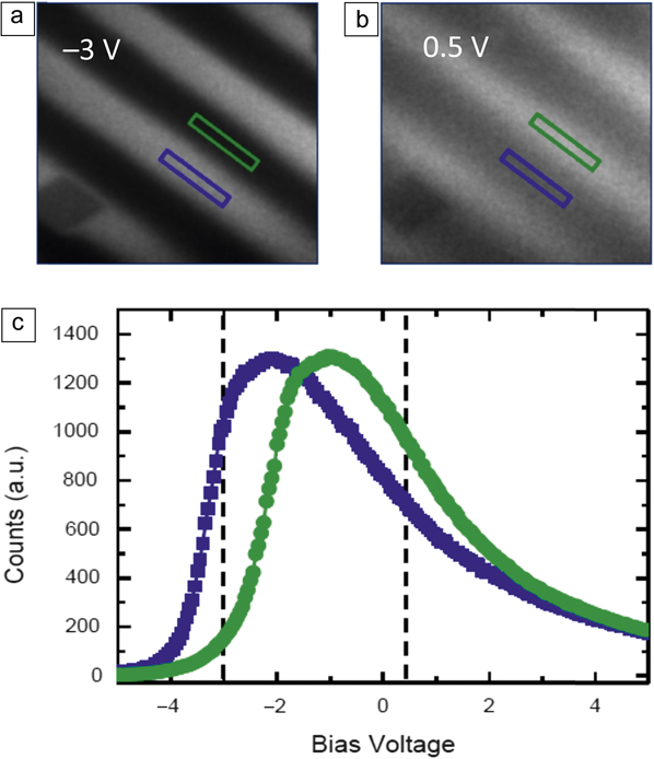
Figure 2. X-ray photoemission electron microscope images of a surface acoustic wave (SAW) at sample bias of (a) –3 V and (b) +0.5 V. The photon energy 848 eV, the total exposure time (10 s), and the size ≈ 30 × 23 μm² are the same for both. The SAWs produce a contrast in the images because of the piezoelectric voltage associated with the wave. In the lower left and upper right corner of the images, the same alignment markers are visible as dark squares. (c) Local photoelectron bias voltage scans for the centers of the different stripes. The vertical lines mark the conditions at which the images in (a–b) were recorded. The maximum shift between local spectra shown in (c) allows for a quantification of the strain associated with the SAW. Green and blue rectangles indicate the regions of the sample where the local spectra shown in (c) were extracted.^{Reference Foerster, Macià, Statuto, Finizio, Hernández-Mínguez, Lendínez, Santos, Fontcuberta, Hernàndez, Klaeui and Aballe17}

Figure 2c shows local spectra as a function of the sample bias voltage, for two surface region areas corresponding to opposite phases of the SAW,^{Reference Foerster, Macià, Statuto, Finizio, Hernández-Mínguez, Lendínez, Santos, Fontcuberta, Hernàndez, Klaeui and Aballe17} marked with blue and green rectangles in Figure 2a–b. The vertical lines mark the conditions in which Figure 2a (left line) and Figure 2b (right line) were recorded. The spectral shift from the blue and green positions of the sample explains the contrast inversion in Figure 2a–b. Since all parameters (photon flux and SAW power) except for the bias voltage are the same over the imaged area, we ascribe the shift of the photoelectron emission spectrum to the local piezoelectric surface potential accompanying the strain wave, which is approximately 1.2 V in Figure 2c. This value can be determined either from the corresponding maximum position or the position of the maximum slope. The electric amplitude (maximum shift between local spectra in Figure 2c) of the surface electric potential associated with the SAW can be converted into strain amplitudes acting on the Ni nanostructures by numerically solving the coupled differential equations of the mechanical and electrical displacement for an acoustic propagating wave.^{Reference Auld20,Reference Lewis, Ash and Paige21}

Dynamic measurements of acoustomagnetic modes

We now turn to the measurements of the magnetic response of the Ni patterns. PEEM images taken with opposite circular x-ray photon helicities are subtracted to image the local magnetization through the dichroic effect (XMCD). The gray scale intensity of the resulting XMCD images is proportional to the Ni magnetization along the x-ray incidence direction. In order to quantify the magnetic anisotropy induced by the SAW strain through the magnetoelastic effect, polycrystalline Ni squares with 2 × 2-µm^{Reference Locatelli, Cros and Grollier2} size and 20-nm thickness with four magnetic domains in a flux closure configuration are considered. This configuration, known as Landau flux-closure state (Figure 3), represents an equilibrium state with a corresponding energy minima and a restoring force with respect to excitations.

Figure 3. Simultaneous images of piezoelectric voltage and magnetization. (a–b) Photoemission electron microscope shows the piezoelectric voltage. Dashed blue lines illustrate the strain wave. (c–d) X-ray magnetic circular dichroism–photoemission electron microscope images show the magnetic configuration. Images of 2 × 2 µm^{Reference Locatelli, Cros and Grollier2} Ni squares and are taken at opposite phases of the surface acoustic wave (SAW). The images correspond to maximum and minimum magnetic anisotropy values at 30° and 210°, respectively. The simple comparison with (a) and (b) where the square is not centered in white/black zone already permits visualizing the delay. Solid blue lines guide the eye to the different domains. (e–f) Schematic plots of the effect of SAW on Ni squares for maximal values of strain associated with the SAW. White and black arrows indicate the direction of magnetization. (g) Analysis of the domain configuration from multiple Ni squares as a function of the phase with respect to the SAW. The combined area of black (B) and white (W) domains (amount of magnetization along the x-ray incidence direction) as a fraction of the total square is shown. The best fit to the data with a sinusoidal function is plotted in red. A phase delay of 48° with respect to the strain wave is obtained. A schematic strain wave (without any delay) is plotted in gray in order to highlight the phase difference of the magnetic response. The green dashed horizontal line shows the averaged value without strain, which indicates some residual Ni anisotropy from the deposition process. Note: τ, phase delay.^{Reference Foerster, Macià, Statuto, Finizio, Hernández-Mínguez, Lendínez, Santos, Fontcuberta, Hernàndez, Klaeui and Aballe17}

Initially, we studied Ni squares with sides aligned with the SAW propagation direction. Figure 3a–b shows direct PEEM images at two opposite phases of SAW (corresponding to maximum and minimum magnetic anisotropy values). XMCD-PEEM images of the magnetic domain configuration at the same phase of the SAW are plotted (Figure 3c–d) below the PEEM images. The dashed blue lines in Figure 3a–b plot the strain wave, showing it does not correspond to maximal states; there is a delay between strain and magnetization states. Gray domains (magnetization perpendicular to the SAW propagation direction) are favored in the Figure 3c image, whereas black and white domains (magnetization aligned with the SAW propagation direction) dominate in Figure 3d. Blue lines in Figure 3c–d serve as guide to the eye to indicate the different domains. Schematic plots of the expected magnetization configurations for minimum and maximum strain are shown in Figure 3e–f, respectively, with arrows indicating the direction of magnetization.

The response to SAWs of domain configurations from multiple squares is analyzed by acquiring images at different phase delays between SAW and x-ray pulses. The area occupied by black and white domains in each square is measured at each SAW phase. This area corresponds to the total area with magnetization oriented along the x direction. Figure 3g summarizes the measured values as a function of the SAW phase from multiple squares. Data are fitted by a sinusoidal function (red curve) with the same periodicity as the strain (gray shadowed curve), but with a considerable delay of ∼270 ps (phase delay of ∼48°).

Variations in the magnetic-domain configuration can be converted into variations in magnetic anisotropy by comparison with micromagnetic simulations. The magnetic configurations shown in Figure 3a–b are well reproduced by strain-induced modulation of the magnetic anisotropy K with an amplitude K _SAW ∼ 1 kJm^–3 superimposed on a preexisting, constant uniaxial anisotropy of K _U ∼ 1.2 kJm^–3, most likely from the deposition process by thermal evaporation (shown as a dashed line at 0.67 in Figure 3g). With an estimated in-plane strain of ε_xx = 4.5 × 10^–4 from the measured electric amplitude (Figure 2), we obtain a value for the ratio between the variation of magnetic anisotropy and strain amplitude β = K _SAW /ε_xx = 2.2 × 10⁶ J/m³ at 500 MHz, which is similar to the reported values for static strain^{Reference Finizio, Foerster, Buzzi, Krüger, Jourdan, Vaz, Hockel, Miyawaki, Tkach, Valencia, Kronast, Carman, Nolting and Kläui9} and thus demonstrates the full efficiency of the magnetoelastic effect on this fast time scale.

Next, a different geometry where the Ni squares were rotated by 45° with respect to the SAW propagation direction was explored in order to understand the origin of the observed delay between SAW and magnetization dynamics.^{Reference Foerster, Macià, Statuto, Finizio, Hernández-Mínguez, Lendínez, Santos, Fontcuberta, Hernàndez, Klaeui and Aballe17} The studied configuration was chosen such that the effect of the strain associated with the SAW produces a variation in the magnetization direction within each magnetic domain, but not in their size, because all four magnetic domains are energetically equivalent with respect to the in-plane uniaxial anisotropy induced by the SAW. Thus, no domain growth (or shrinking) through domain-wall displacement occurs. Instead, the magnetization within each of the domains (see schematic plot in Figure 4b) rotates coherently, resulting in a measurable difference of the XMCD intensity levels of the gray domains. The experimental study of this second configuration revealed a much faster magnetic response, showing a sizable decrease in the delay between the SAW strain and the magnetization response, from 270 ps down to about 90 ps (phase delay of ∼16°), being close to the experimental time resolution of 80 ps.^{Reference Foerster, Macià, Statuto, Finizio, Hernández-Mínguez, Lendínez, Santos, Fontcuberta, Hernàndez, Klaeui and Aballe17}

Figure 4. Micromagnetic modeling of the magnetic response in Ni squares caused by a surface acoustic wave (SAW). Amplitude (upper panel) and phase (lower panels) of the magnetic response of a system of 2 × 2 μm² nickel square to an oscillating spatially varying anisotropy as a function of the excitation frequency. Two configurations are shown. (a) Squares are aligned with SAW and (b) squares are tilted 45° with respect to the SAW propagation direction (red arrow). Black and white arrows indicate the magnetization direction of the domains. The same quantities analyzed for the experimental data are plotted in (a) the variation (in %) of the fraction area of black (B) and white (W) domains and in (b), the variation (in %) of the normalized difference between the x-ray magnetic circular dichroism gray intensities between the left and right gray domains, labeled G1 and G2. Different resonances are found, corresponding to the gyration of the central vortex, the motion of domain walls (only in the aligned configuration), and the magnetization rotation within the domains (stronger in the tilted configuration). Dashed lines (in black) mark the frequency f = 500 MHz and the corresponding delay obtained in the phase for both configurations.^{Reference Foerster, Macià, Statuto, Finizio, Hernández-Mínguez, Lendínez, Santos, Fontcuberta, Hernàndez, Klaeui and Aballe17}

Micromagnetic simulations were performed to model the dynamic anisotropy variations caused by the SAW in the Ni nanostructures.^{Reference Foerster, Macià, Statuto, Finizio, Hernández-Mínguez, Lendínez, Santos, Fontcuberta, Hernàndez, Klaeui and Aballe17} The model implements a dynamic variation of the anisotropy in the Ni nanostructures at different frequencies, but with fixed spatial variation of 8 μm, which is the wavelength of the SAW in the experiment. Three different magnetic resonance processes can be identified upon varying uniaxial anisotropy in the studied magnetic nanostructures, which correspond to (1) precessional motion of the magnetization within the magnetic domains, at ∼2 GHz (i.e., FMR like), (2) domain-wall resonance, at ∼500 MHz, as observed in our experiment, and (3) vortex core gyration, at ∼50 MHz.^{Reference van Waeyenberge, Puzic, Stoll, Chou, Tyliszczak, Hertel, Fähnle, Brückl, Rott, Reiss, Neudecker, Weiss, Back and Schütz22} While the first and last are far off the SAW excitation frequency, the second is close to it. In general terms, the investigated system shows the characteristics of a driven oscillator—at frequencies below the resonance, the magnetization configuration follows the changes in anisotropy induced by SAWs without significant delay. Close to resonance, the system follows the anisotropy changes with an increased amplitude and a delay of approximately 90°. At higher frequencies, the system cannot follow the rapid excitation, and the oscillation amplitude of the magnetization vanishes with large delays approaching 180°. We note here that only in the first configuration (squares aligned with SAW) the domain-wall resonance (2) occurs with a resonance frequency close to the SAW excitation frequency, which explains the measured delay in the first configuration.

Figure 4 shows a plot of the phase (lower panels) and amplitude (upper panels) for the two different quantities^{Reference Foerster, Macià, Statuto, Finizio, Hernández-Mínguez, Lendínez, Santos, Fontcuberta, Hernàndez, Klaeui and Aballe17} measured in the experiment for the two configurations of magnetic squares: aligned with SAW in Figure 4a and tilted 45° with SAW in Figure 4b. Simulations show how the phase increases with frequency as the system goes through the resonances. For the configuration with squares aligned with SAW, the phase begins to increase with the domain-wall resonance whereas for the configuration of squares tilted 45° with the SAW, there is no domain-wall resonance, and the phase increases at a higher frequency. Dashed horizontal lines in Figure 4 at f = 500 MHz show the phase value for the two configurations (30° for squares aligned with SAW and 3° for squares tilted 45° with SAW).

The following macroscopic picture can help to intuitively understand the different coupling between SAW and magnetization oscillations in the two presented configurations. A varying uniaxial anisotropy creates a varying effective field along the SAW propagation direction. But in the case of SAWs aligned with the sides of the squares, no torque acts on any of the four magnetic domains because this field is either parallel to the domain magnetization or it vanishes to zero.Footnote * Instead, the effective field creates torque only in the domain-wall regions where magnetization changes, and these cause motion of the domain walls and consequently changes in the magnetic-domain size. In the second configuration where SAWs were aligned with the square diagonals, the varying anisotropy field induced by the SAWs is at 45° with respect to the domain magnetization, creating a torque that is equivalent in all four domains and, thus, the magnetization rotates coherently within domains and no domain-wall motion occurs.