


1. Introduction
The latent position model (LPM, Hoff et al., Reference Hoff, Raftery and Handcock2002) is a widely used statistical model that can be used to characterize a network through a latent space representation. The model embeds the nodes of the network as points in the real plane and then uses these latent features to explain the observed interactions between the entities. This provides a neat and easy-to-interpret graphical representation of the observed interaction data, which is able to capture some extremely common empirical features such as transitivity and homophily.
In this paper, we propose a new LPM that can be used to model repeated instantaneous interactions between entities, over an arbitrary time interval. The time dimension is continuous, and an interaction between any two nodes may happen at any point in time. We propose a data generative mechanism which is inspired by the extensive literature on LPMs, and we define an efficient estimation framework to fit our model.
Since the foundational work of Hoff et al. (Reference Hoff, Raftery and Handcock2002), the literature on LPMs has been developed in many directions, both from the methodological and from the applied point of views. Recent review papers on the topic include Salter-Townshend et al. (Reference Salter-Townshend, White, Gollini and Murphy2012); Rastelli et al. (Reference Rastelli, Friel and Raftery2016); Raftery (Reference Raftery2017); Sosa and Buitrago (Reference Sosa and Buitrago2020).
As regards statistical methodology, the original paper of Hoff et al. (Reference Hoff, Raftery and Handcock2002) defined a framework to infer and interpret a LPM for binary interactions. The authors introduced two types of LPMs: the projection model and the distance model.
The projection model postulates that the probability that an edge appears between any two nodes is determined by the dot product of the latent coordinates of the two respective nodes. As a consequence, a crucial contribution for the edge probability is given by the direction the nodes point toward. By contrast, the distance model defines the connection probability as a function of the Euclidean distance between the two nodes. Nodes that are located close to each other are more likely to connect than nodes that are located far apart. Both models provide a clear representation of the interaction data which can be used to study the network’s topology or to construct model-based summaries and visualizations or predictions.
We also note the work of Hoff (Reference Hoff2008) which introduces a generalization of the projection model, called eigenmodel, in which the standard dot product between the latent coordinates is replaced by larger families of inner products, associated with diagonal matrices (possibly) other than the identity. Interestingly, the author shows that the eigenmodel can also generalize the distance model, albeit using a different number of latent dimensions. Since we focus on network visualization, we do not consider the eigenmodel in this paper, although our methods may be extended to that framework.
More recently, the projection model and its variations have been extensively studied and used in a variety of applications (see Hoff (Reference Hoff2005, Reference Hoff2018) and references therein). This model has also clear connections to a rich machine learning literature on spatial embeddings, which include Lee and Seung (Reference Lee and Seung1999); Halko et al. (Reference Halko, Martinsson and Tropp2011); Kipf and Welling (Reference Kipf and Welling2016). Variations of the projection model have been extended to dynamic settings (Durante and Dunson, Reference Durante and Dunson2014, Reference Durante and Dunson2016) and other types of network frameworks (Durante et al., Reference Durante, Dunson and Vogelstein2017).
As regards the distance model, this has been extended by Handcock et al. (Reference Handcock, Raftery and Tantrum2007) and Krivitsky et al. (Reference Krivitsky, Handcock, Raftery and Hoff2009) to represent clustering of the nodes and more flexible degree distributions. In the context of networks evolving over time, dynamic extensions of the model have been considered in Sarkar and Moore (Reference Sarkar and Moore2005), and more recently in several works including Sewell and Chen (Reference Sewell and Chen2015b) and Friel et al. (Reference Friel, Rastelli, Wyse and Raftery2016) for binary interactions. The recent review paper of Kim et al. (Reference Kim, Lee, Xue and Niu2018) provides additional references on dynamic network modeling. Other relevant and interesting works that revolve around the distance models in either static or dynamic settings include Gollini and Murphy (Reference Gollini and Murphy2014); Salter-Townshend and McCormick (Reference Salter-Townshend and McCormick2017) for multi-view networks, Sewell and Chen (Reference Sewell and Chen2016) for dynamic weighted networks, and Gormley and Murphy (Reference Gormley and Murphy2007); Sewell and Chen (Reference Sewell and Chen2015a) for networks of rankings. We also mention Raftery et al. (Reference Raftery, Niu, Hoff and Yeung2012); Fosdick et al. (Reference Fosdick, McCormick, Murphy, Ng and Westling2019); Rastelli et al. (Reference Rastelli, Maire and Friel2018); Tafakori et al. (Reference Tafakori, Pourkhanali and Rastelli2019) which introduce original and closely related modeling or computational ideas.
Crucially, we note that almost all existing dynamic LPMs consider a discrete time dimension, whereby the interactions are observed at a number of different points in time. Some works do use stochastic processes to model the latent trajectories over time. For instance in Scharf et al. (Reference Scharf, Hooten, Johnson and Durban2018), the authors employ Gaussian convolution processes to model the node trajectories over time and rely on a dynamic LPM in order to sample binary interactions between nodes. However, for the inference, they approximate the stochastic processes by a set of independent normal random variables anchored at a finite number of knots. Similarly, in Durante and Dunson (Reference Durante and Dunson2016), the authors consider a set of stochastic differential equations to model the evolution of the nodes over time. By imposing conditions on the first derivative of the processes, the authors obtain time-varying smoothness while keeping a very flexible prior structure. Also in this case, however, the data analyzed by Durante and Dunson (Reference Durante and Dunson2016) are a collection of adjacency matrices recorded at different points in time. One critical advantage of their approach based on stochastic differential equations is that these adjacency matrices may be observed at arbitrary points in time, which need not be equally spaced. However, all the pairwise interactions need to be observed in any of the network snapshots.
By contrast, a fundamental original aspect of our work is that both the observed data and the latent trajectories of the nodes are defined in a continuous time dimension. This means that any two nodes can interact at any given point in time and that these interaction data inform the latent space by characterizing the fully continuous trajectories that the nodes follow. Our new framework comes at a time when continuous networks are especially common and widely available, as they include email networks (Klimt and Yang, Reference Klimt and Yang2004), functional brain networks (Park and Friston, Reference Park and Friston2013), and other networks of human interactions (see Cattuto et al., Reference Cattuto, Van den Broeck, Barrat, Colizza, Pinton and Vespignani2010; Barrat and Cattuto, Reference Barrat and Cattuto2013 and references therein).
Some of the approaches that have been proposed in the statistics literature to model instantaneous interactions include Corneli et al. (Reference Corneli, Latouche and Rossi2018) and Matias et al. (Reference Matias, Rebafka and Villers2018); however, we note that these approaches rely on extensions of the stochastic blockmodel (Nowicki and Snijders, Reference Nowicki and Snijders2001) and not on the LPM. Another relevant strand of literature focuses instead on modeling this type of data using Hawkes processes (see Junuthula et al., Reference Junuthula, Haghdan, Xu and Devabhaktuni2019 and references therein).
We propose our new continuous latent position model (CLPM) both for the projection model framework and for the distance model framework. In our approach, each of the nodes is characterized by a latent trajectory on the real plane, which is assumed to be a piece-wise linear curve. The interactions between any two nodes are modeled as events of an inhomogeneous Poisson point process, whose rate is determined by the instantaneous positions of the nodes, at each point in time. The piece-wise linear curve assumption gives sufficient flexibility regarding the possible trajectories, while not affecting the purely continuous nature of the framework, in that the rate of the Poisson process is not piece-wise constant. This is a major difference with respect to other approaches that have been considered (Corneli et al., Reference Corneli, Latouche and Rossi2018 and one of the approaches of Matias et al., Reference Matias, Rebafka and Villers2018).
We propose a penalized likelihood approach to perform inference, and we use optimization via stochastic gradient descent (SGD) to obtain optimal estimates of the model parameters. We have created a software that implements our estimation method, which is publicly available from CLPM GitHub repository (2021).
The paper is structured as follows: in Section 2, we introduce our new model and its two variants (i.e., the projection and distance model), and we derive the main equations that are used in the paper; in Section 3, we describe our approach to estimate the model parameters; in Section 5, we illustrate our procedure on three synthetic datasets, whereas in Section 6 we propose real data applications. We give final comments and conclusions in Section 7.
2. The model
2.1 Modeling the interaction times
The data that we observe are stored as a list of interactions (or edge list) in the format $\mathcal{E} \,:\!=\,\{(\tau _e, i_e, j_e)\}_{e \in \mathbb{N}}$
, where
$\mathcal{E} \,:\!=\,\{(\tau _e, i_e, j_e)\}_{e \in \mathbb{N}}$
, where $\tau _e \in [0,T]$
for all
$\tau _e \in [0,T]$
for all $e$
is the interaction time between the nodes
$e$
is the interaction time between the nodes $i_e$
and
$i_e$
and $j_e$
, with
$j_e$
, with $i_e,j_e$ $\in \left \{1,\ldots,N\right \}$
. Thus, the integer index
$\in \left \{1,\ldots,N\right \}$
. Thus, the integer index $e$
counts the edges in the graph and it ranges from 1 to the total number of edges observed before
$e$
counts the edges in the graph and it ranges from 1 to the total number of edges observed before $T$
, say
$T$
, say $E$
. We consider undirected interactions without self-loops, since this is a common setup in network analysis. Extensions to the directed case could be considered; however, we do not pursue this here. We emphasize that all interactions are instantaneous, that is their length is not relevant or not recorded. An interaction between two nodes may occur at any point in time
$E$
. We consider undirected interactions without self-loops, since this is a common setup in network analysis. Extensions to the directed case could be considered; however, we do not pursue this here. We emphasize that all interactions are instantaneous, that is their length is not relevant or not recorded. An interaction between two nodes may occur at any point in time $\tau _e \in [0, T]$
. Let us now formally introduce the list of the interaction times between two arbitrary nodes
$\tau _e \in [0, T]$
. Let us now formally introduce the list of the interaction times between two arbitrary nodes $i$
and
$i$
and $j$
:
$j$
:
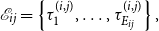 \begin{equation} \mathcal{E}_{ij} = \left\{\tau _1^{(i,j)}, \ldots, \tau _{E_{ij}}^{(i,j)}\right\}, \end{equation}
where $E_{ij}$
is the total number of times
$E_{ij}$
is the total number of times $i$
interacts with
$i$
interacts with $j$
before
$j$
before $T$
or, equivalently, the number of edges connecting
$T$
or, equivalently, the number of edges connecting $i$
with
$i$
with $j$
. Also,
$j$
. Also, $E = \sum _{i,j} E_{ij}$
. We assume that the interaction times in the above equation are the realization of an inhomogeneous Poisson point process with instantaneous rate function denoted with
$E = \sum _{i,j} E_{ij}$
. We assume that the interaction times in the above equation are the realization of an inhomogeneous Poisson point process with instantaneous rate function denoted with $\lambda _{ij}(t) \geq 0,\ \forall t \in [0,T]$
and nodes
$\lambda _{ij}(t) \geq 0,\ \forall t \in [0,T]$
and nodes $i$
and
$i$
and $j$
. Using a more convenient (but equivalent) characterization, we state that the waiting time for a new interaction event between
$j$
. Using a more convenient (but equivalent) characterization, we state that the waiting time for a new interaction event between $i$
and
$i$
and $j$
is exponential with a variable rate that changes over time. Then, if we assume that the inhomogeneous point processes are independent for all pairs
$j$
is exponential with a variable rate that changes over time. Then, if we assume that the inhomogeneous point processes are independent for all pairs $i$
and
$i$
and $j$
, the likelihood function for the rates can be written as:
$j$
, the likelihood function for the rates can be written as:
 \begin{equation} \mathcal{L}\!\left (\boldsymbol{\lambda }\right ) = \prod _{i,j:\ i < j} \left [\left (\prod _{\tau _e \in \mathcal{E}_{ij}} \lambda _{ij}(\tau _e)\right ) \exp \left \{-\int _{0}^{T} \lambda _{ij}(t)dt\right \}\right ], \end{equation}
where, for simplicity, we have removed the superscript $(i,j)$
from
$(i,j)$
from $\tau _e^{(i,j)}$
. In the sections below, we will specify the conditions that make the processes independent across all node pairs.
$\tau _e^{(i,j)}$
. In the sections below, we will specify the conditions that make the processes independent across all node pairs.
2.2 Latent positions
Our goal is to embed the nodes of the network into a latent space, such that the latent positions are the primary driving factor behind the frequency and timing of the interactions between the nodes. Crucially, since the time dimension is continuous and interactions can happen at any point in time, we aim at creating a modeling framework which also evolves continuously over time. Thus, the fundamental assumption of our model is that, at any point in time, the Poisson rate function $\lambda _{ij}(t)$
is determined by the latent positions of the corresponding nodes, which we denote
$\lambda _{ij}(t)$
is determined by the latent positions of the corresponding nodes, which we denote $\textbf{z}_i(t) \in \mathbb{R}^2$
and
$\textbf{z}_i(t) \in \mathbb{R}^2$
and $\textbf{z}_j(t) \in \mathbb{R}^2$
.
$\textbf{z}_j(t) \in \mathbb{R}^2$
.
Remark. We assume that the number of dimensions of the latent space is equal to $2$
, because the main interest of the proposed approach is in latent space visualization of the network. However, we note that the generative model presented in this section can be easily extended to the case
$2$
, because the main interest of the proposed approach is in latent space visualization of the network. However, we note that the generative model presented in this section can be easily extended to the case $\textbf{z}_i(t) \in \mathbb{R}^d$
, with
$\textbf{z}_i(t) \in \mathbb{R}^d$
, with $d>2$
.
$d>2$
.
To facilitate the inference task, the trajectories are assumed to be piece-wise linear curves, characterized by a number of user-defined change points in the time dimension. These change points are in common across the trajectories of all nodes, and they determine the points in time when the linear motions of the nodes change direction and speed. This means that we must define a grid of the time dimension through $K$
change points
$K$
change points
 \begin{equation*} 0=\eta _1 < \eta _2 < \ldots < \eta _{K-1} < \eta _K = T \end{equation*}
that are common across all trajectories. We stress that this modeling choice is only meant to restrict the variety of continuous trajectories that we may consider, as it allows us to use a tractable parametric structure while keeping a high flexibility regarding the trajectories, as the number of change points increases. Also, we make the assumption that, within any two consecutive critical points, the speed at which any given node moves remains constant. As a consequence, we only need to store the coordinates of the nodes at the change points, since all the intermediate positions can then be obtained with:
 \begin{equation} \textbf{z}_i\left ((1-t)\eta _k + t\eta _{k+1}\right ) = (1-t)\textbf{z}_i\left (\eta _k\right ) + t\textbf{z}_i\left (\eta _{k+1}\right ) \quad \quad \forall t \in [0,1] \end{equation}
for any change points $\eta _k$
and
$\eta _k$
and $\eta _{k+1}$
and node
$\eta _{k+1}$
and node $i$
. Under this parametrization of the trajectories, we can increase the number of change points to allow for more flexible structures, at the expense of computational efficiency since this would also increase the number of model parameters to estimate. The choice of the number of change points is made by the user, who defines directly the level of refinement of the trajectories based on the available computing resources.
$i$
. Under this parametrization of the trajectories, we can increase the number of change points to allow for more flexible structures, at the expense of computational efficiency since this would also increase the number of model parameters to estimate. The choice of the number of change points is made by the user, who defines directly the level of refinement of the trajectories based on the available computing resources.
2.2.1 Projection model
Similarly to the foundational paper of Hoff et al. (Reference Hoff, Raftery and Handcock2002), we introduce two possible characterizations of the rates through the latent positions: one is inspired by the projection model and the other is inspired by the distance model. In our projection model, we assume that the rate of interactions is specified by:
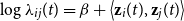 \begin{equation*} \log \lambda _{ij}(t) = \beta + \left \langle \textbf {z}_i(t), \textbf {z}_j(t) \right \rangle \end{equation*}
for all $t \in [0,T]$
and for all nodes
$t \in [0,T]$
and for all nodes $i$
and
$i$
and $j$
. Here,
$j$
. Here, $\beta \in \mathbb{R}$
is an intercept parameter regulating the overall interaction rates in a homogeneous fashion, but extensions of the model where it becomes specific to each node can also be considered. As regards the contributions of the latent positions, the further the nodes are positioned from the origin, the more frequent their interactions will be, especially toward other nodes that are aligned in the same direction.Footnote
1
Vice versa, we are not expecting frequent interactions for nodes that are located too close to the origin, or between pairs of nodes forming an obtuse angle.
$\beta \in \mathbb{R}$
is an intercept parameter regulating the overall interaction rates in a homogeneous fashion, but extensions of the model where it becomes specific to each node can also be considered. As regards the contributions of the latent positions, the further the nodes are positioned from the origin, the more frequent their interactions will be, especially toward other nodes that are aligned in the same direction.Footnote
1
Vice versa, we are not expecting frequent interactions for nodes that are located too close to the origin, or between pairs of nodes forming an obtuse angle.
By taking the logarithm of Equation (2) and replacing $\lambda _{ij}(t)$
, the log-likelihood for the projection model is:
$\lambda _{ij}(t)$
, the log-likelihood for the projection model is:
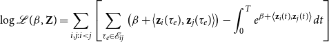 \begin{equation} \log \mathcal{L}(\beta, \textbf{Z}) = \sum _{i,j: i < j}\left [\sum _{\tau _e \in \mathcal{E}_{ij}} \left ( \beta + \left \langle \textbf{z}_i(\tau _e), \textbf{z}_j(\tau _e) \right \rangle \right ) - \int _{0}^T e^{\beta + \left \langle \textbf{z}_i(t), \textbf{z}_j(t) \right \rangle }dt \right ] \end{equation}
As we discuss in Appendix A, the integral term appearing in Equation (4) does not generally have a straightforward analytical solution. So, we take advantage of the fact that the integrand function is fairly regular, to efficiently estimate the integral with a composite Simpson’s rule (see equation 5.1.16 of Atkinson, Reference Atkinson1991).
2.2.2 Distance model
Here, we introduce a version of the LPM that uses the latent Euclidean distances between the nodes, rather than the dot products. The distance model formulation provides easier interpretability than the projection model, and, as we show in the simulation studies (Section 5), it also provides great flexibility, hence generally leading to superior results in this context where the hidden space is in low dimension (two).
In the distance model, we assume that:
 \begin{equation} \log \lambda _{ij}(t) = \beta - \|\textbf{z}_i(t) - \textbf{z}_j(t)\|^2 \end{equation}
where the last term corresponds to the squared Euclidean distance between nodes $i$
and
$i$
and $j$
at time
$j$
at time $t$
. The interpretation of
$t$
. The interpretation of $\beta \in \mathbb{R}$
is analogous to the projection model. By taking the logarithm of Equation (2) and using Equation (5), the log-likelihood of the distance model becomes:
$\beta \in \mathbb{R}$
is analogous to the projection model. By taking the logarithm of Equation (2) and using Equation (5), the log-likelihood of the distance model becomes:
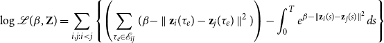 \begin{equation} \log \mathcal{L}(\beta,\textbf{Z}) = \sum _{i,j: i < j} \left \{ \left (\sum _{\tau _e \in \mathcal{E}_{ij}} (\beta - \parallel \textbf{z}_{i}(\tau _e) - \textbf{z}_{j}(\tau _e) \parallel ^2) \right ) - \int _{0}^T e^{\beta - \parallel \textbf{z}_{i}(s) - \textbf{z}_{j}(s) \parallel ^2} ds \right \} \end{equation}
Unlike the projection model, the above log-likelihood has a closed form, since the integral inside the brackets can be calculated analytically (proof in Appendix B).
2.3 Penalized likelihood
Due to the piece-wise linearity assumption in Equation (5), for each node we only need to estimate its positions at times $\{\eta _k\}_{k \in [K]}$
. In order to avoid over fitting, and to obtain more interpretable and meaningful results, we introduce likelihood penalizations based on the latent positions parameters at
$\{\eta _k\}_{k \in [K]}$
. In order to avoid over fitting, and to obtain more interpretable and meaningful results, we introduce likelihood penalizations based on the latent positions parameters at $\{\eta _k\}_{k \in [K]}$
. In particular, a penalization term is included on the right-hand size of Equation (6), whose effect is to disfavor large velocities of the nodes in the latent space.
$\{\eta _k\}_{k \in [K]}$
. In particular, a penalization term is included on the right-hand size of Equation (6), whose effect is to disfavor large velocities of the nodes in the latent space.
For both the projection and distance model, as likelihood penalizations,Footnote 2 we define Gaussian random walk priors on the critical points of the latent trajectories:
 \begin{equation} \begin{split} &\textbf{z}_i(\eta _{k+1})\ |\ \textbf{z}_i(\eta _k)\stackrel{\perp }{\sim } \mathcal{N}\left (\textbf{z}_i(\eta _k), (\eta _{k+1}-\eta _{k})\sigma ^2I_2 \right )\quad \quad \forall k=1,\ldots,K-1 \end{split} \end{equation}
for every node $i$
where
$i$
where $I_2$
is the identity matrix of order two. The equation above (with
$I_2$
is the identity matrix of order two. The equation above (with $\sigma ^2=1$
) would correspond to a Brownian motion for the
$\sigma ^2=1$
) would correspond to a Brownian motion for the $i$
th latent trajectory, except that we would only observe it at the change points, where the latent positions are estimated. However, as the number of change points increases, the prior that we specify tends to a scaled Brownian motion on the plane. The parameter
$i$
th latent trajectory, except that we would only observe it at the change points, where the latent positions are estimated. However, as the number of change points increases, the prior that we specify tends to a scaled Brownian motion on the plane. The parameter $\sigma ^2$
is user-defined; hence, it can be reduced to penalize the movements of the nodes between consecutive change points. In order to obtain sensible penalizations, we choose small values of the variance parameters, as to ensure that the speed of the nodes along the trajectories is not too large. In this way, the nodes are forced to move as little as necessary, making the latent visualization of the network easier to read and interpret, and ensuring that the latent space only captures the critical features that are present in the data.
$\sigma ^2$
is user-defined; hence, it can be reduced to penalize the movements of the nodes between consecutive change points. In order to obtain sensible penalizations, we choose small values of the variance parameters, as to ensure that the speed of the nodes along the trajectories is not too large. In this way, the nodes are forced to move as little as necessary, making the latent visualization of the network easier to read and interpret, and ensuring that the latent space only captures the critical features that are present in the data.
Remark. The likelihood function of the original latent distance model of Hoff et al. (Reference Hoff, Raftery and Handcock2002) is not identifiable with respect to translations, rotations, and reflections of the latent positions. This is a challenging issue in a Bayesian setting that relies on sampling from the posterior distribution. In fact, the posterior samples become non-interpretable, since rigid transformations may have occurred during the collection of the sample (Shortreed et al., Reference Shortreed, Handcock and Hoff2006). These non-identifiabilities are not especially relevant in our optimization setting, since the equivalent configurations of model parameters lead to the same qualitative results and interpretations. However, a case for non-identifiability can be made for dynamic networks, since translations, rotations, and reflections can occur across time, thus affecting results and interpretation. The penalizations that we introduce in this paper ensure that the nodes move as little as necessary, thus disfavoring any rotations, translations, and reflections of the space. As a consequence, the penalizations directly address the identifiability issues and the latent point process remains comparable across time.
3. Inference
In this section, we discuss the inference for the distance model described in Section 2.2.2, but an analogous procedure is considered for the projection model.
Recalling that we work with undirected graphs and in force of Equation (7), the penalized log-likelihood is
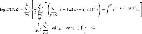 \begin{equation} \begin{split} \log \mathcal{L}(\beta, \textbf{Z}) &= \sum _{i=1}^{N} \left \{ \frac{1}{2}\sum _{\substack{j=1 \\ j\neq i}}^N \left [\left (\sum _{\tau _e \in \mathcal{E}_{ij}} (\beta - \parallel \textbf{z}_{i}(\tau _e) - \textbf{z}_{j}(\tau _e) \parallel ^2) \right ) - \int _{0}^T e^{\beta - \parallel \textbf{z}_{i}(s) - \textbf{z}_{j}(s) \parallel ^2} ds\right ] \right .\\ &\hspace{1cm}\left . - \frac{1}{2\sigma ^2} \sum _{k=1}^K \parallel \textbf{z}_i(\eta _{k}) - \textbf{z}_i(\eta _{k-1}) \parallel ^2 \right \} + C, \\ \end{split} \end{equation}
where $C$
is a constant term that does not depend on (
$C$
is a constant term that does not depend on ( $\beta$
,
$\beta$
, $\textbf{Z}$
) and the integral can be explicitly computed as shown in Appendix B. Since the log-likelihood has a closed form, we implement it and rely on automatic differentiation (Griewank, Reference Griewank1989; Baydin et al., Reference Baydin, Pearlmutter, Radul and Siskind2018) to maximize it numerically, with respect to
$\textbf{Z}$
) and the integral can be explicitly computed as shown in Appendix B. Since the log-likelihood has a closed form, we implement it and rely on automatic differentiation (Griewank, Reference Griewank1989; Baydin et al., Reference Baydin, Pearlmutter, Radul and Siskind2018) to maximize it numerically, with respect to $(\beta, \textbf{Z})$
, via gradient descent (GD).Footnote
3
Note that, as pointed out in the previous section, maximizing the above-penalized log-likelihood is equivalent to performing maximum-a-posteriori inference. Moreover, as it can be seen in Equation (8), the log-likelihood is additive in the number of nodes. This remark allows us to speed up the inference of the model parameters by means of SGD (Bottou, Reference Bottou2010). Indeed, let us introduce
$(\beta, \textbf{Z})$
, via gradient descent (GD).Footnote
3
Note that, as pointed out in the previous section, maximizing the above-penalized log-likelihood is equivalent to performing maximum-a-posteriori inference. Moreover, as it can be seen in Equation (8), the log-likelihood is additive in the number of nodes. This remark allows us to speed up the inference of the model parameters by means of SGD (Bottou, Reference Bottou2010). Indeed, let us introduce $\psi _1, \ldots, \psi _n$
such that
$\psi _1, \ldots, \psi _n$
such that
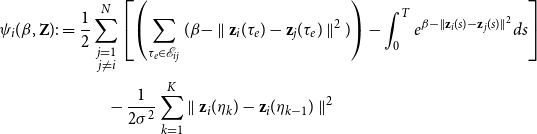 \begin{equation} \begin{split} \psi _i(\beta, \textbf{Z}) :&= \frac{1}{2}\sum _{\substack{j = 1 \\ j \neq i}}^N \left [\left (\sum _{\tau _e \in \mathcal{E}_{ij}}(\beta - \parallel \textbf{z}_{i}(\tau _e) - \textbf{z}_{j}(\tau _e) \parallel ^2) \right ) - \int _{0}^T e^{\beta - \parallel \textbf{z}_{i}(s) - \textbf{z}_{j}(s) \parallel ^2} ds\right ] \\ &\hspace{1cm}- \frac{1}{2\sigma ^2} \sum _{k=1}^K \parallel \textbf{z}_i(\eta _{k}) - \textbf{z}_i(\eta _{k-1}) \parallel ^2 \end{split} \end{equation}
and a discrete random variable $\Psi (\beta, \textbf{Z})$
such that
$\Psi (\beta, \textbf{Z})$
such that
 \begin{equation*} \pi \,:\!=\, \pi _i \,:\!=\, \mathbb {P}\{\Psi (\beta, \textbf {Z})=\psi _i(\beta, \textbf {Z})| \textbf {Z}\} = \frac {1}{N}, \qquad \forall i \in \{1,\ldots, N\} \end{equation*}
where we stress that the above probability is conditional to $\textbf{Z}$
and given the model parameter
$\textbf{Z}$
and given the model parameter $\beta$
. Then, let us denote
$\beta$
. Then, let us denote $\nabla$
the gradient operator with respect to
$\nabla$
the gradient operator with respect to $(\beta, \textbf{Z})$
and
$(\beta, \textbf{Z})$
and $\mathbb{E}_{\pi }$
the expectation taken with respect to the probability measure
$\mathbb{E}_{\pi }$
the expectation taken with respect to the probability measure $\pi$
introduced above (and hence with
$\pi$
introduced above (and hence with $\textbf{Z}$
given). Then, we have the following
$\textbf{Z}$
given). Then, we have the following
Proposition 1. $N\nabla \Psi{(\beta,\textbf{Z})}$
is an unbiased estimator of
$N\nabla \Psi{(\beta,\textbf{Z})}$
is an unbiased estimator of $\nabla \log \mathcal{L}(\beta, \textbf{Z})$
.
$\nabla \log \mathcal{L}(\beta, \textbf{Z})$
.
Proof.
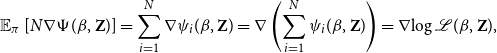 \begin{equation*} \mathbb {E}_{\pi }\left [ N\nabla \Psi (\beta,\textbf {Z}) \right ] = \sum _{i=1}^N \nabla \psi _i{(\beta,\textbf {Z})} = \nabla \left ({\sum _{i=1}^N \psi _i}(\beta,\textbf {Z})\right ) = \nabla {\log \mathcal {L}(\beta,\textbf {Z})}, \end{equation*}
where the last equality follows from the additivity of the gradient operator.
The above proposition allows us to sample (subsets of) nodes uniformly at random, with re-injection, and use each sample (a.k.a. mini-batch) to update the model parameters via SGD, as shown in Bottou (Reference Bottou2010). In more details, if $\theta \,:\!=\, \{\beta, \boldsymbol{Z}\}$
denotes the set of the model parameters, at the
$\theta \,:\!=\, \{\beta, \boldsymbol{Z}\}$
denotes the set of the model parameters, at the $k$
th iteration of the SGD algorithm,
$k$
th iteration of the SGD algorithm, $\theta$
is updated as follows
$\theta$
is updated as follows
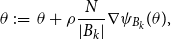 \begin{equation*} \theta \,:\!=\, \theta + \rho \frac {N}{|B_k|}\nabla \psi _{B_k}(\theta ), \end{equation*}
where the hyper-parameter $\rho$
is the learning rate,
$\rho$
is the learning rate, $B_k$
is a set of
$B_k$
is a set of $|B_k|$
nodes extracted uniformly at random and
$|B_k|$
nodes extracted uniformly at random and $\psi _{B_k}(\theta )$
refers to the estimator of the full-batch log-likelihood, based on the data batch
$\psi _{B_k}(\theta )$
refers to the estimator of the full-batch log-likelihood, based on the data batch $B_k$
, namely:
$B_k$
, namely:
 \begin{align*} \begin{split} \psi _{B_k}(\beta, \textbf{Z}) :&= \frac{1}{2}\sum _{i \in B_k}\left [\sum _{\substack{j = 1 \\ j \neq i}}^N \left (\sum _{\tau _e \in \mathcal{E}_{ij}}(\beta - \parallel \textbf{z}_{i}(\tau _e) - \textbf{z}_{j}(\tau _e) \parallel ^2) \right ) - \int _{0}^T e^{\beta - \parallel \textbf{z}_{i}(s) - \textbf{z}_{j}(s) \parallel ^2} ds\right ] \\ &- \frac{1}{2\sigma ^2} \sum _{k=1}^K \parallel \textbf{z}_i(\eta _{k}) - \textbf{z}_i(\eta _{k-1}) \parallel ^2. \end{split} \end{align*}
We stress that, if $|B_k| = 1$
, the above equation reduces to Equation (9); conversely if
$|B_k| = 1$
, the above equation reduces to Equation (9); conversely if $|B_k| = N$
SGD reduces to full-batch GD. We finally note that the above two equations state that the model parameters can be updated, at each iteration, based on a sub-graph with
$|B_k| = N$
SGD reduces to full-batch GD. We finally note that the above two equations state that the model parameters can be updated, at each iteration, based on a sub-graph with $N$
nodes whose links are uniquely those connecting the nodes in
$N$
nodes whose links are uniquely those connecting the nodes in $B_k$
with their neighbors of order one (a.k.a. friends). We have implemented the estimation algorithm and visualization tools in a software repository, called CLPM, which is publicly available (CLPM GitHub repository, 2021).
$B_k$
with their neighbors of order one (a.k.a. friends). We have implemented the estimation algorithm and visualization tools in a software repository, called CLPM, which is publicly available (CLPM GitHub repository, 2021).
4. Interpretation and model-based summaries
Both the distance and the projection model provide a visual representation of the latent space as output. Due to the continuous time dimension, the results are most easily shown as a video. For this paper, the code and results (including videos) are publicly available from CLPM GitHub repository (2021).
The evolution of the latent space provides a visualization which can be used to qualitative assess the connectivity, both at the global level (e.g., contractions and expansions of the latent space) as well as at a local level (e.g., which nodes have more connections and when).
For the projection model, we expect highly connected nodes to be located far from the origin. They would have a higher chance to interact with any other node. On the other hand, nodes that are close to the origin will have lower connectivity, overall. For both types of nodes, the angle in between them will also play a role, favoring interactions between nodes that point in the same direction. For the distance model, we are expecting nodes to take more central positions as they become more active, and, clearly, communities arise when clusters of points are observed.
Clusteredness
In order to capture this particular behavior, we introduce a quantitative measure of clustering, or “clusteredness” of the latent space. The goal of this index is to capture and measure the local contractions of the latent space, whereby nodes tend to aggregate into clusters at a particular point in time. To construct this measure, we choose an arbitrary threshold value $\varphi$
and consider circles of radius
$\varphi$
and consider circles of radius $\varphi$
around each of the nodes, in the latent space. If we consider an arbitrary node, we want to count how many other nodes fall within its circle, at each point in time. By averaging this measure across all nodes, we obtain our clusteredness index, defined as the average number of nodes that fall within a random node’s circle.
$\varphi$
around each of the nodes, in the latent space. If we consider an arbitrary node, we want to count how many other nodes fall within its circle, at each point in time. By averaging this measure across all nodes, we obtain our clusteredness index, defined as the average number of nodes that fall within a random node’s circle.
This measure evolves continuously over time, and we can easily calculate it from the algorithm’s output. The relative increases and decreases of the measure over time can permit an appreciation of how the latent space can locally contract, to create communities within the network.
Partition
An additional model-based summary that we consider is a partitioning of the nodes of the network. Based on the latent space representation, we aim at deriving a partitioning of the nodes, whereby nodes in the same group tend to spend more time close to each other. This is achieved by calculating a similarity value for each pair of nodes $(i,j)$
, at each change point
$(i,j)$
, at each change point $\eta$
, equal to
$\eta$
, equal to $\exp \{-\parallel \textbf{z}_{i}(\eta ) - \textbf{z}_{j}(\eta ) \parallel ^2\}$
. Then, we can aggregate the pairwise similarities over time by calculating their median and use these node similarities as an input for a spectral clustering algorithm (the number of groups for the algorithm is user-defined).
$\exp \{-\parallel \textbf{z}_{i}(\eta ) - \textbf{z}_{j}(\eta ) \parallel ^2\}$
. Then, we can aggregate the pairwise similarities over time by calculating their median and use these node similarities as an input for a spectral clustering algorithm (the number of groups for the algorithm is user-defined).
This approach provides additional information (in the videos and plots, these clusters can be indicated with the different nodes’ colors), and it provides a higher-level visualization and summarization of the model’s results. We note that, ideally, a challenging but interesting idea would be to include these clustering aspects directly into the generative process of the model; however, we do not pursue this here and leave the extension as future work.
Goodness of fit
We consider a basic measure of model fit whereby we calculate the observed number of interactions:
 \begin{equation*} u_{ijk} = \sum _{\tau _{e} \in \mathcal {E}_{ij}} {\unicode {x1D7D9}}_{\{\eta _k \leq \tau _e < \eta _{k+1} \}} \end{equation*}
Here, ${\unicode{x1D7D9}}_{\{\mathcal{A}\}}$
is equal to one if the event
${\unicode{x1D7D9}}_{\{\mathcal{A}\}}$
is equal to one if the event $\mathcal{A}$
is true or zero otherwise. In addition, we calculate the corresponding expectation according to our model:
$\mathcal{A}$
is true or zero otherwise. In addition, we calculate the corresponding expectation according to our model:
 \begin{equation*} \hat {u}_{ijk} = \int _{\eta _k}^{\eta _{k+1}} \lambda _{ij}(t) dt \end{equation*}
Then, we calculate the absolute value difference between the two values and average it across all edge pairs and across all change points. This corresponds to a measure of in-sample prediction error for the number of interactions. We emphasize that choosing this particular measure is arbitrary, and in fact, more sophisticated measures may be constructed (e.g., see Yang et al., Reference Yang, Rao and Neville2017; Huang et al., Reference Huang, Soliman, Paul and Xu2022) to provide a better assessment of the goodness of fit. Our measure can be used to compare different models (i.e., distance model against projection model or different choices of the penalization parameter $\sigma ^2$
or the number of the latent dimensions), as long as the change points in the two models are located identically. On the other hand, the measure is sensitive to the change point choice, in that the average number of interactions per time segment directly affects the magnitude of the mean absolute error.
$\sigma ^2$
or the number of the latent dimensions), as long as the change points in the two models are located identically. On the other hand, the measure is sensitive to the change point choice, in that the average number of interactions per time segment directly affects the magnitude of the mean absolute error.
5. Experiments: Synthetic data
In this section, we illustrate applications of our methodology on artificial data. We propose two types of frameworks: in the first one, we consider dynamic block structures (which involve the presence of communities, hubs, and isolated points). In this case, our aim is to inspect how the network dynamics are captured by CLPM. In the second framework, we generate data using the distance CLPM and we aim at recovering the simulated trajectories for each node.
5.1 Dynamic block structures
Simulation study 1
In this first experiment, we use a data generative mechanism that relies on a dynamic blockmodel structure for instantaneous interactions (Corneli et al., Reference Corneli, Latouche and Rossi2018). We specifically focus on a special case of a dynamic stochastic blockmodel where we can have community structure, but we cannot have disassortative mixing, that is, the rate of interactions within a community cannot be smaller than the rate of interactions between communities. In this framework, the dynamic stochastic blockmodel approximately corresponds to a special case of our distance CLPM, whereby the nodes clustered together essentially are located nearby.
In the generative framework that we consider the only node-specific information is the cluster label, hence, this structure is not as flexible as the CLPM as regards modeling node’s individual behaviors. So, our goal here is to obtain a latent space visualization for these data and to ensure that CLPM can accurately capture and highlight the presence of communities. An aspect of particular importance is how CLPM reacts to the creation and dissolution of communities over time: for this purpose, our generated data include changes in the community structure over time.
For this setup, we consider the time interval $[0,40]$
(for simplicity, we use seconds as a unit measure of time) and divide this into four consecutive time segments of
$[0,40]$
(for simplicity, we use seconds as a unit measure of time) and divide this into four consecutive time segments of $10$
s each. In each of the four time segments,
$10$
s each. In each of the four time segments, $60$
nodes are arranged into different community structures. Thus, any changes in community structure are synchronous for all nodes and they happen at the endpoints of a time segment. The rate of interactions between any two nodes is determined by their group allocations in that specific time segment. The rate remains constant in each time segment, so that we effectively have a piece-wise homogeneous Poisson process over time, for each dyad.
$60$
nodes are arranged into different community structures. Thus, any changes in community structure are synchronous for all nodes and they happen at the endpoints of a time segment. The rate of interactions between any two nodes is determined by their group allocations in that specific time segment. The rate remains constant in each time segment, so that we effectively have a piece-wise homogeneous Poisson process over time, for each dyad.
We denote with $X^{(s)} \in \mathbb{N}^{N\times N}$
a simulated weighted interaction matrix which counts how many interactions occur in the
$X^{(s)} \in \mathbb{N}^{N\times N}$
a simulated weighted interaction matrix which counts how many interactions occur in the $s$
th time segment for each dyad:
$s$
th time segment for each dyad:
 \begin{equation*} X^{(s)}_{ij} | \textbf {C} \sim \mathcal {P}\left (\theta _{\textbf {c}_i \textbf {c}_j}^{(s)} \right ), \end{equation*}
where $\mathcal{P}(\cdot )$
indicates the Poisson probability mass function, and
$\mathcal{P}(\cdot )$
indicates the Poisson probability mass function, and $\textbf{C}$
is a latent vector of length
$\textbf{C}$
is a latent vector of length $N$
indicating the cluster labels of each of the nodes. Once we know the number of interactions for each dyad and each segment, the timing of these interactions can be sampled from a uniform distribution in the respective time segment. More in detail, the rate parameters are characterized as follows:
$N$
indicating the cluster labels of each of the nodes. Once we know the number of interactions for each dyad and each segment, the timing of these interactions can be sampled from a uniform distribution in the respective time segment. More in detail, the rate parameters are characterized as follows:
-
(i) in the time segment $[0,10[$
, the expected number of interactions is the same for every pair of nodes:
$\theta ^{(1)}_{\textbf{c}_1 \textbf{c}_j} = 1$
, for all
$i$
and
$j$
;
$[0,10[$
, the expected number of interactions is the same for every pair of nodes:
$\theta ^{(1)}_{\textbf{c}_1 \textbf{c}_j} = 1$
, for all
$i$
and
$j$
; -
(ii) in the time segment
$[10,20[$
, three communities emerge, in particular
$\theta ^{(2)}_{11} = 10$
,
$\theta ^{(2)}_{22} = 5$
and
$\theta ^{(2)}_{33} = 1$
, whereas the rate for any two nodes in different communities is
$1$
; -
(iii) in the time segment
$[20,30[$
, the first community splits and each half joins a different existing community. The two remaining communities are characterized by
$\theta ^{(3)}_{11} = \theta ^{(3)}_{22} = 5$
. Again, any two nodes in different communities interact with rate
$1$
; -
(iv) in the time segment
$[30,40]$
, we are back to the same structure as in (i).


Throughout the simulation, node $1$
always behaves as a hub, and node
$1$
always behaves as a hub, and node $60$
is always isolated. This means that node
$60$
is always isolated. This means that node $1$
interacts with rate
$1$
interacts with rate $10$
at all times with any other node, whereas node
$10$
at all times with any other node, whereas node $60$
interacts with rate
$60$
interacts with rate $0.01$
at all times with any other node, regardless of any cluster label.
$0.01$
at all times with any other node, regardless of any cluster label.
In Figure 1, we show a collection of snapshots at some critical time points, for the projection model.
Simulation study 1: snapshots for the projection model. The sizes and colors (fading from blue to yellow) of the nodes reflect their current level of interaction. The hub and the isolated node are colored in green and red, respectively.

The full videos of the results are provided in the code repository. The main observation is that the communities are clearly captured at all times, and they are clearly visually separated. In the two cluster formation, we see that the clusters are almost aligned to the axes; hence, they point in perpendicular directions. In the three cluster formation, the non-community third cluster, which has low interaction rate, is instead positioned more centrally between the two, but still separated from the others. This is perhaps surprising since this group should is expected to have fewer interactions and a weaker community structure. The hub is always located very far from the origin and from other points, since this guarantees a large dot product value with respect to all other nodes, at all times. By contrast, the isolated node is always located toward the opposite direction, which is very reasonable.
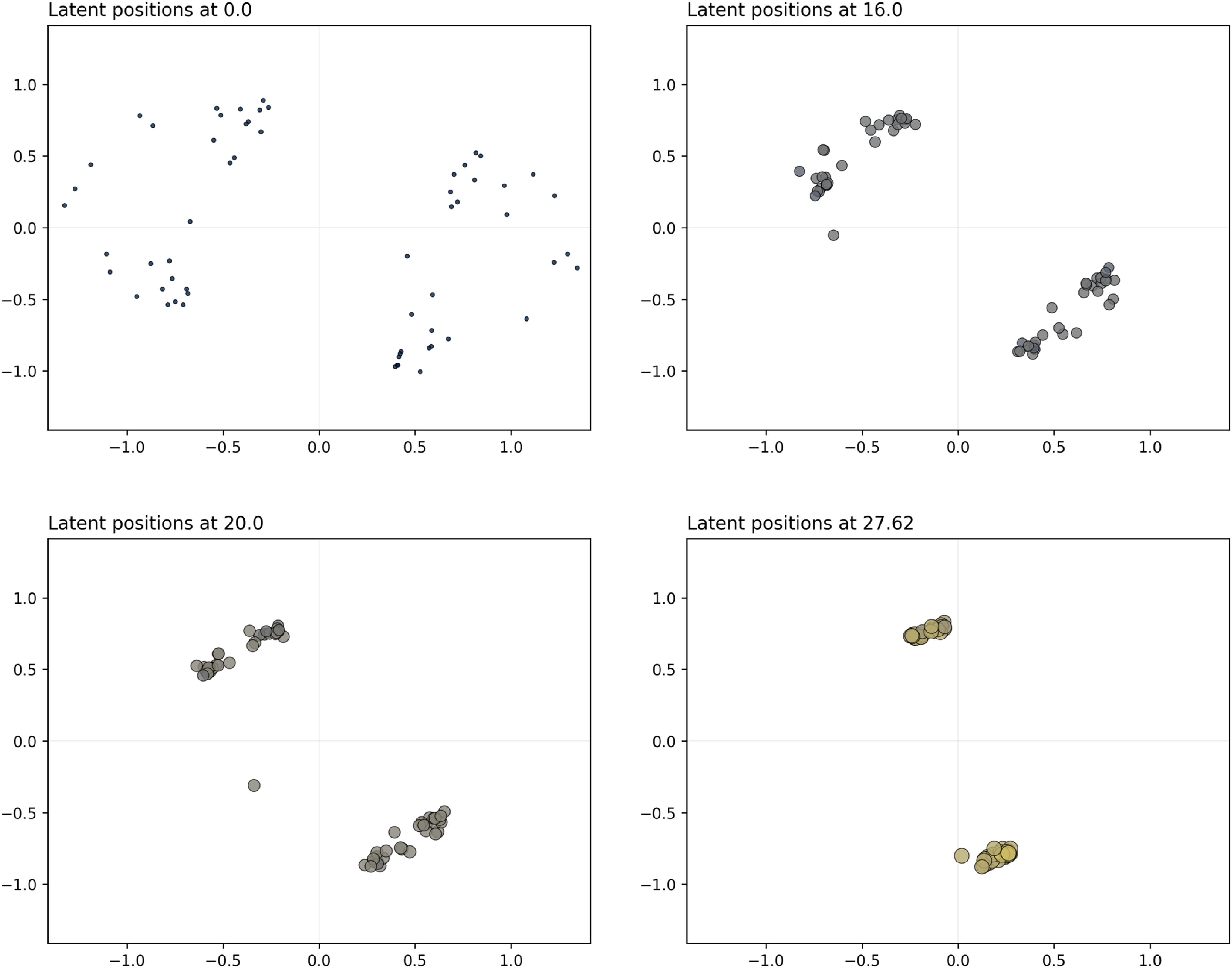
Figure 2 shows instead the snapshots for the distance model. In this case, the clusters are clearly separated at all times. The cluster with a strong community structure is less dispersed than the clusters with a weaker community structure. The hub is constantly positioned in the center of the space, as to minimize the distance from all of the nodes at the same time. The isolated node is instead wandering in the outskirts of the latent social space. The creation and dissolution of communities only happens right at the proximity of start/end of each time segment. For this simulation study, the mean absolute error arising from the goodness of fit procedure is $0.63$
for the projection model against
$0.63$
for the projection model against $0.73$
for the distance model, thus preferring the projection model.
$0.73$
for the distance model, thus preferring the projection model.
Simulation study 1: snapshots for the distance model. The sizes and colors (fading from blue to yellow) of the nodes reflect their current level of interaction. The hub and the isolated node are colored in green and red, respectively.

Technical details regarding the simulation’s parameters, including penalization terms and number of change points, can be consulted on the CLPM code repository.
Simulation study 2
In the second simulation study, we use again a blockmodel structure; however, in this case we approximate a continuous time framework by defining very short time segments and letting the communities change from one time segment to the next. Since creations and dissolutions of communities would be unlikely in such a short period of time, we keep the community memberships unchanged, and we progressively increase the cohesiveness of the communities. This means that we progressively increase the rates of interactions between any pairs of nodes that belong to the same community, while keeping any other rate constant. The rate of interactions within each community starts at value $1$
and increases in a step-wise fashion over
$1$
and increases in a step-wise fashion over $40$
segments, up to the value
$40$
segments, up to the value $5$
. The time interval is
$5$
. The time interval is $[0,40]$
, and we consider two communities. Halfway through the simulation, a special node moves from one community to the other.
$[0,40]$
, and we consider two communities. Halfway through the simulation, a special node moves from one community to the other.
For the projection CLPM, we show the results in Figure 3, whereas Figure 4 shows the results for the distance model. Both approaches clearly capture the reinforcement of the communities over time by aggregating the nodes of each group. We observe this behavior both for the projection model and for the distance model. The projection model also exhibits nodes getting farther from the center of the space, since this would give them higher interaction rates, overall. As concerns the special node moving from one community to the other, this is well captured in that the node transitions smoothly after approximately $20$
s, in both models. As concerns model fit and model choice, the mean absolute error is
$20$
s, in both models. As concerns model fit and model choice, the mean absolute error is $5.48$
for the projection model against
$5.48$
for the projection model against $3.97$
for the distance model, thus preferring the distance model.
$3.97$
for the distance model, thus preferring the distance model.
Simulation study 2: snapshots for the projection model. The sizes and colors (fading from blue to yellow) of the nodes reflect their current level of interaction.
Simulation study 2: snapshots for the distance model. The sizes and colors (fading from blue to yellow) of the nodes reflect their current level of interaction.
5.2 Comparison with the static LPM
For simulation study $2$
, we propose a comparison of our results with a static LPM, as per Hoff et al. (Reference Hoff, Raftery and Handcock2002). We use an implementation of the static LPM available from the R package latentnet.
$2$
, we propose a comparison of our results with a static LPM, as per Hoff et al. (Reference Hoff, Raftery and Handcock2002). We use an implementation of the static LPM available from the R package latentnet.
In order to make the results comparable, we divide the time interval of $40$
s into
$40$
s into $80$
sub-intervals of
$80$
sub-intervals of $0.5$
s each. Then, within each sub-interval, we aggregate the interaction data by creating an edge between all those nodes that have at least one interaction. By doing so, we obtain a sequence of
$0.5$
s each. Then, within each sub-interval, we aggregate the interaction data by creating an edge between all those nodes that have at least one interaction. By doing so, we obtain a sequence of $80$
binary undirected networks, on which we fit the distance model of Hoff et al. (Reference Hoff, Raftery and Handcock2002).
$80$
binary undirected networks, on which we fit the distance model of Hoff et al. (Reference Hoff, Raftery and Handcock2002).
We propose the visual results for four sub-intervals in Figure 5. From these results, we make the following observations:
-
The static LPM does not capture the transition of the special node from one community to the other.
-
The static LPM does not provide a model-based framework to make the snapshots comparable across time frames, due to rotations, translations, and reflections.
-
The static LPM does not provide an initial strong separation of the communities, due to the adaption that is made in discretizing the data over time.
Simulation study 2: fitted static LPM on four sub-intervals. Colors indicate the cluster membership, with one node in red being the transient node that changes community.

On the other hand, the CLPM can address these issues directly by providing a continuous time evolution and thus a more accurate representation of the trajectories, without using any ad hoc data transformation.
5.3 Distance model
Simulation study 3
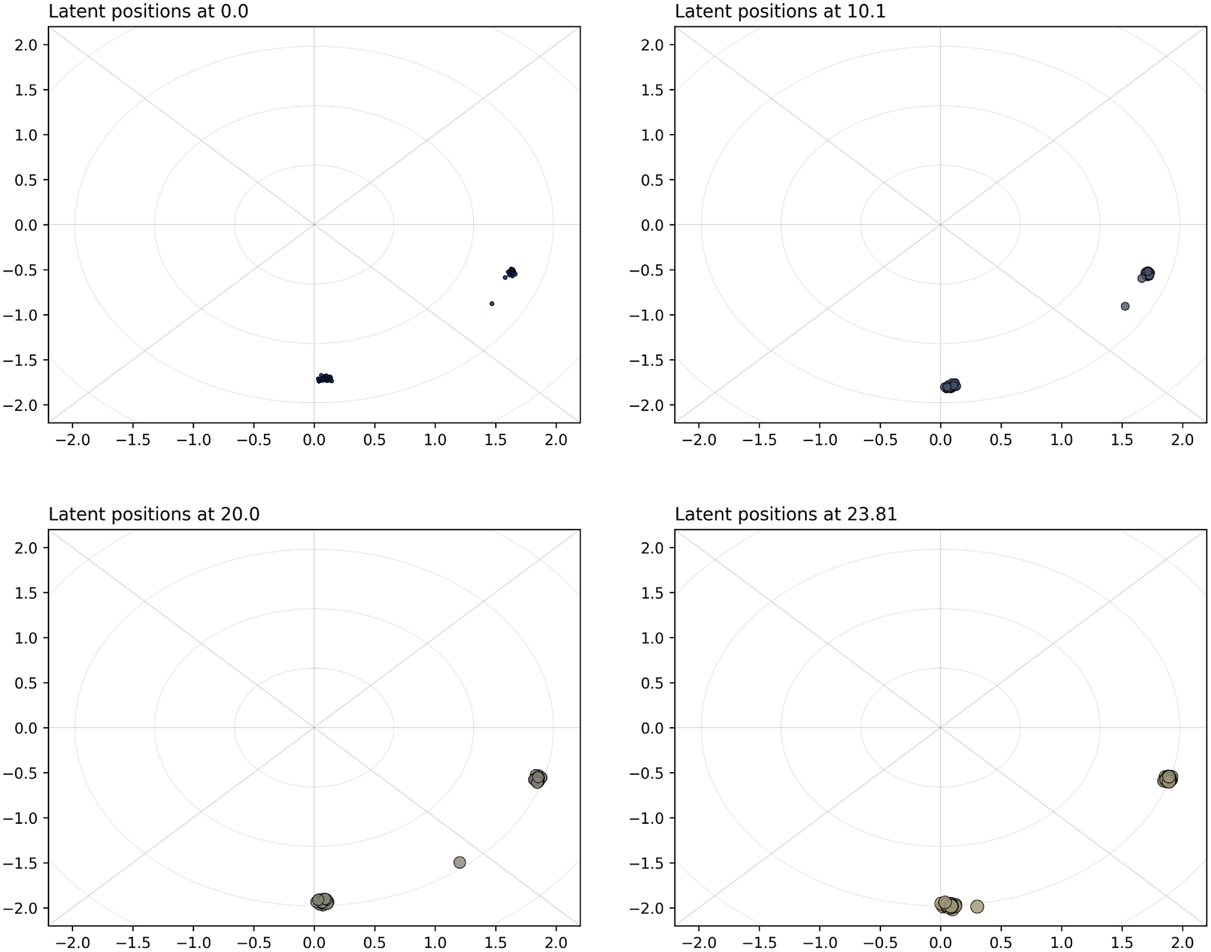
In this simulation study, we generate data from the latent distance model itself (Section 2.2.2). In this case, our goal can be more ambitious, and thus, we aim at reconstructing the individual trajectory of each of the nodes, at every point in time, as accurately as possible. To make the reading of the results easier, we assume that the nodes move along some pre-determined trajectories that are easy to visualize. The $N=20$
nodes start on a ring which is centered at the origin of the space and has radius equal to
$N=20$
nodes start on a ring which is centered at the origin of the space and has radius equal to $1$
. The nodes are located consecutively and in line along the ring, with equal space in between any two consecutive nodes. Then, they start to move at constant speed toward the center of the space, which they reach after
$1$
. The nodes are located consecutively and in line along the ring, with equal space in between any two consecutive nodes. Then, they start to move at constant speed toward the center of the space, which they reach after $5$
s. After reaching the center, they perform the same motion backward, and they are back at their initial positions after
$5$
s. After reaching the center, they perform the same motion backward, and they are back at their initial positions after $5$
more seconds. The trajectories of the nodes make it so that, when the nodes are along the largest ring, their rate of interaction is essentially zero; however, the rate increases as they are closer and closer to the center of the space.
$5$
more seconds. The trajectories of the nodes make it so that, when the nodes are along the largest ring, their rate of interaction is essentially zero; however, the rate increases as they are closer and closer to the center of the space.
Figure 6 shows a collection of snapshots for the projection model. The nodes are approximately equally spaced along a line, and they progress outwards from the center of the space. As they get far apart from the center and from each other, their dot products increase and so do their interaction rates. The projection model, which is not the same model that has generated the data, tends to spread out the nodes on the space, which is ideal and expected from these data. However, this means that some of the nodes almost point in perpendicular directions, which is at odds with the fact that, halfway through the study, all nodes should interact with all others.
Simulation study 3: snapshots for the projection model. The sizes and colors (fading from blue to yellow) of the nodes reflect their current level of interaction.
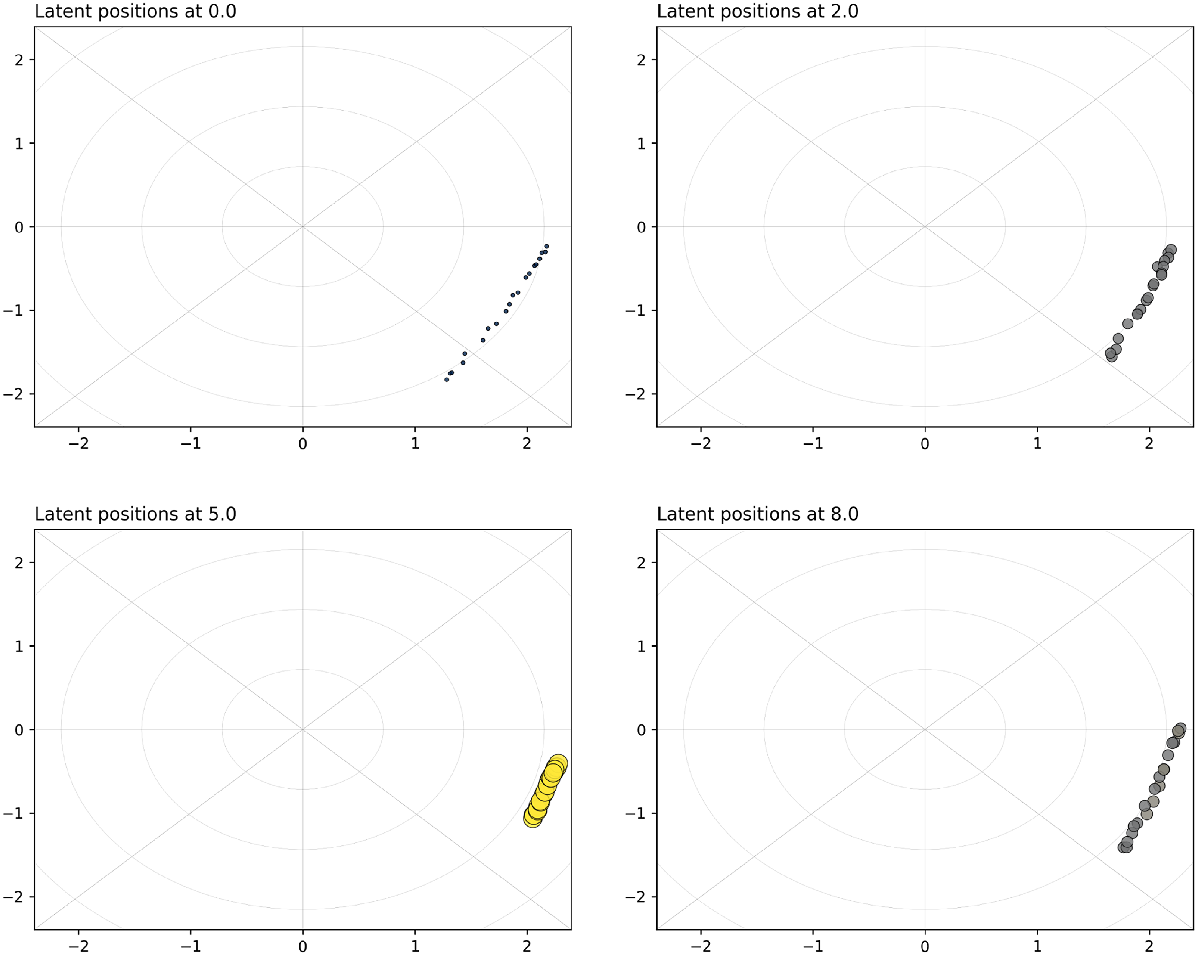
As concerns the results for the distance model, these are shown in Figure 7, and they highlight that the true trajectories are essentially accurately recovered. The model can capture really well the contraction and expansion of the latent space, and the individual trajectories of the nodes are closely following the theoretical counterparts. The scale of the latent space is also correctly estimated since the largest ring has approximately radius $1$
. In addition, the goodness of fit criterion is equal to
$1$
. In addition, the goodness of fit criterion is equal to $43.9$
for the projection model and
$43.9$
for the projection model and $33.6$
for the distance model, thus preferring the distance model. This is an expected result since the data are in fact generated using the distance model itself.
$33.6$
for the distance model, thus preferring the distance model. This is an expected result since the data are in fact generated using the distance model itself.
Simulation study 3: snapshots for the distance model. The sizes and colors (fading from blue to yellow) of the nodes reflect their current level of interaction.

There are some important remarks to make. First, after $5$
s, that is, when all nodes are located close to the center, it is understandable that a rotation or reflection (with respect to the origin of the space) may happen. This is inevitable since the solution can only be recovered up to a rotation/reflection of all the latent trajectories, but also because the first
$5$
s, that is, when all nodes are located close to the center, it is understandable that a rotation or reflection (with respect to the origin of the space) may happen. This is inevitable since the solution can only be recovered up to a rotation/reflection of all the latent trajectories, but also because the first $5$
s and the last
$5$
s and the last $5$
s can technically be seen as two independent problems. The collapse to zero can be seen as a reset in terms of orientation of the latent space. That is because the penalization terms only work with two consecutive change points, so, if we view them as identifiability constraints, they would lose their effectiveness when all the nodes collapse to zero for some time. A second fundamental remark is that the estimation procedure can lead to good results only if we observe an appropriate number of interactions. This is a specific trait of LPMs in general, since we can only guess the position of one node accurately when we know to whom it connects (or, in this context, how frequently), as we would tend to locate it close to its neighbors. In our simulated setting, there are few to no interactions when nodes are along the largest ring, so it makes sense that the results seem a bit more noisy in those instants.
$5$
s can technically be seen as two independent problems. The collapse to zero can be seen as a reset in terms of orientation of the latent space. That is because the penalization terms only work with two consecutive change points, so, if we view them as identifiability constraints, they would lose their effectiveness when all the nodes collapse to zero for some time. A second fundamental remark is that the estimation procedure can lead to good results only if we observe an appropriate number of interactions. This is a specific trait of LPMs in general, since we can only guess the position of one node accurately when we know to whom it connects (or, in this context, how frequently), as we would tend to locate it close to its neighbors. In our simulated setting, there are few to no interactions when nodes are along the largest ring, so it makes sense that the results seem a bit more noisy in those instants.
5.4 Running times
We report some results aiming at quantifying the time gain due to the use of the SGD algorithm detailed in Section 3. We simulated dynamic networks according to the setup of Simulation study 2 (Section 5.1) with number of nodes varying in the range $\{30,60,\ldots,180\}$
. For each number of nodes, the distance model was first fit to the data with (mini) batch size
$\{30,60,\ldots,180\}$
. For each number of nodes, the distance model was first fit to the data with (mini) batch size $N/10$
and 25 epochs.Footnote
4
These settings were checked to be sufficient to numerically reach a stationary point
$N/10$
and 25 epochs.Footnote
4
These settings were checked to be sufficient to numerically reach a stationary point $(\textbf{Z}, \beta )$
stabilizing the log-likelihood. The average log-likelihood (say
$(\textbf{Z}, \beta )$
stabilizing the log-likelihood. The average log-likelihood (say $l$
) on the last epoch was computed and a full-batch GD algorithm was independently run on the same data and stopped either once reaching
$l$
) on the last epoch was computed and a full-batch GD algorithm was independently run on the same data and stopped either once reaching $l$
or after 250 epochs. The same initial (random) values for
$l$
or after 250 epochs. The same initial (random) values for $\textbf{Z}$
and
$\textbf{Z}$
and $\beta$
were adopted for both SGD and GD, with a learning rate of
$\beta$
were adopted for both SGD and GD, with a learning rate of $1.0^{-4}$
for
$1.0^{-4}$
for $\textbf{Z}$
and
$\textbf{Z}$
and $1.0^{-7}$
for
$1.0^{-7}$
for $\beta$
. The running times (seconds) needed to reach
$\beta$
. The running times (seconds) needed to reach $l$
for each number of nodes are reported in Figure 8. As it can be seen, with
$l$
for each number of nodes are reported in Figure 8. As it can be seen, with $N=180$
nodes, the full-batch GD algorithm roughly needs 16 min to converge versus 4 min required by the mini-batch SGD counterpart. The experiment was run on a DELL server PowerEdge T640, equipped with an Intel Xeon processor, 28 cores (12 cores and 27 of RAM memory available on a dedicated virtual machine), and a NVIDIA GeForce RTX 2080 graphic card. The optimization algorithms (GD and SGD) were coded in PyTorch and exploited GPU acceleration.
$N=180$
nodes, the full-batch GD algorithm roughly needs 16 min to converge versus 4 min required by the mini-batch SGD counterpart. The experiment was run on a DELL server PowerEdge T640, equipped with an Intel Xeon processor, 28 cores (12 cores and 27 of RAM memory available on a dedicated virtual machine), and a NVIDIA GeForce RTX 2080 graphic card. The optimization algorithms (GD and SGD) were coded in PyTorch and exploited GPU acceleration.
Time (in seconds) needed to maximize the penalized log-likelihood with full-batch GD (green) and mini-batch SGD (blue).

6. Applications
In this section, we illustrate our approach over three real datasets, highlighting how we can characterize the trajectories of individual nodes, the formation and dissolution of communities, and other types of connectivity patterns. From the simulation studies, we have pointed out that the distance model generally provides a more convenient and appropriate framework to study these aspects of the data. In addition, the distance model is also easier to interpret. So, since our main focus here is on model-based visualization and interpretation, we only show the results for the distance model and redirect the reader to the associated code repository where the complete results can be found also for the projection model.
6.1 ACM hypertext conference dataset
The ACM Hypertext 2009 conference was held over 3 days in Turin, Italy, from June 29 to July 1. At the conference, $113$
attendees wore special badges which recorded an interaction whenever two badges were facing each other at a distance of
$113$
attendees wore special badges which recorded an interaction whenever two badges were facing each other at a distance of $1.5$
m or less, for at least
$1.5$
m or less, for at least $20$
s. For each of these interactions, a timestamp was recorded as well as the identifiers of the two personal badges.
$20$
s. For each of these interactions, a timestamp was recorded as well as the identifiers of the two personal badges.
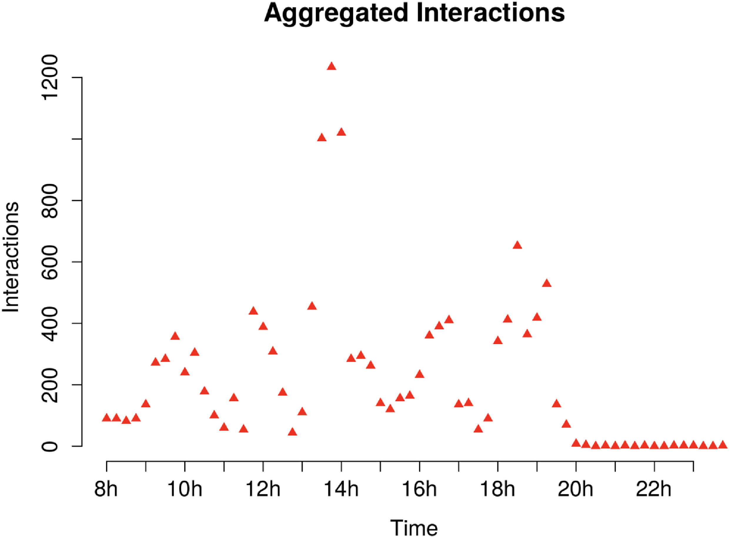
This interaction dataset was first analyzed by Isella et al. (Reference Isella, Stehlé, Barrat, Cattuto, Pinton and den Broeck2011) and is publicly available from Hypertext 2009 network dataset - KONECT (2017). Similarly to Corneli et al. (Reference Corneli, Latouche and Rossi2016), we focus our analysis on the first day of the conference. On the first day, the main events that took place included a poster session in the morning (starting from 8 a.m.), a lunch break around 1 p.m., and a cheese and wine reception in the evening between 6 and 7 p.m. (Figure 9).
ACM application: cumulative number of interactions for each quarter hour (first day).
We use our distance CLPM to provide a graphical representation of these data and to note how the model responds to the various gatherings that happened during the day. We use $20$
change points, which we found provided a sufficient level of flexibility for this application. Figures 10 and 11 show a number of snapshots highlighting some of the relevant moments of the day. The complete results, shown as a video, can be found in the code repository that accompanies this paper.
$20$
change points, which we found provided a sufficient level of flexibility for this application. Figures 10 and 11 show a number of snapshots highlighting some of the relevant moments of the day. The complete results, shown as a video, can be found in the code repository that accompanies this paper.
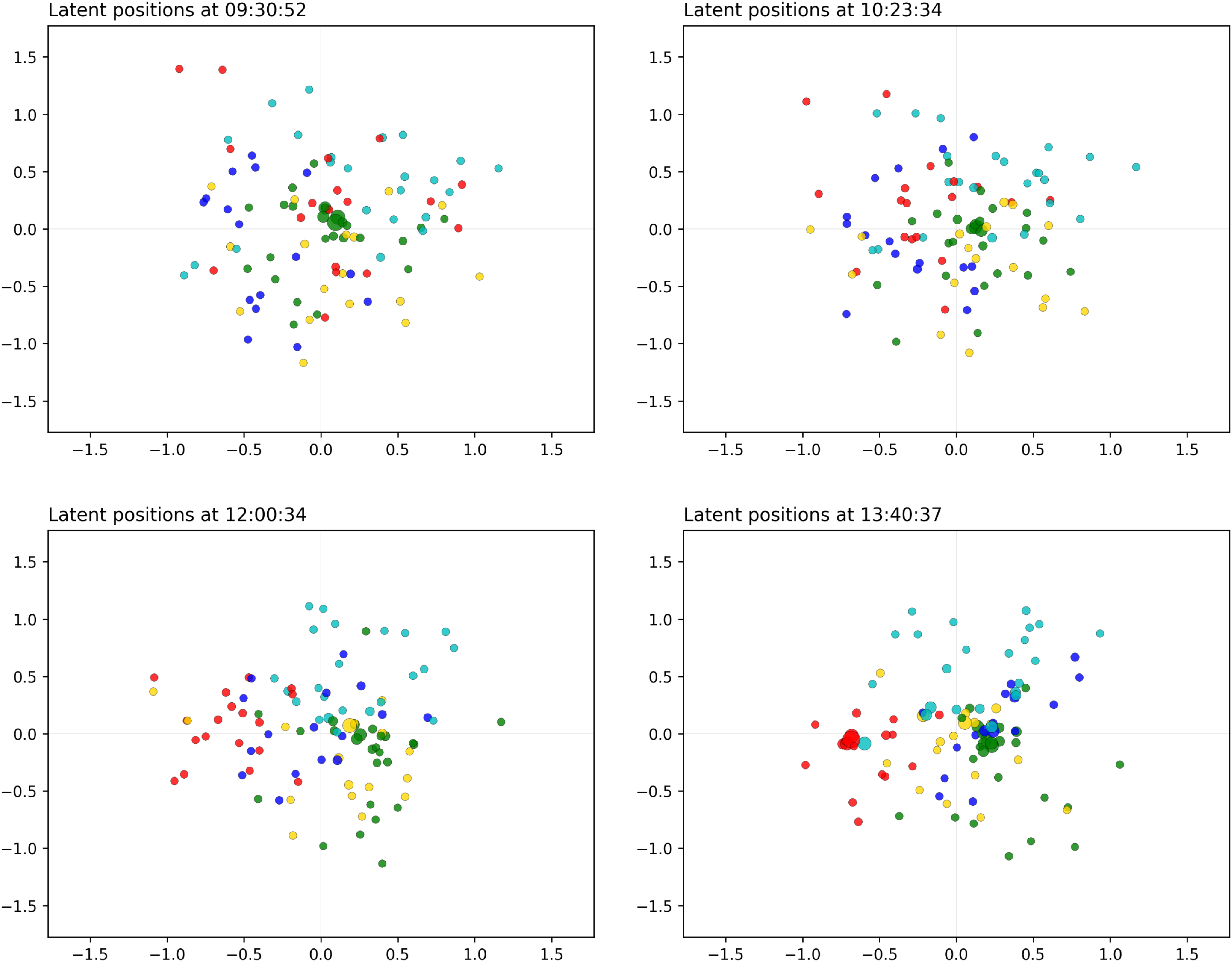
ACM application: snapshots for the distance model (morning hours). The sizes of the nodes reflect their current level of interaction. The colors are obtained with the spectral procedure of Section 4, with five groups.
ACM application: snapshots for the distance model (afternoon hours). The sizes of the nodes reflect their current level of interaction. The colors are obtained with the spectral procedure of Section 4, with five groups.
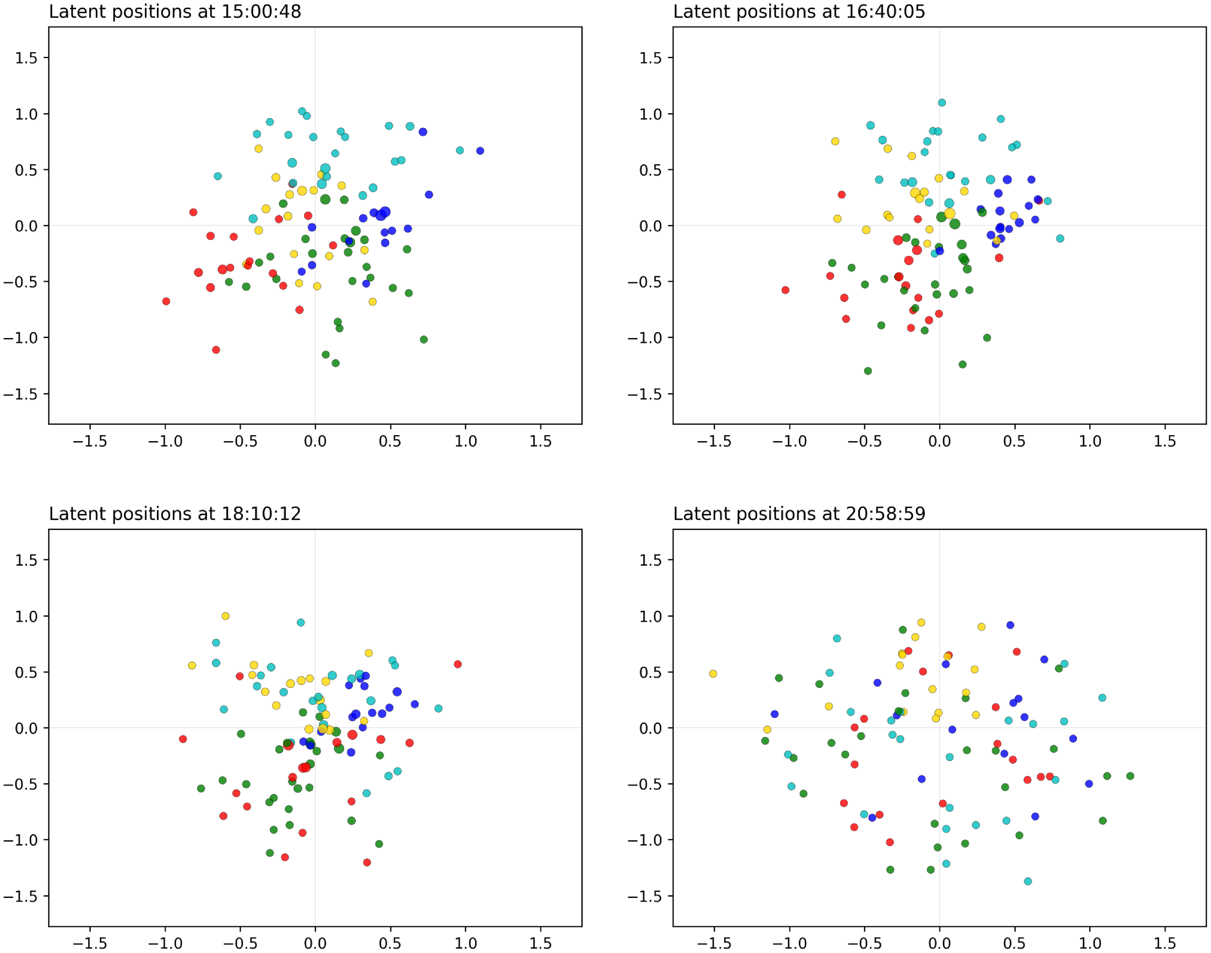
We can see that, in the morning, there is a high level of mixing between the attendees. The visitors tend to merge and split into different communities that change very frequently and very randomly. These communities reach a high level of clusteredness, which signals that the participants of the study are mixing into different groups. This is perfectly in agreement with the idea that the participants are moving from one location to another, as it usually happens during poster sessions and parallel talk sessions. The nodes exhibit different types of patterns and behaviors, in that some nodes are central and tend to join many communities, whereas others have lower levels of participation and remain at the outskirts of the space.
In the late morning, we see a clear close gathering around 12 p.m., whereby almost all nodes move toward the center of the space. This is emphasized even more at 1.40 p.m., which corresponds to the lunch break. It is especially interesting that, even though the space becomes more contracted at this time, we can still clearly see a strong clustering structure.
In the afternoon, we go back to the same patterns as in the morning, whereby the participants mix in different groups and move around the space. The wine reception is also clearly captured around 6 p.m. where we see again some level of contraction of the space, to signal a large gathering of the participants.
After this event, the overall rate of interactions diminishes sharply, and as a consequence we see the nodes spreading out in the space.
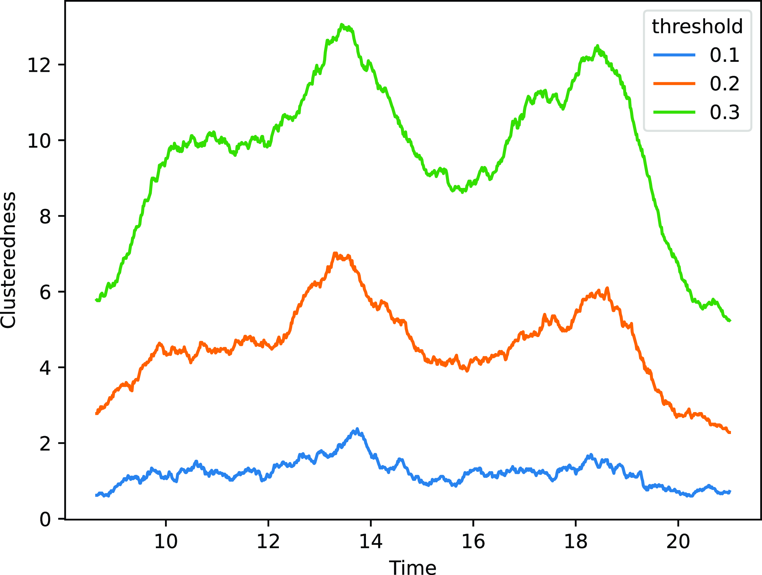
In terms of clustering, we use the index introduced in Section 4 on the results for the distance model, for various threshold levels. The results are shown in Figure 12, where we can appreciate strong time-dynamic patterns. All threshold values highlight several peaks for the clustering measure, confirming the aggregations happening throughout the morning, at lunchtime, and in the evening. In addition, we can also highlight a number of smaller cycles, which are congruent with the creation and dissolution of small communities as may be observed during parallel sessions or poster presentations.
ACM application: clusteredness measure for various threshold values. The x-axis shows the hour of the day, whereas the y-axis shows the average number of nodes that a random node would have within the threshold distance.
6.2 Reality mining
The reality mining dataset (Eagle and Pentland, Reference Eagle and Pentland2006) is derived from the Reality Commons project, which was run at the Massachusetts Institute of Technology from $14$
September 2004 to
$14$
September 2004 to $5$
May 2005. The dataset describes proximity interactions in a group of
$5$
May 2005. The dataset describes proximity interactions in a group of $96$
students, collected primarily through Bluetooth devices. An overview of this network dataset is also given by Rastelli (Reference Rastelli2019).
$96$
students, collected primarily through Bluetooth devices. An overview of this network dataset is also given by Rastelli (Reference Rastelli2019).
In the context of this paper, the proximity interactions can be reasonably considered as instantaneous interactions, due to the study being $9$
months long. With our latent space representation, we aim at highlighting the patterns of connections of the students during the study, and any social communities that arise and how these change over time.
$9$
months long. With our latent space representation, we aim at highlighting the patterns of connections of the students during the study, and any social communities that arise and how these change over time.
Figure 13 shows a few snapshots of our fitted distance CLPM. For this application, we also used $20$
change points; however, all the implementation details, along with the complete results shown as a video, can be found in the code repository that accompanies this paper.
$20$
change points; however, all the implementation details, along with the complete results shown as a video, can be found in the code repository that accompanies this paper.
MIT application: snapshots for the distance model. The sizes of the nodes reflect their current level of interaction. The colors are obtained with the spectral procedure of Section 4, with five groups.
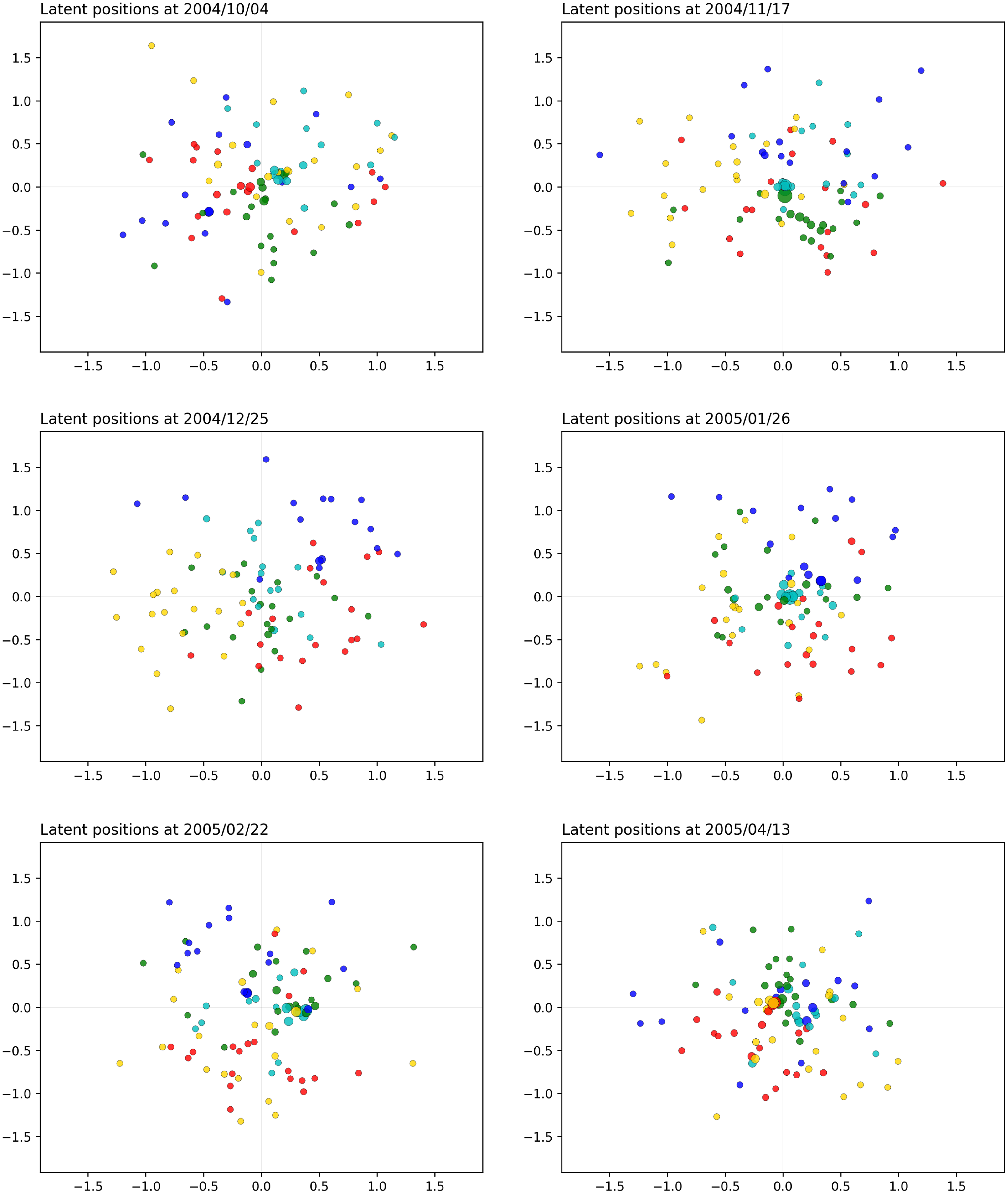
We observe that, in general, the students are quite separated and few communities arise. This does not necessarily mean that the nodes do not interact, but it is a sign that there are no subgroups of students with an uncommonly high interaction rate. Over time, the students tend to mix in different social groups, thus quickly forming and undoing communities. This could be explained by the interactions that the students have due to college activities or other daily activities. Near the end of the study, a large cluster appears, signaling a large gathering to which the students participated. This may correspond to the period before a deadline, as outlined in Eagle and Pentland (Reference Eagle and Pentland2006).
6.3 London bikes
Infrastructure networks provide an excellent example of instantaneous interaction data. In this section, we consider a network of bike hires which is collected and publicly distributed by Transport for London: Cycle hire usage data 2012–2015 (n.d.). We focus on a specific weekend day (Sunday 6 September 2015) and study the patterns of interactions between all bike hire stations in London over 24 h, from midnight to midnight. The bike hire stations correspond to the nodes of our network, whereas an instantaneous interaction between two nodes at time $t$
simply means that a bike started a journey from one station toward the other, at that time (we consider undirected connections). For the change points
$t$
simply means that a bike started a journey from one station toward the other, at that time (we consider undirected connections). For the change points $\eta _1, \ldots, \eta _K$
, we set a change point every 15 min, for a total
$\eta _1, \ldots, \eta _K$
, we set a change point every 15 min, for a total $K=96$
change points over the day.
$K=96$
change points over the day.
In Figure 14, we show a collection of snapshots at some critical time points during the day, for the distance model. Figure 15 shows instead the clusteredness index. The complete results, shown as a video, can be found in the code repository that accompanies this paper. Although there are a total of $818$
stations that are active in this dataset, we provide a visualization for the
$818$
stations that are active in this dataset, we provide a visualization for the $60$
most active stations only. However, we emphasize that the results were obtained using the whole dataset. As said, we highlight with a different color the three stations with the highest number of interactions, overall. These stations are:
$60$
most active stations only. However, we emphasize that the results were obtained using the whole dataset. As said, we highlight with a different color the three stations with the highest number of interactions, overall. These stations are:
London bikes application: snapshots for the distance model. The sizes and colors (fading from blue to yellow) of the nodes reflect their current level of interaction. Three most active stations are shown in red, green, and yellow.
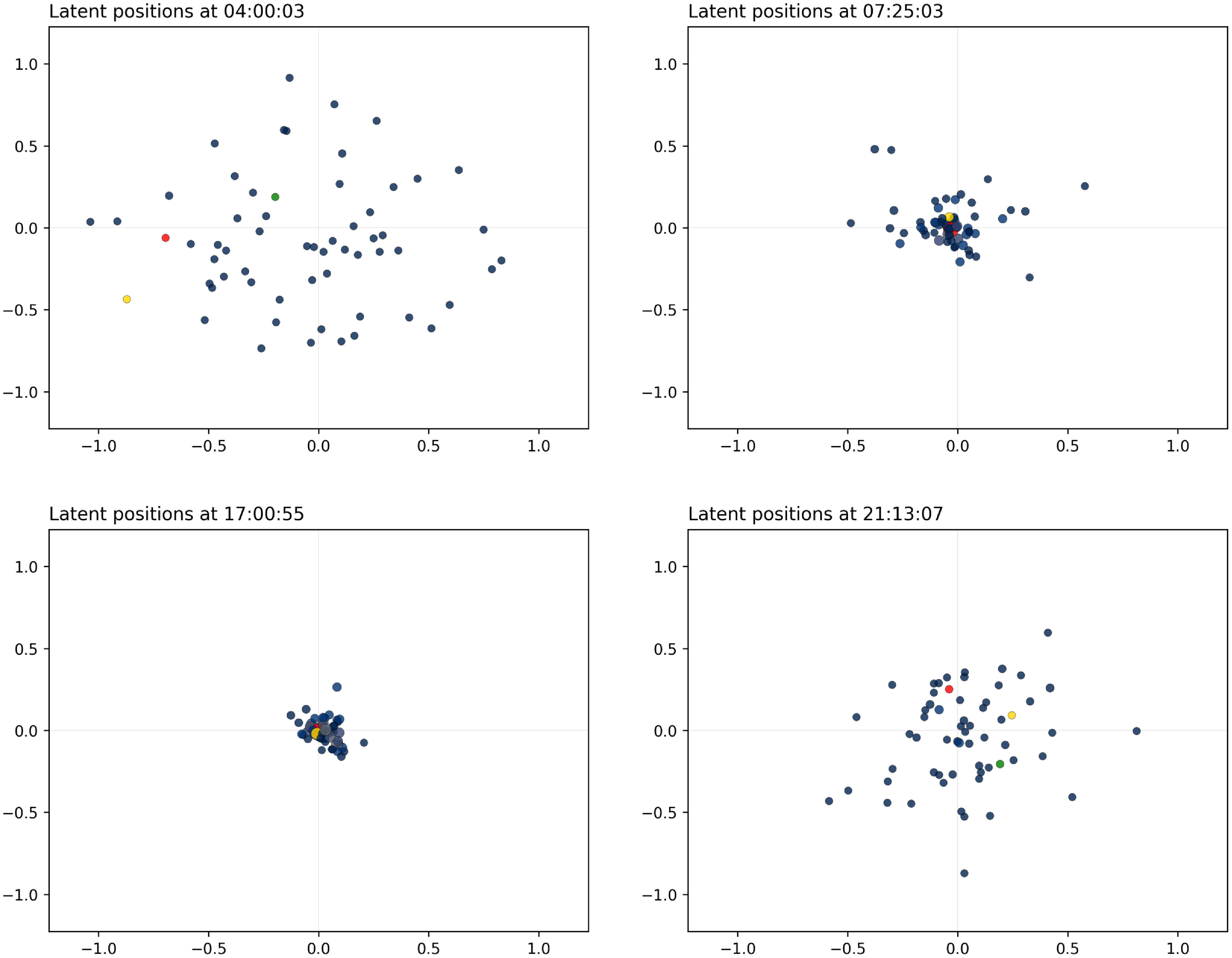
London bikes application: clusteredness measure for various threshold values. The x-axis shows the hour of the day, whereas the y-axis shows the average number of nodes that a random node would have within the threshold distance.
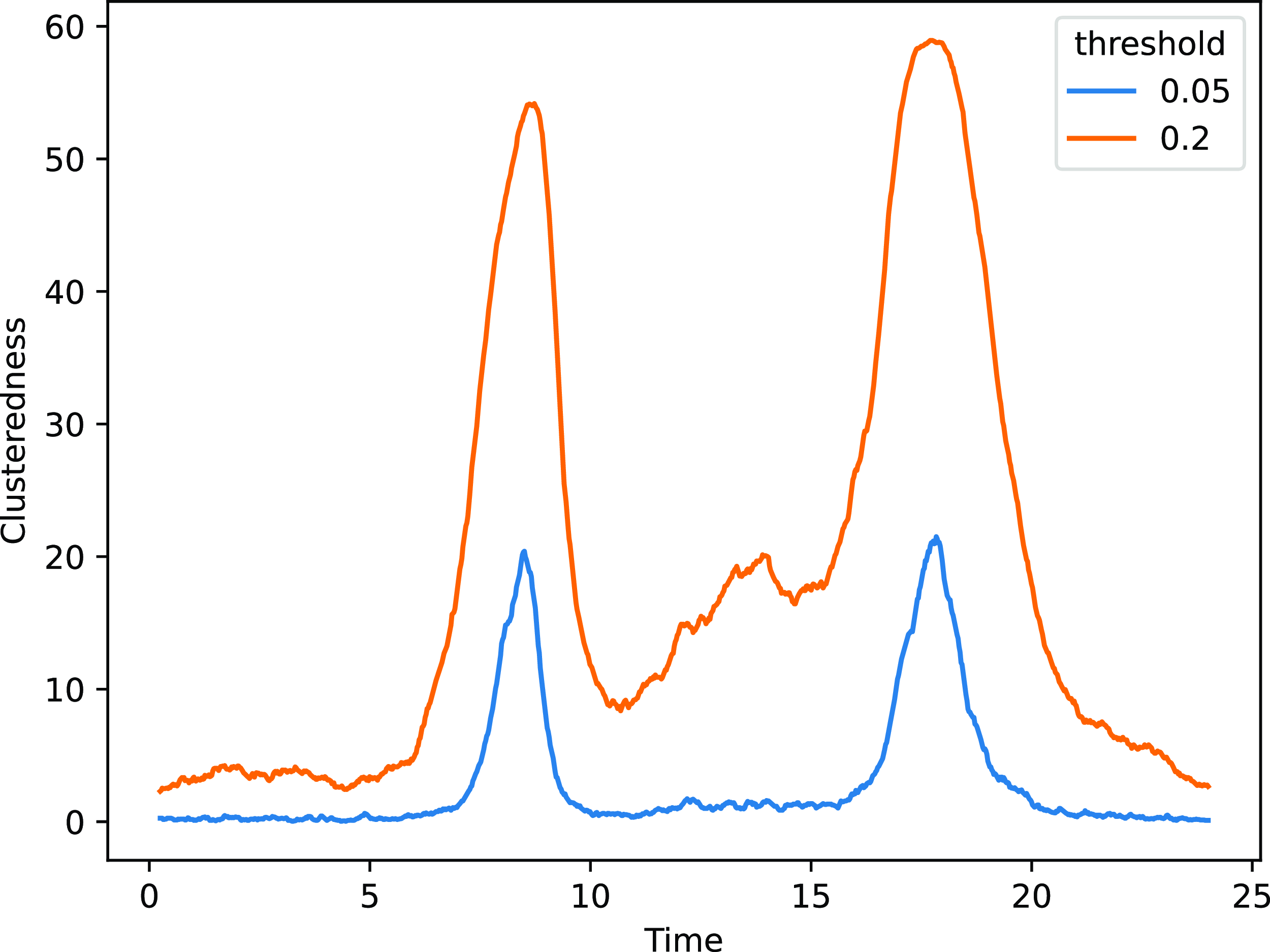
-
Belgrove Street, King’s Cross, situated next to King’s Cross Square (shown in red);
-
Finsbury Circus, Liverpool Street, situated next to Liverpool Street station (shown in green);
-
Newgate Street, St. Paul’s, situated next to St. Paul’s Cathedral (shown in yellow).
The first aspect that we notice is that the latent space expands during inactive times, and it contracts during busy hours. The contractions and expansions are not homogeneous; rather they highlight the presence of dense and less dense clusters of stations.
The estimate for the intercept parameter is $-4.95$
, and the dispersion of the points in the latent space is not particularly large. This indicates that the latent space characterization is not having a very strong effect on the rate of interactions, and the model does not capture much variability in the rates of interactions. This highlights that these connectivity data follow patterns that cannot be completely explained by the purely geometrical nature of our model. That is, the connections are determined by a variety of factors that cannot be framed into this latent position’s context, and the geographical information on bike hiring accounts for only a part of the problem.
$-4.95$
, and the dispersion of the points in the latent space is not particularly large. This indicates that the latent space characterization is not having a very strong effect on the rate of interactions, and the model does not capture much variability in the rates of interactions. This highlights that these connectivity data follow patterns that cannot be completely explained by the purely geometrical nature of our model. That is, the connections are determined by a variety of factors that cannot be framed into this latent position’s context, and the geographical information on bike hiring accounts for only a part of the problem.
7. Conclusions and perspectives
We have introduced a new time-continuous version of the well known and widely used LPM, as an extension which can model instantaneous interactions between entities. We have proposed a new methodology which provides good flexibility while also allowing for an efficient inferential framework. The methodology is implemented in our software CLPM which accompanies this paper and is publicly available. This provides an essential additional tool for practitioners that are interested in deriving latent space visualizations from observed instantaneous interaction data.
The framework that we propose is highly inspired by the work of Hoff et al. (Reference Hoff, Raftery and Handcock2002) and by the vast literature that has followed in this direction. Our work combines some crucial theoretical and statistical aspects of latent position modeling, with a pragmatic approach to inference and visualization of the results. Crucially, we provide simulation studies and real data applications to demonstrate how our method leads to sensible and accurate results, with low computational demands.
As regards extensions and future work, our research opens up several new directions, to address and potentially change some crucial parts of our procedure. Being able to assess the uncertainty around the estimated latent positions would be crucial, but it is not trivial. Indeed, as the observed data log-likelihood is invariant with respect to isometries in the latent space, sampling from the posterior distribution could lead to non-interpretable samples. For the very same reason, parametric bootstrap cannot be easily exploited. Stochastic variational inference seems to be the most valuable way to quantify the uncertainty around $Z$
. Another fundamental challenge is related to the geometric nature of the latent space. In this paper, and in the literature cited here, affine latent spaces are considered, endowed with the standard dot product, which, in turn, induces the Euclidean distance. However, some important works in the literature of the static LPM consider the latent space to be spherical (McCormick and Zheng, Reference McCormick and Zheng2015) or hyperbolic (Krioukov et al., Reference Krioukov, Papadopoulos, Kitsak, Vahdat and Boguná2010; Asta and Shalizi, Reference Asta and Shalizi2015). As expected, since LPMs are generative models, the geometry of the latent space has crucial consequences on the properties of the simulated network (Smith et al., Reference Smith, Asta and Calder2019). Indeed, recently, Lubold et al. (Reference Lubold, Chandrasekhar and McCormick2020) introduced a method to consistently estimate the manifold type, dimension, and curvature from a class of latent spaces. Addressing these topics in the context of dynamic LPMs is a promising avenue of research that can extend our work. Another challenging aspect of our methodology regards inference: in this paper, we propose an optimization approach to maximize a penalized likelihood. An interesting alternative would be to consider a different approach that could allow one to also quantify uncertainty around the parameter estimates. Goodness of fit and model selection is also another critical aspect of our proposed method. In this work, we have primarily focused on data visualization and interpretation as a goal. However, many modeling decisions that we have arbitrarily taken (e.g., number of latent dimensions, penalization parameter values) could be replaced by more formal procedures that rely on model choice criteria and goodness of fit. This opens up a number of interesting research directions that we leave as potential future work. Finally, in terms of modeling, we use piece-wise continuous trajectories due to their flexibility and easy tractability. However, the assumption of fixing the change points arbitrarily is a limitation of our framework, and so alternatives to our parametrization may be considered to allow the change points to be estimated from the data.
$Z$
. Another fundamental challenge is related to the geometric nature of the latent space. In this paper, and in the literature cited here, affine latent spaces are considered, endowed with the standard dot product, which, in turn, induces the Euclidean distance. However, some important works in the literature of the static LPM consider the latent space to be spherical (McCormick and Zheng, Reference McCormick and Zheng2015) or hyperbolic (Krioukov et al., Reference Krioukov, Papadopoulos, Kitsak, Vahdat and Boguná2010; Asta and Shalizi, Reference Asta and Shalizi2015). As expected, since LPMs are generative models, the geometry of the latent space has crucial consequences on the properties of the simulated network (Smith et al., Reference Smith, Asta and Calder2019). Indeed, recently, Lubold et al. (Reference Lubold, Chandrasekhar and McCormick2020) introduced a method to consistently estimate the manifold type, dimension, and curvature from a class of latent spaces. Addressing these topics in the context of dynamic LPMs is a promising avenue of research that can extend our work. Another challenging aspect of our methodology regards inference: in this paper, we propose an optimization approach to maximize a penalized likelihood. An interesting alternative would be to consider a different approach that could allow one to also quantify uncertainty around the parameter estimates. Goodness of fit and model selection is also another critical aspect of our proposed method. In this work, we have primarily focused on data visualization and interpretation as a goal. However, many modeling decisions that we have arbitrarily taken (e.g., number of latent dimensions, penalization parameter values) could be replaced by more formal procedures that rely on model choice criteria and goodness of fit. This opens up a number of interesting research directions that we leave as potential future work. Finally, in terms of modeling, we use piece-wise continuous trajectories due to their flexibility and easy tractability. However, the assumption of fixing the change points arbitrarily is a limitation of our framework, and so alternatives to our parametrization may be considered to allow the change points to be estimated from the data.
Acknowledgments
The authors would like to thank Prof. Charles Bouveyron for useful feedback in the early stages of this work and also for supporting and coordinating a research visit which fostered this project.
Funding
This research received no specific grant from any funding agency, commercial, or not-for-profit sectors.
Competing interests
None.
A. Log-likelihood for the projection model
To make the forthcoming results clearer, we introduce the following notation for the dot products:
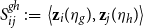 \begin{equation} S_{ij}^{gh} \,:\!=\, \left \langle \textbf{z}_i(\eta _g), \textbf{z}_j(\eta _h) \right \rangle \end{equation}
for some nodes $i$
and
$i$
and $j$
, and for any
$j$
, and for any $g,h \in \left \{1,\ldots,K\right \}$
. Most commonly,
$g,h \in \left \{1,\ldots,K\right \}$
. Most commonly, $g$
and
$g$
and $h$
will correspond to the labels of two consecutive change points; thus, we will use them to identify two breakpoints for the trajectories and to reconstruct the positions in between. Also, we denote:
$h$
will correspond to the labels of two consecutive change points; thus, we will use them to identify two breakpoints for the trajectories and to reconstruct the positions in between. Also, we denote:
 \begin{equation*}S_{ij}(t) \,:\!=\, \left \langle \textbf {z}_i(t), \textbf {z}_j(t) \right \rangle \end{equation*}
for the dot product at a generic time $t \in [0,T]$
.
$t \in [0,T]$
.
Proposition 2. Under the projection model, the log-likelihood is exactly equal to:
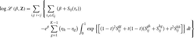 \begin{equation} \begin{split} \log \mathcal{L}\left (\beta, \textbf{Z}\right ) &= \sum _{i,j:\ i < j} \left \{ \sum _{\tau _e \in \mathcal{E}_{ij}} (\beta + S_{ij}(\tau _e)) \right . \\ &\hspace{1cm} \left .- e^\beta \sum _{g=1}^{K-1} \left (\eta _{h} - \eta _{g}\right )\int _{0}^{1} \exp \left \{\left [(1-t)^2S_{ij}^{gg} + t(1-t)(S_{ij}^{gh}+S_{ij}^{hg}) + t^2S_{ij}^{hh}\right ]\right \}dt \right \} \end{split} \end{equation}
where $h = g+1$
.
$h = g+1$
.
Proof. The only non-trivial part in formula (4) regards the integral:
 \begin{equation*} \int _{0}^{T} \exp \{\beta + \left \langle \textbf {z}_i(s), \textbf {z}_j(s) \right \rangle \}ds \end{equation*}
where we have that, for $s \in [\eta _g,\eta _{g+1}]$
:
$s \in [\eta _g,\eta _{g+1}]$
:
 \begin{equation*} \textbf {z}_i(s) = (1-t)\textbf {z}_i(\eta _g) + t\textbf {z}_i(\eta _{g+1}) \end{equation*}
and, thanks to Equation (3), $t \in [0,1]$
is such that
$t \in [0,1]$
is such that $s = (1-t)\eta _g + t\eta _{g+1}$
. Back to the calculation of the integral, we can decompose this into
$s = (1-t)\eta _g + t\eta _{g+1}$
. Back to the calculation of the integral, we can decompose this into $K-1$
integrals using the
$K-1$
integrals using the $K$
change points as follows:
$K$
change points as follows:
 \begin{equation*} {\int _{0}^{T} \exp \{\beta +\left \langle \textbf {z}_i(s), \textbf {z}_j(s) \right \rangle \}ds = e^\beta \sum _{g=1}^{K-1} \int _{\eta _g}^{\eta _{g+1}} \exp \{\left \langle \textbf {z}_i(s), \textbf {z}_j(s) \right \rangle \}ds} \end{equation*}
and then, in each integral, we apply the transformation $s = (1-t)\eta _g + t\eta _{g+1}$
and set
$s = (1-t)\eta _g + t\eta _{g+1}$
and set $h = g+1$
to obtain:
$h = g+1$
to obtain:
 \begin{align*} \begin{split} \int _{\eta _g}^{\eta _h} \exp \{\left \langle \textbf{z}_i(s), \textbf{z}_j(s) \right \rangle \}ds &= \left (\eta _{h} - \eta _g\right )\int _{0}^{1} \exp \left \{\left \langle \textbf{z}_i((1-t)\eta _g+t\eta _{h}), \textbf{z}_j((1-t)\eta _g+t\eta _{h}) \right \rangle \right \}dt \\ &= \left (\eta _{h} - \eta _g\right )\int _{0}^{1} \exp \left \{\left [(1-t)^2S_{ij}^{gg} + t(1-t)(S_{ij}^{gh}+S_{ij}^{hg}) + t^2S_{ij}^{hh}\right ]\right \}dt \end{split} \end{align*}
where $S_{ij}^{gh}$
is defined in Equation (A1). Since the
$S_{ij}^{gh}$
is defined in Equation (A1). Since the $S$
terms do not depend on
$S$
terms do not depend on $t$
, the integral can be efficiently approximated using a composite Simpson’s rule (see equation
$t$
, the integral can be efficiently approximated using a composite Simpson’s rule (see equation $5.1.16$
of Atkinson (Reference Atkinson1991)).
$5.1.16$
of Atkinson (Reference Atkinson1991)).
B. Log-likelihood for the distance model
We focus on the integral in Equation (6) and prove that it can be explicitly solved.
Proof. In force of Equation (3), it reads
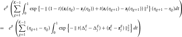 \begin{equation} \begin{split} &e^{\beta }\left (\sum _{g=1}^{K-1}\int _{0}^{1} \exp \left \{-\parallel (1-t)(\textbf{z}_i(\eta _g) - \textbf{z}_j(\eta _g)) + t(\textbf{z}_i(\eta _{g+1})-\textbf{z}_{j}(\eta _{g+1})) \parallel ^2\right \} (\eta _{g+1} - \eta _{g}) dt \right ) \\ =&\quad e^{\beta }\left (\sum _{g=1}^{K-1}(\eta _{g+1} - \eta _{g}) \int _{0}^{1} \exp \left \{ - \parallel t (\Delta _i^g - \Delta _j^g) + (\textbf{z}_i^g - \textbf{z}_j^g) \parallel _2^2 \right \} dt \right ) \end{split} \end{equation}
where the variable change $t = \frac{s-\eta _g}{\eta _{g+1}-\eta _g}$
was performed and the following notations were adopted to simplify the exposition
$t = \frac{s-\eta _g}{\eta _{g+1}-\eta _g}$
was performed and the following notations were adopted to simplify the exposition
 \begin{align*} \begin{split} \Delta _i^g :&= \textbf{z}_i(\eta _{g+1}) - \textbf{z}_i(\eta _{g}) \\ \Delta _j^g :&= \textbf{z}_j(\eta _{g+1}) - \textbf{z}_j(\eta _{g}) \\ \textbf{z}_i^g :&= \textbf{z}_i(\eta _g) \\ \textbf{z}_j^g :&= \textbf{z}_j(\eta _g) \end{split} \end{align*}
By denoting $f(t)\,:\!=\,- \parallel t (\Delta _i^g - \Delta _j^g) + (\textbf{z}_i^g - \textbf{z}_j^g) \parallel _2^2$
the exponent inside the integral, we can “complete the square” as follows
$f(t)\,:\!=\,- \parallel t (\Delta _i^g - \Delta _j^g) + (\textbf{z}_i^g - \textbf{z}_j^g) \parallel _2^2$
the exponent inside the integral, we can “complete the square” as follows
 \begin{align*} \begin{split} f(t) &=-\parallel \Delta _i^g - \Delta _j^g \parallel ^2\left (t^2 + 2t\left \langle \frac{\Delta _i^g - \Delta _j^g}{\parallel \Delta _i^g - \Delta _j^g \parallel }, \frac{\textbf{z}_i^g - \textbf{z}_j^g}{\parallel \Delta _i^g - \Delta _j^g \parallel } \right \rangle + \frac{\parallel \textbf{z}_i^g - \textbf{z}_j^g \parallel ^2}{\parallel \Delta _i^g - \Delta _j^g \parallel ^2} \right ) \\ &=-\parallel \Delta _i^g - \Delta _j^g \parallel ^2\left (t - \left \langle \frac{\Delta _i^g - \Delta _j^g}{\parallel \Delta _i^g - \Delta _j^g \parallel }, \frac{\textbf{z}_j^g - \textbf{z}_i^g}{\parallel \Delta _i^g - \Delta _j^g \parallel } \right \rangle \right )^2 \\ &- \left (\parallel \textbf{z}_i^g - \textbf{z}_j^g \parallel ^2 - \left (\left \langle \frac{\Delta _i^g - \Delta _j^g}{\parallel \Delta _i^g - \Delta _j^g \parallel }, \textbf{z}_j^g - \textbf{z}_i^g \right \rangle \right )^2 \right ) \\ &= -\frac{1}{2(\sigma ^2)_{ij}^g}(t - \mu _{ij})^2 - \left (\parallel \textbf{z}_i^g - \textbf{z}_j^g \parallel ^2 - (\parallel \Delta _i^g - \Delta _j^g \parallel \mu _{ij}^g)^2 \right ) \end{split} \end{align*}
where
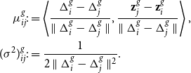 \begin{equation} \begin{split} \mu _{ij}^g :&= \left \langle \frac{\Delta _i^g - \Delta _j^g}{\parallel \Delta _i^g - \Delta _j^g \parallel }, \frac{\textbf{z}_j^g - \textbf{z}_i^g}{\parallel \Delta _i^g - \Delta _j^g \parallel } \right \rangle, \\ (\sigma ^2)^g_{ij} :&=\frac{1}{2\parallel \Delta _i^g - \Delta _j^g \parallel ^2}. \end{split} \end{equation}
By plugging all this into Equation (B1), it follows that
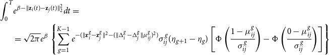 \begin{equation} \begin{split} \int _0^T & e^{\beta - \parallel \textbf{z}_{i}(t) - \textbf{z}_{j}(t) \parallel _2^2} dt = \\ &=\sqrt{2\pi } e^{\beta }\left \{\sum _{g=1}^{K-1}e^{-(\parallel \textbf{z}_i^g - \textbf{z}_j^g \parallel ^2 - (\parallel \Delta _i^g - \Delta _j^g \parallel \mu _{ij}^g)^2 )} \sigma _{ij}^g (\eta _{g+1} - \eta _g) \left [\Phi \left (\frac{1-\mu _{ij}^g}{\sigma _{ij}^g}\right )- \Phi \left (\frac{0-\mu _{ij}^g}{\sigma _{ij}^g}\right )\right ] \right \} \end{split} \end{equation}


 Open access