


INTRODUCTION
The Taiwanese tablelands
The island of Taiwan is located at the convergence zone of the Eurasian and the Philippine Sea plates; it has been continuously uplifted since the late Tertiary (e.g., Suppe, Reference Suppe1981; Teng, Reference Teng1990; Fig. 1a). The central mountain ranges reach altitudes above 3500 m in several massifs and are built up of pre-Miocene to Pliocene metamorphic rocks (Chang, Reference Chang1953, Reference Chang1955a; Ho, Reference Ho1988). Their western fringes are called the Western Foothills (WF) (Angelier et al., Reference Angelier, Barrier and Chu1986; Ho, Reference Ho1988).
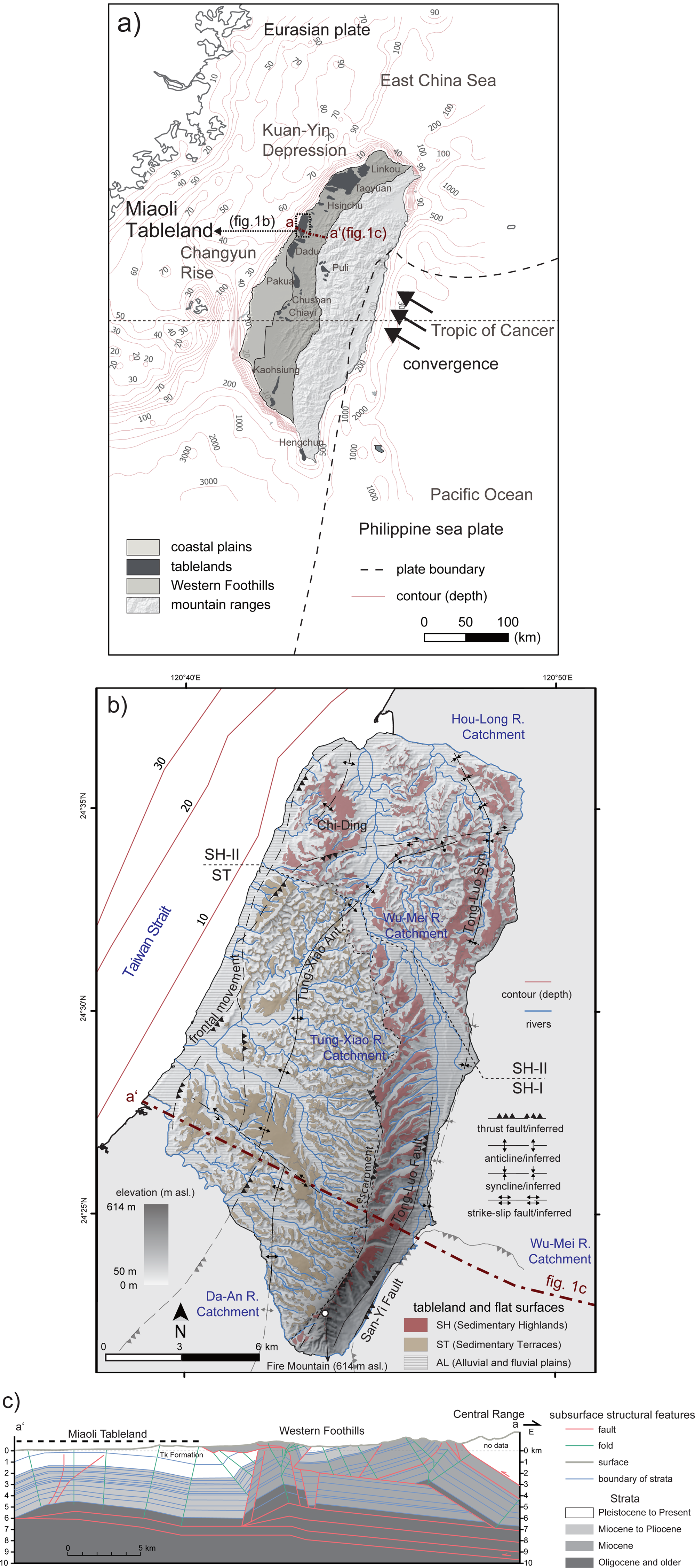
Figure 1. (a) Location of Taiwan and the tablelands in the regional tectonic context (simplified from Suppe [Reference Suppe1984], Angelier et al. [Reference Angelier, Barrier and Chu1986], and Ho [Reference Ho1988]); the bathymetry of the Taiwan Strait was simplified from Jan et al. (Reference Jan, Wang, Chern and Chao2002). (b) The Miaoli Tableland and its subdivision into three morphological units from east to west. The elevation data are simplified from the open-access digital elevation model (DEM) with 20 m resolution (Satellite Survey Center, 2018). Tectonic situation based on a simplification of the online database of geologic maps (Central Geological Survey, 2017); the Tung-Luo Thrust Fault was identified by Ota et al. (Reference Ota, Lin, Chen, Chang and Hung2006); the inferred thrust at the escarpment in between the Sedimentary Highlands located to the west of the Tung-Luo Thrust Fault (SH-I) and Sedimentary Terraces (ST) by Chang et al. (Reference Chang, Teng and Liu1998); the “frontal movement” is simplified from Shyu et al. (Reference Shyu, Sieh, Chen and Liu2005). (c) The underground geologic structure from the Western Foothills (WF) to the Miaoli Tableland and its surrounding area of the WF (simplified from Yang et al., Reference Yang, Rau, Chang, Hsieh, Ting, Huang, Wu and Tang2016).
Tablelands represent characteristic landforms in Taiwan consisting of sedimentary terraces of different altitude, composition, and age. They are distributed mainly in the western mountain foreland (Tomita, Reference Tomita1940; Lin, Reference Lin1957; Lin and Chou, Reference Lin and Chou1974; Teng, Reference Teng1996; Fig. 1a), where they are composed of intercalating Quaternary tidal/coastal fine-grained sediments and are covered by fluvial gravels and cobbles yielded from the central orogenic belt (Lin, Reference Lin1957; Teng, Reference Teng1996). Variations in the yield of these coarse-grained sediments have been attributed to climatic changes (Huang et al., Reference Huang, Liew, Zhao, Chang, Kuo, Chen, Wang and Zheng1997; Tseng et al., Reference Tseng, Wenske, Böse, Reimann, Lüthgens and Frechen2013), that is, glacial and periglacial conditions in the high mountain ranges (Klose, Reference Klose2006; Hebenstreit et al., Reference Hebenstreit, Ivy-Ochs, Kubik, Schlüchter and Böse2011) or variable mass-wasting activity in the mountain catchments (Hsieh and Chyi, Reference Hsieh and Chyi2010). Tablelands are also present in an intramountainous basin (Puli Tableland), where they are composed of gravels and cobbles (Teng, Reference Teng1979; Teng, Reference Teng1996; Tseng et al., Reference Tseng, Wenske, Böse, Reimann, Lüthgens and Frechen2013, Reference Tseng, Lüthgens, Tsukamoto, Reimann, Frechen and Böse2016). The sedimentary successions can reach more than 1000 m in thickness in the western forelands. In central Taiwan, they are ascribed to the Toukoshan Formation (Chang, Reference Chang1955b; Ho, Reference Ho1988), which includes the underlying bedrock (Fig. 1c).
The tablelands were tectonically uplifted, partly tilted, and subsequently dissected by fluvial incision, resulting in an irregular topography of the respective tableland surfaces (Hsieh and Knuepfer, Reference Hsieh and Knuepfer2001; Simoes and Avouac, Reference Simoes and Avouac2006; Ota et al., Reference Ota, Lin, Chen, Matsuta, Watanuki and Chen2009; Siame et al., Reference Siame, Chen, Derrieux, Lee, Chang, Bourlès, Braucher, Léanni, Kang, Chang and Chu2012; Fox et al., Reference Fox, Goren, May and Willett2014).
The bathymetry of the Taiwan Strait (Jan et al., Reference Jan, Wang, Chern and Chao2002) indicates that Pleistocene sea-level lowering during glacial periods resulted in shoreline progradation and emergence of a land bridge (Liu et al., Reference Liu, Xia, Berne, Wang, Marsset, Tang and Bourillet1998; Hsieh et al., Reference Hsieh, Lai, Wu, Lu and Liew2006; Bradley et al., Reference Bradley, Milne, Horton and Zong2016; Fig. 1a). The drop in base level also influenced the balance of sedimentation and incision in the Taiwanese mountain foreland.
Previous interpretations of the tablelands’ chronology were based on proxies such as the lithification characteristics of the sedimentary strata, the degree of weathering of surface sediments and elevation differences. The tablelands were grouped into Lateritic Highlands (oldest), Lateritic Terraces (intermediate), and Fluvial Terraces (youngest) (Tomita, Reference Tomita1951, Reference Tomita1953, Reference Tomita1954; Lin, Reference Lin1957). Various studies attempted to provide detailed chronological control for the tableland formation by using different dating methods. Radiocarbon dating of tableland surfaces in western-central Taiwan delivered depositional ages younger than 30 ka (Lin, Reference Lin1969; Hsieh and Knuepfer, Reference Hsieh and Knuepfer2001; Ota et al., Reference Ota, Shyu, Chen and Hsieh2002). Electron-spin resonance dating of mollusks in the tableland sediments in southern Taiwan gave depositional age estimates around 140–90 ka (Shih et al., Reference Shih, Sato, Ikeya, Liew and Chien2002), generally pointing toward deposition during Marine Oxygen Isotope Stage (MIS) 5 (Lisiecki and Raymo, Reference Lisiecki and Raymo2005; Cohen et al., Reference Cohen, Harper and Gibbard2020). Depth profiles of cosmogenic 10Be on the surfaces the Pakua Tableland and other tablelands in northwest Taiwan delivered ages of up to 300 ka (Tsai et al., Reference Tsai, Maejima and Hseu2008; Siame et al., Reference Siame, Chen, Derrieux, Lee, Chang, Bourlès, Braucher, Léanni, Kang, Chang and Chu2012). Luminescence dating of tableland sediments in north (Hsinchu area) and central (Pakua and Chushan areas) Taiwan yielded Pleistocene ages from 340 ± 66 to 13.5 ± 2.5 ka (Chen et al., Reference Chen, Chen, Chen, Zhang, Zhao, Zhou and Li2003a, Reference Chen, Chen, Chen, Lee, Lee, Lu, Lee, Watanuki and Lin2009; Simoes et al., Reference Simoes, Avouac, Chen, Singhvi, Wang, Jaiswal, Chan and Bernard2007; Ota et al., Reference Ota, Lin, Chen, Matsuta, Watanuki and Chen2009; Le Béon et al., Reference Le Béon, Suppe, Jaiswal, Chen and Ustaszewski2014).
Geomorphological and sedimentological setting of the Miaoli Tableland
The Miaoli Tableland (called “Miaoli Hills” in earlier morphological studies; Chang et al., Reference Chang, Teng and Liu1998) is located on the western coast of Taiwan between the Hou-Long River and the Da-An River. To the east it is bounded by the Tung-Luo Thrust Fault (Fig. 1b). The spatial extent of the tableland is about 28 km from north to south and about 14 km from east to west (Fig. 1b). The highest elevations are found at Fire Mountain (614 m above sea level [m asl]) at the southeastern edge of the tableland.
The topography of the Miaoli Tableland is characterized by a deep and narrowly spaced fluvial dissection into numerous segments (Teng, Reference Teng1979; Chang et al., Reference Chang, Teng and Liu1998) and their remnants (Liu et al., Reference Liu, Hebenstreit and Böse2022). Based on geomorphological studies (Liu et al., Reference Liu, Hebenstreit and Böse2022), these segments were categorized into three subgroups according to their position relative to one another, elevation, and morphology (Figs. 1b and 2). The Sedimentary Highlands (SH) can be subdivided into SH-I, located to the west of the Tung-Luo Thrust Fault, and SH-II, the northern part on both sides of the Wu-Mei River (Fig. 1b). The Sedimentary Terraces (ST) are located in the central and southwestern part of the Miaoli Tableland, that is, they are distributed across the whole Tung-Xiao River catchment. Except for the tableland segments and their remnants, all other surfaces below 150 m asl, which are active fluvial plains in the valley floors and coastal plains, are grouped into the Alluvial and Coastal plains (AL) (Fig. 1b). The degree of weathering and colors of surface sediments of the tableland segments have shown a correlation: surfaces of the larger segments are highly weathered with reddish-ocher soils (up to 1.5 m thick); the smaller segments, the remnants, and the downslope surfaces show moderately weathered, light reddish-yellowish soils of normally less than 1 m thickness (Chen, Reference Chen1983). A similar correlation based on pedological charateristics, relative chronology, and tableland morphology was published for the nearby (12 km south) Dadu Tableland (Tsai et al., Reference Tsai, Hseu, Huang, Huang and Chen2010) and (30 km south) Pakua Tableland (Siame et al., Reference Siame, Chen, Derrieux, Lee, Chang, Bourlès, Braucher, Léanni, Kang, Chang and Chu2012).
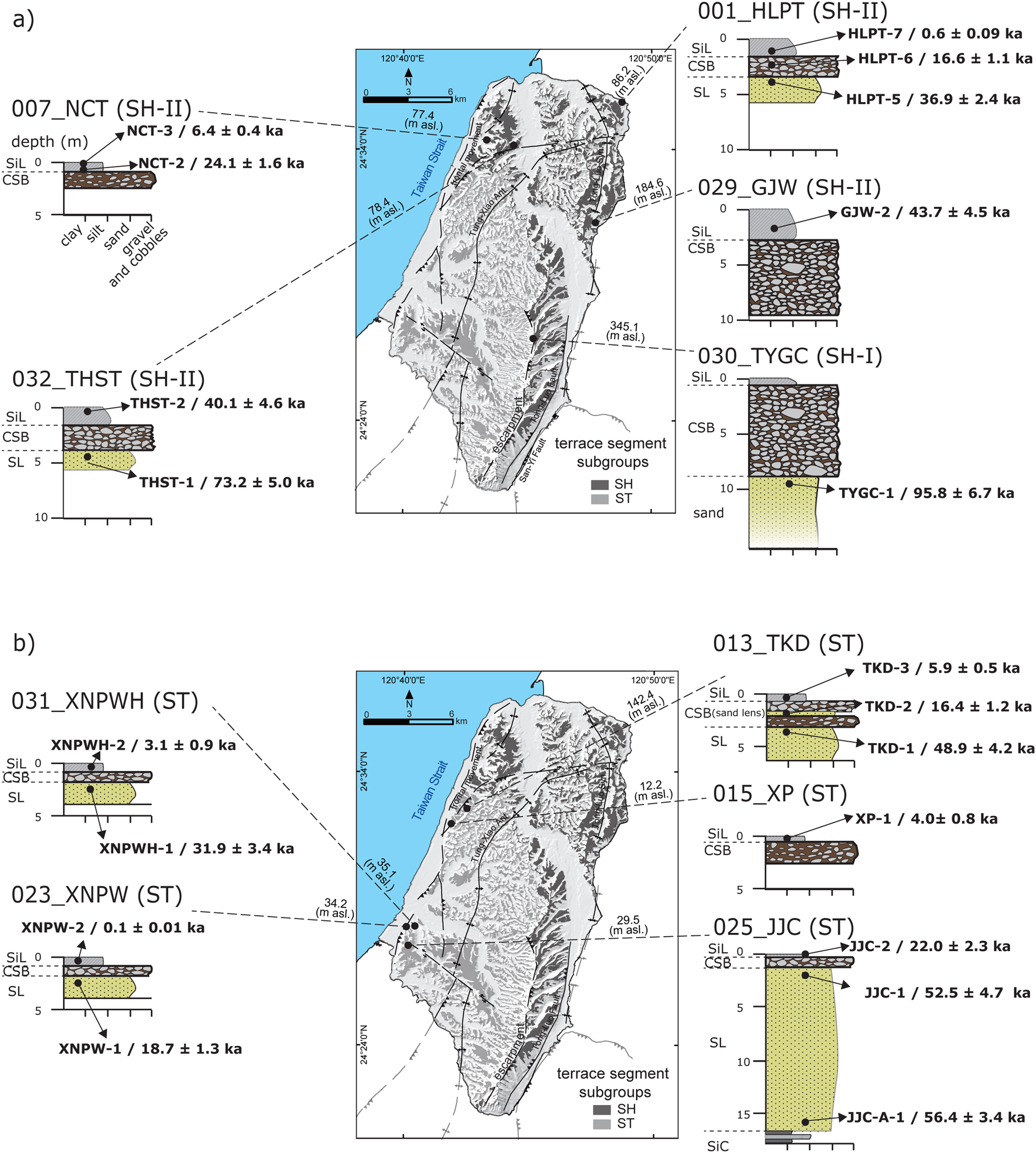
Figure 2. Locations, schematic profiles of the 10 outcrops dated in this study and the derived optically simulated luminescence (OSL) ages (a) in the Sedimentary Highlands (SH-I in the southeast and SH-II in the north and northwest) and (b) the Sedimentary Terraces (ST). The sampling locations for the OSL analyses are highlighted (see Table 2 for detailed information). The nomenclature of the sedimentary units follows Liu et al. (Reference Liu, Hebenstreit and Böse2022). SL, sandy loam; CSB, coarse sand with stones and boulders (gravels and cobbles); and SiL, silty loam (cover layer).
The sedimentary successions within the tableland segments vary between the subgroups (Liu et al., Reference Liu, Hebenstreit and Böse2022). SH-I, which is the highest and the oldest subgroup according to its degree of weathering, is composed of layers of gravels and cobbles, with an exposed thickness of ca. 300 m on Fire Mountain. In the SH-II and ST segments, which are less elevated and less weathered subgroups of the tableland morphology, the gravels and cobbles are distributed in comparably thin beds with thicknesses of <20 and <10 m, respectively and only <2 m in the distal areas of the tableland.
The non-uniform spatial distribution and the varying thickness of the gravel and cobble beds were interpreted by Liu et al. (Reference Liu, Hebenstreit and Böse2022) as an indicator of redepositions of the gravels and cobbles varying in space and time: a previously continuous distribution of the gravels and cobbles in the form of alluvial fans in the mountain foreland was reconstructed through high-resolution topographic analysis following the interpretation of Chang et al. (Reference Chang, Teng and Liu1998). After initial uplift, these gravels and cobbles were partly redistributed westward into the present ST area, forming a secondary continuous surface of a thin gravel and cobble bed. Further uplift and fluvial incision also dissected the ST into segments. The gravels and cobbles were thereby eroded from most of the segments, leaving only remnants of material (Liu et al., Reference Liu, Hebenstreit and Böse2022). The eroded gravels and cobbles were again redeposited farther downstream (Fig. 1b).
The sediments underlying the gravels and cobbles in the SH-II and the ST consist of fine-grained, loose sand and silt. Based on previous investigations in the Miaoli Tableland, they can be described as the Lungkang Formation—a generalized regression succession of tidal/ coastal sediments with an exposed thickness of up to 100 m (Makiyama, Reference Makiyama1936, Reference Makiyama1937; Lin, Reference Lin1963). Liu et al. (Reference Liu, Hebenstreit and Böse2022) described the sedimentary succession of the Miaoli Tableland, visible in outcrops, from bottom to top by using the international guidelines of soil descriptions (Jahn et al., Reference Jahn, Blume, Asio, Spaargaren and Schad2006): clay loam (L); sandy loam (LS); alternation of sandy loam and clay loam (SiC); and another layer of sandy loam (SL), buried by gravels and cobbles (coarse sand, with stones and boulders; CSB), and a cover layer of silty loam (SiL). The same succession of these layers was observed in broad areas of the SH-II and ST segments. The boundaries in between these sedimentary layers are very distinct (Liu et al., Reference Liu, Hebenstreit and Böse2022; Supplementary Appendix A), except where the gravel and cobble layer (CSB) is eroded and the silty loam layer (SiL) has direct contact with the sandy loam layer (SL).
The tableland segments were unevenly uplifted. Both the eastern and western margins of the SH-I segments are distinct topographic divides forming escarpments to the neighboring areas (Fig. 1b). A thrust fault has been defined in the eastern escarpment of the Sedimentary Highland area (Ota et al., Reference Ota, Lin, Chen, Chang and Hung2006) and another thrust fault was inferred at the western escarpment (Fig. 1b). The central areas of the SH-II and ST are the location of the Tung-Xiao Anticline. The latest thrust movement (tentatively called “frontal movement” by Shyu et al. [Reference Shyu, Sieh, Chen and Liu2005]) is located in the coastal areas (Fig. 1b). It has caused the topographic separation of the tableland segments and the coastal plains (Chang, Reference Chang1990, Reference Chang1994; Ho, Reference Ho1994; Lee, Reference Lee2000); the precise chronology of the movement is still unclear due to a lack of direct dating results.
The purpose of this study
So far, little is known about the timing of sediment deposition in the Miaoli Tableland, and uplift rates are poorly constrained. An early application of radiocarbon dating on mollusks from the fine-grained tidal sediments resulted in a Holocene age (Lin, Reference Lin1969), while later radiocarbon dating of the mollusks from the “Kuokang Shell Bed” yielded depositional ages between 45 and 31 ka (Wang and Peng, Reference Wang and Peng1990). Wang and Peng (Reference Wang and Peng1990) calculated an average uplift rate of 2 mm/yr on the basis of the vertical displacement of the dated mollusks. Biostratigraphic analyses of the microfossils from the fine-grained tidal sediments of the tableland segments suggested the overall age of the sediments was younger than 2.0 Ma (Lee et al., Reference Lee, Huang, Shieh and Chen2002). However, the stratigraphic context of all three aforementioned age estimations is unclear. Ota et al. (Reference Ota, Lin, Chen, Chang and Hung2006) assume an age of the highest terraces in the SH-I (“Sanyi Tableland”) older than 90 ka based on the degree of surface weathering in comparison with other tablelands (Ota et al., Reference Ota, Shyu, Chen and Hsieh2002).
The age of the gravel and cobble layers (CSB) in the Miaoli Tableland is still unknown, although the timing of their deposition and their uplift is essential for understanding the temporal evolution of the landscape and the formation of the Miaoli Tableland. Therefore, this study focuses on the age determination of the upper layers of the sedimentary succession mainly in the northern part of the Sedimentary Highlands (SH-II) and the Sedimentary Terraces (ST) by means of optically simulated luminescence (OSL). The results are used to infer uplift rates in the respective areas.
The successful application of luminescence dating has been demonstrated in several sedimentary environments and areas in Taiwan to determine the depositional ages of poorly lithified, quartz-rich sediments on Holocene and Pleistocene timescales (e.g., in the tablelands; Chen et al., Reference Chen, Chen, Chen, Zhang, Zhao, Zhou and Li2003a, Reference Chen, Chen, Chen, Lee, Lee, Lu, Lee, Watanuki and Lin2009; Chen et al., Reference Chen, Chen, Murray, Liu and Lai2003b; Le Béon et al., Reference Le Béon, Suppe, Jaiswal, Chen and Ustaszewski2014) as well as on cover sediments in high mountain areas (Hebenstreit et al., Reference Hebenstreit, Böse and Murray2006; Wenske et al., Reference Wenske, Böse, Frechen and Lüthgens2011, Reference Wenske, Frechen, Böse, Reimann, Tseng and Hoelzmann2012). In general, luminescence dating in Taiwan has proven to be challenging, especially when using quartz as a dosimeter. Quartz signals have been shown to be rather dim, in worst cases even rendering successful dating applications impossible, so feldspar has been used as a dosimeter instead (Ho et al., Reference Ho, Lüthgens, Wong, Yen and Chyi2017). Another frequently encountered issue is feldspar contamination of quartz that cannot be eliminated by repeated etching of the quartz separates in the preparation process. As a consequence, Dörschner et al. (Reference Dörschner, Reimann, Wenske, Lüthgens, Tsukamoto, Frechen and Böse2012) compared different approaches to circumvent this issue and tested post–IR-OSL (post–infrared stimulated optically stimulated luminescence) and pulsed-OSL protocols, finally opting for pulsed OSL, an approach later adopted by Tseng et al. (Reference Tseng, Wenske, Böse, Reimann, Lüthgens and Frechen2013). However, Lüthgens et al. (Reference Lüthgens, Ho, Clemenz, Chen, Jen, Yen and Chyi2018) demonstrated that continuous-wavelength OSL (CW-OSL) may also yield reliable luminescence ages, which were confirmed by comparison with feldspar-based luminescence ages as well as radiocarbon dating.
METHODS AND MATERIALS
Basic principles of luminescence dating
All luminescence dating approaches are based on determining a dosimeter's (e.g., quartz, feldspar mineral grains) last exposure to daylight. The basic luminescence age calculation is expressed by the equation (Aitken, Reference Aitken1985):

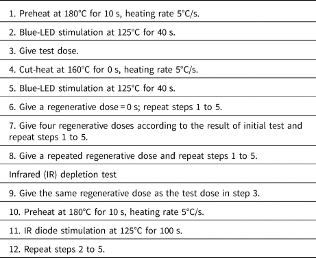
where D e is the equivalent dose, which is the radiation absorption by the dosimeter during the burial period; D r is the dose rate of environmental radiation. The radiation dose is given in grays (Gy). Luminescence dating can be applied to quartz grains (OSL) and potassium-rich feldspar grains (infrared stimulated luminescence [IRSL]) (Aitken, Reference Aitken1985). The application range of quartz OSL depends on the physical characteristics of the quartz grains. An applicational maximum D e is related to the dose saturation characteristics. The most common dose range (saturation limit) empirically observed and confirmed by laboratory and modeling experiments for quartz OSL ranges up to ca. 150 Gy, as stated and summarized in multiple studies (e.g., Jain et al., Reference Jain, Bøtter-Jensen, Murray, Denby, Tsukamoto and Gibling2005; Arnold and Roberts, Reference Arnold and Roberts2011; Chapot et al., Reference Chapot, Roberts, Duller and Lai2012; Timar-Gabor and Wintle, Reference Timar-Gabor and Wintle2013), although saturation levels up to 200–300 Gy have also been reported (e.g., Rixhon et al., Reference Rixhon, Briant, Cordier, Duval, Jones and Scholz2017), corresponding to an age of ca. 200 ka, depending on the dose rate (Rhodes, Reference Rhodes2011). On the other hand, feldspar IRSL gives a higher upper age limit for the application range (Rhodes, Reference Rhodes2011), even though anomalous fading (athermal signal loss over time) causes unstable luminescence signals (Wintle, Reference Wintle1973; Spooner, Reference Spooner1994; Lamothe et al., Reference Lamothe, Auclair, Hamzaoui and Huot2003). Limitations for the application of luminescence dating techniques may be caused by incomplete bleaching of grains during transport (Cunningham and Wallinga, Reference Cunningham and Wallinga2012; Reimann et al., Reference Reimann, Thomsen, Jain, Murray and Frechen2012; Gray and Mahan, Reference Gray and Mahan2015), as well as the saturation behavior of the grains (Singarayer et al., Reference Singarayer, Bailey and Rhodes2000). All of these issues may lead to inaccurate D e and age if not detected and corrected for. Being aware of the aforementioned challenges of quartz OSL dating in Taiwan, the luminescence properties of each sample and aliquot were analyzed, especially with regard to the occurrence of feldspar contamination and its potential influence on the measurements. In this study, we applied CW-OSL measurements using a single-aliquot regenerative (SAR) protocol (Murray and Wintle, Reference Murray and Wintle2000; Table 1). This setup has been broadly applied for dating alluvial and eolian sediments in various geographic settings (Madsen and Murray, Reference Madsen and Murray2009).
Table 1. The single-aliquot regenerative (SAR) protocol applied for the quartz–optically simulated luminescence (OSL) dating.
Sampling
From the 51 outcrops studied by Liu et al. (Reference Liu, Hebenstreit and Böse2022) to establish a model for the sedimentary successions of the Miaoli Tableland, we selected 10 outcrops for OSL sampling (Fig. 2, Table 2), focusing on the stratigraphically important gravel and cobble layer(s) (CSB). As these clast-supported layers are physically hard to sample and also less suitable for luminescence dating, we took 10 samples from the overlying eolian sediment cover layer (SiL) (Liu et al., Reference Liu, Böse and Hebenstreit2021), 2 samples from the sand lens (TKD-2) and the matrix (HLPT-6) in between the gravels and cobbles (Supplementary Appendix A), and 8 samples from the sandy loam (SL) below the CSB. Because of the often fragmentary nature of terrestrial deposits, we expected hiatuses to occur within our sedimentary record in between the different depositional phases. Thus, we tried to take samples in stratigraphic order (SiC–CSB–SiL) to exclude the poor chronological resolution that might be caused by hiatuses. In addition, the possible depositional age ranges of the CSB were bracketed by the OSL ages of SiC (maximum) and SiL (minimum) as intervals for the sites where no direct sampling of the CSB was possible. The OSL samples were taken from the vicinity (about 20 cm away) of both boundaries of the gravel and cobble layer(s) (Fig. 2, Supplementary Appendix A). Opaque cylinders (e.g., stainless steel or polyvinyl chloride) were used to prevent sunlight bleaching during the sampling, transportation, and storage. The surrounding sediments of the OSL samples were collected for the environmental dose-rate measurements using high-resolution, low-level gamma spectrometry (see “Measurements of Equivalent Dose and Dose Rate” and Table 3).
Table 2. The basic geographic information and corresponding morphological status of the quartz–optically simulated luminescence (OSL) samples from the Miaoli Tableland.
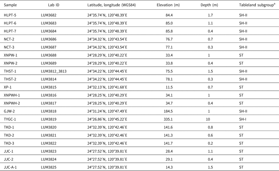
a SH-I, SH-II, Sedimentary Highlands; ST, Sedimentary Terraces.
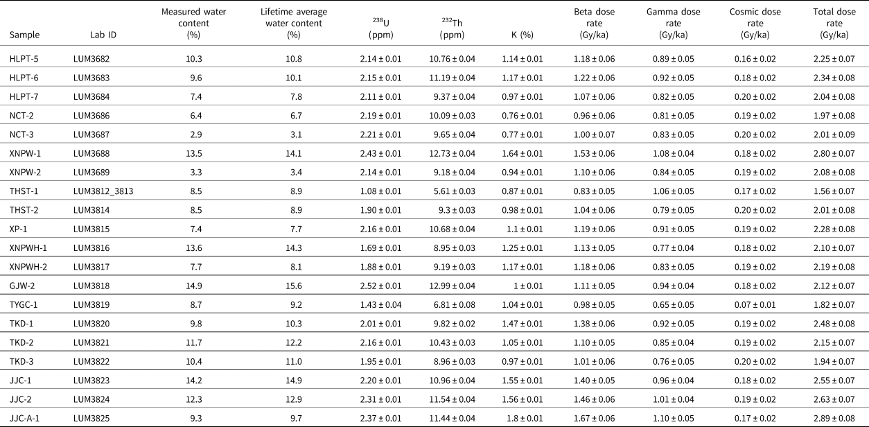
Table 3. Summary of the dosimetry measurements and calculation of total dose rates.
The outcrops were chosen in areas with respect to the different tableland subgroups (Fig. 2) to develop a chronological frame for the model of a stepwise resedimentation of the gravels and cobbles (Liu et al., Reference Liu, Hebenstreit and Böse2022). Outcrops 029_GJW and 032_THST are located in the proximal segments of SH-II; outcrop 007_NCT is located at the fringe of the biggest segment (i.e., Chiding, 崎頂) (Figs. 1b and 2a); and outcrop 001_HLPT is located at the fringe of a distal segment of the SH-II. Outcrops 025_JJC, 013_TKD, 023_XNPW, 031_XNPWH, and 015_XP are located at the fringe of the distal segments of the Sedimentary Terraces (ST).
Outcrop 030_TYGC is the only one in the southern Sedimentary Highlands (SH-I) where suitable sediments were accessible for sampling. Here, sandy deposits are exposed below 9-m-thick gravels and cobbles. However, their stratigraphic relationship with the SL layer in the SH-II and ST remains uncertain (Fig. 2a).
In addition, we used a handheld GPS receiver to record coordinates of the outcrops and extracted elevations from the high-precision open-access digital elevation model (DEM) (NASA JPL, 2013; Satellite Survey Center, 2018). Then we calculated the height of each outcrop with an uncertainty of ± 0.75 m (Satellite Survey Center, 2018). We also measured the thickness and depth below surface of each sampled deposit to calculate the elevation of the OSL sampling points. These elevation data were also used for the subsequent calculation of the uplift rates, and related uncertainties were derived from the error range of age estimations.
Sample preparation
The preparation and measurements of the quartz-OSL samples were performed between 2017 and 2018 in the luminescence laboratory at the Leibniz Institute for Applied Geophysics in Hanover, Germany. All laboratory work was done under subdued red-light conditions to prevent the grains from being bleached by artificial light sources. The sediments of both ends of the sampling cylinders were removed, because these grains were possibly bleached during the sampling. The samples were prepared by methods based on Mejdahl and Christiansen (Reference Mejdahl and Christiansen1994) for the extraction of quartz grains: (1) drying of the samples at max. 50°C for 24 h; (2) sieving to separate a suitable grain size, we used the grain-size range of 150–200 μm for the CW-OSL measurements (because all 20 samples contained sufficient amounts of this grain size, it was used for all the samples for the sake of consistency); (3) removal of carbonates by adding HCl (10%); (4) destruction of aggregates by adding sodium oxalate; and (5) removal of organic matter by adding H2O2 (30%). Heavy liquid separation was subsequently applied to separate the quartz grains from the other minerals. The quartz grains were then etched with HF solution (40%) for 60 min; this procedure dissolved the remaining feldspar grains and the outer part of quartz grains that were exposed to the alpha radiation (Mejdahl and Christiansen, Reference Mejdahl and Christiansen1994). A final sieving was carried out after the HF etching step.
Experimental setup
The quartz grains were mounted on stainless steel disks (diameter = 9 mm) and were fixed to an adhesive spot (using silicone oil) of 2 mm diameter at the center of each disk. These 2 mm aliquots each contained approximately 100 grains (Duller, Reference Duller2008). Sample NCT-2 was chosen for the evaluation of protocols and dose recovery characteristics (Fig. 3). Dose recovery tests and subsequent measurements were carried out using a Risø TL/OSL reader (model DA-20). The stimulation system was fit with blue LEDs (470 nm) for OSL stimulation and IR LEDs (870 nm) for IRSL stimulation (Bøtter-Jensen et al., Reference Bøtter-Jensen, Bulur, Duller and Murray2000, Reference Bøtter-Jensen, Thomsen and Jain2010). The luminescence signal detection units were mounted with a Hoya U-340 filter to measure the quartz-OSL signal (Bøtter-Jensen et al., Reference Bøtter-Jensen, Bulur, Duller and Murray2000, Reference Bøtter-Jensen, Thomsen and Jain2010). The test protocol included an additional stimulation step for the feldspar-IRSL signal to study the feldspar contamination of each aliquot (i.e., depletion test) (Duller, Reference Duller2003).
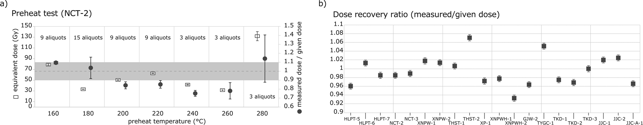
Figure 3. Preheat and dose recovery test of all samples. (a) Results of the preheat and dose recovery tests obtained from the quartz grains of the sample NCT-2; the recycling ratios and equivalent doses were tested in 20°C increments from 160°C to 300°C. (b) The dose recovery test results for all other samples have the same setting of preheat (180°C) and cut-heat temperature (160°C) as for NCT-2. These results were all obtained without a hot-bleaching procedure.
Dose recovery tests were conducted with a given dose of 63.5 Gy at preheat temperatures ranging from 180°C to 300°C (tested every 20°C) (Fig. 3). The recovered/given dose ratio showed good (0.9–1.1) results for 160°C and 180°C, but less favorable results at higher preheat temperatures. We set 180°C as the preheat temperature and 160°C as the cut-heat for the subsequent dose recovery tests conducted for all samples to validate the reproducibility of the SAR protocol. Data evaluation was carried out using rejection criteria for recycling of ±10% (Rhodes, Reference Rhodes2011) and 5% of the natural signal for recuperation (Murray and Wintle, Reference Murray and Wintle2000). The results show that all samples have a recovered/given dose ratio within the range of 0.9 to 1.1, which proves the suitability of the SAR protocol (Fig. 3).
The decay curves of the quartz-OSL signals are fast component–dominated and reach the background rapidly within the first seconds of stimulation (Bailey et al., Reference Bailey, Smith and Rhodes1997; Singarayer and Bailey, Reference Singarayer and Bailey2003; Wintle and Murray, Reference Wintle and Murray2006; Durcan and Duller, Reference Durcan and Duller2011). We observed fast component–dominated natural signals for all of the accepted aliquots (Fig. 4). We followed the early background subtraction approach of Cunningham and Wallinga (Reference Cunningham and Wallinga2010) to set the time intervals for the initial signal (0–0.5 s) and background (0.6–1.5 s) to rule out any influence of medium or slow components on the net signals (Fig. 4). Most of the aliquots show very low recuperation values (<5% of the natural signal), thus the recuperation-caused underestimation of D e is negligible (Aitken and Smith, Reference Aitken and Smith1988; Supplementary Appendix B). The IR depletion was carefully checked for all aliquots (Duller, Reference Duller2003), and as expected from the results of previous studies, feldspar contamination was also identified in our samples. To test whether the feldspar contamination detected significantly affected the determined doses, we tested all samples and all measured aliquots for a potential correlation between D e and the IR-depletion ratio (Supplementary Appendix B) (based on the approach of Schmidt et al. [Reference Schmidt, Tsukamoto, Salomon, Frechen and Hetzel2012]), but although an IR contribution was detected in some aliquots, there is no significant correlation to the D e (R 2 < 0.36) for all samples; thus there is no clear relationship overall between D e and feldspar contamination (Supplementary Appendix B). This is corroborated by average IR depletion ratios close to 1 for all samples.
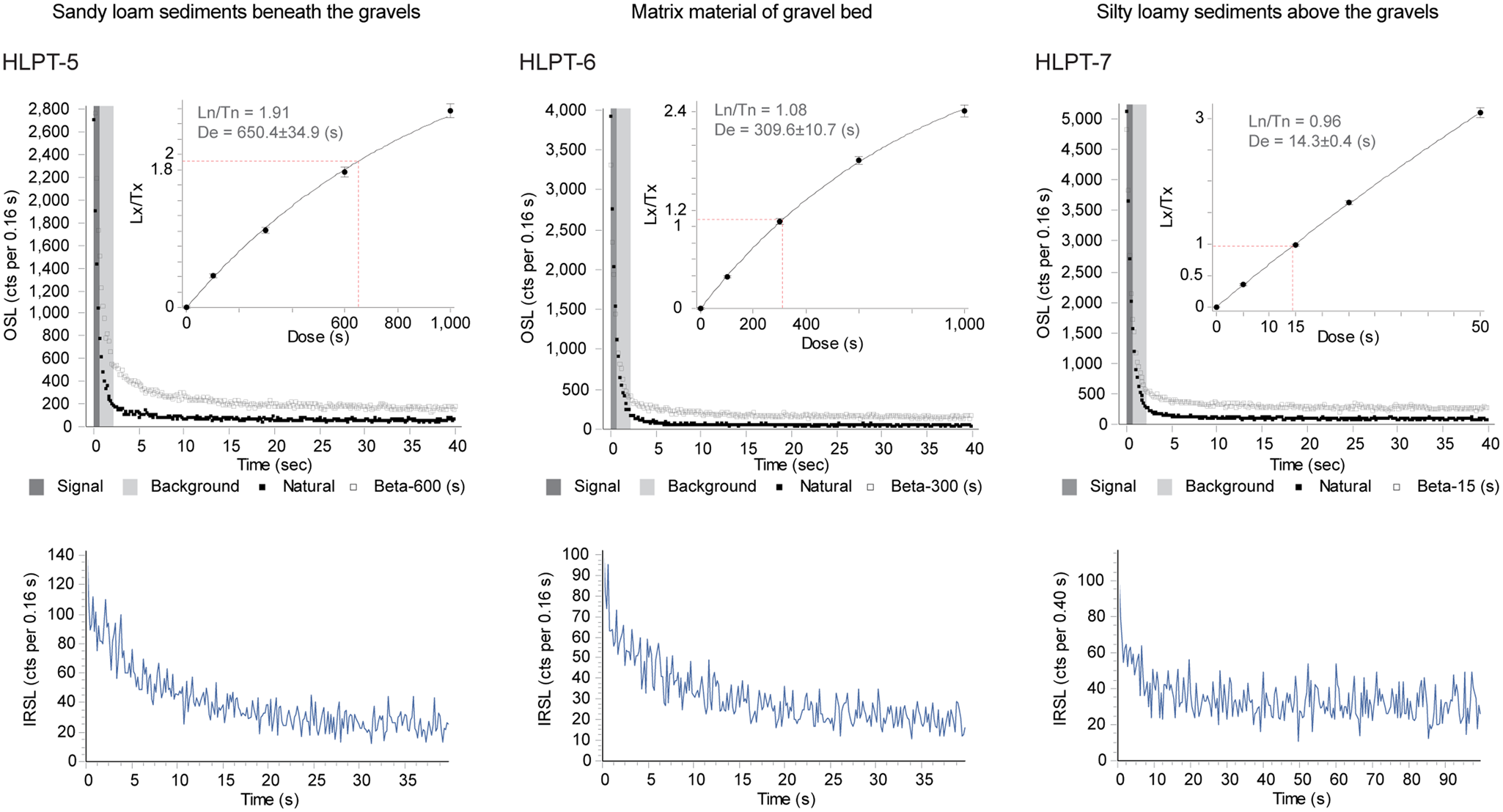
Figure 4. Representative quartz–optically simulated luminescence (OSL) decay curves, single-aliquot regenerative (SAR) growth curves, and feldspar-IRSL signals for samples within and below the gravel and cobble layer (CSB) (see Supplementary Appendix B for the detailed results of all samples). The fast component is clearly dominant; the feldspar-IRSL signals are relatively weak and only contribute to the background noise.
Measurements of equivalent dose and dose rate
For each sample, D e measurements were performed on at least 40 aliquots (XP-1 and JJC-1). For the majority of the samples, we measured around 42 to 84 aliquots, the maximum amount being 102 aliquots for sample NCT-2 (Table 4). Thus, we collected at least 24 or more aliquots of each sample for the D e determination, as recommended in relevant studies (Galbraith and Roberts, Reference Galbraith and Roberts2012; Rixhon et al., Reference Rixhon, Briant, Cordier, Duval, Jones and Scholz2017). The rejection criteria of the recycling ratio and the recuperation ratio were based on the aforementioned tests. In addition, the 2D 0 test was applied to check whether aliquots were in field saturation (Wintle and Murray, Reference Wintle and Murray2006).
Table 4. Results of quartz–optically simulated luminescence (OSL) dating and age estimations.a
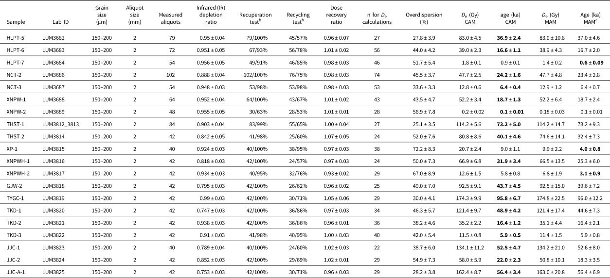
a CAM, central age model; MAM, minimum age model.
b The majority of ages are based on the CAM data, except for three samples which are based on the MAM data (Sigma b = 0.45) due to the incomplete bleaching effects.
c The MAM ages used in the interpretations are marked in bold.
For the determination of the environmental dose rate, the sediments were dried at 75°C for more than 24 h to measure their water content (%), and then the sediments were homogenized with a mortar and pestle to break the aggregates of fine-grained sediments and sealed (about 700 g) in a Marinelli beaker for more than 6 weeks to achieve equilibrium between 222Rn and 226Ra (Aitken, Reference Aitken1985; Guérin et al., Reference Guérin, Mercier and Adamiec2011). The content of naturally occurring radionuclides (decay chains of 235U and 232Th, as well as 40K) was determined by measurements using high-resolution, low-level gamma spectrometry (high-purity p-type germanium detector). The gamma efficiency calibrations were performed by using the reference materials RGK-1, RGU-1, and RTh-1 from IAEA with either 50 or 700 g (depending on the sample amount). The determined radionuclide contents were then included in dose rate calculations using the conversion factors provided by Guérin et al. (Reference Guérin, Mercier and Adamiec2011; Table 3).
Equivalent dose determination and dose-rate and age calculations
We exported the original measured data (e.g., D e and error of each aliquot) from the Risø-Analyst software (Bøtter-Jensen et al., Reference Bøtter-Jensen, Bulur, Duller and Murray2000) and implemented the age model calculations with the R-luminescence package in R Studio (Kreutzer et al., Reference Kreutzer, Schmidt, Fuchs, Dietze, Fischer and Fuchs2012). We first used the central age model (CAM) (Galbraith et al., Reference Galbraith, Roberts, Laslett, Yoshida and Olley1999) to calculate the central dose for all the samples, as well as to determine the corresponding overdispersions (OD) (Galbraith et al., Reference Galbraith, Roberts, Laslett, Yoshida and Olley1999). Kernel density estimate (KDE) plots were generated for the D e distributions of all samples using the R-luminescence package (Kreutzer et al., Reference Kreutzer, Schmidt, Fuchs, Dietze, Fischer and Fuchs2012).
The acceptance rates of the recuperation test were 91% to 100% for most samples, except for sample XNPW-2 (Table 4), which showed higher recuperation values and only 30 of 48 aliquots (ca. 63%) were accepted following the recuperation test (Table 4). The acceptance rates of the recycling test range from 53% to 98%, and two groups can be differentiated. The group with the higher acceptance ratio (85 to 98%) consists of samples mostly taken from the SiL layers; only two are taken from the CSB layer (TKD-2) and the SL layer (TKD-1) (Table 4). The group of samples with the lower acceptance rate (53% to 78%) are mainly derived from the SL layer. The worst acceptance rate concerning the recycling test (53%) was again observed for sample XNPW-2 (Table 4).
As a result of the additional 2D 0 test for saturation of the quartz grains, only 13 aliquots in total had to be rejected for the subsequent D e determination (Wintle and Murray, Reference Wintle and Murray2006). They occurred in nine samples (two for HLPT-5, two for NCT-2, one for THST-1, one for THST-2, one for GJW-2, one for TYGC-1, two for TKD-1, two for JJC-1, and one for JJC-A-1).
The skewness of the D e distributions ranges between −0.42 and 2.59 (Table 4); two samples are slightly left skewed (THST-1 and GJW-2), all other D e distributions are right skewed (from 0.08 to 2.59). The highly right-skewed samples are XNPWH-2 (2.59), JJC-2 (1.73), XNPW-2 (1.73), TKD-3 (1.5), NCT-3 (1.42), JJC-A-1 (1.42), HLPT-7 (1.3), and XP-1 (1.17), half of these highly right-skewed samples are taken from the SiL layer. The OD values for all samples range between 27.8 ± 3.9% and 72.2 ± 8.3% (Table 4). The samples with higher OD values (>45%) are mostly taken from the SiL layer, except samples XNWPH-1 (50.0 ± 7.3%) and TKD-1 (46.3 ± 5.7%). While some samples show rather broad, but symmetrical dose distributions, the majority show multimodal or right-skewed distributions (Fig. 5). The corresponding OD values for the samples showing rather symmetrical distributions average about 45%. These are the samples we expect to represent the minimal overdispersion to be achieved in nature for well-bleached samples from the research area. These multimodal or right-skewed dose distributions may indicate incomplete bleaching prior to burial to be significant for these samples (Stokes et al., Reference Stokes, Bray and Blum2001). Thus, the residual doses remain, causing a shift toward higher D e values (Jain et al., Reference Jain, Murray and Botter-Jensen2004). For example, long-lasting or long-distance reworking processes yield a higher bleaching probability than rapid and short-distance (e.g., flooding) reworking processes (Arnold and Roberts, Reference Arnold and Roberts2009; Gray and Mahan, Reference Gray and Mahan2015).
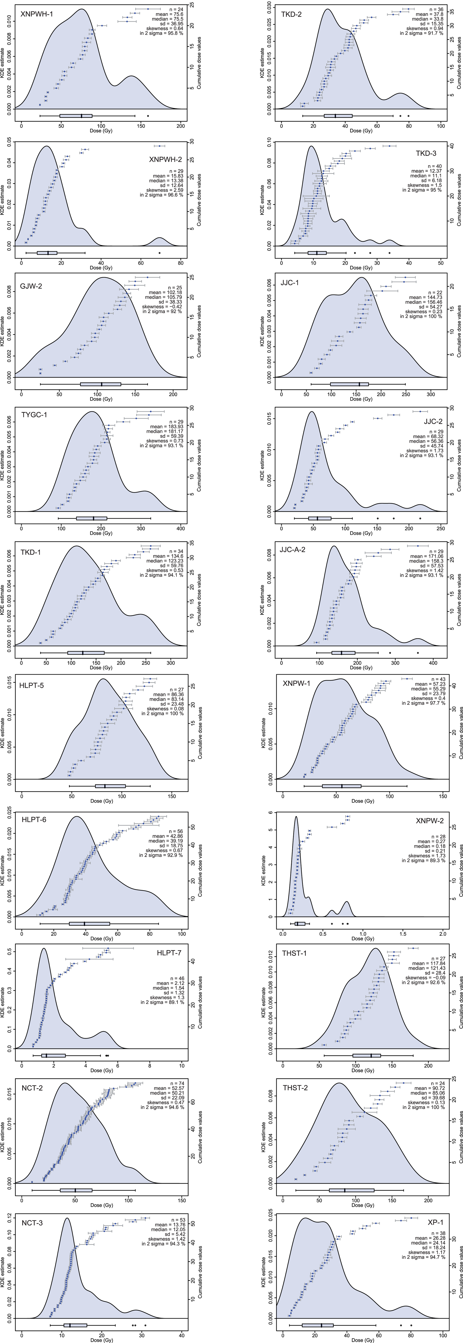
Figure 5. The kernel density estimate (KDE) plots for the D e distribution of all optically simulated luminescence (OSL) samples. All samples of coastal fine-grained sediments and the matrix sediments of the gravel and cobble layer present symmetrical but relatively broad D e distributions. Three samples from the uppermost layer (HLPT-7, XP-1, and XNPWH-2), however, present highly right-skewed D e distributions with some isolated higher data point(s). The high overdispersion values are interpreted to result from incomplete bleaching. To address incomplete bleaching effects, the minimum age model (MAM) was applied to these three samples, and central age model (CAM) ages were used for the other samples.
To address the effects of incomplete bleaching in the calculation of the D e values, we used the three-parameter minimum age model (MAM) (Galbraith et al., Reference Galbraith, Roberts, Laslett, Yoshida and Olley1999) with sigmab = 0.45 as determined to be the average scatter for symmetrical dose distributions, for all samples. The results showed the CAM- and MAM-based ages agreed within error for the large majority of samples, except for three samples: HLPT-7, XP-1, and XNPWH-2 (Table. 4). We therefore concluded that incomplete bleaching significantly affected these samples and used the MAM-based (with sigmab = 0.45) D e values for subsequent age calculation; the CAM-based D e values were used for age calculation of all other samples. The corresponding ages used for all later interpretation are marked in bold in Table 4.
The dose rate calculations were based on the function comprising dose rate conversion parameters (Rees-Jones, Reference Rees-Jones1995; Guérin et al., Reference Guérin, Mercier and Adamiec2011) as well as the water content, the beta-dose attenuation (Aitken, Reference Aitken1985; Adamiec and Aitken, Reference Adamiec and Aitken1998), and the cosmic-dose attenuation (Prescott and Stephan, Reference Prescott and Stephan1982; Prescott and Hutton, Reference Prescott and Hutton1994). Due to the loss of moisture since the excavation of the sampled outcrops, we estimated the lifetime water content for each sample by adding 5% to the measured water content. The 5% additional water content contributed to a broader error range of the dose rate for ±0.04–0.05 Gy/ka (ca. 2% wider). The depositional ages were calculated with the empirical calculation of the D e and the dose rate using a spreadsheet (Table 4).
RESULTS
All luminescence samples showed robust results in the pretests, and the SAR protocol we chose yielded accurate D e estimates for the samples under investigation. Although feldspar contamination was detected for some aliquots, this did not have a systematic effect on the equivalent dose. Sample TYGC-1 showed rather high equivalent doses, with the dose–response curve approaching saturation in that dose range. The resulting age must therefore be handled with care, as it may actually represent a minimum age (Table 4, Supplementary Appendix C). Using the average of scatter expressed as the overdispersion (OD or sigmab) for the well-bleached samples’ (symmetrical) dose distributions as a threshold value, it was possible to identify those samples from the data set that were significantly affected by incomplete bleaching (HLPT-7, XP-1, and XNPWH-2). These three samples showed right-skewed D e distributions, including some very high data point(s) (Fig. 5, Table 4), and were also characterized by high OD values. To account for the effects of incomplete bleaching, we used the MAM-based D e values for the age calculation of these three samples, with CAM ages adopted for all other samples (Fig. 5, Table 4). Although the quartz luminescence properties we encountered in this study are not ideal, we carefully investigated the potential influence of feldspar contamination and did not observe any dose dependence with regard to the IR depletion ratio. Average IR depletion ratios for all samples were observed to be close to 1. In addition, all samples showed excellent results in dose recovery experiments. Only one sample was approaching signal saturation. We therefore consider our luminescence analyses to provide reliable depositional ages.
The total dose rate ranges from 1.51 ± 0.07 Gy/ka (THST-1) as the minimum and 2.89 ± 0.08 Gy/ka (JJC-A-1) among the 20 studied OSL samples (Table 3). The differences in the cosmic dose contribution among the samples are insignificant, as they only contributed 0.07 ± 0.01 mGy/ka (TYGC-1) to 0.20 ± 0.02 mGy/ka (HLPT-7; THST-2; TKD-3). The beta dose rates are more diverse. They differ from site to site, which is more significant than the difference among the different sedimentary layers in the same site (Table 3). The sites in the distal segments contain higher concentration of radioactive nuclides, and vice versa.
The overall depositional ages of the upper part of sedimentary successions in the Miaoli Tableland from the obtained OSL measurements range from ca. 95.7 ± 6.7 ka (TYGC-1, LUM3819) to ca. 0.1 ± 0.01 ka (XNPW-2, LUM3689).
The results can be categorized tentatively from the post–last interglacial to the Holocene (Figs. 2 and 6, Table 4):
1. post–last interglacial sandy deposits in the SH-I (TYGC-1), n = 1;
2. MIS 4 sandy deposits in the proximal segments of the SH-II (THST-1), n = 1;
3. MIS 3 to 2 sandy deposits in the distal segments of the SH-II (HLPT-5) and the ST (XNPW-1, XNPWH-1, TKD-1, JJC-1, JJC-A-1), n = 6;
4. MIS 3 silty cover layers in the proximal SH-II segments (THST-2, GJW-2), n = 2;
5. MIS 2 silty cover layers in the distal segments of the SH-II (NCT-2) and sandy deposits in the ST (JJC-2), n = 2;
6. MIS 2 gravel and cobble layer(s) of the SH-II (HLPT-6) and ST (TKD-2), n = 2;
7. Holocene silty cover layers in the distal segments of the SH-II (HLPT-7, NCT-3) and ST (XNPW-2, XNPWH-2, XP-1, TKD-3), n = 6.

Figure 6. Comparison of the optically simulated luminescence (OSL) ages of the studied sedimentary succession compared with the paleoclimate record after Liew et al. (Reference Liew, Huang and Kuo2006). The Marine Oxygen Isotope Stages (MIS) were simplified from the global δ 18O curve of Lisiecki and Raymo (Reference Lisiecki and Raymo2005) and Cohen et al. (Reference Cohen, Harper and Gibbard2020). The OSL samples are plotted by the age with uncertainties (x-axis) and relative elevations in the classification of each layer (y-axis). The ages of each outcrop are graphically connected by the colored lines and shadings according to their corresponding tableland segment subcategories (Sedimentary Highlands in the southeast [SH-I], dark gray; in the north and northwest [SH-II], magenta; Sedimentary Terraces [ST], cyan); thus the depositional age of the gravels and cobbles can be tentatively marked with the corresponding intervals by bracketing the ages of the sandy loam (SL) layer (upper limit) and the silty loam layer (SiL) layer (lower limit).
DISCUSSION
OSL ages of the sedimentary units
The numerical ages of the post–last interglacial to modern depositions are presented in stratigraphic order in the respective outcrops (Fig. 2). They generally match the late Pleistocene age estimation of Chang et al. (Reference Chang, Teng and Liu1998) and the radiocarbon dates of mollusks in coastal sediments (sandy deposits) in the distal part of the tableland falling into MIS 3 (Wang and Peng, Reference Wang and Peng1990). Furthermore, our results allow a more detailed chronological framework for the deposition of the coastal and fluvial sediments in the upper layers in the Miaoli Tableland, which agrees with the assumption that the beginning of the deposition of the lower part of the sediment succession occurred during the middle Pleistocene (Ota et al., Reference Ota, Lin, Chen, Chang and Hung2006).
Age of the sandy loam layer (SL)
The SL layer is distributed over the entire area of the Miaoli Tableland. Liu et al. (Reference Liu, Hebenstreit and Böse2022) interpret these sediments as a near-coast (beach) sandy accumulation in the foreland of the WF. The age estimation of sample TYGC-1 in the SH-I was affected by saturation of the quartz grains, even though most of the aliquots passed the 2D 0 test. Therefore, we took this age estimation (95.7 ± 6.7 ka, TYGC-1) as a minimum age rather than a real depositional age, and we assume the real depositional age for this sandy loamy substrate should be earlier than 100 ka. In this context, we interpret the sampled coastal (beach) sediments as representing the beginning of a post–last interglacial sea-level lowering (Figs. 2a and 6), which resulted in regression in the shallow terrain of the Taiwan Strait (Liu et al., Reference Liu, Xia, Berne, Wang, Marsset, Tang and Bourillet1998; Jan et al., Reference Jan, Wang, Chern and Chao2002; Liu et al., Reference Liu, Liu, Xu, Milliman, Chiu, Kao and Lin2008).
The age estimation of the SL layer in the proximal segments of the SH-II in outcrop 032_THST (deposited at 73.1 ± 5.0 ka, THST-1) can be related to a further regression at the cold phase that began during the early MIS 4 (Waelbroeck et al., Reference Waelbroeck, Labeyrie, Michel, Duplessy, McManus, Lambeck, Balbon and Labracherie2002) (Figs. 2b and 7b).
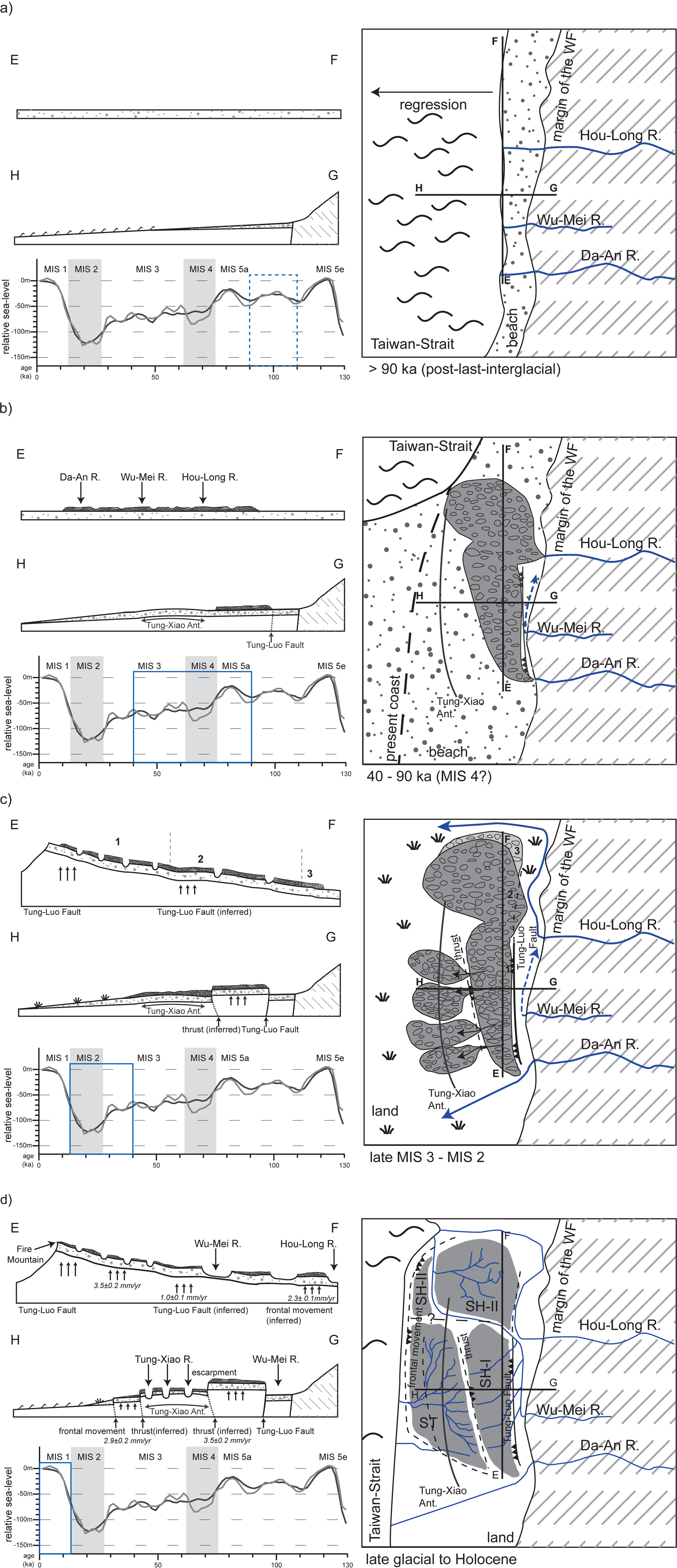
Figure 7. Schematic sketch of a morphological landscape evolution model of the Miaoli Tableland in four time steps (a, b, c, and d). Each step shows a south–north (E–F) and east–west (G–H) profile, a sketch map, and the global sea-level curve simplified from Waelbroeck et al. (Reference Waelbroeck, Labeyrie, Michel, Duplessy, McManus, Lambeck, Balbon and Labracherie2002) with the mark of the respective period. The location of the coastlines are referenced from Fig. 1a; the tectonic features after Shyu et al. (Reference Shyu, Sieh, Chen and Liu2005), Ota et al. (Reference Ota, Lin, Chen, Chang and Hung2006), and Yang et al. (Reference Yang, Rau, Chang, Hsieh, Ting, Huang, Wu and Tang2016). For a detailed description see “Landform Evolution Model.” MIS, Marine Oxygen Isotope Stage; SH-I, SH-II, Sedimentary Highlands; ST, Sedimentary Terraces; WF, Western Foothills.
Another group of ages is represented by outcrops 013_TKD (48.9 ± 4.2 ka, TKD-1) and 025_JJC (56.3 ± 3.4 ka, JJC-A-1; 52.5 ± 4.7 ka, JJC-1) (Figs. 2b and 6). The remarkable westward inclination of the SL layer (Liu et al., Reference Liu, Böse and Hebenstreit2021) in outcrop 025_JJC (Supplementary Appendix A) is mainly influenced by the Tung-Xiao Anticline (Yang et al., Reference Yang, Huang, Wu, Ting and Mei2006, Reference Yang, Rau, Chang, Hsieh, Ting, Huang, Wu and Tang2016; Figs. 1b and c and 2) and took place after the deposition of the coastal sediments. In contrast, the SL layers of the 023_XNPW and 031_XNPWH outcrops in the immediate vicinity do not show any inclination and were presumably deposited after the tectonic displacement according to their younger ages (31.9 ± 3.4 ka, XNPWH-1; 18.7 ± 1.3 ka, XNPW-1). This also indicates that the anticline was active during a time span around 50–30 ka.
The age in the northern SH-II segments (36.9 ± 2.4 ka, HLPT-5) falls between the aforementioned groups. Overall, the ages of the SL layer indicate that the deposition of coastal (beach) sediments took place over a long period of time during the late MIS 5 to MIS 2 in the area of today's Miaoli Tableland, and the ages are generally getting younger north- and westward (Figs. 2 and 6), implying that the coastline moved northwestward during the last glacial period, which is in agreement with the regression in the Taiwan Strait (Jan et al., Reference Jan, Wang, Chern and Chao2002). However, local postdepositional remobilization of the highly mobile sand may explain the relatively young age of 18.7 ± 1.3 ka (XNPW-1).
Age of the cover layers (SiL)
Eolian sediments cover large parts of the Miaoli Tableland (Liu et al., Reference Liu, Hebenstreit and Böse2022); our respective OSL ages range from 43.7 ± 4.5 ka (GJW-2) to 0.1 ± 0.1 ka (XNPWH-2). The depositional ages are consistent in outcrop 029_GJW (43.7 ± 4.5 ka, GJW-2) and outcrop 032_THST (40.1 ± 4.6 ka, THST-2). These samples represent the oldest eolian accumulations in the area, found on the large proximal segments in the SH-II, deposited during MIS 3. In two outcrops in the SH-II and the ST, the sampled eolian sediments were deposited during MIS 2 (24.2 ± 1.6 ka, NCT-2; 22.0 ± 2.3 ka, JJC-2), respectively. The youngest eolian sediments began being deposited on both the distal segments of the SH-II (0.6 ± 0.1 ka, HLPT-7; 6.4 ± 0.4 ka, NCT-3) and the ST (0.1 ± 0.1 ka, XNPW-2; 5.8 ± 0.7 ka, XNPWH-2; 9.1 ± 1.1 ka, XP-1; 5.9 ± 0.5 ka, TKD-3) during the Holocene and continued being deposited until the present day (Fig. 7d, Table 4).
These ages correlate well with the degree of the in situ weathering and pedogenesis in the studied outcrops, which affect the upper sediment layers on the tableland surfaces (Tsai et al., Reference Tsai, Hseu, Huang, Huang and Chen2010). We derived the oldest ages from the larger (better-preserved) tableland segments, where the color of the surface substrate appeared to be reddish-ocher (see “Introduction”). Assuming a more or less continuous dust deposition over the study area during the last glacial cycle, the age distribution of the cover layer samples represents the preservation status of the tableland segments.
Similar cover layers or soils with eolian dust input have also been recognized and described in a variety of geomorphological settings and at all altitudes in Taiwan (Hebenstreit, Reference Hebenstreit2016; Tsai et al., Reference Tsai, Chen, Huang, Huang, Hseu and You2021), for example, in the Dadu Tableland and the Puli Tableland (Tsai et al., Reference Tsai, Hseu, Huang, Huang and Chen2010; Tseng et al., Reference Tseng, Lüthgens, Tsukamoto, Reimann, Frechen and Böse2016), as well as in the mountain ranges, where the ages range from 0.7 ka in the Nanhua Shan (Tsai et al., Reference Tsai, Chen, Huang, Huang, Hseu and You2021) to ca. 3–4 ka in the Nanhuta Shan and Hehuan Shan (Hebenstreit et al. Reference Hebenstreit, Böse and Murray2006, Wenske et al., Reference Wenske, Böse, Frechen and Lüthgens2011), and 54.8 ka in the Tachia River catchment (Wenske et al., Reference Wenske, Frechen, Böse, Reimann, Tseng and Hoelzmann2012).
The eolian sediments originate from a mixture of dust brought mainly from the Asian continent (Pye and Zhou, Reference Pye and Zhou1989; Chen et al., Reference Chen, Yeh, Song, Hsu, Yang, Wang and Chi2013) until the present (Lin et al., Reference Lin, Wang, Chen, Chang, Chou, Sugimoto and Zhao2007; Hsu et al., Reference Hsu, Liu, Arimoto, Liu, Huang, Tsai, Lin and Kao2009) and locally reworked fine-grained sediments (Tsai et al., Reference Tsai, Huang, Hseu and Chen2006, Reference Tsai, Maejima and Hseu2008, Reference Tsai, Hseu, Huang, Huang and Chen2010, Reference Tsai, Chen, Huang, Huang, Hseu and You2021; Wenske et al., Reference Wenske, Frechen, Böse, Reimann, Tseng and Hoelzmann2012).
Age of the gravel and cobble layers (CSB)
Direct dating results from the gravel and cobble depositions (CSB) are only available for two samples in the SH-II (16.4 ± 1.2 ka, HLPT-6) and ST (16.6 ± 1.1 ka, TKD-2). Therefore, we used bracketing ages from the upper and lower boundary layers to estimate the ages of more CSB layers (Fig. 6).
As the underlying coastal sediments at outcrop 030_TYGC (sample TYGC-1) yielded an age that has to be interpreted as a minimum age >95.8 ± 6.7 ka, we conclude that the deposition of the thick gravels and cobbles of the SH-I is younger than this age. This agrees with Ota et al. (Reference Ota, Lin, Chen, Chang and Hung2006), who assume an age older than 90 ka based on the degree of surface weathering of the “Sanyi Tableland” (SH-I). On the other hand, the gravels and cobbles on the proximal segments of the SH-II were deposited before ca. 40 ka, as estimated from the age of the overlying cover layer at outcrops 032_THST and 029_GJW (Figs. 2a and 6). The gravels and cobbles in the Sedimentary Highlands can therefore be related to an early stage of the last glacial cycle, probably to the MIS 4 cold phase (see “Landform Evolution Model”).
The depositional age of the gravels and cobbles in the Sedimentary Terrace (ST) area can be estimated from the under- and overlying layers at the three outcrops 025_JJC, 023_XNPW, and 031_XNPWH, beside the direct age (16.6 ± 1.1 ka, TKD-2). The abovementioned inclination of the subjacent coastal sands (SL layer) at outcrop 025_JJC has affected neither the overlying gravels and cobbles nor the neighboring coastal sands at outcrops 023_XNPW and 031_XNPWH. We can infer that the gravel accumulation in the ST began not earlier than the end of the activity of the Tung-Xiao Anticline at about 30 ka, as indicated by its age in the outcrop XNPWH (31.8 ± 3.4 ka, XNPWH-1). However, in 023_XNPW, the gravels and cobbles must be even younger than the underlying sands (18.6 ± 1.3 ka, XNPW-1). The directly dated gravels and cobbles at outcrop 013_TKD in the northwestern ST confirm this time period. On the other hand, the cover layer at 025_JJC implies an earlier deposition of the gravels and cobbles already before (22.0 ± 2.3 ka, JJC-2) at this location. From our data, we assume a general time frame for the deposition of the ST gravels and cobbles during the MIS 2 cold phase (see “Landform Evolution Model”). However, the special and temporal resolution is not high enough to distinguish between individual gravel and cobble accumulation events.
Uplift rates of the Miaoli area
The Miaoli Tableland does not represent fluvial terraces in a strict sense, although the upper sedimentary units are composed of fluvial gravels and cobbles and the tableland is dissected by fluvial incision. However, the underlying sediment units represent a sequence of coastal and, in the deeper part, shallow-marine (tidal) sediments (Lin, Reference Lin1963; Liu et al., Reference Liu, Hebenstreit and Böse2022). To infer estimates of uplift rates in the area, we calculated the vertical displacement by using the uppermost parts of the coastal sediment (SL layer). A similar approach was taken in southern Taiwan (Chen and Liu, Reference Chen and Liu2000) and Japan (Matstu'ura et al. Reference Matsu'ura, Kimura, Komatsubara, Goto, Yanagida, Ichikawa and Furusawa2014), and by Ota and Yamaguchi (Reference Ota and Yamaguchi2004) with examples from the western Pacific area. Assuming that the coastline in the Taiwan Strait was lower than today at the time of deposition and taking the present coastline as a benchmark, the resulting uplift rates represent minimum values for each outcrop.
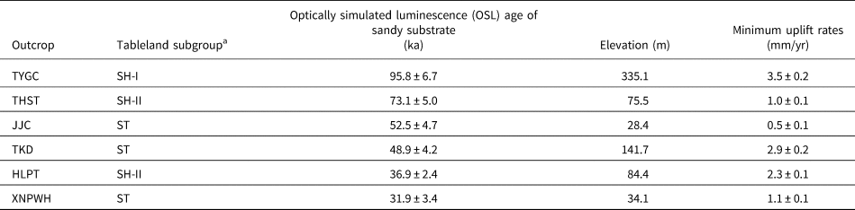
The calculations resulted in spatially heterogeneous uplift rates (Fig. 7c and d, Table 5) in the Miaoli Tableland. In the Sedimentary Highlands the highest rate is found at outcrop 030_TYGC with 3.5 ± 0.2 mm/yr, reflecting a relatively rapid uplift of the SH-I in the last ca. 100 ka, which is mainly controlled by the Tung-Luo Fault (Fig. 1) in the east (Ota et al., Reference Ota, Lin, Chen, Chang and Hung2006). In the SH-II, the uplift rates are 2.3 ± 0.1 mm/yr at outcrop 001_HLPT and only ca. 1 ± 0.1 mm/yr at outcrop 032_THST.
Table 5. Calculation of the uplift rates.
a SH-I, SH-II, Sedimentary Highlands; ST, Sedimentary Terraces.
The uplift rates in the ST area are rather low in the southwestern part. The uplift of 28 and 34 m in the 025_JJC and the 031_XNPWH, respectively, results in an average rate of 0.5–1.1 mm/yr since MIS 2/3. In contrast, the coastal sediments in the outcrop 013_TKD imply an uplift of ca. 142 m in ca. 49 ka at a rate of 2.9 mm/yr, which might be due to the vicinity of the frontal movement at the coastal area (Shyu et al., Reference Shyu, Sieh, Chen and Liu2005; Yang et al., Reference Yang, Rau, Chang, Hsieh, Ting, Huang, Wu and Tang2016).
Our calculated uplift rates are comparable with the previously estimated average of 2 mm/yr for the last 45–30 ka in the Miaoli Tableland (Wang and Peng, Reference Wang and Peng1990), but relatively low compared with rates farther south in the western Taiwan mountain foreland, where Holocene uplift rates of beach and marine sediments of 5–7 mm/yr and 7.7–4.3 ka, respectively, are reported from the Tainan area (Chen and Liu, Reference Chen and Liu2000; Hsieh and Knuepfer, Reference Hsieh and Knuepfer2001).
The tectonic influence on the morphodynamics in the western Taiwan tablelands is interpreted as a partitioned model (Siame et al., Reference Siame, Chen, Derrieux, Lee, Chang, Bourlès, Braucher, Léanni, Kang, Chang and Chu2012); major tectonic events, rather than continuous processes, might cause the main offsets. For example, the Chi-Chi earthquake in 1999 caused ca. 10 m of vertical offset of the Chelunpu Thrust Fault in the nearby Shi-Gang (ca. 12 km southeast) and Feng-Yuan areas (ca. 17 km south) (Chen et al., Reference Chen, Chen, Chen, Zhang, Zhao, Zhou and Li2003a; Yue et al., Reference Yue, Suppe and Hung2005; Fig. 1a).
Landform evolution model
Combining our results and interpretations, we propose a landform evolution model, integrating the results from Chang et al. (Reference Chang, Teng and Liu1998), Ota et al. (Reference Ota, Lin, Chen, Chang and Hung2006), and Liu et al. (Reference Liu, Hebenstreit and Böse2022), of the Miaoli Tableland in four time slices as follows (Figs. 1b and 7):
1. The lowering of the sea level after the high stand of the last interglacial caused a regression in the western mountain foreland. The upper coastal sediments of the foreland basin in today's SH-I area were accumulated at that time. The deposition of the beach sediments follows the ongoing northwestward shoreline progradation (Fig. 7a).
2. During the following cold phase (MIS 4 and probably until the beginning of MIS 3), the sea-level lowering shifted the base level to a lower level and farther away from the mountain front. Cold and wet climate conditions are documented by a vegetation change in the mid-altitude area (1000–3000 m asl) in the mountain ranges (Liew et al., Reference Liew, Huang and Kuo2006; Fig. 6). Glacial and periglacial conditions prevailed in the upper mountain ranges at that time (Hebenstreit et al., Reference Hebenstreit, Böse and Murray2006, Reference Hebenstreit, Ivy-Ochs, Kubik, Schlüchter and Böse2011; Klose, Reference Klose2006), which resulted in a higher yield of coarse clasts in the rivers. The rivers transported gravels and cobbles from the mountain ranges and the WF into the newly emerged foreland area. They were deposited as alluvial fans that formed the thick gravel and cobble bed of the later Sedimentary Highlands (SH-I and SH-II) (Ota et al., Reference Ota, Lin, Chen, Chang and Hung2006; Liu et al., Reference Liu, Hebenstreit and Böse2022; Figs. 6 and 7b). These gravels and cobbles were previously interpreted as deposits from multiple sources, such as the Da-An River for the south of the SH-I and the Hou-Long River for the north of the SH-I and the proximal area of the SH-II (Chang et al., Reference Chang, Teng and Liu1998; Fig. 1b). We follow this assumption. However, due to the similar lithology in the catchments of the rivers that drain the WF and the mountain ranges, it is difficult to distinguish the origin of gravels and cobbles based on physical properties such as composition, shape, or roundness (Liu et al., Reference Liu, Böse and Hebenstreit2021, Reference Liu, Hebenstreit and Böse2022).
Initial uplift took place along the Tung-Luo Fault just after the deposition of the gravels and cobbles, which resulted in a first incision of the Sedimentary Highlands, followed by the activity of the Tung-Xiao Anticline (Fig. 7b).
Eolian sediments subsequently covered the alluvial fans. They have been preserved in the proximal parts of the fans until today; this is also documented in their high degree of weathering. This implies that the larger segments of the present tableland surface are stable and not affected by erosion so far.
3. According to bathymetry (Jan et al., Reference Jan, Wang, Chern and Chao2002) and current sea-level models (Waelbroeck et al., Reference Waelbroeck, Labeyrie, Michel, Duplessy, McManus, Lambeck, Balbon and Labracherie2002), the Taiwan Strait was dry and the Miaoli Tableland was far from the paleocoastline (1a and 7c) from MIS 3 to 2.
The ongoing thrusting of the Tung-Luo Fault (Ota et al., Reference Ota, Lin, Chen, Chang and Hung2006) forced the Da-An River to change its fluvial path farther south, which resulted in a cut off of the gravels and cobbles yielded to the paleo-alluvial fan in the present SH-I area. This process tilted the SH-I gravels and induced runoff to the west, which resulted in a deep incision of the SH-I segments, visible in the parallel fluvial pattern (Liu et al., Reference Liu, Hebenstreit and Böse2022; Fig. 1b). The eroded gravels and cobbles were transported (reworked) to the west, forming secondary fans in the foreland, the present ST area (Fig. 7c). At the same time, the uplift in the northern alluvial fan (the present SH-II) caused initial incision and a relocation of gravels and cobbles (Liu et al., Reference Liu, Hebenstreit and Böse2022), which extended the fan to the north (Fig. 7c).
The erodibility of the sediments may have been favored by the cold climatic conditions and the sparse savannah vegetation in the mountain foreland during MIS 2 (Liew et al., Reference Liew, Huang and Kuo2006). The subsequent increase of precipitation during the late glacial (end of MIS 2) caused accelerated transport of the fluvial gravels and cobbles into the ST area. Reinforced fluvial activity at that time is documented in other locations in Taiwan as well, for example, in the intramountainous basin in Puli (Chen and Liu, Reference Chen and Liu1991; Tseng et al., Reference Tseng, Wenske, Böse, Reimann, Lüthgens and Frechen2013, Reference Tseng, Lüthgens, Tsukamoto, Reimann, Frechen and Böse2016).
Finally, the rapid uplift at the inferred thrust (Chang et al., Reference Chang, Teng and Liu1998) at the topographic divide between the SH-I and the ST beheaded the valleys in the SH-I and reversed their flow direction from west to east (Ota et al., Reference Ota, Lin, Chen, Chang and Hung2006). This therefore stopped the sediment yield toward the alluvial fans in the ST, where ongoing fluvial incision caused dissection of the topographic surfaces into tableland segments.
4. During the late glacial and the Holocene, sea level was rising rapidly. However, the whole Miaoli Tableland area, including its distal parts, was further uplifted, due to the ongoing frontal movement (Shyu et al., Reference Shyu, Sieh, Chen and Liu2005; Fig. 7d). This uplift increased the fluvial incision, which led to the intense dissection of the ST tableland segments forming a dendritic fluvial pattern (Liu et al., Reference Liu, Hebenstreit and Böse2022) and subsequently caused the deposition of secondarily reworked gravels and cobbles in the present fluvial channels and at the coastal plains (AL) (Fig. 7d).
CONCLUSION
We present detailed and reliable chronological control for the formation of the Miaoli Tableland based on luminescence dating (quartz OSL). The new chronology and the new calculation of long-term uplift rates allow distinguishing between several depositional stages of the coastal, fluvial, and eolian sediments as well as phases of erosion since the last interglacial. They provide a chronological frame for a new landform evolution model proposed by Liu et al. (Reference Liu, Hebenstreit and Böse2022), which describes a stepwise deposition and reworking of fluvial gravels and cobbles during the last glacial period followed by an intense dissection of the tableland segments during the Holocene, representing an interplay of endogenic (tectonic) and exogenic (climatic) forces in the formation of the Miaoli Tableland.
On the other hand, the last glacial OSL ages of the upper coastal sediments (SL layer) suggest that the underlying alternating shallow-marine and coastal sediments (SiC layer) and the lower coastal sediments (LS layer) were accumulated during and before the last interglacial, respectively, and that the beginning of the sedimentary succession dates back to the middle Pleistocene. This time span is in general agreement with previous models (Chang et al., Reference Chang, Teng and Liu1998; Ota et al., Reference Ota, Lin, Chen, Chang and Hung2006).
It can be shown that the tectonic activity in the Miaoli Tableland follows a spatiotemporal pattern, beginning in the southeast and progressing to the northwest. It is represented by diverse and moderate long-term uplift rates of ca. 0.5–3.5 mm/yr, which can be clearly correlated to the inferred thrust and bending structures in the area (Chang, Reference Chang1990, Reference Chang1994; Ho, Reference Ho1994; Chang et al., Reference Chang, Teng and Liu1998; Lee, Reference Lee2000; Shyu et al., Reference Shyu, Sieh, Chen and Liu2005; Ota et al., Reference Ota, Lin, Chen, Chang and Hung2006) and can be compared with the general uplift rates in the mountain foreland in Taiwan (Chen and Liu, Reference Chen and Liu2000; Hsieh and Knuepfer, Reference Hsieh and Knuepfer2001).
The combination of high-resolution terrain analyses, detailed sediment description (Liu et al., Reference Liu, Böse and Hebenstreit2021, Reference Liu, Hebenstreit and Böse2022), and numerical dating (this study) provides new insights into the formation of the Taiwanese tablelands. Furthermore, this study demonstrates the capacity of luminescence dating as an efficient tool for a robust chronological control of Quaternary landscape evolution in Taiwan. The outcome of this study is also a further step toward a more detailed Quaternary stratigraphy in Taiwan in the future.
Supplementary Material
The supplementary material for this article can be found at https://doi.org/10.1017/qua.2022.52
Acknowledgments
The authors thank Sumiko Tsukamoto and Yan Li for friendly support and access to the laboratory. Thanks to Natacha Gribenski and Dirk Wenske for discussion of the relevant topics. Thanks to Chang Chun Petrochemical Co., Ltd, Miaoli Factory and the Jing-Ji Company for granting access to the outcrops for sampling. Thanks to Chia-Han Tseng for help during the fieldwork. Thanks to Sheng-Hua Li and Ashok Singhvi for comments during the APLED 2018 congress in Beijing. Thanks to the senior editor Derek Booth, the associate editor Barbara Mauz, and the reviewers Magali Rizza, and Bernd Wünnemann for the friendly and constructive comments on this article during the review process.


 Open access