NOMINATE VERSUS AN INTEREST-GROUP RATER

Imagine that groups like the American Conservative Union, Americans for Democratic Action, the Human Rights Campaign, and others had all been issuing report cards on all members of Congress since 1789.Footnote ⁷ Group-compiled scores (for, say, those members who were most or least “pro-slavery,” “pro–Free Soil,” “liberal,” “environmental,” “pro-equality,” “conservative,” and the like) would classify divisive roll call votes that mattered to the rating groups. Imagine, too, that we could apply the ingenious technique devised by Tim Groseclose, Steve Levitt, and James Snyder for removing the distortions that groups often generate in the data by their changes in rating practices from one Congress to the next. We would therefore make these scores comparable across American political history.Footnote ⁸

If we actually had these sorts of measures, then we would have one way to measure surges and declines in ideological, partisan, and group conflict in American political history. Of course, we can generate ideological positions from group ratings for some periods in American political history. Scholars have found such scoring practices in early twentieth-century interest-group archives, for example. But the group rating practice really took off only after WWII, with the establishment of Americans for Democratic Action.

This is where NOMINATE comes in. NOMINATE results are built directly out data that have been continuously generated since the First Congress—the yeas and nays of roll calls. NOMINATE uses almost all of the roll calls ever recorded. It excludes only those roll calls where the minority is smaller than 2.5 percent.

One more preliminary matter. At one point there was debate about whether to use NOMINATE at all. The resistance was related in part to the very striking finding of low dimensionality. NOMINATE shows that congressional politics has contained at most only two separate issue spaces—and usually only one. Some have found that result simply implausible and respond that there are actually many issue spaces in congressional decision making, given the sheer variety of issues and policy domains that engage the attention of members of Congress.Footnote ⁹ Also, and more technically, the growing interest in using Bayesian statistics (where parameters are randomly distributed and data distributions are fixed), instead of a frequentist approach (where parameters are fixed, but the unknown data are assumed to be randomly distributed) has generated scores that rival NOMINATE—and that can be argued to have a firmer conceptual basis.Footnote ¹⁰ Nonetheless, the debate over whether to use NOMINATE scores has subsided because they correlate so closely with rival scores.

To turn to the matter at hand, how do we lower the entry costs to understanding the mathematics of NOMINATE?Footnote ¹¹ Using a 2004 op-ed from the New York Times (Figure 1), we first very informally treat the spatial model of politics. The mathematical foundations of NOMINATE, broadly speaking, are then treated with a minimum of mathematical difficulty.

Source: From The New York Times, July, 2004. The New York Times. All rights reserved. Used by permission and protected by the Copyright Laws of the United States. The printing, copying, redistribution, or retransmission of this Content without express written permission is prohibited.

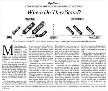
Fig. 1. The Spatial Model on the Op-Ed Page of the New York Times.

Following the mathematical exposition, we illustrate the uses of two particularly helpful NOMINATE tools: (1) DW-NOMINATE, one of the more widely used scores produced by the algorithm, and (2) Voteview, an interactive website that displays two-dimensional plots of roll calls. As with our treatment of the spatial model and the mathematics, our primary purpose is instruction—and to thereby broaden the number of participants in the NOMINATE project.

THE SPATIAL MODEL

What do we mean when we refer to a “spatial model of politics?” Consider the use of NOMINATE scores that can be found in the op-ed from the New York Times shown in Figure 1. In it, several political scientists discussed the graphic accompanying their piece that showed where major politicians could be located on a left–right continuum. As one can see, John Kerry is shown as being liberal, President George W. Bush is conservative, and John Edwards more moderate than the ideologically extreme Vice President Dick Cheney.Footnote ¹²

The basic concept that self-evidently informed the plot—namely, that politics organizes itself on a one-dimensional, left–right ideological space—is, by convention, dubbed issue space. Notice that the authors also regarded legislators as arrayed within issue space. Thus, the horizontal axis depicting issue space implicitly was broken into identical intervals correlating to degrees of conservatism or liberalism that carry actual numerical values. Finally, people in issue space evidently occupied fixed locations within it.

STARTING POINTS AND ASSUMPTIONS

The four elements of Figure 1—the assumption of left–right issue space, that the issue space has a single dimension, its underlying disaggregation into intervals, and the locational fixity of the scored politicians—underscore that there are some assumptions here about what makes individual politicians tick. Poole and Rosenthal, and those who appreciate the NOMINATE algorithm and its uses, are working with a theory of individual legislative behavior that they consider good (or at least good enough) for all legislators at all times. That theory allows for the extraction of rather precise information about ideological position from the entire, continuous record of congressional roll call votes.

At first blush, such a theory would seem not only unlikely but also wildly ahistorical. But the question is not the theory's realism so much as its capacity to order an enormous amount of information without doing undue damage to the way politicians actually behave. So let us turn to the theory.

Utility-Maximizing Legislators

One basic idea in the spatial theory of legislative behavior is that legislators, being professional politicians, know rather precisely what they want—and by the same token what they do not want out of the legislative process.Footnote ¹³ In other words, they have what is known as an ideal point when they go about their business of negotiating (or, increasingly, not negotiating.)

What do we mean by that? Consider the great function of democratic legislatures: raising and spending money. These tasks are measured and reported to everyone according to the national currency's metric, which means that democratic legislators routinely operate in easily comprehensible and metricized ways with respect to policy choices.

For instance, if a legislator prefers one level of appropriation for defense—say, a moderate hawk wishes to spend $300 billion for the current fiscal year—he or she probably would not be quite as happy with a $250 billion appropriation, and he or she would be even less happy with a $200 billion appropriation, and so forth, radiating in one direction away from the ideal point of $300 billion. Likewise, this legislator might think that a $400 billion appropriation is foolish, and that $500 billion is even more foolish than $400 billion, again radiating away (in another direction) from the ideal point.

Enter the idea of utility. A legislator gets more utility from outcomes that are closer to his or her ideal point and less utility from outcomes that are farther away from that ideal point. Additionally, this utility function is symmetric—if the legislator's ideal point is 0.5, the legislator will gain equal utility from an outcome located at 0.25 as one located at 0.75. However, the model uses squared distances to calculate utility; in other words, as the distance between the ideal point and the yea vote increases, the legislator's utility decreases exponentially.

It is not hard to see that this prosaic account is inherently spatial. A legislator derives greater utility for a legislative outcome the closer that it is to his or her most preferred outcome or ideal point. Correlatively, the greater the distance (on a dimension) of an outcome away from the ideal point, then the smaller the utility. Furthermore, it is not hard to see that for defense spending, at least, the legislator's preferences—if graphed in two-dimensional space, with “utils” (utility received) on the y-axis and spending levels on the x-axis—would execute something like a bell curve from left to right along the abscissa.

The NOMINATE algorithm uses the concept of a utility function to calculate the probability of voting yea on a bill. The idea behind the model is that if the legislator's ideal point is closer to the yea outcome than the nay outcome, then the probability of voting yea will be closer to 1. If, instead, the ideal point is closer to the nay outcome, then the probability of voting yea will be closer to 0. If the yea outcome and nay outcomes are approximately equidistant from the legislator's ideal point, then we should expect a yea vote with probability 0.5 since the legislator is indifferent between these two outcomes.

More technically (you can skip this paragraph if the words “more technically” make your eyes glaze over), the model uses the cumulative normal distribution, which is the integral of a bell curve—as the inputs increase, the probability goes toward 1, and as the inputs decrease, the probability goes toward 0, which is exactly the structure we desire. The probability of voting yea is thus expressed as $P_{ijy} = \Phi \left(\beta e^{ - 0.5\sum\limits_{k = 1}^s {w_k^2 d_{ijyk}^2}} - \beta e^{ - 0.5\sum\limits_{k = 1}^s {w_k^2 d_{ijnk}^2}}\right) $ , where s is the number of dimensions (usually 2), β and w are constants, and d is the distance between the legislator's ideal point and the yea vote or nay vote (depending on the subscript). In simpler language, the algorithm uses the difference of the square of the distance between the legislator's ideal point and location of the yea vote and the square of the distance between the legislator's ideal point and the nay vote to determine the legislator's probability of voting yea.

Now, the ideal point idea might give one the impression that legislators always get it right when they answer to a roll call. NOMINATE assumes, however, that there will be mistakes. This assumption is quite important.

Perhaps a legislator's niece—who is a dove—promised to take the legislator out to dinner at his or her favorite restaurant and then to the opera if the legislator voted for the lower appropriation, and the legislator happened to know that his or her preferred appropriation would win no matter what vote he or she cast—so the legislator voted for the lower appropriation even though that was, for him or her, ordinarily an improbable choice. Such votes do occur in a legislator's career. Additionally, at times legislators will truly make errors, perhaps due to misinformation or a simple mistake on a quick roll call they are not prepared for, which can be often enough. Legislators can answer several hundred roll calls in every congressional session, and over many sessions, the probability of some level of seemingly inexplicable voting probably grows—if only up to a certain level and no more. Every legislator has an error function, so to speak.

There is, of course, an explanation for each of the incidents of roll call behavior that seems puzzling or out of character. But a legislator's error function is not captured by the utility-maximizing spatial logic we have just laid out—hence the label error function, which refers to some residual of observations that cannot be modeled precisely. Roughly speaking, the error function allows for the possibility that a legislator will sometimes vote for an outcome that is further from his or her ideal point (ideal with respect to those issues that are included in the model) than its alternative. The spatial model is thus meant to explain only a certain amount of the variation in roll call behavior. Indeed, mathematically the spatial model needs a healthy amount of error in order to do its job of capturing variation in behavior.

Now, what comes next is a fairly challenging question. How would one know what was any legislator's ideal point in some issue space? Obviously, the legislator's roll call choices—the yeas and the nays—provide some guide to a legislator's ideal point. They communicate legislators’ revealed preferences. But here is the great difficulty: How would one take all of a legislator's yeas and nays and derive some precise measure of the ideal point? And do the same for all the other legislators? And what metric would one use?

Consider the matrix in Table 1.

Table 1. Yeas and Nays of a Three-Person Legislature

This is a very simple version of the general problem that we have just posed. This is a three-person legislature, and it has taken two roll calls, with the yea/nay outcomes noted in the column for each of the three legislators. Could one estimate one-dimensional, spatial ideal points from such a small amount of information? If so, how?

One way would be back-of-the-envelope trial and error—that is, to write down different configurations of legislator and roll call locations until one got something that made a certain amount of sense. Table 2 offers a first pass at a back-of-the-envelope trial.

Table 2. Taking the First Stab at Locating the Legislators

If you look closely at Table 2, and check what you see before you against what we have just said about ideal points and utility maximization, you will notice that A is placed rather far away spatially from A's actual votes, and C is also far away. Of the three, B is placed closest to B's actual roll calls—but not particularly close.

Is there a better configuration? Yes, one could guess the following, which involves shifting C from C's previous location on the left over toward the right and also flipping the locations of 2Y and 2N:

Notice that this arrangement, shown in Table 3, represents an improvement over Table 2: Both Legislators B and C are fairly close in space to their actual votes. But notice also that A is still pretty far away from A's second vote.

Table 3. Taking a Second Stab at Locating the Legislators

One further possibility is shown in Table 4. C is moved all the way to the right, 2Y and 2N are reflipped and moved left, B is located in the middle, and finally 1Y and 1N are put on the right. This does the most to minimize the distance between legislators and their actual roll call choices.

Table 4. Taking a Final Stab at Locating the Legislators

By this point, you get the idea. Using the information in Table 1, concerning three legislators and their roll call votes, you could map, after a certain amount of moving votes and legislators around on one line, where legislators’ ideal points probably are within this imaginary legislature. In short, one can take roll call vote information and estimate whether legislators are to the right on the whole or to the left on the whole. Thus A is to the left in issue space above, B is in the middle, and C is to the right. Or, to put it in the language of Figure 1 (recall that that is the op-ed from the New York Times) C is a conservative, B is a moderate, and A is a liberal.

Furthermore, if you wanted to develop ideological scores for these legislators, you could split the line in Table 4 into 201 intervals and come up with some sort of score for how liberal or how conservative each of the three legislators, A, B, and C, was. If the scale ran from −1 (most liberal) to +1 (most conservative), B would be about 0, A would be close to −1, and C would be close to +1.

Now we get to a harder part. If you have more than three legislators and two roll calls, then trying first this and then that obviously cannot be the way to estimate legislators’ ideal points and to generate scores. The House of Representatives has 435 members; each one runs up a large number of roll calls in a congressional session.Footnote ¹⁴ If there were two issue spaces, your head would instantly spin even thinking about the prospect of a trial-and-error effort. (Interestingly, Poole and Rosenthal actually considered making a supercomputer conduct a kind of trial-and-error iteration, but concluded that any set of instructions to the computer would cause it to produce gibberish in a short period of time, what is called “blowing up.”) In short, there has to be an efficient way to do what we did above with the actual, real-world data concerning each chamber of the U.S. Congress spanning more than 200 years.

There is such a way, and it is called maximum likelihood estimation (MLE). This is the mathematical core here. MLE obviously differs completely from the kind of trial and error that we just described—and it certainly does not involve minimizing distances per the previous exercise. So it is vital to acquire some sense of MLE in a simple version of the procedure before extrapolating to what Poole and Rosenthal did with actual roll call data in a complicated version of MLE. Our hope here—by jogging the reader's memory (or grasp) of calculus, probability, and the nature of frequency distributions—is to give an intuitive sense of what Poole and Rosenthal did to map legislators in issue space for several thousand legislators and many thousands of roll calls. Though the exposition is informal, it pays to read it slowly with stops for thinking it over.

MAXIMUM LIKELIHOOD ESTIMATION

Fitting the spatial model means choosing values for all of the parameters of the model. These consist of (1) the issue space coordinates for each legislator's ideal point and (2) the issue space coordinates for the yea and nay locations corresponding to each vote. There is also a parameter that indicates (3) the typical size of the errors. Given a complete set of these three parameter values, it is possible to compute the probability (again, based on the model) of observing any specific combination of vote outcomes.

The MLE corresponds to the set of parameters that, in turn, maximizes the probability of the observed yea and nay votes. In other words, the MLE is that estimated (i.e., the artificial or “as if”) set of legislator and vote coordinates—in the issue space—that make the real observed outcomes (i.e., the yeas and the nays that these legislators actually cast in history) as likely as possible.

To better understand the likelihood function, it is helpful to consider a problem that is much simpler than predicting the voting behavior of members of Congress. Consider a gambling device, such as a slot machine, which pays out money on any one play with some fixed probability p. To estimate p, you could play the machine 100 times and then, after each trial, record on a piece of paper whether or not money is paid out. If you assume that the probability of a success on each play equals p regardless of the outcomes of the other trials (i.e., you assume that the trials are independent of one another), then the probability of any particular combination of successes and failures is:

1. (1) Prob(observed success-failure sequence | p) = p^x (1 − p)^{100 − x} ,

where x is the number of times out of 100 that you win money (possible values of x are 0, 1, 2, …, 100). The two terms being multiplied in (1) correspond to the probability of getting x successes (each happening with probability p) and of getting 100 − x failures (each with probability 1 − p). Changing the order in which the successes and failures occur does not change the overall probability, as long as there are still x successes and 100 − x failures.

The probability statement in equation (1) treats p as a fixed number and is a function of x, the count of successes in 100 independent plays. After your experiment of playing the machine and recording your successes and failures, you will have valuable information. You will know the value of x. But you will not actually know p. To estimate it, you will need to compute a likelihood function for it.

The likelihood function L(p) is identical to equation (1), except it treats x as fixed at the observed value and as a function of the unknown parameter p. The MLE for p is the value $\hat p$ that maximizes L(p). In other words, $\hat p$ is the value of p that makes what happened (observing exactly x successes) as probable as possible. This does not mean that it is the correct value of p; other values close to it are nearly as plausible, and there is no ruling out the possibility that something incredibly improbable (e.g., a run of good or bad luck) happened on your sequence of trials. However, MLEs are optimal estimators in many ways, and much is known about their behavior, particularly when the number of trials is large.

For example, suppose you win 10 times out of 100 plays. The probability of any particular sequence that includes 10 successes and 90 failures is L(p; x = 10) = p ¹⁰ (1 − p)⁹⁰, which is plotted in the top half of Figure 2. This likelihood function is maximized for p = 0.1, with the result that $\hat p = 0.1$ is the MLE. The maximization can be seen visually in the simple example plotted in the top half of Figure 2 for 100 trials. In the second graph, at the bottom of Figure 2, the MLE is also $\hat p = {\rm } 0.1$ , but the number of trials depicted is 1,000, 10 times the number for the graph in the top half. In this scenario, with x successes in n independent trials, the MLE is x/n, the observed proportion of successes. But with the larger number of trials, the range of plausible values that might be the true probability is narrower. (The differences between the rectangles underneath the curves emphasize that.) The relative accuracy of the estimates thus increases as the number of trials increases. The analogue for NOMINATE would be to have the results of a larger number of votes.

In other words, with more information we narrow the range of plausible estimates—which is what we want. The rectangles in Figure 2 show 90 percent confidence intervals for p corresponding to n = 100 and to n = 1,000 with $\hat p = {\rm } 0.1$ in each case. The first interval is larger by a factor of roughly $\sqrt {1000/100} $ , or about 3, meaning that around three times as many values of p must be considered plausible when using 100 trials compared to 1,000 trials. But using a larger sample size will reduce the number of values of p that can be considered plausible—which means, in turn, greater accuracy and precision.

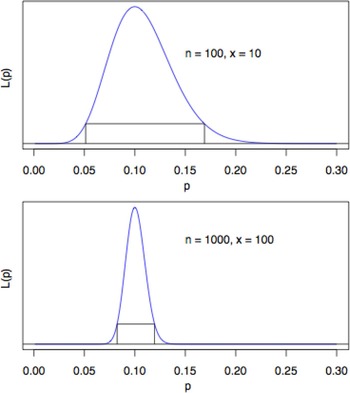
Fig. 2. Visualizing MLE.

All of this brings us to a strength of NOMINATE. The above examples have only one parameter and 100 or 1,000 outcomes. But NOMINATE routinely fits models with many thousands of parameters and outcomes.

Each person who has voted in a Congress has one or several associated parameter values (coordinates in issue space), as does each question that was voted on. How might we analogize these legislative facts? Imagine that there are 600 different gambling machines (our analogue for an arbitrary number of roll calls, i.e., 600) and, further, imagine that the machines may have different characteristics (e.g., different p values). Now suppose there are 435 different people playing each machine, and that the players differ from each other at the business of winning money. In other words, the probability of a player winning on a particular play depends on both the player and the machine being played.

The different players in this example obviously represent different members of the U.S. House, and the different machines would—pursuing the analogy—represent different questions being voted on in a Congress. Voting yea on a question, in turn, would correspond to winning money on a play, and its opposite, voting nay, would correspond to losses.

Given values for all of the voter and question parameters, Poole and Rosenthal devised a function for the probability of votes being cast in a particular way. This function defines the likelihood L for the set of parameters, and the MLE is the combination of voter and question coordinates that result in the largest possible value of L.

Now, there are important complications that require notice. Complications arise due to the large number of parameters involved in the Poole-Rosenthal likelihood function (i.e., recall that the T and E in NOMINATE stand for three-step estimation). To estimate the parameters, Poole and Rosenthal separated the parameters into three groups: the estimates of the roll call parameters, or the spatial locations of the yea and nay outcomes of each vote; the estimates of ideal points of each legislator; and the scaling parameters that determine the shape of the legislators’ utility functions. The NOMINATE algorithm holds the estimates of the ideal points and scaling parameters constant while estimating the roll call parameters, then holds constant these new estimates of the roll call parameters and the scaling parameters to estimate the ideal points, and then holds constant the estimate of the roll call parameters and the new estimates of the ideal points to estimate the scaling parameters, and so on. The algorithm cycles through estimating one group while holding the other two groups constant until it converges upon estimates for the three groups of parameters. Even then, each of these groups of parameters is very large, and estimating them is not simple. While there is an explicit formula for the MLE in the simple example with the slot machine, Poole and Rosenthal used much more computationally intensive methods. How exactly did they do this?

They used a computer algorithm (for those who are interested, it is the BHHH gradient algorithm) to handle the massive amount of information with which they worked. What did that involve? Here is another analogy: Think of a very, very large and bumpy field with lots of little hillocks of varying height. There are, very roughly, three dimensions in this large terrain: length, width, and height. Your job is to find the highest location in this hilly field. This is like finding the MLE for a two-parameter model. The third dimension, height, represents the value of the likelihood function for any particular two-dimensional location in the field.

Now, for the one-dimensional NOMINATE model, the highest hill would be located over a space of dimension equal to the number of legislators plus two times the number of votes—which is the total number of parameters in the model. A two-dimensional NOMINATE model would, of course, have twice as many parameters as the one-dimensional model.

To find the highest point in the field, you could check the height of every possible location with an altimeter and identify the maximum. However, this procedure could take a very long time if the field were large—which, given the number of Congresses and roll calls, it obviously is. A faster method would be to start in some location, and then take a step in the direction that increased your height the most. From this new position, you could take another step in the direction that again gave you the largest increase. After many steps, you would eventually arrive at a location from which you could not go any higher. You would then conclude you were at local maximum. Repeating this gradient method from various starting locations, you could be reasonably confident of identifying the overall highest point in the field. This would, in fact, be a very tiny bit like the trial-and-error example above—although in fact you would be using a form of mathematics called hilltopping in higher dimensions.

To use this procedure with the NOMINATE model, you first choose a starting set of parameter values, θ (the coordinates in issue space for the legislator ideal points and all of the yea and nay locations), and calculate the likelihood function, L(θ). Then you move to a slightly different set of values, and evaluate L(). If L() > L(θ), you accept it as the new θ. In this way, you keep moving in the direction of the gradient vector. Repeating this procedure many times allows you to climb the hill until you arrive at the value that maximizes the function L, at least locally.

It might be helpful here to summarize by reconsidering the simple case in Table 1, repeated below.

Recall that we tried fiddling around with getting the appropriate relative distances between possible ideal points and the yea and nay points, even with only three legislators. We thus did very roughly (and without the mathematics of probability) what NOMINATE does systematically with much, much more information—and, quite crucially, using probability (not distance minimization).

But we can actually use MLE on this simple three-legislator example—and that would help us to close out our mathematical overview. Suppose we knew two groups of the parameters in our example—the scaling parameters and the roll call locations. Then we could easily use the likelihood function to estimate the ideal points of the three legislators. We will let (what are known as) the scaling parameters β = 5 and w ₁ and w ₂ = 1,Footnote ¹⁵ as these are reasonably close to the estimates that Poole and Rosenthal usually estimate. We will estimate the roll call locations to be similar to those in Table 4; that is, we will let 1Y = 0.3, 1N = 0.7, 2Y = −0.3, and 2N = −0.1. The likelihood functions of the ideal points for Legislators A, B, and C given these parameters are shown in Figures 3, 4, and 5.

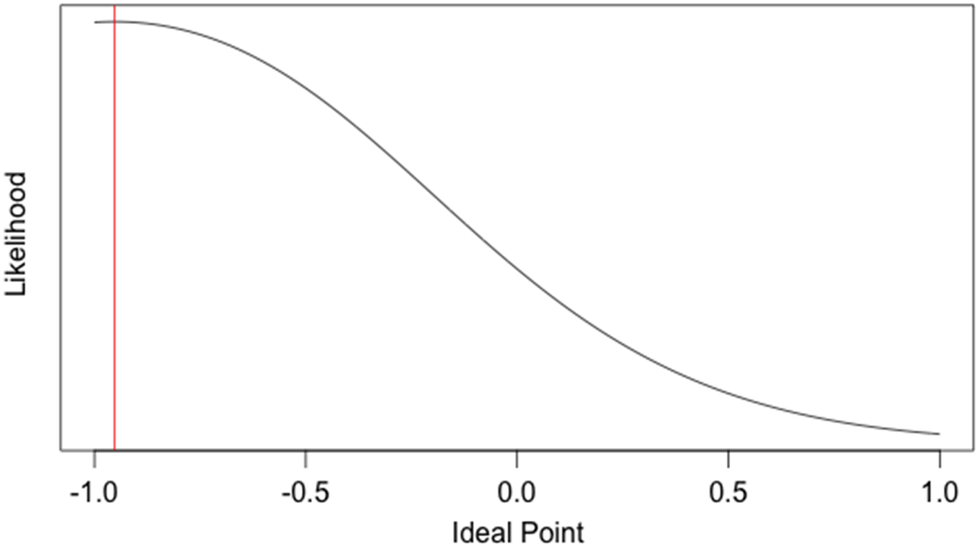
Fig. 3. Maximum Likelihood Plot of Ideal Point for Legislator A (YY).

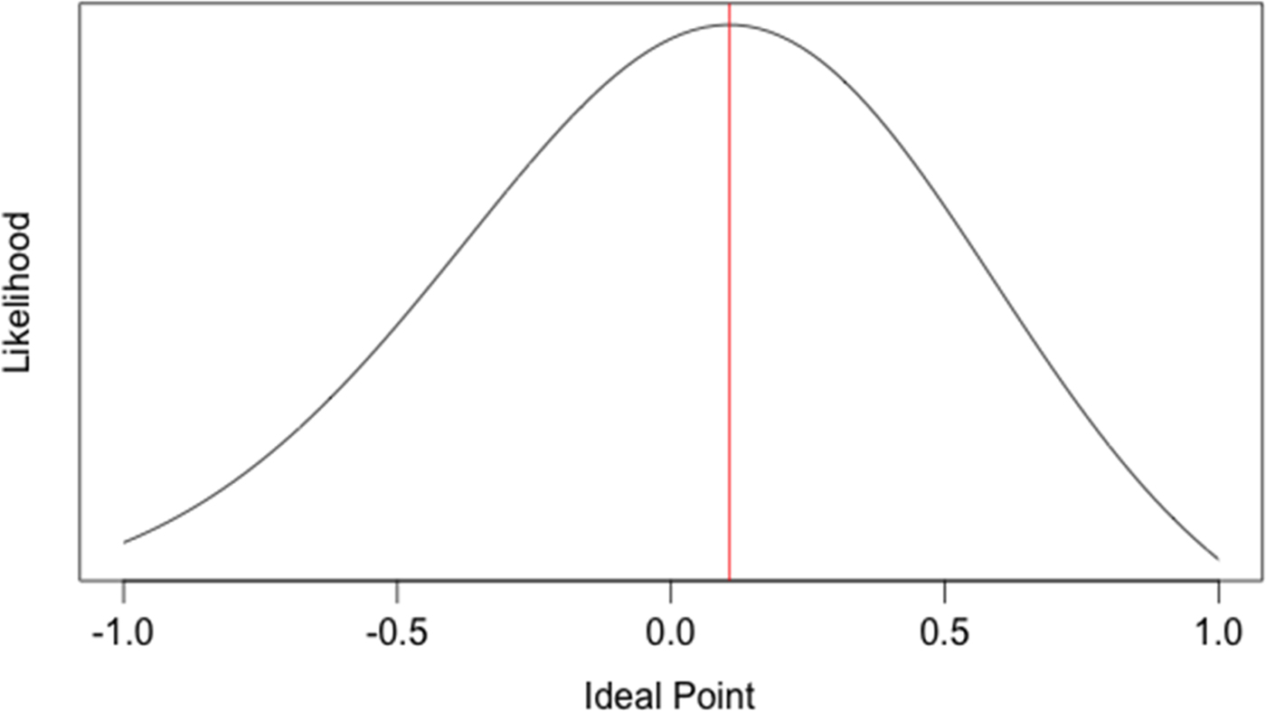
Fig. 4. Maximum Likelihood Plot of Ideal Point for Legislator B (YN).

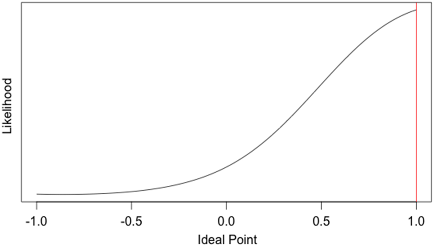
Fig. 5. Maximum Likelihood Plot of Ideal Point for Legislator C (NN).

The red vertical lines on each plot represent the ideal point at which the likelihood function is maximized; in other words, this is our best estimate of each legislator's ideal point. A plot of these estimates along with the roll call locations together on a single dimension is shown in Figure 6.

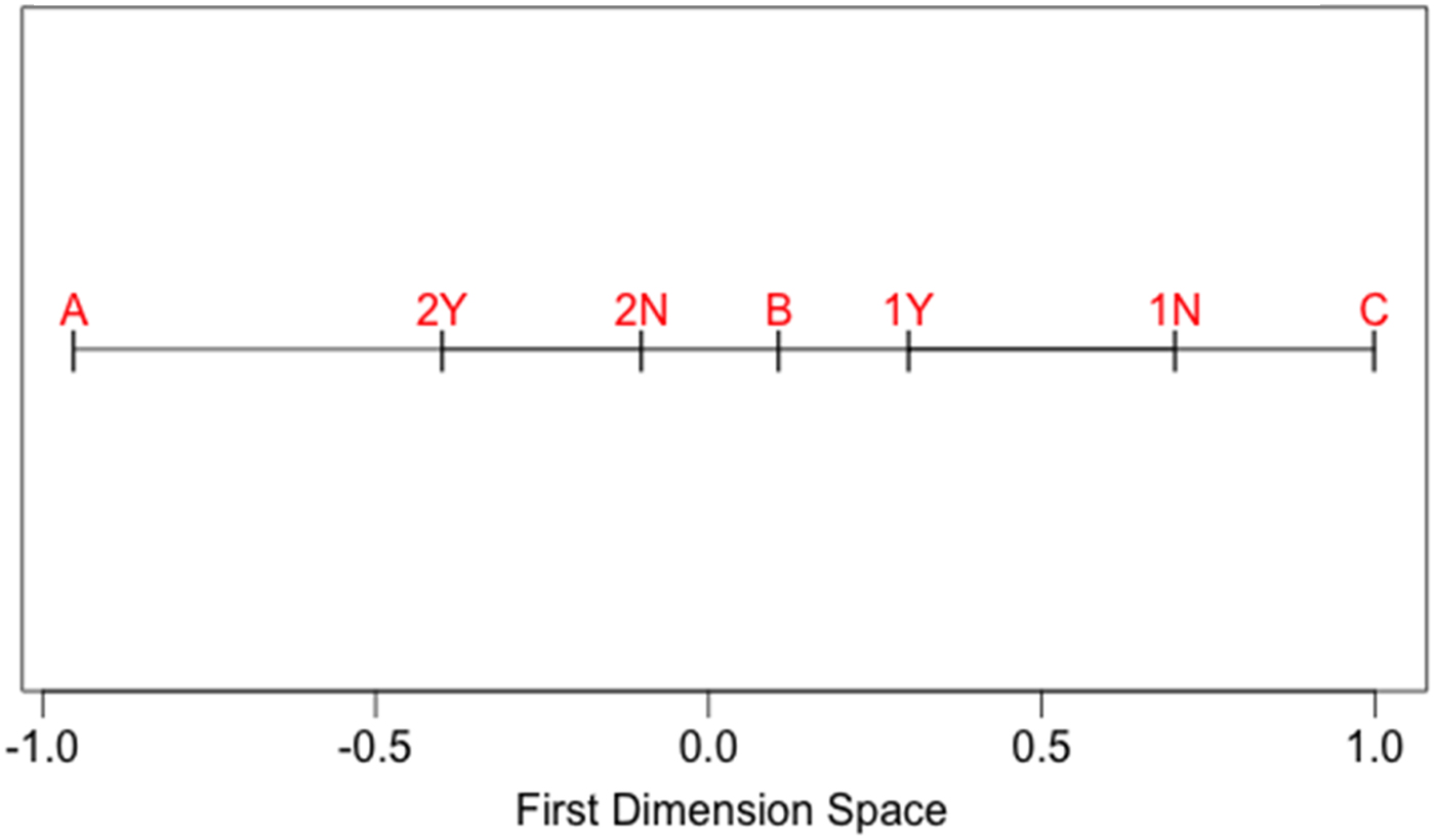
Fig. 6. Roll Call Positions and Legislator Estimates.

The MLE estimate of the locations of Legislators A, B, and C are very similar to those in Table 4 using trial and error. One notable difference is that the MLE estimate for Legislators A and C are more extreme than the trial-and-error estimates—in fact, they are very close to −1 and 1, respectively. This is because of the nature of the quadratic penalty in the normal utility function—if a legislator votes almost perfectly in a conservative or liberal way, the legislator's score can blow up (which is why the DW-NOMINATE algorithm, a version of NOMINATE, constrains scores to be between −1 and 1 on all dimensions).

To recapitulate, in NOMINATE any given set of estimated coordinates for legislators in one or two issue spaces yields a certain probability of the observed votes. The MLE is the set of coordinates for all legislators in a Congress or in an historical period that makes this probability the largest. We tried to get the likely issue space locations of three legislators by fiddling with their observed yea and nay votes by trial and error, but NOMINATE does this for thousands and thousands of legislators and their roll call votes through hill climbing. Once a solution is obtained, that is, once NOMINATE thinks it has found the highest point in the hilly field, the legislator and roll call parameters that are associated with that decision—which are the estimated coordinates—are dropped into a metric of some sort that can be easily interpreted (e.g., a scale between −100 and 100). The resulting scores are the NOMINATE scores available on the voteview.com website for each member of Congress since the First Congress.

It was a slight variation on these scores that the authors of the 2004 op-ed (see Figure 1) were using in order to make the claim that together Kerry and Edwards were less extreme than Bush and Cheney.Footnote ¹⁶ They got Bush's NOMINATE score by treating his legislative messages—up or down on policy questions—as one more set of yeas and nays in the legislative process. These were simply added into the database on which the algorithm worked. Cheney's scores did not equate with Bush's, but instead the authors probably used his roll call votes from his time as a member of the House.

THE DEBATE ABOUT WHAT THE SCORES ACTUALLY MEASURE

It cannot be stressed enough that all of the very closely correlated versions of NOMINATE scores are not true values of anything real. They are merely estimates of (legislators’) parameter values that govern a probability model used to approximate nonrandom, real-life outcomes. Legislators and roll calls have specified locations in a postulated issue space, and they—and the postulated issue space—can be mathematically recovered given roll call votes for each legislators and through a data-reduction algorithm. The fitted parameters of the model form the basis of the scores.

But as Figure 1 suggested, these scores clearly seem to tell us something important about real people. In that case, they seemed to show how far apart politicians were ideologically and the extent to which they were conservative or liberal. This view of the NOMINATE scores holds that, at bottom, congressional politicians are engaged in programmatic struggles. Polarization indicates philosophical disagreement about what government is for. Politicians fight each other because they care about their very different ideas about what the big social, political, and economic problems are—and about what facts concerning these problems matter and do not matter. Politicians’ battles receive a great deal of assistance, in fact, from pundits and public intellectuals. Such “idea brokers” help to construct what the terms “conservative” or “liberal” stand for at any particular moment in American political history.Footnote ¹⁷

Another view of the scores holds, however, that we need to weigh carefully just how much the scores really reflect ideological disagreement or overlap. On this view there are periods in American political history in which partisan contestation—qua organizational combat in order to gain and hold office—can be fiercer than at other times. We are in one of those times. Changes in the scores since the late 1970s reflect that growing ferocity—and politicians’ creative proliferation of hardball tactics. Partisan majorities and minorities might be using the legislative agenda mainly to sharpen their partisan (not ideological) differences. The war of ideas, while clearly salient, is not the sole or primary determinant of combat.Footnote ¹⁸

We can hardly resolve this debate—but the larger points are, first, that there is a debate and, second, that users of NOMINATE scores should be cautious in using and interpreting the scores. Delving into historical context and careful qualitative (or even text-as-data) investigation of rhetoric and motivations clearly matter—which means that APD scholarship is essential for the proper use of NOMINATE scores.Footnote ¹⁹

DIMENSIONS AND SCORES—AND THEN A VOTEVIEW LOOK AT THE NEW DEAL

NOMINATE and APD can, in fact, form many kinds of partnerships. To illustrate that point, let us consider the scholarship that treats whether and how Southern Democrats strongly shaped the New Deal's social policies. Since the late 1970s and early 1980s, many scholars have explored how the division in Congress between Northern and Southern Democrats affected New Deal policy design in ways that hurt the interests of African American citizens.Footnote ²⁰ They have asked: Was New Deal social policy designed to block out or exclude African Americans from the benefits of the emerging welfare state? Was New Deal social policy meant for whites first and for blacks only second?

How might one dig into these questions using NOMINATE? The first step is recognition that politics during the New Deal (and indeed for all of American political history) has been not one dimensional but two dimensional. You will have noticed that most of our discussion has assumed that politics is one dimensional and that we have referred only here and there to the obvious possibility that there may be more dimensions to politics, including a second dimension. We now posit that there are in fact two dimensions. It turns out that this was a discovery of the NOMINATE algorithm; that is, NOMINATE revealed that besides a first dimension, there is a second dimension in roll call behavior. In fact, the most basic finding of Poole and Rosenthal is that American politics has almost always exhibited low dimensionality—by which they mean no more than two mathematically recoverable issue dimensions.

To recall, these dimensions are purely formal. This is exceptionally important because it means that every significant substantive issue “loads” (in the language of factor analysis) onto one or the other of the two dimensions. But that is of course very odd! There is a very wide range of seemingly disparate issues in contemporary American politics—from gay marriage to environmentalism to “intelligent design” in secondary science education to land use to gasoline prices to foreign policy to immigration, and so on. Undoubtedly, the same was true in the past. Furthermore, such results as the Condorcet paradox and the McKelvey chaos theorem dramatize both agenda instability and the potentially very large dimensionality of majority rule.

How can it be, then, that there are only two, truly basic issue dimensions in U.S. politics? The Poole and Rosenthal answer is, in effect, surprising, but altogether true. They fit a model with one dimension, to see how successfully that captured legislative behavior. Then they fit two dimensions, to see how much that improved the model's performance, then three dimensions, and so on.Footnote ²¹

They found that the one-dimensional model was about 83 percent accurate overall, meaning that in 83 percent of all the individual votes, the legislator voted for the outcome whose position in issue space (as estimated by NOMINATE) was closer to the legislator's ideal point (again as estimated by NOMINATE), while the two-dimensional model was about 85 percent accurate. Three or more dimensions offered virtually no improvement over two, which implied that Congress's issue space has nearly always been no more than two dimensional, at least to the extent that a spatial model can approximate ideal points in congressional roll call voting over time. As for the other 15 percent, it is nondimensional voting lacking any underlying structure—pork-barrel voting and error (as in the discussion early in this article).

Poole and Rosenthal did not, it should be noted, directly estimate the number of dimensions. Instead, what they did was assume that the issue space had been one dimensional and then fit the model to the data. Then they assumed a second dimension. Ex ante, the improvement in fit (called average proportional reduction of error) had to grow. What they did was a bit like throwing another independent variable into an ordinary least squares regression—R-squared will always go up, even if only a bit, no matter what plausible variable you add. Assuming a second dimension doubles the amount of information you are working with. Rather than running a climb-the-hill algorithm in an east–west space, or north–south space, one runs it in a space that has both an east–west plane and a north–south plane, so there are now twice as many local maxima to climb, which, in turn, can do only one thing to your estimated parameter values for your legislators—because you now have two more coordinates for each—namely, kick these estimated values closer to the real values.

Their cleverness, though, lay in trying to gauge how much change one got from this trick. That it was only 2 percent was remarkable. Then they did the trick again and nothing changed, really.Footnote ²²

This idea of just two dimensions also makes substantive sense out of long stretches of American political history. We can see this point clearly if we think of the Southern New Deal Democrat, a legislator who voted for liberal economic positions but voted against anti-lynching legislation. This was a legislator who operated on two dimensions regularly. On one dimension, he was a liberal; on the other, he was the opposite of a liberal: he was a conservative.

What this further means is that every legislator during this period (indeed in all periods) has two scores: first dimension and second dimension. To illustrate how legislators within the same party might differ from each other on the second dimension, we have listed what are known as the DW-NOMINATEFootnote ²³ scores for Massachusetts and Mississippi Democrats for the 74th Congress.

Figure 7 displays the relevant DW-NOMINATE scores for the Massachusetts and the Mississippi delegations in the U.S. House for the 74th Congress. Looking at Congressman McCormack from the 12th Massachusetts district (later Speaker of the House), one sees that he locates somewhat toward −1 on a scale of economic liberalism and conservatism running from −1 to +1. His Republican colleague from the 4th District is far more conservative than he is, as indicated by his score of 0.352.

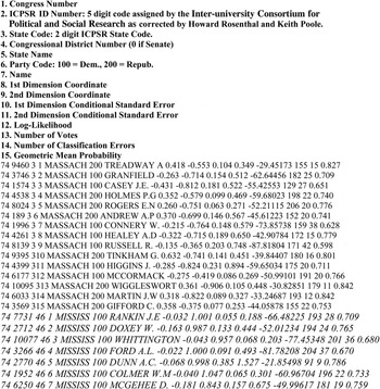
Fig. 7. DW-NOMINATE scores for the Massachusetts and the Mississippi Delegations, 74th Congress.

Looking at the Mississippi Democrats, one sees that they are less economically liberal than their Massachusetts counterparts. Also, they are more conservative on the second dimension. Indeed, Congressman Rankin is maximally conservative on the second dimension, that is, with regard to policies that would change race relations in Mississippi, placing him at +1.Footnote ²⁴ McCormack, for his part, is relatively liberal on the second dimension.

By now we are very close to the lively debate about whether the New Deal further entrenched black disadvantage through its broad social programs. Consider the design of the 1935 Social Security Act: Were agricultural workers deliberately left out of the original coverage of the act in order to accommodate the preference of Southern Democrats that black landless workers not receive federal protection in the form of old age income security? At the time of the bill's passage, the NAACP pointed out the gap in coverage. On the other hand, no Southern Democrat clearly and unmistakably voiced a desire that the act's coverage features not disturb Jim Crow. Also, the Secretary of the Treasury, Henry Morgenthau, underscored the enormous administrative difficulty of implementing the act if it were written to cover agricultural and domestic workers—and tightly focused revisionist research has shown that this argument was not pretextual.Footnote ²⁵

NOMINATE has a spin-off that throws interesting light on the issue—Voteview. It is a very powerful tool. For a long time it was available as software for download from the Voteview website to a PC (but not to a Mac). Many scholars still have this “legacy software” on their PCs. But thanks to the ingenuity of Jeffrey Lewis and a team of collaborators, it has again become available to everyone, this time as an interactive web tool that works with both PCs and Macs (http://voteview.polisci.ucla.edu/).

Voteview displays (among the dozens of features that it has) spatial plots of roll call votes. The plots that are shown in the next few figures are from the legacy software—so they do not look quite like the ones that you will be able to get on your own by searching the site.Footnote ²⁶ But they are close enough to what you will be able to find on your own for us to discuss.

Back to the question at hand! Visual inspection of the legacy Voteview plots that we generated in 2004 yields useful information on whether Social Security was covertly exclusionary. Why? Because NOMINATE is expressly set up to detect not one but two dimensions—and the second dimension in this period is, plausibly enough, racial. In other words, one would expect a vote on Social Security to display the patterning that one would see in a vote that taps the second dimension. But it does not—and that reframes the discussion about Social Security. First, though, a quick Voteview tutorial.

A Brief Tutorial on Voteview

Each spatial display provided by the older Voteview software had several useful features. It showed clouds of tokens, each of which represented a particular legislator. That is also the case with the new interactive software. In the older version the tokens were labeled either R, D, or S for Southern Democrat, and they were color coded. (As of this writing, the interactive site just shows colored dots in clouds.) For both versions, the clouds are bunched or dispersed in a wide variety of ways. Such bunching or dispersion roughly indicates partisan or factional cohesion along one of the two NOMINATE dimensions—and the patterns of bunching or dispersion also reveal how dominant the first dimension is in any particular vote.

In this connection, consider Figure 8, which displays a House roll call on April 15, 1937, to amend a bill criminalizing lynching. Rep. Howard Smith of Virginia proposed an amendment to this bill: It proposed striking out the sections of the bill that imposed fines on counties in which lynchings occurred. As one can see in Figure 8, almost all of the S tokens (for Southern Democrats) are above the line (we say more about “the cutline” shortly), and many of the other party-label tokens (R, D, and F) lie underneath the line in two clouds.

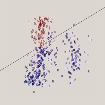
Fig. 8. Anti-Lynching Bill Roll Call Vote, April 15, 1937.

The cutline thus shows that the vote on Smith's amendment was a second-dimension vote—but the small cloud to the right, underneath the cutline, also indicates that the Republican and Democratic parties had a polarized relationship to each other on the ordinarily dominant first dimension. (Note that you will not see a cutline in the new software; instead, the angle of the cutline is available for download, and you can also visually estimate it by looking at the space—or channel—between clouds of dots.)

Now to the cutline. NOMINATE assumes that the question voted upon has yea and nay positions in two-dimensional issue space. The yea and nay locations of the question are unknown parameters. The yea and nay coordinates of the legislators are also unknown parameters. All of the locations are found by maximizing the overall likelihood function for all of the unknown coordinates. The cutline is a line perpendicular to the line joining the NOMINATE-estimated yea and nay points of the question voted on. This (perpendicular) cutline furthermore bisects the other (joining) line at its halfway point. There are misclassifications—NOMINATE is, after all, likelihood estimation. But those legislators whose issue space positions make them likely to vote yea are typically on the yea side of the cutline, and vice versa. Here the yeas are blue, the nays are red, and the misclassifications are either blue or red tokens that will stand out visually.

As an aside, when a legislator is misclassified by NOMINATE (and thus by its visual front-end, Voteview) the initial hypothesis is always that the legislator's relative indifference to the outcome of the vote was higher than it was for his copartisans or factional colleagues. But Voteview will allow you to inquire about a misclassified legislator—and the result may prompt further useful speculation beyond the standard initial hypothesis.

There is even more information to be had from the cutline or the visual channel that you will notice. Looking at it in Figure 7, the anti-lynching roll call, one notices that it tends toward the horizontal. This particular angularity is in fact quite significant. The flatter a cutline is, the more likely the vote is a second-dimension (north–south)Footnote ²⁷ vote. By the same logic, the more vertical the cutline is (as we will shortly see in considering the display of a vote on Social Security), the more likely the vote is a first-dimension (east–west) vote—that is, much like the one-dimensional plot of the very first figure we presented (i.e., Figure 1). A perfectly horizontal cutline would indicate that variation in the second dimension completely drove variation in voting behavior while one's first-dimension location would be irrelevant, and a perfectly vertical cutline would indicate that variation in the first dimension completely drove variation in voting behavior while one's second-dimension location would be irrelevant.Footnote ²⁸

Was Social Security Covertly Racialized?

Let's turn now to Social Security in particular. Recall that the NAACP criticized the proposed design of the Social Security Act of 1935 for its initial lack of coverage for farmers, farm laborers, and household workers and servants, on the ground that this feature of the act's design would leave about half of all African American wage earners unenrolled in the program. Several policy scholars have taken this criticism seriously enough to infer racial intent in the act's design.

Sean Farhang and Ira Katznelson, for example, point out that the number of cases of clear Southern Democratic racial animus in designing policy that would affect the income, education, and work conditions of black Southerners is large. Given the regularity of the pattern, they suggest that it makes sense to also code Social Security as belonging to this larger set of covertly exclusionary policies.Footnote ²⁹

But there is no strong direct evidence—actual smoking-gun statements—of racial animus on the part of Southern Democrats—whereas with the other policies there is. Social Security could be sui generis—in a set of 1, all by itself. Indeed, Larry DeWitt, Gareth Davies, and Martha Derthick have strongly argued that administrative necessity better explains the initial restriction of the act's coverage formula to urban and industrial wage earners.Footnote ³⁰ This point reminds us that in 1935 the United States was a much more agrarian nation than it is now. Huge regions of rural America were quite remote. Furthermore, these areas were mired in a deep economic crisis with no certain outcome. To ask effectively bankrupt farmers to administer the Social Security system of contributory finance on behalf of their tenants—an organizational matter that today we rarely notice as we clock in at highly bureaucratized, modern workplaces—would have been, once one reflects on the matter, very hard and certainly politically costly for the Roosevelt administration.

Can Voteview adjudicate the difference between these rival scholarly views of Social Security? Considerations of space preclude a full application of Voteview to all of the relevant roll calls and to inspecting the angles of the cutlines and displaying information about them in, for instance, a plot or in histograms. But two more applications of Voteview do suggest that such a fuller exploration might well be informative.

Figure 9 displays a House vote from April 11, 1935, on an open rule to permit 20 hours of debate on H.R. 7260, “a bill establishing a system of social security benefits.” The verticality of the cutline suggests an almost perfect first-dimension roll call with little evidence of the hidden racial dimension criticized then by the NAACP and since then by many policy scholars.

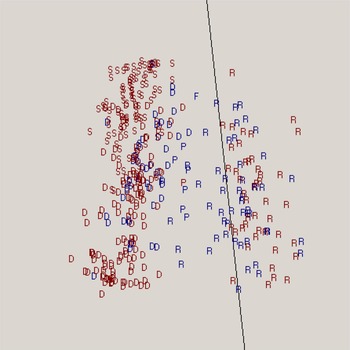
Fig. 9. Roll Call Vote on an Open Rule to Permit 20 Hours of Debate on H.R. 7260, April 11, 1935.

Also consider Figure 10, which displays the structure of a December 17, 1937, House vote on a motion by a conservative Republican, Fred Hartley of New Jersey, to “recommit S. 2475, an act providing for the establishment of fair labor standards in employments connected with interstate commerce.” The Fair Labor Standards Act was generally understood to exempt agricultural labor, an exemption that Northern and Southern Democrats in both chambers collaborated on. Several Southern Democrats openly expressed concern about the impact on race relations in the South if Congress followed FDR's original proposal to have the Fair Labor Standards Act (FLSA) cover both agricultural and industrial labor. Nonetheless, the Senate failed to specifically expand the agricultural exemption for tobacco, cotton, and seasonal activity, though it did so for dairy and the packing of perishable goods, and for packing and preparation in the area of production. It is interesting (see Figure 10) that the vote on Hartley's successful motion to recommit has a noticeable second-dimension/north–south structure to it of the kind that one sees in Figure 8. (That the cutline tips to the left, rather than to the right, is irrelevant, incidentally.)

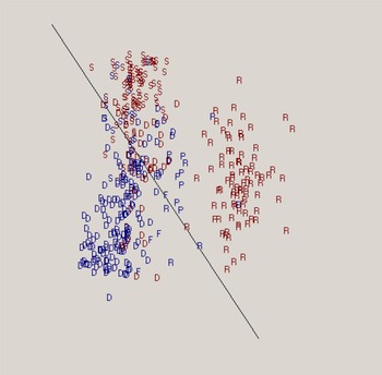
Fig. 10. Roll Call Vote on a Motion Regarding Fair Labor Standards, December 17, 1937.

The upshot here is this: Using one of NOMINATE's tools—Voteview—raises the intriguing possibility that Davies, Derthick, and DeWitt are right: Social Security, unlike the FLSA, was not covertly exclusionary. Why? We cannot say for sure—but here is a sketch of what might be the right answer. Social Security may never have threatened the Southern political economy in the same way that the FLSA did. Social Security would take many years in the future to pay out—or so it was widely thought at the time. Only later was the payout schedule accelerated. Second, everyone in the debate may have assumed that the program was geared for the industrial economy of the 1930s, not the entire American economy.

It is only today, after decades of experience with non-means-tested, contributory finance programs, which have a universal application, that as a country we are much more likely to aspire to start programs as close to their universal level as possible (i.e., 100 percent of the population). Indeed, that assumption was a major sticking point in the 1993–94 debate over health insurance, and it was interestingly never open to serious debate. The Patient Protection and Affordable Care Act (“Obamacare”), similarly, is about expansion of health care coverage—it aims for universality.

But Social Security was not initially a universal program. It has become effectively universal only over the long run. The program was instead designed to be a targeted program at its inception, and the target population was the adult male wage earner in a corporate setting who was likely to have a stable, lifetime job with a career ladder. Very few Southern workforce participants, white or black, were in that initial conceptualization of the target population precisely because the South was rural. On this view, Social Security was, as Davies and Derthick suggest, never meant to apply to rural America—and the verticality of the cutline is consistent with that conceptualization of the program.

To be clear, we do not claim to have settled the debate about whether Social Security was covertly racialized legislation—as the NAACP charged at the time. We have really only weighed in on one side (and not, we might add, entirely happily given that we hardly like to dispute the NAACP's contemporary judgment—we only went where the evidence took us!). Settling the debate about Social Security will probably require yet more archival research. But this is the point: Voteview and NOMINATE open up new vistas for APD scholarship on social policy.

POLARIZATION IS DEVELOPMENT

As we suggested earlier, there are many possible points of contact between APD and the NOMINATE project. Perhaps the most pressing and relevant to public affairs is making sense out of our contemporary polarization. Consider Figures 11 and 12 (which were drawn from the Voteview website). They visually offer one way to define polarization, namely, change in the percentages of noncentrists in either chamber of Congress over time. These have sharply increased.

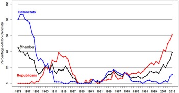
Fig. 11. Senate 1879–2015: Position of Noncentrists (less than −0.5 or greater than 0.5) in the Parties on Liberal–Conservative Dimension.

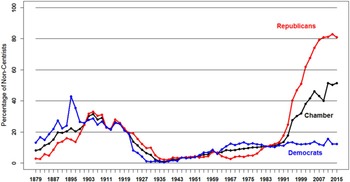
Fig. 12. House 1879–2015: Position of Noncentrists (less than −0.5 or greater than 0.5) in the Parties on Liberal–Conservative Dimension.

The emergence of such division at the top of the political system is having a wide range of collateral effects beyond Congress.Footnote ³¹ First, the change seems to be partly sorting some citizens into different ideological camps—and that may be part of why politicians appear to pay less of a penalty than they should for outrageous assertions or stating falsehoods. There is a sharp debate about this to be sure. Some argue that the public is not particularly polarized—and that it is best called a “purple America.”Footnote ³² If so, there is a very serious disconnect between the ideological intensity in Washington and the rest of the country. Either way, the interaction and contrasts between professional politicians’ signaling and position taking and ordinary citizens’ attitudes and views are increasingly disturbing.Footnote ³³

Second, hyperpartisanship has affected the staffing of the federal judiciary—and the Supreme Court itself. In a less polarized time there would be nothing like the remarkable election-year stand-off of 2016 over President Obama's nomination of Judge Merrick Garland to the seat on the Court vacated by the death of Associate Justice Antonin Scalia. The effectiveness of the administrative state also seems to be at greater risk—as Sarah Binder and Mark Spindel have argued in their study of congressional attacks on the Federal Reserve.Footnote ³⁴

Third, divisions at the top mean that some pressing policy problems are piling up without political resolution. As polarization has increased, so has income inequality—yet policies that might lower income inequality are taken off the table by the impossibility of bipartisan agreement on, for example, increases in the minimum wage and the enhancement of the administrative and enforcement capacity of the Wage and Hour Division of the Department of Labor, which polices wage theft.Footnote ³⁵ Some argue that, perversely, polarization favors policies that significantly increase income inequality.Footnote ³⁶

Also, major policy reforms (such as Obamacare and the Dodd-Frank Act) face much sharper attack and backlash than they otherwise might. An ever-growing community of journalists, legal academics, economists, and political scientists are concerned by polarization's effects on fiscal policy, as well. Fiscal disorder may have an independent effect on macroeconomic performance.Footnote ³⁷

For all of these reasons (and others) our contemporary polarization is widely (though not universally) regarded as a serious pathology.Footnote ³⁸ Yet, oddly enough, as Nolan McCarty and Michael Barber have pointed out, we do not fully understand why polarization emerged when it did, why it did not slow down and instead grew steadily, and why depolarization today seems so unlikely. So far, widely held assumptions—gerrymandering caused it, the transformation of Southern politics caused it—have been falsified. Also, exacerbating factors have been identified. One of these is the relationship between campaign finance and weak party control of candidacies.Footnote ³⁹ Another is the asymmetry in polarization: Republicans have marched rightward since the 1970s, but Democrats have not moved left since that time to the same degree (as Figures 11 and 12 show).Footnote ⁴⁰ The obvious liberalism of the Democratic party today is an artifact of the disappearance of conservative Southern Democrats, not of Democrats polarizing (except very recently and only slightly in the Senate) along with Republicans. But despite these analytic gains, the basic puzzles of timing, relentless growth, and the improbability of depolarization remain.

One strategy for addressing these puzzles involves bringing in the states and looking for variation among the states in timing of polarization in state legislatures, pace of polarization, and degree of polarization.Footnote ⁴¹ Another strategy, however, for cutting into these basic puzzles is closer to APD's core strengths: comparison of the present to previous national periods of polarization and depolarization.Footnote ⁴² To do this, APD scholars could construct a full series. The plots in Figures 11 and 12 begin in 1879. We need a series from the early Republic to the present—not an easy matter, given that NOMINATE distinguishes between pre–Civil War and post–Civil War Congresses. But if the problems in comparability could be addressed then such a series would enlarge N beyond the current option of comparing two polarizations and observing one depolarization. Once we have identified the universe of cases, historically oriented scholars would be well positioned to contribute to the polarization discussion. For example, they could investigate the ideational and institutional forces associated with the full oscillation of polarization and depolarization over American history—and how much the national series reflects three possibilities or some combination of them: sheer partisan combat, how parties structure the roll call agenda, and ideological warfare.Footnote ⁴³

APD scholars could also address whether depolarization involves trade-offs. The obvious trade-off that Figures 11 and 12 suggest is that depolarization for much of the twentieth century depended on taking racial hierarchy and discrimination and even white-on-black extra-legal violence off the congressional agenda. Were there similar trade-offs earlier in APD? What do they suggest about prospects for depolarization today? There seems to be a strong case for the formation of a multiyear, well-funded working group oriented toward producing an edited volume about how APD specifically can contribute to the current polarization discussion.