


1. Introduction
Flow separation is the detachment of a viscous fluid layer from a body surface. It results in flow reversing its direction and is effectively driven by an adverse pressure gradient, which may arise due to significant regions of surface curvature such as corners on a body's surface (in the case of external flows) or geometry constrictions (in the case of internal flows); an excellent description of flow separation can be found in Sychev et al. (Reference Sychev, Ruban, Sychev and Korolev1998). Amongst other potential negative impacts, flow separation can directly lead the flow to transition from a laminar to a turbulent state, which in most cases is considered detrimental (Hanks Reference Hanks1963). In aerodynamics, flow separation significantly impacts lift, and laminar–turbulent transition contributes to an increase in the friction component of drag. In particular, skin-friction drag is one of the largest contributors to aerodynamic drag in commercial aircraft. The implications of such increases thus impact globally on both an economical and environmental level. Although fuel efficiency is one of the main concerns in the aircraft industry, requirements on environmentally friendly transports are providing an added impetus for more fuel-efficient aircraft.
Studies of laminar–turbulent transition, with the aim to delay transition or, ideally, avoid transition, continue to be a focus of international research efforts. On one hand, focus is drawn to receptivity mechanisms and how they trigger internal instabilities (Sengupta et al. Reference Sengupta, Suman, Sengupta and Bhaumik2018). Such instabilities develop in space and time, potentially leading to laminar–turbulent transition. On the other hand, external disturbances are also of interest as they may influence the flow through different growth mechanisms. In fact, an approaching unstable Tollmien–Schlichting wave to a surface can have a significant impact on transition, especially if the surface has localised imperfections (Xu et al. Reference Xu, Sherwin, Hall and Wu2016; Xu, Lombard & Sherwin Reference Xu, Lombard and Sherwin2017). Because of its potential to trigger early transition, the ability to control flow separation is considered crucial in many technological applications. One way of achieving this is through an alteration of the pressure gradient, which can be obtained by modifying the shape of the surface over which the fluid flows. For this reason, significant effort has gone into the design of aerodynamic and hydrodynamic surfaces that delay flow separation and ensures the local flow remains attached for as long as possible.
As flow separation occurs on the surface of the body, it becomes natural to explore different ways in which the surface itself could be modified to control it. One approach is to slightly alter the shape of the surface, introducing a particular texturing, such as dimples or spherical beads (Beratlis, Balaras & Squires Reference Beratlis, Balaras and Squires2018). Alternatively, the surface can be made slippery (or non-wettable) using the developments in surface chemistry and laser physics (Vorobyev & Guo Reference Vorobyev and Guo2015). These types of surfaces, known as superhydrophobic, have been shown to be effective in reducing turbulent frictional drag in water (Wang & Gharib Reference Wang and Gharib2020) and when the stability of the Cassie–Baxter state is achieved (Chang & Lu Reference Chang and Lu2020).
According to the Navier slip model (Navier Reference Navier1823), a slip wall is typically quantified by a slip length  $\lambda$, which is the artificial distance below the slipping surface where the velocity goes to zero. In other words, in the modelling of fluid flow over a slippery surface, it is assumed that the fluid immediately adjacent to the surface has non-zero tangential velocity. This corresponds to a Knudsen number $K_n=\gamma /L$ between $10^{-3}$ and $10^{-1}$, where $\gamma$ is the mean free path of the fluid molecules and $L$ is a characteristic length scale. For moderate levels of wall slip, experimental results have shown excellent agreement with the linearised Navier slip model (Thompson & Troian Reference Thompson and Troian1997). Results by Wang & Hadjiconstantinou (Reference Wang and Hadjiconstantinou2019) and Hadjiconstantinou (Reference Hadjiconstantinou2021), based upon first-principles atomistic models, confirm the utility of the linearised Navier model. We will adopt a linear Navier-slip approach throughout this work. In this case, the flow can be classified as being in a, so-called, slip-flow regime where the system dynamics can be modelled with the Navier–Stokes equations combined with slip boundary conditions. It was shown by Matthews & Hill (Reference Matthews and Hill2008) that as the slip length $\lambda$ increases, the rate of change of the tangential velocity decreases. This happens because the velocity on the solid surface is no longer zero and slips with a velocity that increases with the slip length.
There have been many studies on the impact of slip on both suppression of instabilities and a reduction in turbulent drag production; see for example Lauga & Cossu (Reference Lauga and Cossu2005) and Min & Kim (Reference Min and Kim2004), and references contained therein. Lauga & Cossu (Reference Lauga and Cossu2005) undertook a linear stability analysis of the flow in a channel with slip applied to both lower and upper walls. Slip was found to increase the critical Reynolds number for linear instability, especially when slip is applied on both walls. Min & Kim (Reference Min and Kim2004) also found that the direction of slip plays an important role in channel flow dynamics. Exploiting direct numerical simulations (DNS) of turbulent channel flow, they demonstrated that slip applied in the streamwise direction led to a decrease in turbulent skin friction, whereas slip applied in the spanwise direction was found to increase turbulent drag.
In this paper, we consider the two-dimensional channel flow with a Gaussian-shaped bump. Introducing a curvilinear obstacle between the two flat plates establishes flow separation behind the obstacle, which increases in magnitude as the Reynolds number increases (Smith Reference Smith1976; White & Smith Reference White and Smith2012). However, it has been shown, for the flow past a circular cylinder, that a generic slip boundary condition has a significant effect in controlling flow separation and decreasing its intensity (Legendre, Lauga & Magnaudet Reference Legendre, Lauga and Magnaudet2009). The aim of the current work is to combine these two approaches, by introducing a moderate curvature in the geometry and applying slip along its length. Thus, the influence of a slip boundary condition on the flow over a bump is investigated, with particular attention to the question, can slip inhibit flow separation in such cases? In § 2, we formulate the problem and provide the salient details of the numerical methods used in our DNS; in § 3, we present our results on the influence of slip on the channel flow dynamics, describing the features that highlight its effectiveness in reducing laminar flow separation. Finally, in § 4, conclusions are drawn with a discussion on possible future extensions.
2. Formulation
2.1. The model
Consider a two-dimensional incompressible fluid with kinematic viscosity  $\nu ^*$, flowing in a channel of half-width $h^*$. The direction normal to the channel walls is denoted by $y^*$, and $x^*$ measures the distance along the channel. (Here an asterisk denotes dimensional quantities.) The channel has a Gaussian-shaped bump located along the lower wall. If the channel surfaces are taken to be both impermeable and no-slip then, under suitable conditions on the bump height and the flow Reynolds number (defined below), the flow will separate in the lee of the bump, with a distinct region of recirculating flow (Smith Reference Smith1976). Our model will consider the case when the bump is represented by a slip surface, aimed at providing a control mechanism for flow separation, depicted schematically in figure 1(a).

Figure 1. (a) Diagram of channel flow with slip applied to a Gaussian-shaped bump. Not drawn to scale. (b) Plot of the slip function  $\varLambda (x)$, given by (2.5), for effective slip lengths $\lambda = 0.04$, 0.08, 0.012, 0.16, 0.2.
On non-dimensionalising lengths by the channel half-width  $h^*$, velocities by the maximum velocity $U_{m}^*$, and pressure by $\rho ^* U_{m}^{*2}$, where $\rho ^*$ is the fluid density, the incompressible Navier–Stokes equations in Cartesian coordinates $(x,y)$ can be written as
 \begin{gather} \dfrac{\partial \boldsymbol{u}}{\partial t} + \left(\boldsymbol{u} \boldsymbol{\cdot} \boldsymbol{\nabla}\right) \boldsymbol{u} ={-} \boldsymbol{\nabla} p + \dfrac{1}{{\textit{Re}}} \nabla^2 \boldsymbol{u}, \end{gather}
 \begin{gather}\boldsymbol{\nabla} \boldsymbol{\cdot} \boldsymbol{u} = 0, \end{gather}
for the non-dimensional velocity  $\boldsymbol {u}=(u,v)$ and pressure $p$; here the Reynolds number is defined as
 \begin{equation} {\textit{Re}} = \dfrac{U_{m}^*h^*}{\nu^*}. \end{equation}
 Following the non-dimensionalisation, the wall-normal  $y$-direction is defined on the interval $y\in [0,2]$. The lower wall, $y=0$, is split into three regions $\varGamma _1$, $\varGamma _2$ and $\varGamma _3$, with a Gaussian-shaped bump imposed along the middle region $\varGamma _2$, centred at $x=0$. Turning to the question of the flow boundary conditions, we apply the no-slip condition
 \begin{equation} u=v=0, \end{equation}
to the upper wall and along the regions  $\varGamma _1$ and $\varGamma _3$ of the lower wall. In the bump region, $\varGamma _2$, a linear Robin-type slip condition is coupled with the no penetration condition as
 \begin{equation} u - \varLambda(x) \frac{\partial u}{\partial n} =0 \quad \textrm{and} \quad v = 0, \end{equation}
where  $n$ denotes the direction normal to the lower wall. We set
 \begin{equation} \varLambda(x) = \lambda\textrm{e}^{{-}x^2/2},\end{equation}
to model slip along the length of the bump for an effective slip length  $\lambda$. This choice for the wall slip was chosen to avoid abrupt changes in the boundary conditions near the ends of the bump region, $\varGamma _2$. Thus, slip decreases smoothly to no-slip beyond the bump. A plot of the slip function $\varLambda (x)$ is shown in figure 1(b) for an effective slip length $\lambda$ increased from $0.04$ to $0.2$ monotonically in intervals of $\Delta \lambda = 0.04$.
At the channel inlet, the velocity  $\boldsymbol {u}$ is assumed to be fully developed plane-Poiseuille flow
 \begin{equation} \boldsymbol{u}=\left(u(y), 0\right)=\left(2y-y^2,0\right), \end{equation}
while at the channel outlet we impose the outflow boundary condition
 \begin{equation} \boldsymbol{\nabla} \boldsymbol{u} \boldsymbol{\cdot} \boldsymbol{n} = 0 \quad \textrm{and} \quad p=0, \end{equation}
where  $\boldsymbol {n}$ is the unit normal vector.
2.2. Numerical method
Direct numerical simulations of the channel flow were performed using Nektar $++$, an open-source spectral/ $hp$ element method that exploits the solver IncNavierStokesSolver (Cantwell et al. Reference Cantwell2015). The Gaussian-shaped bump was imposed in region $\varGamma _2$ of the lower wall using a coordinate transformation
 \begin{equation} \left.\begin{aligned} x = \bar{x}, \\ y = f(\bar{x},\bar{y}), \end{aligned}\right\} \end{equation}
where the function  $f=f(\bar {x},\bar {y})$ maps the computational coordinates onto the physical Cartesian coordinates (Serson, Meneghini & Sherwin Reference Serson, Meneghini and Sherwin2016). The mapping function
 \begin{equation} f(\bar{x},\bar{y}) = \bar{y} + \dfrac{A\textrm{e}^{-\bar{x}^2/2}}{2\sqrt{2{\rm \pi}}} \frac{\tanh(2-\bar{y})}{\tanh(2)}, \end{equation}
establishes a Gaussian-shaped bump, of amplitude  $A$, centred about $x=0$. The $\bar {y}$-dependent hyperbolic tangent function was included in the mapping to establish an appropriate transformation of the mesh in the $(x,y)$-plane, as depicted in figure 2. Additionally, the aspect ratio $\eta =1/A$ is introduced to characterise the non-dimensional channel half-width $h=1$ with respect to the bump amplitude $A$.
$A$.

Figure 2. Diagram of the mesh in the region of the Gaussian-shaped bump. Mesh distributed uniformly and non-uniformly along the respective  $x$- and $y$-directions.
In addition to simplifying the solution of the governing equations, the mapping transformation (2.8) simplifies the implementation of the slip condition (2.4); applying the Robin-type slip condition to the computational coordinates ( $\bar {x}, \bar {y}$) removes the need for computing wall-normal gradients along a curved surface. Consequently, the non-dimensional Navier–Stokes equations (2.1) are modified accordingly, so that Nektar $++$ numerically computes the base flow in the computational domain ( $\bar {x}, \bar {y}$), with post-processing then required to present results in the physical Cartesian coordinate geometry ( $x, y$). Moreover, it was necessary to transform solutions into their Cartesian representation with velocities $u^i$ computed via the repeated index summation convention, as
 \begin{equation} u^i = \dfrac{\partial x^i}{\partial \bar{x}^j} \bar{u}^j, \end{equation}
where  $\bar {u}^i$ denotes the transformed velocity field (Serson Reference Serson2017).
The computational domain  $\varOmega$ was decomposed as $\varOmega _{\bar {x}}\times \varOmega _{\bar {y}} = [-4,20] \times [0,2]$, with the lower wall given by the streamwise intervals $\varGamma _1 = [-4,-3]$, $\varGamma _2=[-3,3]$ and $\varGamma _3=[3,20]$. A suitable mesh was generated using Gmsh (Geuzaine & Remacle Reference Geuzaine and Remacle2009), consisting of 4611 quadrilateral elements, and nodes $N_{\bar {x}} = 160$ and $N_{\bar {y}} = 30$ along the respective computational streamwise $\bar {x}$- and wall-normal $\bar {y}$-directions. Moreover, the mesh was uniformly and non-uniformly distributed along the $\bar {x}$- and $\bar {y}$-directions, respectively. The latter distribution was implemented to fully resolve the flow dynamics near the channel walls and in the bump region. The grid spacing along the streamwise $\bar {x}$-direction was fixed throughout the computational domain and was given in wall units as $\Delta \bar {x} = 0.15$. Due to the non-uniform distribution of points along the wall-normal $\bar {y}$-direction, a maximum grid spacing of $\Delta \bar {y}_{max} = 0.25$ was implemented at the channel centre, while a minimum grid spacing of $\Delta \bar {y}_{min} \approx 0.01$ was utilised near the channel walls. A depiction of the mesh, in the physical Cartesian coordinate system $(x,y)$, is shown in figure 2.
The corresponding wall-normal grid spacing in non-dimensional wall distance  $y+$ units is given by
 \begin{equation} y^+= \frac{\Delta y^* u_{\tau_w}^*}{\nu^*}, \end{equation}
where the dimensional friction velocity and wall shear stress are defined as
 \begin{equation} u_{\tau_w}^* = \sqrt{ \frac{\tau_w^*}{\rho^*} } \quad \textrm{and} \quad \tau_w^*= \mu^* \left.\frac{\partial u^* }{\partial y^*}\right|_{y^*=0}, \end{equation}
and  $\mu ^*$ is the dynamic viscosity. Using the length and velocity scales, $h^*$ and $U_m^*$, the wall distance is recast as
 \begin{equation} y^+= \Delta \bar{y} \sqrt{{\textit{Re}}\left.\dfrac{\partial u}{\partial y}\right|_{y=0}}, \end{equation}
with  $\partial u / \partial y$ as given at the channel inlet. Thus, $y^+\approx 0.4$ and $y^+\approx 0.6$ for the Reynolds numbers ${\textit {Re}} = 2000$ and ${\textit {Re}}=4000$, respectively. A similar expression applies for the streamwise grid spacing $x^+$, with $x^+ = 8$ and $x^+=10$ for the two Reynolds numbers modelled.
In the work described here, DNS was undertaken for a Gaussian-shaped bump with a fixed aspect ratio  $\eta =0.5$, that is, $A=2$ in (2.8). The amplitude $A$ of the bump was chosen to be large enough to form a well-defined separation bubble on the rear side of the bump. Setting $A=2$ was found to establish a significant region of separation in the instance that no-slip was applied to the lower surface, and best demonstrates the control benefits brought about by the application of slip. The slip parameter $\lambda$ was then varied from $0$ (corresponding to no-slip) through to $0.2$ at step intervals $\Delta \lambda =0.02$, for Reynolds numbers ${\textit {Re}}=2000$ and ${\textit {Re}}=4000$. (Our choices of Reynolds numbers ${\textit {Re}}$ were chosen to be below the classical critical Reynolds number for channel flow, thus serving to control the development of any potential linear disturbances introduced due to, for example, the numerical discretisation.) For all simulations presented, eighth-order Lagrange polynomials were used to approximate the solution, while time integration was performed using a third-order implicit–explicit scheme with a time step $\Delta t = 10^{-3}$. A thorough convergence study was undertaken, which included varying the polynomial order of the Lagrange polynomials, mesh size, channel length and time step $\Delta t$. Parameter settings were carefully chosen to ensure all results were grid independent (to within graphical accuracy).
Channel flow over the bump was then simulated, from a stationary initial condition, until a steady state was realised. Table 1 presents the minimum value of the streamwise  $u$-velocity, $\min (u)$, found in the separation bubble that forms on the rear side of the bump, in the instance the Reynolds number ${\textit {Re}}=4000$ and slip length $\lambda =0$. Results are presented at non-dimensional time $t=200$, for four mesh configurations. Test C00 corresponds to those mesh settings described above, and which were used throughout the subsequent investigation. In tests C01 and C02, the mesh resolution was doubled along the $x$- and $y$-directions, respectively, while a larger streamwise computational domain was modelled in test C03. Doubling the mesh resolution along the $x$- and $y$-directions and increasing the channel length were found to bring about very small differences in $\min (u)$, with computations identical to at least two decimal places.
Table 1. Minimum value of the streamwise  $u$-velocity, $\min (u)$, obtained for ${\textit {Re}}=4000$, $\lambda =0$ (no-slip), at time $t=200$, and three mesh configurations. Test C00 are the settings used throughout this investigation; in test C01 the $x$-resolution is doubled; in test C02 the $y$-resolution is doubled; in test C03 a larger streamwise computational domain is modelled.

3. Results
To provide a reference point from which to explore the effect of slip on flow separation, we first present results for the no-slip channel. Figure 3 depicts the evolution of the streamwise  $u$-velocity in the channel as the flow develops downstream (from left to right) over the Gaussian-shaped bump. The Reynolds number ${\textit {Re}}=2000$ and slip length $\lambda =0$, that is, no-slip (2.3) was applied across the full length of the lower wall. Solutions are plotted at four successive times, $t=20$, $t=40$, $t=60$ and $t=100$, with yellow contours (near the channel centre) matched to $u=1$ and blue contours (near the channel walls) to $u \leqslant 0$. In order to highlight the recirculation region(s), we present a secondary plot that highlights the regions, in red, for which $u<0$. (The yellow–blue colour scheme used to display contour levels in figure 3, and subsequent figures was restricted to the interval $u\in [0,1]$ to best illustrate the development of the flow from one time instant to the next. Variations in flow behaviour would be less discernible if each solution was plotted on their respective full $u$-velocity range. Secondary plots are included to help distinguish the regions of flow separation.) It is convenient to introduce $x_s$ and $x_r$ to denote the streamwise locations for the onset of separation and reattachment of the flow, respectively. As the flow advances downstream, the flow separates along the rear side of the bump near the streamwise location $x_s\approx 0.6$ (as a consequence of a sufficiently large adverse pressure gradient, induced by the channel constriction). The region of separation extends downstream, with flow reattachment moving farther along the channel as time increases, before eventually settling near $x_r\approx 8$. In addition to the separation bubble behind the bump, unsteady pockets of recirculating flow are established along the upper and lower walls that propagate downstream. Eventually, these unsteady separation pockets pass beyond the computational domain of interest, and the flow (including the separation bubble on the rear side of the bump) achieves a steady state. For ${\textit {Re}}=2000$, this steady state was realised at non-dimensional time $t=100$.

Figure 3. Contour plots illustrating the evolution of the streamwise  $u$-velocity as the flow propagates downstream over the bump for a Reynolds number ${\textit {Re}}=2000$ and slip length $\lambda =0$, i.e. no-slip. Solutions are plotted at times: (a) $t=20$; (b) $t=40$; (c) $t=60$; (d) $t=100$. At each time shown, the second plot highlights the regions of separation, in red, where $u < 0$.
The time evolution of the streamwise  $u$-velocity is plotted in figure 4 at three fixed Cartesian locations $(x,y)=(2.5,0.2)$, $(x,y)=(2.5,1)$ and $(x,y)=(2.5,1.8)$. The first of these three points is located within the separation bubble that forms on the rear side of the bump, with the second and third points located about the channel centre and near the upper channel wall, respectively. Figure 4(a) illustrates the location of the three points relative to the bump and region of flow separation. The evolution of the flow, from a transient to steady state, can readily be seen in figures 4(b) and 4(c), for the Reynolds numbers ${\textit {Re}}=2000$ and ${\textit {Re}}=4000$, respectively. In each instance, there is a short transient period, in which the $u$-velocity field changes rapidly. However, after approximately $t=40$, the streamwise $u$-velocity appears to have reached a steady state and is unchanged by further increments in time. As observed in the contour plots above, a constant negative valued $u$-velocity is realised at the point located within the separation bubble (blue solid line), while positive valued $u$-velocities are found at larger $y$-locations. Additionally, the $u$-velocity is marginally greater than unity at the channel centre (dashed red line), due to the formation of the separation bubble. Similar results are presented in figure 4(c) for the Reynolds number ${\textit {Re}}=4000$. Here we note that a steady state is not realised until non-dimensional time $t\approx 80$. Moreover, as a consequence of the flow developing downstream, longer time simulations were necessary (in both instances) to achieve a steady state at larger streamwise $x$-locations.

Figure 4. Time evolution of the  $u$-velocity at three fixed locations, marked by solid dots as shown in (a) $(x,y)=(2.5,0.2)$ (solid lines), $(x,y)=(2.5,1)$ (dashed) and $(x,y)=(2.5,1.8)$ (chain), for a slip length $\lambda =0$, and the Reynolds number (b) ${\textit {Re}} = 2000$, (c) ${\textit {Re}} = 4000$.
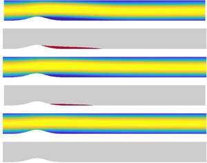
The above analysis was extended to include slip (2.4) along the bump region,  $\varGamma _2$. The main qualitative conclusion that can be drawn from our analysis is that slip can be used to delay the onset of separation and reduce the intensity of the separation bubble that forms along the rear side of the bump. This observation is demonstrated in figures 5 and 6, which display contours of the streamwise velocity for two representative Reynolds numbers, ${\textit {Re}}=2000$ and ${\textit {Re}}=4000$. In each instance, the slip length $\lambda$ is increased from zero to $0.2$ monotonically down the figure in intervals of $\Delta \lambda =0.04$. All contour plots for ${\textit {Re}}=2000$ are plotted at non-dimensional time $t=100$, which was again sufficient to achieve a steady state. For the larger Reynolds number, ${\textit {Re}}=4000$, it was necessary to extend DNS computations to larger time, with a steady state eventually realised at $t=200$. Moreover, simulation results for the two Reynolds numbers are presented for the same slip lengths, to facilitate comparison of the effect of slip on flow separation. As in figure 3, yellow and blue contours are matched to the respective streamwise velocities $u=1$ and $u\leqslant 0$, while the secondary plots highlight the regions, in red, of recirculation (that is, where $u<0$).

Figure 5. Contour plots of the streamwise  $u$-velocity for the Reynolds number ${\textit {Re}}=2000$ and slip length (a) $\lambda =0$, (b) $\lambda =0.04$, (c) $\lambda =0.08$, (d) $\lambda =0.12$, (e) $\lambda =0.16$ and (f) $\lambda =0.2$. Secondary plots highlight the regions of separation, in red, where $u<0$.

Figure 6. Same as figure 5, but for the Reynolds number  ${\textit {Re}}=4000$ and non-dimensional time $t=200$. (a) $\lambda = 0$, (b) $\lambda = 0.04$, (c) $\lambda = 0.08$, (d) $\lambda = 0.12$, (e) $\lambda = 0.16$ and (f) $\lambda = 0.2$.
As the slip length  $\lambda$ increases, the onset of separation along the rear side of the bump is delayed, that is, the streamwise location $x_s$ moves downstream. Additionally, the streamwise location $x_r$ at which the flow reattaches is generally found to move upstream. (There are a few exceptions to this, for the Reynolds number ${\textit {Re}}=4000$ and small slip lengths $\lambda$. This particular flow characteristic will be discussed in greater detail below.) Thus, the length of the separation bubble, behind the bump, decreases as the slip length $\lambda$ increases. Moreover, the ‘thickness’ of the separation bubble diminishes as $\lambda$ increases. This behaviour is qualitatively equivalent for both Reynolds numbers ${\textit {Re}}$ under consideration, although for a fixed slip length $\lambda$, flow reattachment is always found at larger streamwise locations for ${\textit {Re}}=4000$, as one would anticipate on the basis of the analysis of Smith (Reference Smith1976) for the full no-slip case. Eventually, the streamwise locations for the onset of separation $x_s$ and reattachment $x_r$ coalesce and the flow no longer separates. For those parameters considered in figures 5 and 6, separation does not occur for a slip length $\lambda =0.2$.
Velocity profiles of the streamwise  $u$-velocity are plotted in figure 7 for three fixed streamwise $x$-positions: the bump centre ( $x=0$); the recirculating region ( $x=4$); and far downstream of the separation bubble ( $x=19$). Results are plotted for slip lengths $\lambda =0$ (solid line), $\lambda =0.08$ (dashed) and $\lambda =0.16$ (chain), with plots on the upper row matched to the Reynolds number ${\textit {Re}}=2000$ and those on the lower row to ${\textit {Re}}=4000$. In addition, each solution has been scaled to have a maximum value of unity; the emergence of flow separation and the application of slip to the lower channel surface brings about a small increase in the $u$-velocity maximum. In figures 7(a) and 7(d) (that correspond to $x=0$), the application of no-slip along the bump region can be seen to establish a sharp change in the $u$-velocity field near the lower channel wall (solid lines), while slip induces a non-zero velocity at the bump tip (dashed and chain lines). Moreover, the bump has shifted the maximum $u$-velocity downwards towards the lower channel wall. At the streamwise position $x=4$, plotted in figures 7(b) and 7(e), the $u$-velocity at the lower wall is zero in each instance; this particular location is found in region $\varGamma _3$ that is downstream of the slip region $\varGamma _2$. From figures 7(b) and 7(e) the thickness of the separation bubble that forms on the rear side of the bump can be estimated. For the case without slip, the $u$-velocity is negative for $y \leqslant 0.2$ and $y \leqslant 0.3$, for the respective Reynolds numbers ${\textit {Re}}=2000$ and ${\textit {Re}}=4000$. Hence, the region of separation thickens as the Reynolds number increases. Furthermore, the application of slip to the bump region reduces the thickness of the separation bubble. At the downstream location, $x=19$, the flow recovers behaviour consistent with the typical parabolic profile of fully developed plane-Poiseuille flow, as can be seen in figures 7(c) and 7(f). We note that there remains a small downwards shift in the maximum velocity, especially in the case of no-slip. This is a direct consequence of the flow requiring a greater streamwise domain to adjust to the pocket of separated flow. Eventually, for large enough $x$, the flow will evolve to fully developed plane-Poiseuille flow.

Figure 7. Streamwise  $u$-velocity profiles (normalised on the local maximum) are plotted for slip lengths $\lambda = 0$ (solid lines), $\lambda = 0.08$ (dashed) and $\lambda = 0.16$ (chain), for the Reynolds number (a–c) ${\textit {Re}}=2000$ and (d–f) ${\textit {Re}}=4000$, at the streamwise locations $x= 0$, $x = 4$ and $x = 19$, respectively. Results are plotted at non-dimensional time $t=100$ and $t=200$ for ${\textit {Re}}=2000$ and ${\textit {Re}}=4000$, respectively.
The effects of the slip length  $\lambda$ and Reynolds number ${\textit {Re}}$ on the size of the separation bubble that forms along the rear side of the bump, are further illustrated in figure 8. Streamlines of the steady flow are plotted for slip lengths $\lambda = 0$ (no-slip), $\lambda =0.06$, $\lambda =0.12$ and $\lambda =0.18$. Within each subplot, solutions are displayed for both Reynolds numbers, ${\textit {Re}}=2000$ and ${\textit {Re}}=4000$. As noted above, the recirculation region is longer and thicker for the larger Reynolds number. Additionally, the significant influence of slip is evident in both cases, establishing both a delay in the onset of separation and a shortening of the bubble's length. However, for ${\textit {Re}}=4000$, a larger slip length $\lambda$ is always necessary to reduce the streamwise length of the recirculation region; separation is suppressed by setting $\lambda =0.18$ in the instance ${\textit {Re}}=2000$, while a small region of recirculation is found in the streamwise interval $2 < x < 4$ for ${\textit {Re}}=4000$. However, as shown in figure 6(f), this disappears for $\lambda =0.2$.

Figure 8. Streamlines of the steady flow in the region of the bump, obtained at non-dimensional time  $t = 100$ and $t=200$ for the respective Reynolds numbers ${\textit {Re}}=2000$ and ${\textit {Re}}=4000$. The slip length (a) $\lambda = 0$, (b) $\lambda = 0.06$, (c) $\lambda = 0.12$ and (d) $\lambda = 0.18$.
The non-dimensional shear stress at the wall
 \begin{equation} \tau_w=\left.\dfrac{\partial u}{\partial y}\right|_{y=0}, \end{equation}
is plotted in figure 9 for slip lengths  $\lambda =0$ (solid lines), $\lambda =0.1$ (dashed) and $\lambda =0.2$ (chain). Results in figure 9(a) are for a Reynolds number ${\textit {Re}}=2000$, while those in figure 9(b) correspond to ${\textit {Re}}=4000$. For both Reynolds numbers under consideration, the wall shear stress $\tau _w$ increases along the front side of the bump, before decreasing sharply along the rear side. This behaviour is more pronounced for the larger Reynolds number. When the slip length $\lambda =0$ (the classical no-slip case), a negative valued $\tau _w$ is realised that extends a significant streamwise length downstream until flow reattachment occurs (which is consistent with that presented above in figures 5–8). Downstream of the reattachment location, the wall shear stress $\tau _w$ approaches a value of $2$, which is consistent with that expected of the fully undisturbed plane-Poiseuille flow in this region (2.6). The application of slip to the bump surface significantly reduces both the increase and decrease in the wall shear stress $\tau _w$ along the respective front and rear sides of the bump. Indeed, when the slip length $\lambda =0.2$, $\tau _w>0$ for all streamwise $x$-positions.

Figure 9. Wall shear stress,  $\tau _w$, for the Reynolds numbers (a) ${\textit {Re}}=2000$ at $t=100$, (b) ${\textit {Re}}=4000$ at $t=200$. The slip length $\lambda =0$ (solid lines), $\lambda =0.1$ (dashed) and $\lambda =0.2$ (chain). The insert plots depict the area of the separated region $A_{\tau _w}$, as given by (3.2), as a function of the slip length $\lambda$.
The insert plots in figure 9(a) and 9 (b) illustrate how the area of the separated region
 \begin{equation} A_{\tau_w} = \left| \int_{x_s}^{x_r} \tau_w(x) \, \textrm{d}\kern0.7pt x \right|, \end{equation}
varies in relation to the slip length  $\lambda$, for the Reynolds numbers ${\textit {Re}}=2000$ and ${\textit {Re}}=4000$. For the no-slip case ( $\lambda =0$), the area of the separated region $A_{\tau _w} \approx 7$ when ${\textit {Re}}=2000$, whereas for ${\textit {Re}}=4000$ the area $A_{\tau _w} \approx 13$. The area of the separated region $A_{\tau _w}$ is approximately halved when the slip length $\lambda =0.08$, while $A_{\tau _w}$ is equal to zero in both cases (i.e. no separated flow), for $\lambda =0.2$.
The intensity of the recirculation region, on the rear side of the bump, can be quantified by computing the absolute value of the minimum of the streamwise  $u$-velocity, $\| \min (u) \|$. In figure 10, $\| \min (u) \|$ is plotted as a function of the slip length $\lambda$, for both Reynolds numbers ${\textit {Re}}=2000$ and ${\textit {Re}}=4000$. In addition, results are shown at several points in time, providing a further demonstration of the flow evolution, and confirmation that a steady state is achieved for sufficiently large time. Convergence to a steady state is realised by non-dimensional time $t=60$ for ${\textit {Re}}=2000$ and $t=160$ for ${\textit {Re}}=4000$, respectively. Additionally, for suitably large time, $\| \min (u) \|$ is found to decrease linearly with the slip length $\lambda$, with no separation bubble forming behind the bump for $\lambda \geqslant 0.18$ and $\lambda \geqslant 0.2$ for the respective Reynolds numbers ${\textit {Re}}=2000$ and ${\textit {Re}}=4000$. Furthermore, the intensity of the separation bubble is greater for the larger Reynolds number, especially during the initial stages of the numerical simulation.

Figure 10. Plots of the absolute value of the minimum of the streamwise  $u$-velocity, $\|\min (u)\|$, found within the separation bubble on the rear side of the bump, as a function of the slip length $\lambda$. (a) ${\textit {Re}} = 2000$ and (b) ${\textit {Re}} = 4000$.
In figure 11(a) we present plots of the position of the onset of separation, which can readily be seen to shift along the right-hand side of the bump as slip increases. The onset occurs earlier in space for  $\lambda = 0$ and $0.04$ when ${\textit {Re}}=4000$, almost at the same position for both Reynolds numbers for $\lambda =0.08$ and $0.12$, and slightly earlier for $\lambda =0.16$ at ${\textit {Re}}=4000$.

Figure 11. Plots of (a) the position  $x_s$ for the onset of separation and (b) the absolute value of the bubble length $\mathcal {L}_x$ versus the slip length $\lambda$. Results are shown at $t=100$ for ${\textit {Re}}=2000$ and $t=200$ for ${\textit {Re}}=4000$.
To quantify the length of the separation bubble, we define  $\mathcal {L}_x$ as the length of the separation bubble measured along the $x$-axis, such that $\mathcal {L}_x = x_r - x_s$. In figure 11(b), the variation of $\mathcal {L}_x$ with the slip length $\lambda$ is shown. The length of the separation bubble is larger for the higher Reynolds number and, in both cases, $\mathcal {L}_x$ decreases to zero as slip increases, with critical values of $\lambda =0.18$ for ${\textit {Re}} = 2000$ and $\lambda =0.2$ for ${\textit {Re}}=4000$. Interestingly, we also note from figure 11 that for the higher Reynolds number case, slip does not have a monotonic effect upon the length of the separation bubble, only showing clear signs of a decrease when $\lambda$ is above $0.06$. We conjecture that this particular feature may be due to the fact that, for a higher Reynolds number where the intensity of separation is enhanced, a moderate slip length (that is, $\lambda < 0.06$) is not sufficient to counteract the reversed flow. Thus, only for $\lambda >0.06$ does the beneficial effect of slip become evident.
3.1. Skin-friction and pressure drag coefficients
Skin-friction and pressure at the wall are defined locally by the non-dimensional coefficients
 \begin{equation} c_f(x) = \dfrac{2\tau_w^*(x)}{\rho^* U_m^{*2}} \quad \textrm{and} \quad c_p(x) =\dfrac{2 p^* (x)}{\rho^* U_m^{*2}}, \end{equation}
(Banchetti, Luchini & Quadrio Reference Banchetti, Luchini and Quadrio2020). Using the length  $h^*$, velocity $U_m^*$ and pressure $\rho ^*U_m^{2*}$ scales, the skin-friction and pressure coefficients are recast as
 \begin{equation} c_f(x) = \dfrac{2 }{{\textit{Re}}} \tau_w (x) \quad \textrm{and} \quad c_p(x) = 2 p (x), \end{equation}
where  $\tau _w (x)$ denotes the non-dimensional shear stress at the wall given by (3.1). Effectively, the skin-friction coefficient $c_f(x)$ is the wall-shear stress $\tau _w (x)$ plotted in figure 9, scaled by the factor $2/{\textit {Re}}$.
In order to demonstrate the effect of slip on the pressure field over the bump, the pressure distribution  $p$ is plotted in figure 12, for the Reynolds number ${\textit {Re}}=2000$ and slip lengths $\lambda =0$, $\lambda =0.08$ and $\lambda =0.16$. Pressure decreases as the flow passes from left to right over the bump, with a local minimum found shortly after the bump tip due to the negative wall curvature. For those slip cases shown, the local maximum found on the leeward side of the bump decreases, while the local minimum located about the bump tip shows clear signs of a reduced intensity; lighter blue contours.

Figure 12. Contour plots of the pressure  $p$ in the $(x,y)$-plane, for the Reynolds number ${\textit {Re}}=2000$, and slip lengths (a) $\lambda =0$, (b) $\lambda =0.08$ and (c) $\lambda =0.16$. Thick dashed black lines indicate $p = 0$.
The skin-friction and pressure contributions to the total drag are defined by Mollicone et al. (Reference Mollicone, Battista, Gualtieri and Casciola2017) as
 \begin{equation} C_f = \frac{1}{L_x} \int_{\varOmega_{\bar{x}} } c_f(x) \,\textrm{d}\kern0.7pt x \quad \textrm{and} \quad C_p ={-} \frac{1}{L_x} \int_{\varOmega_{\bar{x}}} c_p(x) \boldsymbol{i} \boldsymbol{\cdot} \boldsymbol{n} \,\textrm{d}\kern0.7pt x, \end{equation}
where  $L_x$ denotes the streamwise length of the computational domain $\varOmega _{\bar {x}}$, $\boldsymbol {i}$ represents the unit vector in the streamwise $x$-direction and $\boldsymbol {n}$ again denotes the unit normal vector that points into the fluid domain. In (3.5b), the scalar product $\boldsymbol {i} \boldsymbol {\cdot } \boldsymbol {n} \neq 0$ along the bump surface and zero elsewhere. Thus, the contribution of the pressure drag $C_p$ to the total drag comes only from the pressure acting on the bump wall.
The respective percentage reductions in the skin-friction drag  $C_f$ and pressure drag $C_p$ are computed using the formulae
 \begin{equation} \mathcal{R}_{C_f} (\%) = 100 \left(1- \dfrac{C_{f,\lambda}}{C_{f,0}} \right) \quad \textrm{and} \quad \mathcal{R}_{C_p} (\%) = 100 \left( 1- \dfrac{ C_{p,\lambda}}{C_{p,0}} \right), \end{equation}
where  $C_{f,\lambda }$ and $C_{p,\lambda }$ represent the respective skin-friction and pressure components of drag in the instance slip (with slip length $\lambda$) is applied to the bump surface. Skin-friction and pressure drag components, $C_{f,0}$ and $C_{p,0}$, then denote the reference case in which no-slip (that is, $\lambda =0$) is applied along the channel walls.
Total drag is defined as the sum of the skin-friction drag and pressure drag:
 \begin{equation} \mathcal{D}_{\lambda} = C_{f,\lambda} + C_{p,\lambda}. \end{equation}
Therefore, the total percentage drag reduction is obtained via the formula
 \begin{equation} \mathcal{R}_{\mathcal{D}} (\%) = 100 \left(1- \dfrac{\mathcal{D}_{\lambda}}{\mathcal{D}_0} \right), \end{equation}
where  $\mathcal {D}_0=C_{f,0} + C_{p,0}$.
The total percentage drag reduction is plotted in figure 13 as a function of the slip length  $\lambda$ (yellow squares), together with the corresponding percentage reductions in the skin-friction drag (blue circles) and pressure drag (red diamonds), for the Reynolds numbers ${\textit {Re}}=2000$ and ${\textit {Re}}=4000$. A peak percentage reduction in the skin-friction drag is achieved in both instances for a slip length $\lambda \approx 0.08$, while the percentage reduction in the pressure drag increases almost linearly with $\lambda$. Overall, the total percentage drag reduction increases with an increasing slip length $\lambda$, with $27\,\%$ and $35\,\%$ total drag reductions achieved in the instance the slip length $\lambda =0.2$, for ${\textit {Re}}=2000$ and ${\textit {Re}}=4000$, respectively.

Figure 13. Skin-friction (blue circles), pressure (red diamonds) and total (yellow squares) percentage drag reduction as a function of the slip length  $\lambda$, for the Reynolds numbers (a) ${\textit {Re}}=2000$ and (b) ${\textit {Re}}=4000$.
3.2. Effect of slip applied across the entire lower wall
The question of why we have chosen to apply slip along a specific streamwise region rather than across the full length of the lower surface is an obvious one. From the perspective of industrial applications, such as surface coatings, the implications of covering an entire surface versus a targeted area can have a substantial impact on economic costs. Therefore, if it is possible to achieve the same laminar flow control benefits at a reduced expense, it is generally advisable to do so. In the following, we compare the benefits of applying slip across the entire lower wall,  $\varGamma$, with that realised when slip is limited to the bump region, $\varGamma _2$.
Slip is applied across the full length of the lower wall,  $\varGamma$, by recasting the coupled linear Robin-type slip boundary condition and no-penetration condition (2.4) as
 \begin{equation} u - \lambda \frac{\partial u}{\partial n} =0 \quad \textrm{and} \quad v = 0, \end{equation}
where the slip length  $\lambda$ is constant and $n$ again denotes the direction normal to the lower wall. As before, all results are independent of the mesh used.
A quantitative analysis of the two approaches to slip application is reported in table 2. Here the minimum value of the streamwise  $u$-velocity within the separation bubble, $\min (u)$, is tabulated, for Reynolds numbers ${\textit {Re}} = 2000$ and $4000$, at the respective times $t=100$ and $t=200$, that is, those points in time that a steady state has been realised. (Subscripts $\varGamma$ and $\varGamma _2$ represent the application of slip to the full lower surface and to the bump region.) Moreover, calculations are presented for four slip lengths $\lambda \in [0.05,0.2]$. In general, $\min (u)$ is reduced when slip is applied across the entire lower wall, that is, the intensity of the separation bubble decreases. Additionally, flow separation is inhibited (that is, $\min (u) = 0$) at smaller values of the slip length $\lambda$ when slip is applied across the full length of the lower surface; $\lambda = 0.15$ is sufficient to stop the flow separating for both Reynolds numbers under consideration, while marginally larger slip lengths are necessary to suppress flow separation when slip is limited to the bump region.
Table 2. Minimum value of the streamwise  $u$-velocity, $\min (u)$, obtained for Reynolds numbers ${\textit {Re}}=2000$ and $4000$, at times $t=100$ and $200$, respectively. Subscripts $\varGamma$ and $\varGamma _2$ represent the application of slip to the entire lower surface and to the bump region.

In conclusion, applying slip across the full length of the lower wall inhibits the emergence of flow separation at smaller slip lengths  $\lambda$, but the qualitative effect of slip on the flow separation dynamics is equivalent for both methods.
4. Concluding remarks
In this work, DNS have been performed to study the influence of a Robin-type slip boundary condition on the dynamics of the two-dimensional wake occurring behind a Gaussian-shaped bump in a channel. Specifically, it has been shown that surface slip: (i) decreases the intensity of the separation, (ii) delays, and ultimately inhibits, the onset of recirculation and in doing so (iii) reduces the dimensions of the separation bubble. There are a number of ways in which this work could be extended. One could vary the aspect ratio  $\eta$ and conduct a systematic study to investigate the effect of the bump's height in relation to different Reynolds numbers and slip lengths. (A brief summary of the effect of slip on other bump configurations is presented in the Appendix.) Alternatively, one could vary the length of the slip region $\varGamma _2$ along the lower wall and study the dynamics of the flow as a function of the dimensions of the slip region. Another direction would be to modify the type of application of slip on the bump. Slip is now applied in a Gaussian fashion to allow a smooth transition between the slip and no-slip region. This approach could be modified to determine a, possibly more efficient, way of introducing slip on a curved surface. Furthermore, one could extend the problem in three-dimensions, either in full three-dimensional (3-D) or quasi-3-D using a Fourier expansion in the span direction (Karniadakis Reference Karniadakis1990), and investigate the effect of slip applied both in the streamwise and spanwise directions on a fully 3-D bump.
Declaration of interests
The authors report no conflict of interest.
Appendix. Effect of slip on different bump configurations
The above analysis was performed on the two-dimensional flow that develops in a channel over a bump of fixed aspect ratio  $\eta =0.5$ (that is, an amplitude $A=1/\eta =2$), for the Reynolds numbers ${\textit {Re}}=2000$ and ${\textit {Re}}=4000$. This bump configuration and flow conditions were chosen as they were sufficient to establish a well-defined separation bubble on the rear side of the bump in the instance no-slip was applied to the channel walls. Hence, these particular parameter values were suitable for demonstrating the control benefits brought about by the application of slip to the bump surface. However, further bump configurations were modelled that illustrate comparable control of flow separation due to the application of slip. Table 3 presents the minimum value of the streamwise $u$-velocity, $\min (u)$, obtained for several bump-flow configurations characterised by the aspect ratio $\eta$, Reynolds number ${\textit {Re}}$ and slip length $\lambda$. The slip lengths labelled $\lambda ^{\star }$ correspond to those parameters discussed at length in this paper, and were included here for reference.
Table 3. Minimum value of the streamwise  $u$-velocity, $\min (u)$, obtained for different bump-slip configurations characterised by the slip length $\lambda$, aspect ratio $\eta$ and Reynolds number ${\textit {Re}}$. Here $^{\star }$ indicates those results presented in the main body of this paper.

Results presented in the first two columns of table 3 correspond to those Reynolds number modelled throughout this study (that is,  ${\textit {Re}}=2000$ and ${\textit {Re}}=4000$). Two additional results are included in the first column that are matched to larger bumps, with the aspect ratio $\eta =0.48$ and $\eta =0.47$, respectively. In both instances, flow separation is inhibited by the application of slip with the slip length $\lambda =0.2$ (i.e. the same as that found for $\eta =0.5$).
The right-hand column of table 3 presents results corresponding to the Reynolds number  ${Re}=5000$. (Note that $y^+ \approx 0.7$ for ${Re}=5000$.) When no-slip is applied to the same bump geometry modelled throughout this paper (i.e. $\eta =0.5$), the minimum value of the streamwise $u$-velocity, $\min (u)$, is greater for ${Re}=5000$ compared with those calculations obtained for the two smaller valued Reynolds numbers. Nevertheless, slip is again found to bring about favourable control benefits, with slip attenuating the intensity of the recirculation region and $\min (u)$ decreasing as the slip length $\lambda$ increases. For smaller bump configurations, the flow does not separate under any circumstances (including no-slip) when the aspect ratio $\eta =2$, whereas for $\eta =1$ flow separation is inhibited for a small slip length $\lambda =0.1$.


 Open access