

1. Introduction
The global land ice mass is equivalent to ∼65 m rise of the mean global sea level (AMAP, 2011), but only 1% is stored in glaciers outside the Greenland and Antarctic ice sheets. Nevertheless, glaciers have contributed about one-third of the observed sea-level rise over the past 50 years (Reference ChurchChurch and others, 2011) and are expected to remain an important component, at least for the 21st century (Reference MeierMeier and others, 2007; Reference Radic and HockRadic and Hock, 2011). The release of water from glacier storage is accomplished by iceberg calving and meltwater runoff. The rate of meltwater production is primarily dictated by the receipts of energy from the atmosphere at the glacier surface. A significant part of this meltwater may be retained by refreezing in the glacier as a consequence of low ice temperatures, especially in Arctic polythermal glaciers (e.g. Reference Pfeffer, Meier and IllangasekarePfeffer and others, 1991). The Arctic has experienced pronounced warming since the 1970s, with highest warming rates in the winter (e.g. AMAP, 2011). The retention capacity due to refreezing is also controlled by winter climate (Reference Bøggild, Forsberg and ReehBøggild and others, 2005). Projections of future climate indicate continued warming above the global average (e.g. AMAP, 2011), and a potential reduction of the refreezing capacity may further enhance mass loss from Arctic glaciers (Reference Wright, Wadham, Siegert, Luckman and KohlerWright and others, 2005). Global estimates for mass balance of glaciers over the 21st century typically treat refreezing in a simple manner. For instance, Reference Giesen and OerlemansGiesen and Oerlemans (2012) treat refreezing with a simple physical model, while Reference Radic and HockRadic and Hock (2011) relate mean annual air temperature to refreezing, following Reference Woodward, Sharp and ArendtWoodward and others (1997). Several studies have evaluated the usefulness of different parameterizations (Reference Wright, Wadham, Siegert, Luckman, Kohler and NuttallWright and others, 2007; Reference Reijmer, Van den Broeke, Fettweis, Ettema and StapReijmer and others, 2012). In general, most parameterizations perform satisfactorily when carefully calibrated; however, the transferability of such parameterizations to other regions or different climate conditions is questionable (Reference MacDougall, Wheler and FlowersMacDougall and others, 2011).
In this paper, our aim is to quantify the components of the surface energy balance, with special emphasis on the subsurface heat exchange at Austfonna, an Arctic ice cap in the Svalbard archipelago. A coupled energy-balance and snowpack model (Reference Hock and HolmgrenHock and Holmgren, 2005; Reference Reijmer and HockReijmer and Hock, 2008) is applied to the site of an automatic weather station (AWS) over five consecutive melt seasons (2004–08). A Monte Carlo approach is adopted to determine values for some of the less-constrained parameters within their ranges of physically plausible values. In addition, evaluating the ensemble of realizations using a multiple-criteria scheme allows an assessment of the parametric uncertainty (e.g. Reference Fitzgerald, Bamber, Ridley and RougierFitzgerald and others, 2012; Reference Rye, Willis, Arnold and KohlerRye and others, 2012). Finally, we discuss the importance of subsurface heat exchange for glacier mass balance.
2. Study Site and Field Measurements
Located between the northern tip of the North Atlantic current and the southern edge of the multi-year sea ice, the Arctic archipelago Svalbard is one of the most climatically sensitive regions of the world (Reference Rogers, Yang and LiRogers and others, 2005). Both temperature and precipitation have large interannual variability, depending on the cyclone activity (Reference Hanssen-Bauer and FørlandHanssen-Bauer and Førland, 1998). Winters are relatively mild, despite the northern latitude; air temperature rarely drops below — 40°C and short melt events and rainfall are not uncommon in midwinter (Reference NordliNordli, 2010). Over the period 2004-11 the mean annual air temperature at the automatic weather station AWS-1 on the Austfonna ice cap (Fig. 1) was —8.5°C, while the winter mass balance was typically 0.3-0.4 m w.e. a∼1 and the summer mass balance —0.2 to — 1.1 m w.e. a - 1 .
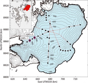
Fig. 1. Overview map showing Austfonna in the northeast of Svalbard (inset). Lines indicate the transects along which annual field surveys have been conducted since 2004, dots indicate locations of mass-balance stakes. AWS-1 (369ma.s.l.) and AWS-2 (537 m a.s.l.) give the locations of two automatic weather stations. Contours with 50m spacing.
Austfonna is a large polythermal ice cap centered at 80° N, 24° E in northeastern Svalbard in the Norwegian Arctic (Fig. 1). The ice cap has a simple dome-shaped geometry and covers an area of ∼-7800km2, with altitude ranging from sea level up to 800 m a.s.l. (Reference Moholdt and KaabMoholdt and Kaab, 2012). In the south and east, the ice cap is grounded below sea level, while in the north and west it mostly terminates on land, except where it flows into several narrow fjords (Reference Dowdeswell, Drewry, Cooper, Gorman, Liestøl and OrheimDowdeswell and others, 1986). The melt period is usually limited to a few weeks between mid-June and the end of August, often interrupted by cold spells and snowfall events (Reference Schuler, Loe, Taurisano, Eiken, Hagen and KohlerSchuler and others, 2007; Reference Rotschky, Schuler, Haarpaintner, Kohler and IsakssonRotschky and others, 2011).
In 2004 a network of ∼20 mass-balance stakes was established, and it has been maintained every spring since then (Reference Moholdt, Hagen, Eiken and SchulerMoholdt and others, 2010). Since 2004, two AWSs have operated at 369 and 537 m a.s.l., referred to as AWS-1 and AWS-2, respectively (Fig. 1). Both stations measure air temperature, relative humidity, wind speed, wind direction and vertical surface displacement, using a sonic ranger mounted on a stake drilled into the ice; AWS-1 additionally records the four radiation components, shortwave incoming and reflected radiation and longwave incoming and outgoing radiation (Table 1). Next to AWS-1, snow and ice temperatures are measured at eight to ten depth levels from the surface to 10m depth. In addition, at both AWSs, traditional mass-balance measurements, based on stake readings and snow density profiles in snow pits, are performed. Mean snow density is ∼390kgmr3 , with low spatial and interannual variability. Each spring, the snow distribution has been mapped along several ground-penetrating radar profiles (Fig. 1) (Reference Dunse, Schuler, Hagen, Eiken, Brandt and HøgdaDunse and others, 2009). The distribution of snow across the ice cap displays a dominating southeast-northwest trend of snow depth, typically ∼2.5 m in the southeast and decreasing to <1 m in the northwest (Reference TaurisanoTaurisano and others, 2007; Reference Dunse, Schuler, Hagen, Eiken, Brandt and HøgdaDunse and others, 2009). This horizontal gradient reflects the precipitation pattern resulting from moisture advection from the Barents Sea, with southeasterly airflow (Reference Førland, Hanssen-Bauer and NordliFørland and others, 1997). Between 2004 and 2008, Austfonna experienced a gradual expansion of its firn area (Reference Dunse, Schuler, Hagen, Eiken, Brandt and HøgdaDunse and others, 2009). The site of AWS-1 was originally (2004) located in the ablation area, but being persistently covered by snow in 2008, it became part of the accumulation area.
Table 1. Overview of measurements, along with sensor type and associated factory uncertainty, recorded at AWS-1 and at AWS-2. Hourly means are obtained by measuring every second minute for radiation, wind and surface displacement, and every sixth minute for temperature and humidity
3. Model Description
A coupled surface energy balance and snowpack model is used to calculate surface energy fluxes, mass balance, water retention and snow and ice properties. The model is described in detail by Reference Reijmer and HockReijmer and Hock (2008) and Reference Hock and HolmgrenHock and Holmgren (2005).
3.1. Surface energy balance
The energy balance describes all fluxes of energy directed towards or away from a considered surface. The sign convention is that energy fluxes towards the surface are positive and those directed away from the surface are negative (e.g. Reference HockHock, 2005). The energy balance is computed as
where S| is incoming solar radiation, a is albedo, L| and Li-are incoming and outgoing longwave radiation, H and E are the turbulent fluxes of sensible heat and latent heat, R is energy flux supplied by rain, G is energy exchange with subsurface volume and M is latent energy flux related to melting.
Here we take the incoming solar radiation, albedo and incoming longwave radiation from measurements. Surface temperature and emitted longwave radiation are calculated by the model to ensure consistency with subsurface temperatures. Emitted longwave radiation is derived from the surface temperature using the Stefan-Boltzmann law,
where e = 1 is the emissivity, a = 5:670 x 10T8Wmr2 K∼4 the Stefan-Boltzmann constant and Ts the surface temperature calculated by the snowpack model. The turbulent fluxes of sensible heat, H, and latent heat, E, are calculated according to the Monin-Obukhov similarity theory (as described by Reference Hock and HolmgrenHock and Holmgren, 2005), using measurements of air temperature and relative humidity at a single level. At the surface level, we assume the presence of a moisture-saturated (RH (relative humidity) = 100%) boundary layer, the moisture content of which depends on temperature. Roughness lengths of momentum, heat and moisture are assumed to be equal, but different for snow and ice. Values for the roughness lengths of snow and ice are assigned during the calibration process (Section 4.3).
Rainwater temperature is assumed to be equal to the air temperature, and the rain energy flux, R, is taken to be the product of the rainfall rate and the specific heat capacity of water, cw = 4180J K∼1 kg∼1.
3.2. Snowpack routine
The snowpack routine calculates the ground heat flux, G, the surface temperature, Ts, the energy consumed or produced by melt and refreezing, M, and considers the associated evolution of snow density. The model is based on the snowpack model SOMARS (Simulation Of glacier surface Mass balance And Related Sub-surface processes), developed by Reference Greuell and KonzelmannGreuell and Konzelmann (1994) and modified by Reference Reijmer and HockReijmer and Hock (2008). Snow and ice temperature, density and water content are calculated on an adaptive grid consisting of 15-30 vertical grid layers 5 cm thick close to the surface, and up to 5 m thick layers at the maximum model depth, ∼33 m. The model creates, splits and merges layers: in the case of snowfall a new layer is created, if the layers are too thick they are split, or if a layer is <2.5cm thick it is merged with the layer below. Horizontal fluxes of any properties are not considered.
The evolution of the subsurface temperature is calculated by solving the thermodynamical equation explicitly on the subsurface grid:
where the specific heat capacity of ice is considered constant, cpi = 2009J kg∼1 K∼1, T = T(z, t) is temperature, z and t represent the depth below surface and time, respectively, and K is the density-dependent effective thermal conductivity, which implicitly accounts for penetration of solar radiation. (See Section 4.3 for more information on the conductivity parameterization.) Q represents a production term which is given by
At the surface, Q(z = 0) represents energy exchange with the atmosphere. When neither melting nor refreezing occurs, Q = S|(1 — a) + Li + Li + H + E + R. Below the surface (z > 0), Q accounts for consumption or release of latent heat associated with melting and refreezing, respectively. Occurrence of subsurface temperatures above the melting point is inhibited by capping T at 0°C and devoting excess energy to melt in the current layer. When melting occurs, the meltwater is added to the water content of the considered layer; at the surface, the rainfall volume rate, R=(Lf Pw), is additionally considered; here Lf = 0:335 x 106 J kg∼1 is the latent heat of fusion and pw = 1000 kg m r 3 the density of water. In the presence of liquid water at T < 0, refreezing occurs and M < 0 represents the associated release of latent energy.
As such, refreezing depends on temperature and availability of pore space and water. Once the cold content is eliminated, further meltwater follows gravity and percolates towards deeper layers, but a small amount of water is retained by capillary forces. This irreducible water content is a function of density and is described using a relationship by Reference Schneider and JanssonSchneider and Jansson (2004). Ice is considered impermeable and hence forms a barrier for percolation. Above an ice layer, water can accumulate and form a slush layer. Runoff occurs from the slush layer and is calculated using a relationship proposed by Reference Zuo and OerlemansZuo and Oerlemans (1996),
where the coefficients c1, c2 and c3 are runoff timescales for different slopes, which are used to calculate the overall runoff timescale as a function of surface slope, /3 (see Reference Reijmer and HockReijmer and Hock, 2008, for details). c 0 is a coefficient to delay runoff in the snowpack compared to that at the surface, so c 0 = 0 when the slush height reaches the total snow depth (see Section 4.3 for runoff coefficient values). In addition to density changes caused by percolation and melt/ refreezing, the density of dry snow changes as a function of temperature and accumulation rate, following the parameterization of Reference Li and ZwallyLi and Zwally (2004), based on Reference Herron and LangwayHerron and Langway (1980). Precipitation is added in the uppermost layer of the model. In the case of rain, the water content is successively raised and in the case of snowfall more mass is added and a new layer created if necessary. Note that refreezing includes all refrozen water in any layer of the snowpack model, whether it is in the snow or on top of the last summer surface (from the slush layer) known as superimposed ice.
Solution of Eqn (3) requires prescription of boundary conditions. At the surface Q(z = 0) is used as a Neumann boundary condition, and at the bottom of the deepest model layer (z ∼ 33 m) we assume zero heat flux (dT=dz = 0).
4. Model Application
The model is applied to the location of AWS-1 over the five melt seasons 2004-08. For each melt season, simulations are performed from the end of April (more specifically, the date when AWS-1 was visited) until the beginning of October. The surface energy balance was calculated at time-steps of 1 hour, whereas the snowpack model was executed at ten sub-intervals within each hour.
4.1. Meteorological forcing
Hourly measurements of air temperature, wind speed, relative humidity, surface displacement and three of the radiation components (S|, Si used for a, and Ly) were used as model input and to evaluate model performance. Instrument failure caused interruptions of the temperature and humidity records during the 2007 and 2008 melt seasons. Data gaps at AWS-1 were filled using adjusted data from AWS-2 (Fig. 1) when 4 months of air temperature were missing in 2007 and when 2 months of air temperature and relative humidity were missing in 2008. The gaps were filled using a melt season temperature lapse rate of 4.58Ckm∼1, the observed 2004-07 average. The high correlation between RH measured at AWS-1 and AWS-2 (r2 = 0:77) was exploited to fill the gaps in the RH record. Occasionally the reflected shortwave radiation far exceeded the incoming shortwave radiation, and comparison with the surface displacement record revealed that these situations coincided with snowfall events, presumably leading to coverage of the upward-looking sensor. In such cases, incoming shortwave radiation was determined by multiplying the reflected shortwave radiation by 1.1, representing an albedo of 0.91 during snowfall.
Precipitation for the location of AWS-1 is derived from the ERA-Interim reanalysis of the European Centre for Medium-Range Weather Forecasts (Reference DeeDee and others, 2011), using a linear theory of orographic precipitation enhancement (Reference Smith and BarstadSmith and Barstad, 2004). Based on wind direction, speed and temperature from the ERA-Interim reanalysis, the orographic enhancement was calculated and superimposed on the ERA-Interim precipitation at a spatial resolution of 1 km and time-steps of 6 hours. To comply with the underlying assumption of moisture-saturated air, the procedure was applied only when ERA-Interim reanalysis predicted RH > 90%. The method has previously proved valuable for downscaling precipitation for glaciological applications (Reference Crochet, Jóhannesson and JonssonCrochet and others, 2007; Reference Schuler, Crochet, Hock, Jackson, Barstad and JóhannessonSchuler and others, 2008; Reference Jarosch, Anslow and ClarkeJarosch and others, 2012). Precipitation is defined as snow at air temperatures <0.58C, a linear blend of snow and rain over a transition interval and as rain at temperatures >2.58C. The 6hour values were equally partitioned into 1 hour intervals to match the model time-step.
4.2. Initialization
The subsurface routine requires initial conditions for snow depth and density, along with the vertical distributions of temperature and water content. For each year, the model is started on the day of the field visit, when in situ measurements of depth, density and temperature of the snowpack can be used for initialization. For the ice below the winter snow, we assume a density of 900 kg mr3 and the ice temperature profile is interpolated from the record of eight to ten thermistors measured at AWS-1. Since melting is insignificant before June, the initial water content at the end of April is assumed to be nil, in agreement with snow temperatures <08C.
4.3. Calibration
Although this type of model is referred to as physically based, several processes within the model are represented by parameterizations, and often calibration of a tunable quantity is required. The response of the model to input data, model parameters and boundary conditions can be complex. For example, a change in the thermal conductivity of snow would not only affect the subsurface heat flux, but, through its influence on the surface temperature, it would also alter the radiation budget. Therefore, isolating individual processes for separate calibration may be problematic. Using a Monte Carlo approach to select parameter combinations within preselected ranges of physically plausible values, we performed 2000 realizations of the model, each covering the five ablation seasons 2004-08. We assume that these realizations are sufficient to explore the parameter space of interest. For each of the 2000 realizations, model output is compared with observations, and calibration seeks the parameter sets that provide an acceptable fit between modelled and observed quantities. The model efficiency of Reference Nash and SutcliffeNash and Sutcliffe (1970) is used to quantify the agreement between the model and observations for each criterion,
where f(6) is the objective function for a given parameter set 6, Oi represents the ith observation of the quantity and Pi{9) the corresponding model prediction for given 0, and N is the total number of elements for each criterion. We apply three different objectives: f1 quantifies the agreement between modelled and measured hourly outgoing longwave radiation (N1 =19152), f2 that of daily surface displacement (N2 = 723) and f3 that of daily ice temperatures at eight to ten depth levels (N3 = 7266). The objective functions, f(6), are normalized with respect to the variance of the observations (Reference MadsenMadsen, 2000). To constrain the multidimensional parameter space, the objective functions are chosen to have independent information content.
The objective functions can then be combined by a weighted sum into one aggregated objective function, C(6) (Reference Janssen and HeubergerJanssen and Heuberger, 1995),
where the weights, wk, determine the importance of the individual objective function. We assume that our three objective functions (q = 3) are of equal importance for the model target, namely the energy balance, and choose equal weighting factors, wk=1 2,3 = 1=3. This is similar to the compromise solution used by Reference Rye, Arnold, Willis and KohlerRye and others (2010). In the case of perfect agreement f(6) = 1, and when the model reproduces just the observed variance f(9) = 0, there is no lower limit for bad agreement. Hence, the objective functions and the aggregated function can take values within [—00, 1].
The calibration procedure is to find the parameter set, 6, that optimizes agreement between the model and observation,
where the parameter set, 0, is taken from the parameter space, fl, which typically forms a hypercube in the multidimensional parameter space restricted by a priori knowledge (Reference MadsenMadsen, 2000).
Optimization is then achieved by searching the parameter space spanned by the five different parameters to be calibrated (Table 2) using 2000 model realizations with randomly selected different parameter sets. None of these parameters are well defined in the literature; however, we restrict our search to values based on previous studies to ease the calibration. Search ranges for roughness lengths and for new-snow density are based on values tabulated by Reference Brock, Willis and SharpBrock and others (2006) and Reference Cuffey and PatersonCuffey and Paterson (2010), respectively. Roughness lengths and new-snow density are randomly taken from ranges given in Table 2. Runoff timescale (Eqn (5)) and thermal conductivity, K(p), use four and five available parameterizations, respectively (Table 2). By limiting parameter combinations for the runoff and thermal conductivity parameterizations, the degrees of freedom are reduced, thereby easing the calibration.
Table 2. Calibrated parameters and corresponding search ranges. Runoff timescales are calculated for the slope at AWS-1, ji = 1:18. K is the density-dependent effective thermal conductivity (with p in kgmr3)
Following Eqn (8), the parameter set yielding the highest C(Q) is the aim. However, complex process-oriented models are prone to uncertainties stemming from uncertainties in input and calibration data, as well as from simplifications in the model architecture (Reference MadsenMadsen, 2000). Consequently, it is difficult to find a single optimal solution, or even a small region in parameter space representing such optimal solutions (Reference Vrugt, Gupta, Bouten and SorooshianVrugt and others, 2003). Uncertainty in the calibration data will therefore lead to an uncertainty in the aggregated objective function. We assess this uncertainty by superimposing a random, normally distributed uncertainty on the observed data when calculating C(6). The perturbation is chosen so that its standard deviation is equal to half of the measurement uncertainty given in Table 1. Repeatedly applying this scheme, the control data are perturbed to generate 10 000 variants within the uncertainty ranges.
These serve to evaluate model results, such that for each parameter set, 6, 10 000 different C(6) are obtained. For the obtained distribution of f(Q) and C(6) we calculate the standard deviation, oc(d), to represent the uncertainty of C(6).
We assume that the C(Q) are not statistically different within an uncertainty interval of ±2ac(6). The best-performing parameter sets, are selected as those whose aggregated objective function is within the top 4ac(Q) interval of the distribution. Hence, the accepted 6 have C(6) 6 [max(C) — 4ac(Q), max(C)].
5. Results
5.1. Calibration and parameter uncertainty
The parameter space was searched, performing 2000 model realizations with randomly chosen parameter sets. The distribution of the aggregated objective function (Eqn (7)) over the 2000 realizations is shown in Figure 2, which also highlights the distribution of C(Q) for the accepted realizations. The resulting oc(d) for the 2000 realizations are very narrowly distributed around a mean value of o:c(0j=1,2,:::,2000) = 8:13 x 10∼4. Taking this value to represent the C(6) uncertainty, we select the realizations within 4<Jc(6) of the maximum of C(6) and obtain 54 accepted parameter sets. The performance of these accepted realizations is C(6) > 0:868. The bulk of randomly selected parameter combinations yields C(9) scores within the range [0:70,0:85], with many solutions in the vicinity of the accepted ones.
Fig. 2. (a) Distribution of the model efficiency criteria, C(ff), for the 2000 different realizations. The distribution of the accepted realizations is shown in red and the bin size is 0.01. (b) Boxplots ing the variations of the accepted realizations with respect to the aggregated objective function, C(ff), and its individual components, fi. The red line marks the median, the lower and upper sides of the box mark the first and third quartile, respectively, while the whiskers indicate the full range and identified outliers are marked by crosses.
Figure 2b displays the variability of C(9) among the accepted realizations and also the variability of each individual objective function. The low variability in f3 (Fig. 2b) implies that for all accepted 9, modelled subsurface temperatures agree almost equally well with observations. In contrast, the different parameter sets induce a larger variability of the performance with respect to surface displacement (f 2). Outgoing longwave radiation (f1) is the objective which is worst reproduced by the model. Table 3 shows the mean C(9) and fi of the accepted 9 for each melt season. Considerable interannual variability is apparent with respect to f 2, and the interannual variability of C(9) is dominated by the variabilities in f1 and f2.
Figures 3 and 4 display the model performance with respect to the individual objective functions illustrated for the 2004 season. The agreement between measured and modelled emitted longwave radiation (f1 = 0:82) is slightly better than the 2004-08 average (Fig. 3a; Table 3). The relatively low model performance is mainly associated with excursions of the measured L^ below 315.6 Wmr2 , while the modelled L|- remained at a value equivalent to melting conditions. All 54 accepted realizations agree well concerning Lf. The second objective function, f 2, evaluates agreement between modelled and measured surface displacement, which is illustrated in Figure 3b for the 2004 melt season. Modelled surface displacement agrees well with observations over the period of major surface lowering (July), but deviations occur before and after that period. Before the onset of melt, the disagreement between the model realizations is caused by variation in the new-snow density, pns. In August and September the observed surface lowering continues, while the model predicts very little lowering. For this period, the amount of modelled snowfall exceeds the actual snowfall amount. Additionally, the underestimation of modelled subsurface temperature, as discussed below, leads to an additional reduction of simulated melt. Note that the precipitation used here was not measured, but downscaled from a large-scale reanalysis and contains considerable uncertainty concerning the timing and magnitude of individual precipitation events.
Fig. 3. (a) Mean daily emitted longwave radiation and (b) daily surface displacement relative to the initial snow/ice interface at AWS-1 (Fig. 1) over the period 24 April to 29 September 2004. Measured values (black solid curve), the 54 accepted solutions (gray) and C(ff) median of the accepted solutions (red dashed curve).
Fig. 4. Depth-time evolution of (a) measured and (b) modelled snow and ice temperatures over the period 24 April to 29 September 2004 The C{6) median of the accepted realizations is shown, yielding f3 = 0:88.
Table 3. Interannual variation of model efficiency of the aggregated objective function, C{6), and its individual components, represented by the mean of the accepted realizations
Measured and modelled snow and ice temperatures over the season 24 April to 29 September 2004 are shown in a depth-time diagram (Fig. 4) for the parameter combination corresponding to the median C(9) of the 54 accepted realizations. Despite overall good agreement, the modelled thermal regime is too cold towards the end of the melt season. We relate this deviation to underestimation of snow depth, both in May and June 2004; a thinner snowpack would provide less thermal insulation, thereby promoting exaggerated cooling of the ice. The sudden jump in measured temperatures at the end of June is percolation of meltwater along the thermistor cable, a perturbation that reduces the representativeness of the measurements during this period.
The spread of parameter values in the accepted realizations reflects the uncertainty associated with our calibration procedure (Fig. 5). The frequency distributions of roughness lengths for snow, zsnow, and ice, zice, among the accepted realizations occupy only a small part of each search range and are well separated from each other, by about one order of magnitude. This indicates that the optimization procedure successfully reduces the uncertainty related to these parameters. The calibration procedure was also successful in narrowing the range of options for the conductivity parameterization. In contrast, the calibration does not obtain a well-defined value for the new-snow density. In nature, new-snow density is not constant, which may explain the wide range of accepted values. Further, it is also possible that the objective functions are insensitive to variations in the pns or that pns is not of importance for model outputs.
Fig. 5. Histograms of the five calibrated parameters for the 54 accepted realizations. zice and zsnow are roughness lengths (mm) for ice and snow, respectively, pns is new-snow density (kgmr3). The numbers for the runoff (trunoff) and conductivity (K(p)) options correspond to those in Table 2. Bin sizes of the first three distributions are from left: 0.03 mm, 0.003 mm and 5 kgm∼3.
For the surface slope at AWS-1 (/3 = 1:18), the four tested runoff timescales (Table 2) range from 0.9 to 3.0 days for surface runoff and from 1.9 to 15 days for internal runoff. Short timescales for surface runoff coincide with long timescales for internal runoff and vice versa. An additional analysis of variance among all 2000 realizations revealed that the different options for the runoff timescales do not have a distinguishable effect on C(6). None of the three objectives used for calibration directly reflects runoff, and hence, C(Q) is largely insensitive to the choice of t runoff.
Conversely, only two (#3 and #4; Table 2) of the five different conductivity parameterizations are represented among the accepted realizations. An analysis of variance revealed that these two parameterizations do not differ significantly in terms of C(6) or f3, hence we cannot say that #3 performs better than #4, or vice versa.
5.2. Energy and mass budget
For each year, mean values of the individual energy fluxes are compiled for the period 1 June-15 September (Fig. 6). We illustrate the range for the accepted realizations by referring to their mean and use two standard deviations to represent the parameter uncertainty. The chosen time period approximately spans the melt season each year, and only negligible melt occurred outside this time-span. Net shortwave radiation, Snet, was the largest energy source at the surface, followed by sensible heat, H, contributing ∼90% and 10%, respectively, of the mean energy input in the investigated melt seasons. Net longwave radiation, Lnet, latent heat, E, and the subsurface flux, G, were energy sinks, while heat supplied by rainwater was negligible. Apart from the relatively constant G, the other fluxes exhibit considerable interannual variability.
Fig. 6. Mean surface energy fluxes over the period 1 June-15 September for the different years. The bars correspond to the mean of the accepted realizations, and the lower and upper ends of the black line on each bar represent the parameter uncertainty by ±2<r. The uncertainty for the longwave radiation is barely visible, while it is absent (zero) for shortwave radiation, as this is taken from measurements.
Latent heat was generally an energy sink, except in 2004 when it was a source. According to the measurements at AWS-1, global radiation, S, was largest in 2008, but net shortwave radiation, Snet, displays a minimum due to the high albedo throughout the 2008 season (Table 4; Fig. 6). Time series of daily air temperature, Tair, albedo, a, net radiation, Rnet, and melt, M, for 2004 and 2008 are displayed in Figure 7, to further compare the two extremes of M which was highest in 2004 and lowest in 2008. The 2004 melt season was characterized by almost 5 weeks of Tair > 0°C, with subsequently complete removal of winter snow, exposing the ice surface for ∼3 weeks; the associated drop in albedo is notable in Figure 7. In contrast, during summer 2008, the snowpack was not completely removed by melting, presumably due to large winter accumulation and frequent summer snowfalls. This was effective in maintaining high albedo, and in 2008 the albedo did not drop below 0.7 (Fig. 7), leading to low values of Rnet < 50 Wmr2 in 2008. Conversely, in 2004, Rnet exceeded that value for ∼3 weeks, reaching up to 150Wmr2.
Table 4. Mean albedo and radiation components, and measured annual (ba), winter (bw) and summer (bs) glacier mass balances at AWS-1 (Fig. 1). All variables except ba and bw refer to the period 1 June-15 September. Start date to end date is the model period over which summer balances are calculated. Start date is the day of stake reading while end date is the day of minimum mass balance in fall, before any winter accumulation
Fig. 7. Daily air temperature, Tair, albedo, a, net radiation, Rnet, and melt, M, for 2004 (solid curve) and 2008 (dashed curve).
Based on the modelled surface energy balance, we calculate summer mass balances, bs, and compare them to observations (Fig. 8). Observed summer mass balances are derived by subtracting the winter balance from the annual balances. Modelled summer balances are calculated from precipitation minus runoff (sum of melt-water runoff and rainwater runoff) and sublimation/condensation integrated over the time period covered by the observation. Modelled and measured summer balances for individual seasons deviate by up to ∼0.15mw.e. Averaged over the five melt seasons, the modelled summer balance was —0:62 ± 0:04 m w.e. and matches the observed —0:60 m w.e. within the errors. This is not surprising, since the model was calibrated to improve the C(Q) performance over the period 2004-08, and not for an individual season.
Fig. 8. Modelled (bars) and measured (diamonds) summer mass balance, bs, with reversed signs, refreezing and refrozen-meltwater to winter-accumulation ratio, Pmax, for 2004-08. The bars represent the mean of the accepted realizations while the lower and upper ends of the black line on each bar denote the parameter uncertainty (±2cr). of energy was diverted into the subsurface, but governed by heat conduction rather than by infiltration and refreezing due to the substantially higher heat conductivity of ice as opposed to that of snow. Following the concept of Reference ReehReeh (1991), we determine Pmax, the ratio of refrozen meltwater to winter accumulation. This value is often adopted to represent the maximum capacity for refreezing in glacier mass-balance calculations (Reference Reijmer, Van den Broeke, Fettweis, Ettema and StapReijmer and others, 2012). Figure 8 reveals little year-to-year variability in Pmax, which was relatively constant at a high level of Pmax ∼ 1.
Although the subsurface heat flux, G, was largest in 2004 (Fig. 6), the amount of refrozen meltwater is smallest in 2004, 0:29 ± 0:03 m w.e., whereas the five-season average is 0:37 ± 0:04 m w.e. This implies that the extensive duration of impermeable ice exposure in 2004 inhibited the infiltration of meltwater. Nevertheless, a significant amount
6. Discussion
6.1 Calibration and parameter uncertainty
Although the model is physically based, calibration of five parameters was required. Here, we have applied a Monte Carlo approach to randomly draw parameter values from ranges that are physically plausible. From 2000 realizations, we selected those which best reproduced observations of outgoing longwave radiation, surface displacement and snow and ice temperatures. As usual for calibration of complex system models, a single unique set of optimal parameter values is not found, but several equifinal parameter combinations exist, giving rise to equally good performance of different sets (e.g. Reference Beven and FreerBeven and Freer, 2001). This behavior has previously been observed when calibrating glacier mass-balance models (e.g. Reference Schuler, Loe, Taurisano, Eiken, Hagen and KohlerSchuler and others, 2007; Reference Rye, Arnold, Willis and KohlerRye and others, 2010, Reference Rye, Willis, Arnold and Kohler2012). Accordingly, we accept the existence of equifinality and select the best performers from the population of realizations. The number of accepted realizations is determined by the uncertainty in the calibration data, which, in turn, makes the performance of the best performers indistinguishable. We regard the spread of parameter values within this ensemble of accepted realizations as an expression of the parameter uncertainty.
As discussed by Reference Vrugt, Gupta, Bouten and SorooshianVrugt and others (2003), a single criterion may only evaluate one characteristic of model performance, thereby neglecting others. Also, calibration schemes using quantities that contain integrated information from a complex system may be prone to equifinality. Reference Schuler, Loe, Taurisano, Eiken, Hagen and KohlerSchuler and others (2007) showed that the use of several criteria helped to reduce uncertainty. We argue that these criteria should be independent and carefully selected to constrain the parameter uncertainty from different directions in parameter space. Following this argument, we have designed an aggregated objective function, evaluating performance in terms of longwave radiation, surface displacement and snow and ice temperatures.
Figure 2 reveals that 95% of the 2000 randomly generated realizations yield C(6) > 0:7, and one may wonder how useful the complication of multiple objective evaluation is. This relatively good performance of the uncalibrated model demonstrates the efficiency of our model set-up in avoiding physically unreasonable behavior. Nevertheless, some low-performing combinations (C(6) < 0) still occur. To analyze the ability to identify good C(Q) performers, Figure 9 illustrates histograms of accepted realizations using other acceptance criteria than the aggregated objective function, C(6). Each of the individual criteria f1, f2 and f3 is tested alone as an acceptance criterion, again using the measurement uncertainty of the observations to decide the number of accepted realizations. We also investigate two additional acceptance criteria, the summer mass balance, fb1, and its period mean over 2004-08, fb2. For these two mass-balance criteria, the number of accepted realizations is limited by a 0.15 m w.e. uncertainty. For illustration, the performance histogram of the entire population (2000 realizations) within the relevant range is also shown.

Fig. 9. Performance histograms of C(ff) for accepted realizations using five new acceptance criteria: each of the individual criteria f1, f2 and f3, and also f b1, the performance of measured vs modelled mean summer mass balance 2004-08, and fb2 the same but annually resolved. The uppermost panel displays the original C(ff) with all 2000 realizations in gray. The number of accepted realizations, N, for each criterion is based on the uncertainty of the observations. The y-axis scale is the same for all distributions. Bin size = 0.002.
As expected, each of the five objectives alone is successful both in narrowing the C(9) distribution and in shifting the center of the distribution towards higher C(6). However, and quite surprisingly, f b 1 and f b2 identified almost the same parameter sets as the aggregated objective function, with slightly better performance using fb2 rather than f b 1 . Nevertheless, the aggregated objective selection yields the highest C(6) values and the narrowest spectrum, demonstrating the usefulness of parameter estimation using multiple objectives. Moreover, fb2 evaluates a single data point and f b 1 evaluates five points, whereas the surface displacement record used for f2 contains 723 entries. Accordingly, an increasing temporal resolution of observation and model results enhances the information content of a criterion, and hence, the ability to identify appropriate parameter values. Due to the small uncertainty of the measured surface displacement and ice temperature, these criteria are very good indicators of model performance. Although the uncertainty of the longwave radiation is large and the f1 criterion accepts numerous realizations, it is still useful in evaluating important aspects of the model not captured by f2 and f3.
Concerning the roughness lengths for ice and snow, Figure 5 shows that the uncertainty related to each of these parameters almost spans one order of magnitude and, hence, single optimal values do not exist. The values of the accepted realizations (median: zice = 0:39mm and zsnow = 0:045 mm) are considerably lower than those in the overview tables of Reference BraithwaiteBraithwaite (2009) and Reference Brock, Willis and SharpBrock and others (2006), and also lower than those measured by Reference Arnold and ReesArnold and Rees (2003), used by Reference Arnold, Rees, Hodson and KohlerArnold and others (2006) and Reference Rye, Arnold, Willis and KohlerRye and others (2010) for another Svalbard glacier. One reason for our low estimates may be the insufficiently known variation in sensor height at AWS-1, due to snow accumulation, while the Monin-Obukhov theory assumes a constant sensor height. A lower sensor height used by the model will underestimate temperature and humidity gradients, which, in turn, may be compensated by shorter roughness lengths. Moreover, comparing roughness lengths with other studies is difficult. We apply the same roughness length for momentum, heat and moisture, whereas others follow Reference AndreasAndreas (1987) and use different roughness for heat and moisture (e.g. Reference Reijmer and HockReijmer and Hock, 2008). For simplicity, we assume them to be equal, since they have to be calibrated anyway and describe very closely related processes.
Our best estimates for the new-snow density are distributed around a median of pns = 230 kg m r 3 , having first and third quartiles of 200 and 248 kg This variation may be related to our choice of a stationary pns, though the actual value may vary. Although the downscaled ERA-Interim precipitation reproduces the amount of seasonal precipitation sums fairly, the timing and magnitude of individual precipitation events may be wrong, which also affects the calibrated value of pns.
The model performs well for all choices of runoff coefficients in Eqn (5) (Table 2). All four options are represented among the accepted realizations (Fig. 5), but not equally distributed, which may be a stochastic effect. Although the runoff parameterizations are not different in terms of the aggregated objective function performance, differences exist in terms of calculated refrozen water volume. As such, using parameter set #1 (Table 2) the volume of refrozen water was ∼30mmw.e. larger than that when using set #3 (Reference Lefebre, Gallee, Ypersele and GreuellLefebre and others, 2003), but we lack the observational basis to evaluate this aspect.
Of the five different density-dependent conductivity parameterizations, K(p), parameterizations #3 and #4 (Table 2) performed equally well, both in terms of C(9) and for reproducing measured snow and ice temperatures, f3. Furthermore, the widely applied relationship #2 (Reference Sturm, Holmgren, Konig and MorrisSturm and others, 1997) had a significantly lower f3 performance (f3 = 0:899) than #3 and #4 (f3 = 0:919 and f3 = 0:920, respectively). This may be because Reference Sturm, Holmgren, Konig and MorrisSturm and others (1997) derived their relationship from measurements in snow at densities <550kgmr3, whereas our temperature measurements to evaluate model performance were mainly conducted in ice. We also stress that the conductivity in our model represents an effective value, implicitly comprising the effects of conduction, convection, radiation penetration and vapor diffusion.
6.2. Energy and mass budget
Having quantified the individual energy fluxes, we found that Rnet contributed on average 90 ± 2% to the surface energy surplus in the years 2004-08. The remaining contribution came almost exclusively from sensible heat. These findings are similar to those reported by, for example, Reference ArendtArendt (1999) and Reference Arnold, Rees, Hodson and KohlerArnold and others (2006) for other glaciers in the Arctic. However, Reference Greuell and KonzelmannGreuell and Konzelmann (1994) indicated a more prominent role of sensible heat for the energy balance at ETH camp in Greenland. The low summer temperature at Austfonna (July mean 2.08C), in conjunction with a smooth surface, may be the cause of the small sensible heat flux. Since Rnet is controlled by Snet (Fig. 6), albedo exerts a governing role on the energy balance, as exemplified in our dataset for the contrasting seasons of 2004 and 2008 (Fig. 7). On average, the latent heat flux was negative over the 5 years, corresponding to 20 mmw.e. a∼1 sublimation/evaporation during the melt season. Apart from the energy used for melting, the subsurface energy flux is of major importance on the expenditure side of the energy budget at AWS-1. In total, the subsurface energy reduced melt by 23 ± 2% (Fig. 6), but with interannual variability. In 2004, runoff was reduced by 15 ± 2 % by the subsurface flux. The large amount of winter snow and frequent summer snowfall in 2008 lead to a persistent snow cover throughout the summer. This enabled refreezing of pore-water within the snow over the entire 2008 season, such that runoff was reduced by 49 ± 3 % . This observation emphasizes the significance of the surface properties for the retention capacity due to refreezing, as exemplified by Figure 8. In regions where permeable surface material is persistently available, for instance in the firn area, refreezing is of major significance for the mass balance, in that a large fraction of meltwater may be retained and thus contribute to internal accumulation. For the special case of 2008, the amount of refreezing was several times larger than the mass loss, suggesting an important role of refreezing for the mass balance in snow- and firn-covered areas of polythermal glaciers in general. According to our results, refreezing amounted to between 0.3 mw.e. in 2004 and 0.5 mw.e. in 2008, which is within the range reported by Reference Wheler and FlowersWheler and Flowers (2011). Nevertheless, our refreezing estimates are higher than the glacier-wide refreezing of 0.27mw.e.a∼1 estimated by Reference Van Pelt, Oerlemans, Reijmer, Pohjola, Pettersson and Van AngelenVan Pelt and others (2012) for Nordenskiold-breen, another Svalbard glacier, possibly an effect of the higher latitude of Austfonna and the associated lower temperature. Reference Pellicciotti, Carenzo, Helbing, Rimkus and BurlandoPellicciotti and others (2009) found that on Alpine glaciers subsurface heat exchange is negligible during periods of intense melt, but is still important to close the energy balance in colder periods. In contrast, our findings indicate meltwater retention due to refreezing at Austfonna is significant, and a reduction of the refreezing capacity, for instance through progressive atmospheric warming and firn-cover shrinkage, has the potential to additionally and considerably increase mass loss from Arctic glaciers.
7. Conclusion
In this paper we compute the point energy balance at Austfonna, a polythermal Arctic ice cap, using a coupled surface energy balance and snowpack model. Our approach is new in glacier mass-balance modelling, in that we employ multiple objectives comprising both surface and subsurface data to constrain parameter values. Based on the uncertainty of the measurements, we allow an ensemble of ‘best’ parameter combinations and assess the impact of related parameter uncertainty on modelled energy and mass balances. We also demonstrate the effectiveness of multiple objectives to identify well-performing parameter combinations. The overall good performance at low uncertainty increases the confidence in the calculated energy balance of five consecutive melt seasons at Austfonna. The occurrence of summer snowfall may play a decisive role for mass balance, as revealed by the controlling effect of albedo on surface energy balance. Furthermore, we find that subsurface energy exchange is substantial for seasonal energy and mass budgets around the equilibrium line of Austfonna. For subsurface heating, refreezing is the dominant mode in the presence of snow and firn, otherwise the high thermal conductivity of ice enables efficient warming of the upper few meters of the glacier. This high significance of subsurface heating has important implications for the mass balance of Austfonna and similar Arctic glaciers in a changing climate. In the case of firn area shrinkage and/or atmospheric warming, less energy would be used for subsurface heating, with more energy available for melt, which would additionally increase the mass loss.
Author Contribution Statement
T.Ø. would like to acknowledge the contribution of T.V.S. who collected field data, discussed the outline and results of the model study and helped to write this paper, J.O.H. collected data and discussed the outline of the study, R.H. made model code available, helped with technical instruction and in writing the paper. C.H.R. contributed model code and commented on the paper.
Acknowledgements
We acknowledge the energetic help of T. Dunse, T. Eiken, G. Moholdt and E. Loe during fieldwork when maintaining the AWSs. Comments and suggestions by C. Nuth, I. Willis, an anonymous reviewer and editors V. Radic = and G. Flowers helped improve the manuscript. The fieldwork was supported by funding from the CryoSat calibration and validation experiment (CryoVEX), coordinated by the European Space Agency, the European Union 7th Framework Programme through the ice2sea project (grant No. 226375) and the Norwegian Research Council through the IPY project GLACIODYN. This publication is contribution No. 7 of the Nordic Centre of Excellence SVALI, ‘Stability and Variations of Arctic Land Ice’, funded by the Nordic Top-level Research Initiative (TRI) and ice2sea contribution No. 095.


