


1. Introduction
Turbulent wakes and jets exhibit complicated physics related to flow nonlinearity. As a result, there have been many methods proposed over the past few decades to investigate the underlying characteristics of turbulent flows (e.g. as detailed in Picard & Delville Reference Picard and Delville2000; Noack et al. Reference Noack, Afanasiev, Morzynski, Tadmor and Thiele2003; Qing Reference Qing2004; Chen, Tu & Rowley Reference Chen, Tu and Rowley2012; Sieber, Paschereit & Oberleithner Reference Sieber, Paschereit and Oberleithner2016; Schmidt Reference Schmidt2020). These methods have been successful in representing the flow dynamics underlying complex systems, but it remains that the interpretation of these representations in the physical domain is often difficult and non-intuitive. We aim to address this shortcoming by introducing a technique that allows for the direct physical interpretation of the forces that affect the flow at each time scale.
There are several approaches to analyse fluid systems through dimensionality reduction. Two well-established methods are proper orthogonal decomposition (POD; Lumley Reference Lumley1970) and dynamic mode decomposition (DMD; Chen et al. Reference Chen, Tu and Rowley2012), which are linear decompositions of the flow dynamics. In POD, singular value decomposition (SVD) is performed on flow data, where SVD optimizes the modes in terms of energy content, so the large-scale dynamics is captured compactly. For instance, Wang et al. (Reference Wang, Pan, Wang and Gao2022) used POD on the streamwise component of a boundary layer to investigate the properties of wall-attached eddies, arguing that the resulting modes were a strong statistical representation of the eddies. He et al. (Reference He, Minelli, Wang, Dong, Gao and Krajnović2021) used POD to compare the processes of wake asymmetry and switching on two Ahmed body models, using the modes to aid analysis of the two mechanisms. While interactions between modes can be identified, e.g. through phase portraits of the temporal dynamics or establishing a dynamical system that relates them (Noack et al. Reference Noack, Afanasiev, Morzynski, Tadmor and Thiele2003), the physical interpretation of these interactions remains challenging. Likewise, one limitation of POD is that isolating the highest-energy modes does not always capture important dynamics. Low-energy modes can be important to the evolution of a flow as noted by Rowley & Dawson (Reference Rowley and Dawson2017).
In DMD snapshots of the flow variables are used to identify a sparser set of dynamics (Schmid Reference Schmid2010). Dynamic mode decomposition ‘fits’ an approximate linear system that describes the transitions between a series of flow snapshots. There is a rich mathematical background to DMD through its connection to the Koopman operator, as described for instance in Chen et al. (Reference Chen, Tu and Rowley2012). There are several variant methods derived by changing the optimization target or adding a mode-ranking process, e.g. in the optimized DMD of Chen et al. (Reference Chen, Tu and Rowley2012) or recursive DMD of Noack et al. (Reference Noack, Stankiewicz, Morzyński and Schmid2016). An early example on the topic is the jet study of Schmid et al. (Reference Schmid, Li, Juniper and Pust2011), where it was shown that DMD could successfully isolate the large-scale structures, frequencies and forcing response of jet flows from particle image velocimetry and schlieren snapshots. Gómez et al. (Reference Gómez, Blackburn, Rudman, McKeon, Luhar, Moarref and Sharma2014) used DMD on a turbulent pipe flow, where they successfully linked DMD results about the energy and frequency content of the turbulence to predictions from resolvent analysis. That investigation showed how DMD results could connect to the fundamental fluid dynamics equations. However, this connection required an external method in the form of resolvent analysis. The study of Jang et al. (Reference Jang, Ozdemir, Liang and Tyagi2021) on oscillatory flow over a surface-mounted circular cylinder showed that DMD was able to accurately model the bed shear stress with relatively few modes, but required a large number of modes to represent the flow around the cylinder body. This highlights the potential difficulties and limitations regarding sparsity in DMD representations.
Proper orthogonal decomposition and DMD are widely and successfully employed, but gaps remain in their applicability and interpretability. The POD method loses dynamical information due to averaging, and returns modes that are only coherent in space. It can also result in modes that contain contributions from several time scales, reducing interpretability. Meanwhile, DMD does not have an energy optimization procedure, and will restrict modes to single frequencies, which may not be desirable in flows with broadband frequency content. Two distinct methods have been introduced that address these shortcomings. The first corresponds originally to a formulation of POD used by Lumley (Reference Lumley1970) and named spectral POD by Picard & Delville (Reference Picard and Delville2000), which was then formalized by Towne, Schmidt & Colonius (Reference Towne, Schmidt and Colonius2018). The method investigates the decomposition of the cross-spectral density tensor. From flow data, this can be implemented as a series of SVDs performed on ensembles of Fourier modes. The structures identified by this method are claimed by Towne et al. (Reference Towne, Schmidt and Colonius2018) to evolve coherently in space and time, unlike those identified by basic POD or DMD. The modes found by this method correspond to individual frequencies due to the Fourier decomposition and are optimized in terms of energy due to the SVD.
The second method, proposed by Sieber et al. (Reference Sieber, Paschereit and Oberleithner2016), achieves spectral separation directly from time-domain data using a filter applied on the correlation matrix, typically the snapshot matrix of Sirovich (Reference Sirovich1987). The filter is implemented through a convolution of the correlation matrix coefficients with a windowing function of custom width (Sieber Reference Sieber2021). The method recovers the Fourier modes and power spectral density of the flow in the limit of filtering over the whole window. This approach, also identified as spectral POD by Sieber et al. (Reference Sieber, Paschereit and Oberleithner2016) and several subsequent studies, allows for ‘much better separation of individual fluid dynamic phenomena into single modes’ (Sieber et al. Reference Sieber, Paschereit and Oberleithner2016) than either POD or Fourier modes.
While these data analysis methods are useful for educing structures or dynamics of particular flows by offering simplified representations, they conspicuously do not include a direct connection to the physical processes that are involved. This would be useful when the complexity of the full Navier–Stokes equations should be avoided. For instance, a common application is a Galerkin projection of the governing equations onto the spatial modes. This approach is useful when short-term predictions of the flow dynamics are desirable. However, this does not provide spatial information for characterizing regions where nonlinear interactions are important.
Other nonlinear analysis methods include higher-order spectral methods (Qing Reference Qing2004), which introduce the idea of the ‘bispectrum’. The bispectrum is used to characterize relationships between Fourier modes of a nonlinear system, specifically by measuring the degree of correlation between triads of frequency or wavenumber components. This makes it natural for analysing systems with quadratic nonlinearity, such as incompressible flows described by the Navier–Stokes equations. These triadic interactions between structures at different wavenumbers have been successfully applied, for example to the turbulent kinetic energy cascade (Durbin & Pettersson Reference Durbin and Pettersson2011). However, interactions between modes of different frequencies have been less extensively studied. Recently, the bispectral modal decomposition (BMD) was proposed by Schmidt (Reference Schmidt2020), which is a promising method to analyse triadic interactions through a specialized reduced-order method that maximizes the bicorrelation between frequency or wavenumber components of a flow. However, the method cannot directly relate the magnitude of the nonlinear interactions to the physical transportation processes that govern the flow, and relies on coincidence of local components of Fourier modes.
Here, we explore a new technique, initially proposed by Freeman, Hemmati & Martinuzzi (Reference Freeman, Hemmati and Martinuzzi2022) and further explored in Freeman, Martinuzzi & Hemmati (Reference Freeman, Martinuzzi and Hemmati2023), in which momentum equations for individual Fourier modes can be analysed term by term. Specifically, this method focuses on decomposing the Navier–Stokes equations into a Fourier series in the temporal domain. This approach is conceptually different from spatial Fourier analysis of the flow, which has been examined in three-dimensional flow transitions (e.g. Barkley & Henderson Reference Barkley and Henderson1996; Gioria et al. Reference Gioria, Jabardo, Carmo and Meneghini2009), and evolution of the energy spectrum (Orszag Reference Orszag1970). The ‘Fourier-averaged Navier–Stokes’ (FANS) technique derives individual momentum equations at each time scale in terms of temporal Fourier modes for pressure and velocity. Temporal Fourier decomposition enables the analysis of recurring events in the flow. The method aims to analyse the contribution of pressure, diffusive, convective and unsteady momentum fluxes to budgets at specific time scales, which constitutes the key novelty of the work. This strategy is analogous to analysing the turbulent kinetic energy transport terms that arise when studying the Reynolds-averaged Navier–Stokes equations. The current research proposes that analysing these momentum budgets is useful to directly identify the processes that govern the flow physics. By evaluating the convective coupling between Fourier modes, this method also allows for direct comparison of triadic interactions to other momentum fluxes. The method relies on well-known data processing techniques (Fourier decomposition and numerical gradient approximation) which aids the physical interpretation of the results. To evaluate the application of FANS for analysing the momentum balance of complex flows, three case studies are considered: periodic flows in (i) the wake of a square cylinder and (ii) swirling jet as well as (iii) the cyclical but non-periodic flow around two cylinders arranged side-by-side. Here, periodic flows refer to those that repeat regularly in time, while cyclic flows refer to any case with recurring patterns, whether they are regular or irregular. The square cylinder serves to illustrate the methodology on a simple case. The jet flow shows the application of the method in a case where there are a large number of energetically important frequencies and additional complexity due to the swirl. Finally, the dual cylinder case illustrates the application when the frequency signature does not only consist of a single dominant frequency and harmonics. A comparison with the BMD analysis is also provided.
The structure of the paper is as follows. First the derivation of the FANS equations is detailed and the terms are labelled and interpreted. A brief overview of the BMD is also presented for context. Subsequently, case studies are conducted and discussed. Finally, a few concluding remarks are made.
2. Methods
Overviews of the methods used in this paper are presented in two parts. We begin by deriving the FANS equations and providing the physical interpretation of different terms therein. Then, we proceed with a brief review of the BMD and its derivation, which is referred to later on in the case studies.
2.1. Fourier-Averaged Navier–Stokes equations
The FANS approach assumes a Fourier series representation to the solution of the governing equations to arrive at a decomposition of the momentum equations. The goal of this decomposition is to elucidate the momentum transfer processes at different time scales. The derivation is briefly summarized here, and the detailed formulations are shown in Appendix A. Starting from the incompressible, non-dimensionalized Navier–Stokes equations:
 \begin{equation} \frac{\partial \boldsymbol{u}}{\partial t} + \left(\boldsymbol{u} \boldsymbol{\cdot} \boldsymbol{\nabla}\right) \boldsymbol{u} ={-}\boldsymbol{\nabla} p + \frac{1}{Re} \nabla^2 \boldsymbol{u}, \end{equation}
where  $\boldsymbol {u}$ is the velocity field and (represented in bold as a vector quantity) and $p$ is the pressure field, we assume these fields satisfy Fourier series over an interval $T$:
$T$:
 \begin{equation} \boldsymbol{u} = \sum_{m={-}\infty}^\infty \boldsymbol{\hat{u}}_m \exp(\,{\mathrm{j} 2{\rm \pi} f m t}) \end{equation}
and
 \begin{equation} p = \sum_{m={-}\infty}^\infty \hat{p}_m \exp(\,{\mathrm{j} 2{\rm \pi} f m t}). \end{equation}
Here,  $\mathrm {j}=\sqrt {-1}$, $f=1/T$ is the frequency and the spatially varying, complex-valued coefficients of the Fourier series ( $\boldsymbol {\hat {u}}_m, \hat {p}_m$) are called the velocity and pressure modes with mode number $m$. Inserting this ansatz into the Navier–Stokes equations yields
 $$\begin{gather} \frac{\partial}{\partial t} \sum_{m} \boldsymbol{\hat{u}}_m \exp(\,{\mathrm{j} 2{\rm \pi} f m t}) + \sum_{m} \left(\boldsymbol{\hat{u}}_m \exp(\,{\mathrm{j} 2{\rm \pi} f m t})\right) \boldsymbol{\cdot} \boldsymbol{\nabla} \sum_{n} \boldsymbol{\hat{u}}_n \exp(\,{\mathrm{j} 2{\rm \pi} f n t}) \nonumber\\ ={-}\boldsymbol{\nabla} \sum_{m} \hat{p}_m \exp(\,{\mathrm{j}2{\rm \pi} f m t}) + \frac{1}{Re} \nabla^2 \sum_{m} \boldsymbol{\hat{u}}_m \exp(\,{\mathrm{j}2{\rm \pi} f m t}). \end{gather}$$
As differentiation is linear, the derivative operators may be brought into the summations:
 $$\begin{gather} \sum_m \boldsymbol{\hat{u}}_m \frac{\partial}{\partial t} \exp(\,{\mathrm{j}2{\rm \pi} f m t}) + \sum_m \sum_n (\boldsymbol{\hat{u}}_m \boldsymbol{\cdot} \boldsymbol{\nabla}) \boldsymbol{\hat{u}}_n \exp(\,{\mathrm{j}2{\rm \pi} f m t}) \exp(\,{\mathrm{j}2{\rm \pi} f n t})\nonumber\\ = \sum_m \left(-\boldsymbol{\nabla} \hat{p}_m + \frac{1}{Re}\nabla^2 \boldsymbol{\hat{u}}_m\right) \exp(\,{\mathrm{j}2{\rm \pi} f m t}). \end{gather}$$
Using the orthogonality of the Fourier basis functions ( $\exp (\kern0.07em\mathrm {j} 2{\rm \pi} f\kern0.07em k t)$), an equation for a momentum balance for each mode $(\boldsymbol {\hat {u}}_k)$ can be obtained. The resulting momentum balance at the time scale corresponding to each mode can be expressed in terms of that mode and the other Fourier modes:
 \begin{equation} \mathrm{j}2 {\rm \pi}f\kern0.07em k \boldsymbol{\hat{u}}_k + \left(\boldsymbol{U}\boldsymbol{\cdot}\boldsymbol{\nabla}\right) \boldsymbol{\hat{u}}_k + \left(\boldsymbol{\hat{u}}_k \boldsymbol{\cdot}\boldsymbol{\nabla}\right) \boldsymbol{U} ={-}\boldsymbol{\nabla} \hat{p}_k + \frac{1}{Re} \nabla^2 \boldsymbol{\hat{u}}_k - \sum_{\substack{n={-}\infty \\ n \neq 0,k}}^\infty \left(\boldsymbol{\hat{u}}_{k-n} \boldsymbol{\cdot} \boldsymbol{\nabla}\right) \boldsymbol{\hat{u}}_{n}. \end{equation}
 Here,  $\boldsymbol {U}$ represents the mean flow. The physical interpretation of the terms are detailed in table 1. Convective interactions between phenomena at different frequencies are of particular interest as they are triadic in nature. For convenience for the rest of this paper, the inter-mode convection term will be written as
 \begin{equation} \tilde{\chi}[\boldsymbol{\hat{u}}_k] = \sum_{\substack{n={-}\infty \\ n \neq 0,k}}^\infty \left(\boldsymbol{\hat{u}}_{k-n} \boldsymbol{\cdot} \boldsymbol{\nabla}\right) \boldsymbol{\hat{u}}_{n}. \end{equation}
We refer to these terms as the Fourier stresses by way of analogy to the Reynolds stresses. It suggests a series of kinetic energy equations for each time scale, similar to the turbulent kinetic energy equation that arises due to the closure problem in the Reynolds-averaged Navier–Stokes equations.
Table 1. Interpretation of individual FANS terms.

The momentum equation can be written to highlight the processes that affect the rate of change of a mode:
 \begin{equation} \mathrm{j}2{\rm \pi} kf \boldsymbol{\hat{u}}_k ={-} \left(\boldsymbol{U}\boldsymbol{\cdot}\boldsymbol{\nabla}\right) \boldsymbol{\hat{u}}_k - \left(\boldsymbol{\hat{u}}_k \boldsymbol{\cdot}\boldsymbol{\nabla}\right) \boldsymbol{U} -\boldsymbol{\nabla} \hat{p}_k + \frac{1}{Re} \nabla^2 \boldsymbol{\hat{u}}_k - \tilde{\chi}[\boldsymbol{\hat{u}}_k]. \end{equation}
The left-hand side represents the contribution to the unsteady fluctuations at a point in space at a time scale  $(kf)^{-1}$. Note that the unsteady term (UT) at frequency $kf$ is a scalar multiple of the velocity mode $\boldsymbol {\hat {u}}_k$.
In practice, this process will be applied to experimental or simulation data that are discretely sampled. As a result, the modes are constructed from a discrete Fourier transform of the  $N$ snapshots, $\boldsymbol {u}_n$:
 \begin{equation} \boldsymbol{\hat{u}}_k = \sum_{n=0}^{N-1} \boldsymbol{u}_n \exp({-\mathrm{j}2{\rm \pi} f_k n}), \end{equation}
where  $f_k=k/N$. The $\exp ({-\mathrm{j} 2{\rm \pi} f_kn})$ factors are basis vectors with a useful orthogonality property that allows us to find the momentum transport processes for each mode. Using a discrete approximation of the momentum equations, we can find the following discrete version of (2.8):
 \begin{equation} \mathrm{j}2{\rm \pi} f_k \boldsymbol{\hat{u}}_k ={-} C[\boldsymbol{U}, \boldsymbol{\hat{u}}_k] - C[\boldsymbol{\hat{u}}_k, \boldsymbol{U}] - \boldsymbol{G}[\hat{p}_k] + \frac{1}{Re} L[\boldsymbol{\hat{u}}_k] - \chi[\boldsymbol{\hat{u}}_k], \end{equation}
where  $C[\dots ]$ is a discrete convection operator, $\boldsymbol {G}[\dots ]$ is a discrete gradient, $L[\dots ]$ is a discrete Laplacian operator and $\chi [\boldsymbol {\hat {u}}_k] = {\sum }_{\substack {n=-\infty \\ n \neq 0,k}}^\infty C[\boldsymbol {\hat {u}}_{k-n}, \boldsymbol {\hat {u}}_{n}]$. In the case of simulation data, it is recommended that these operators are selected to be the same as those used to set up the system of equations. Using the same operators is advantageous as it may limit new discretization errors.
Interpretation of the terms in the FANS formulation reveals how flow dynamics can be explored. In (2.10), the unsteady term – and thus the mode – can be isolated and calculated as a balance of forces due to convection, diffusion and pressure. This separates the contributions of each force to the momentum balance and allows for comparison of their magnitudes. Likewise, analysing phases of the terms shows whether the forces are locally enhancing or resisting the unsteady fluctuations (UT). Forces that are in phase increase the magnitude of the UT, while forces that are out of phase resist it. Both location and frequency data can be used to associate forces with the physics. For instance, the locations and time scales associated with a particular structure can be used to identify which forces are significant in the evolution of that structure. If there are several frequencies associated with a particular structure, a summation of those frequencies can be used to investigate the relationships between forces that act on it.
The FANS formulation may also be used to identify nonlinear interactions between modes directly by estimating the convective term that drives them. Namely, the term  $\boldsymbol {\hat {u}}_n\boldsymbol {\cdot }\boldsymbol {\nabla } \boldsymbol {\hat {u}}_{k-n}$ represents the driving force of a triadic interaction between modes $k$,
$k$,  $n$ and $k-n$. Since this term transmits momentum between modes, it must also redistribute energy. As a result, an energy balance may be performed, which indicates the directionality of energy transfer between terms. It can be shown (Appendix B) that, for incompressible flows with no applied pressure gradient and steady boundary conditions, the global energy for a fluctuating mode $k\neq 0$ is
 \begin{equation} \int_\varOmega j2{\rm \pi} f_k \lVert \boldsymbol{\hat{u}}_k \rVert^2 \,\text{d}V + \sum_{n} \Delta E_n^k ={-}\nu \int_\varOmega \lVert \boldsymbol{\nabla} \boldsymbol{\hat{u}}_k \rVert^2_F \,\text{d} V, \end{equation}
where  $\varOmega$ is the domain, $\lVert \boldsymbol {\cdot } \rVert ^2$ is the vector norm, $\lVert \boldsymbol {\cdot } \rVert ^2_F$ is the Frobenius norm and $\Delta E_n^k$ is defined as
 \begin{equation} \Delta E_n^k = \int_\varOmega \left(\left(\boldsymbol{\hat{u}}_{k-n} \boldsymbol{\cdot} \boldsymbol{\nabla}\right) \boldsymbol{\hat{u}}_{n}\right) \boldsymbol{\cdot} \boldsymbol{\hat{u}}_{k}^* \,\text{d}V. \end{equation}
As shown in Appendix C, the phase of the terms in (2.11) is important. The first term, which corresponds to the energy of the velocity fluctuations, is strictly imaginary. Meanwhile the third term, which corresponds to the dissipation, is strictly real. Finally, there is an important energy transfer relationship between modes  $n$ and $k$, where the transfer term $\Delta E_n^k$ can be found in the equation for mode $-n$:
$-n$:
 \begin{equation} \Delta E_{{-}k}^{{-}n} = \int_{\partial\varOmega} \left(\boldsymbol{\hat{u}}_{n} \boldsymbol{\cdot} \boldsymbol{\hat{u}}_{k}^*\right)\left( \boldsymbol{\hat{u}}_{k-n} \boldsymbol{\cdot} \boldsymbol{n}\right) \,\text{d}S - \Delta E^k_n. \end{equation}
As discussed in Appendix B, in many cases the first term of the right-hand side vanishes, resulting in a symmetry property where  $\Delta E_n^k=-\Delta E_{-k}^{-n}=-(\Delta E_{k}^n)^*$. The form of this symmetry arises due to the convention for the Fourier decomposition of the real velocity field. Using (2.13) together with (2.11), the magnitude and direction of energy transfer between modes $\hat {u}_k$ and $\hat {u}_n$ can be identified. Note that there are multiple pathways between modes, as $\boldsymbol {\hat {u}}_k$ and $\boldsymbol {\hat {u}}_{-k}$ represent the same motion. Therefore, the total energy transfer between motions at $\rvert \,f_k \rvert$ and $\rvert \,f_n \rvert$ requires the combination of all associated energy exchanges, $\Delta E_{n}^{k} + \Delta E_{-n}^{k} + (\Delta E_{n}^{-k} + \Delta E_{-n}^{-k})^*$, upon invoking properties found in (B9). The real part of the resulting transfer would represent the net energy transfer between motions, and the imaginary part would represent conservative exchanges. Further discussion on physical interpretation of symmetry and symmetry-breaking features of the energy decomposition deserves a thorough analysis in a separate study.
The stated properties assume that real-valued data are analysed, such that  $\hat {u}_{-k}=\hat {u}_k^*$. However, it can be shown that similar properties hold for complex, spatially decomposed fields. An example of input data consisting of a Fourier spatial decomposition is discussed in Appendix B. The properties of the Fourier stress term $\chi [\boldsymbol {\hat {u}}_k]$ and corresponding energy transfer $\Delta E_n^k$ are investigated in later sections.
2.1.1. Calculation of FANS terms
Two methods can be used to calculate the terms from flow-field data. The first option is to calculate the Navier–Stokes terms on the original snapshots and then apply the discrete Fourier transform on each set of terms. The other option is to apply the discrete Fourier transform to the snapshots and then calculate the FANS terms from the modes. For the UT, diffusion, pressure and mean-flow convection terms, these two methods are equivalent. However, the first method allows the Fourier stresses to be calculated quickly by calculating the derivatives in the time domain, whereas the second method requires calculating a sum of  $N$ convection terms in the frequency domain for each of the $N$ modes.
The derivation of FANS that results in (2.10) implies a single, long-time box window including all available data. As a result, the standard rules apply with regards to sampling frequency and window size. The analysis window must be sufficiently large to allow for good frequency resolution. Furthermore, the use of discrete Fourier transform in this case indicates that FANS is useful in cases where energy is concentrated in limited ranges of frequencies.
2.2. Bispectral mode decomposition
The BMD, introduced by Schmidt (Reference Schmidt2020), is a modal decomposition used to identify the locations of triadic interactions. The method specifically aims to extract modes that ‘exhibit quadratic phase coupling over extended portions of the flow field’. This is done by means of a spatial integration. Bispectral mode decomposition is a data-based method that uses the phase coupling relationship as a proxy to identify interactions between modes, which contrasts to FANS, which uses physical arguments to identify interactions.
Interested readers are referred to the original derivation in Schmidt (Reference Schmidt2020), the basic overview and results of which are included here for completeness. The method is derived to be general for any process that can be described as a set of quadratically nonlinear partial differential equations. The quantity of interest for BMD is a vector of complex expansion coefficients  $\boldsymbol {a}_{k,l}=a_{k,l}^i$ for each triad ( $k$,
$k$,  $l$,
$l$,  $k+l$) that maximizes the quantity
 \begin{equation} \boldsymbol{a}_1 = \mathop {{\rm arg}\hspace{0.8pt} {\rm max}}\limits_{\|\boldsymbol{a}_{k,l}\| = 1} \left\rvert \boldsymbol{a}_{k,l}^H \boldsymbol{\hat{\boldsymbol{\mathsf{Q}}}}^H_{k\circ l} \boldsymbol{\mathsf{W}} \boldsymbol{\hat{\boldsymbol{\mathsf{Q}}}}_{k + l} \boldsymbol{a}_{k,l} \right\rvert, \end{equation}
such that
 \begin{equation} \lambda_1 = \boldsymbol{a}_1^H \boldsymbol{\hat{\boldsymbol{\mathsf{Q}}}}^H_{k\circ l} \boldsymbol{\mathsf{W}} \boldsymbol{\hat{\boldsymbol{\mathsf{Q}}}}_{k + l} \boldsymbol{a}_1. \end{equation}
The superscript ‘ $H$’ represents the conjugate transpose of a vector or matrix. The quantity $\lambda _1$ can be interpreted as representing a maximized bicorrelation for a particular triad. Term $\boldsymbol{\mathsf{W}}$ is a weight matrix that is used to approximate spatial integration, and $\boldsymbol {\hat {\boldsymbol{\mathsf{Q}}}}_{k\circ l}=[\boldsymbol {\hat {q}}_k^0\circ \boldsymbol {\hat {q}}_l^0 \cdots \boldsymbol {\hat {q}}_k^n\circ \boldsymbol {\hat {q}}_l^n]$ (where $\boldsymbol {\hat {q}}_k \circ \boldsymbol {\hat {q}}_l$ is the elementwise product of two vectors) and $\boldsymbol {\hat {\boldsymbol{\mathsf{Q}}}}_{k + l}=[\boldsymbol {\hat {q}}_{k+l}^0 \cdots \boldsymbol {\hat {q}}_{k+l}^n]$ are matrices formed from the Fourier modes ( $\boldsymbol {\hat {q}}^i_k$) of sequences of snapshots that have been split into $n$ blocks.
Once the maximizing expansion coefficients have been calculated, the desired modes of BMD can be obtained:
 \begin{gather} \phi_{k+l} = \boldsymbol{\mathsf{Q}}_{k+l}\boldsymbol{a}_1, \end{gather}
 \begin{gather}\phi_{k\circ l} = \boldsymbol{\mathsf{Q}}_{k\circ l}\boldsymbol{a}_1, \end{gather}
 \begin{gather}\psi_{k,l} = \rvert \phi_{k+l} \circ \phi_{k\circ l} \rvert. \end{gather}
Here  $\phi _{k+l}$ is named the ‘bispectral mode’, and represents the resultant mode of the triadic interaction, $\phi _{k\circ l}$ is the ‘cross-frequency’ mode and represents the effect of the input modes and $\psi _{k,l}$ is deemed the ‘interaction map’ and shows the magnitude of the local bicorrelation between the triads. The values of $\lambda _1$ for all triads $[k, l, k+l]$ are known as the mode bispectrum and represent the relative magnitudes of interactions, evaluated globally.
2.3. Discussion of methods
These two flow analysis techniques (BMD and FANS) may be related on the basis that they both utilize the Fourier decomposition of the Navier–Stokes equations in time. However, their formulations entail substantially different analytical capabilities. The BMD technique begins with an approximation of the source of the triadic interactions and uses an optimization algorithm to detect interactions based on that assumption. Only approximations of the momentum-based processes that lead to the interactions are possible as a result. Likewise, it is not possible to distinguish between the effect of pressure and other processes in this context. On the other hand, FANS directly operates on the momentum transport terms and can therefore identify the relationships between them.
The optimization process involved in the BMD analysis makes it robust to noise (Schmidt Reference Schmidt2020), since it requires multiple windows and allows for additional signal processing steps in advance. However, the maximization (‘numerical radius’) calculation is not invertible, which may reduce the interpretability of the resulting modes through loss of information. Meanwhile, FANS entails fewer signal processing steps. This reduces the robustness against noise, but the implied single data window reduces the constraints regarding data volume. The FANS technique also does not entail any irreversible or difficult-to-interpret processing steps. This makes the method more interpretable, and improves direct analysis and comparison. Like other techniques, there are limitations in interpreting planar or two-component velocity data with FANS, when the real flow has strongly three-dimensional character.
In this way, the two methods are best understood as complements to one another that have similar origin and application, but different strengths. In particular, BMD is widely applicable to many experimental or simulation set-ups. However, it compromises on interpretability, approximations of the key physics and the required number of samples (observation window size). On the other hand, FANS directly interrogates the physical laws of fluid flow, which improves interpretability, but entails stricter spatial data requirements. Application of the FANS flow analysis technique to fully featured, spatially and temporally resolved data (i.e. simulation results) is explored here, while sensitivity to noise and limited data forms the basis of our future work.
3. Case studies
Three case studies are considered to describe the application of FANS and the physical interpretation of its results. Two periodic (regularly repeating) cases, flow over a square cylinder and a swirling jet impinging on a wall, and a cyclic but non-periodic (irregularly repeating) case of two side-by-side cylinders are analysed for this purpose. The data are obtained from direct numerical simulations completed in OpenFOAM and the results are validated against existing results in the literature. The case studies are presented in order of increasing complexity, starting with the simple, two-dimensional case of flow around a square cylinder where the fluctuations are well described by the mean and two most energetic Fourier modes, consisting of the fundamental frequency and second harmonic. Then, an axisymmetric swirling jet is considered, as there is an increase in the level of complexity due to the increase in the number of relevant frequencies and additional velocity component. Finally, irregular vortex shedding behind two adjacent cylinders is considered to evaluate the application of FANS for characterizing flows with broadband velocity and pressure signals. This case retains cyclic characteristics resulting in broadband spectral accumulations about particular frequencies.
3.1. Square cylinder
We begin with the simple case of flow over a two-dimensional square cylinder at a Reynolds number of 100. The flow is periodic, exhibiting a dominant frequency and harmonics. This makes it a natural starting point for illustrating FANS-based analysis. The two-dimensional simulation mesh is based on parameters of Bai & Alam (Reference Bai and Alam2018), against which the present simulations have been validated. A visualization of the domain and boundary conditions is shown in figure 1. For the purposes of this analysis, 79 snapshots over 6 shedding cycles were considered to obtain sufficient data and avoid spectral leakage.

Figure 1. Two-dimensional simulation domain of a square cylinder (not to scale).
The wake behind the cylinder is characterized as a classic periodic (Kármán) vortex-shedding process, described by Williamson (Reference Williamson1996). These vortices grow due to diffusion and diverge from the centreline as they are convected downstream. This shedding results in a velocity spectrum characterized by distinct peaks that diminish rapidly in magnitude as the mode number increases, as seen in figure 2. As a result, only the mean and modes at the fundamental frequency and second harmonic are considered. These modes have a maximum magnitude of  $1.3U_\infty$, $0.3U_\infty$ and $0.07U_\infty$, respectively. Here, FANS is used to explore the momentum transportation associated with the vortex street as well as the interactions between newly formed vortices immediately behind the cylinder.

Figure 2. Volume-averaged kinetic energy  $(1/V) \int _\varOmega \Vert \boldsymbol {\hat {u}}_k\Vert ^2\,\text {d}V$ spectrum in the wake of a square cylinder at a $Re=100$. The whole simulation domain is used for the integration. The Strouhal number is $St=0.15$.
Figure 3 shows the real values of FANS terms at the frequency corresponding to the Strouhal number ( $St=f\kern0.07em h/U_\infty =0.15$) for the streamwise velocity, $\hat {u}_1$. The data are represented as a fraction of the maximum of the UT in the domain at the same frequency and direction, $T^1_{max}$:
 \begin{equation} T^k_{max} = \max_{\boldsymbol{x}}(\rvert \mathrm{j}2{\rm \pi} f_k \hat{u}_k(\boldsymbol{x})\rvert). \end{equation}
For example, the value displayed in figure 3(a) is  $\mathrm {j} 2{\rm \pi} St \hat {u}_1/T^1_{max}$. By applying this same normalization to each flux at a given frequency, the relative contribution of each term can be compared. Figure 3(a) shows the UT ( $\,\mathrm {j} 2{\rm \pi} St \hat {u}_1$) of the fundamental frequency in the streamwise direction. Contours of the UT are associated with the large-scale fluctuations of the vortices. The contours of the UT are similar to the linear instability mode of a circular cylinder (Mantič-Lugo, Arratia & Gallaire Reference Mantič-Lugo, Arratia and Gallaire2015). Figure 3(b) shows the mean-flow convection term $C[\boldsymbol {U}, \hat {u}_1] + C[\boldsymbol {\hat {u}}_1, {U}]$. Figure 3(c) shows the pressure term and figure 3(d) shows the Fourier stresses. The viscous dissipation is of negligible magnitude and it is not shown here for brevity. Downstream of the cylinder (past $x=8h$), the only force with significant magnitude is the mean-flow convection. This represents the region where fully formed vortices are convected downstream. In FANS terms, the mean-flow convection is nearly balanced by the UT.

Figure 3. Real part of streamwise momentum terms for mode 1 (at the fundamental frequency) in the wake of a square cylinder at  $Re=100$: (a) UT, (b) mean-flow convection, (c) pressure gradient and (d) Fourier stress terms.
Immediately behind the cylinder, there are pressure gradients of large magnitude, which are related to the vortex formation. This is contrary to the downstream wake region. This way of comparing the magnitude of momentum terms identifies the critical forces by region. The pressure gradient in this region is in phase with the UT and out of phase with the mean-flow convection. From this phase relationship, the pressure gradient reduces the overall magnitude of the velocity fluctuations caused by movement of the vortices.
The low magnitude of the Fourier stress term indicates that the inter-frequency interactions are not as important as the other fluxes to the momentum balance at the fundamental frequency. This is consistent with the findings of other methods, such as linear stability or the self-consistent method (Meliga, Boujo & Gallaire Reference Meliga, Boujo and Gallaire2016). These stresses are generated by interaction of modes  $\hat {u}_1$ and $\hat {u}_2$ in the form $(\boldsymbol {\hat {u}}_{-1}\boldsymbol {\cdot } \boldsymbol {\nabla }) \hat {u}_2$. The significantly reduced magnitude of the harmonic (mode 2) with respect to mode 1 results in the low magnitude of these stresses. A representation of mode 2 is shown in figure 4(a) in the form of the UT. The magnitude of the harmonic is elevated at the centreline and in two branches diverging from the centreline, which correspond to the edges of each vortex track.

Figure 4. Real part of streamwise (a) unsteady, (b) mean-flow convection, (c) pressure gradient and (d) Fourier stress terms for the second harmonic of vortex shedding over a square cylinder at  $Re=100$.
The other momentum components in the streamwise direction for the second harmonic are also shown in figure 4(b–d). The relationships between different momentum fluxes are the same as they are in the fundamental frequency. Away from the axis and farther downstream in the wake, the unsteady and convection terms are nearly balanced. Behind the cylinder, the pressure term is significant and in phase with the velocity fluctuations.
The Fourier stresses play a more critical role in affecting the balance at the harmonic in comparison with the fundamental frequency. The convective interactions represented by this term are significant to the momentum transport at this frequency. This momentum flux is strong and symmetric about the wake centreline, and dissipates rapidly moving downstream. To better understand this momentum flux, the constituent terms of the Fourier stresses are analysed. These terms arise from the expansion of  $\chi [\hat {u}_2]$ from (2.7):
 \begin{align} \chi[\hat{u}_2] = \cdots+ \hat{u}_{{-}1}\partial_x \hat{u}_3 + \hat{v}_{{-}1}\partial_y \hat{u}_3 + \hat{u}_{1}\partial_x \hat{u}_1 + \hat{v}_{1}\partial_y \hat{u}_1 + \hat{u}_{3}\partial_x \hat{u}_{{-}1} + \hat{v}_{3}\partial_y \hat{u}_{{-}1} + \cdots . \end{align}
For this flow, terms other than  $\hat {u}_{1}\partial _x \hat {u}_1$ and $\hat {v}_{1}\partial _y \hat {u}_1$ are negligible. This is similar to the results of Mantič-Lugo et al. (Reference Mantič-Lugo, Arratia and Gallaire2015) for a cylinder wake. Due to their influence on the momentum flux of velocity mode 2, these terms can be interpreted as the driving force of triadic interactions between the fundamental frequency, itself, and the second harmonic. The real parts of these terms are depicted in figure 5. The values are normalized to the maximum Fourier stress in the domain ( $\chi [\hat {u}_2]$). The first term ( $\hat {u}_{1}\partial _x \hat {u}_1$) roughly follows the track of the vortex street. This flux is strongest near the vortex formation region, and then dissipates as the vortices separate and lose strength downstream. Hence, this term is a result of convective momentum transport between streamwise velocity fluctuations within an individual vortex. Peaking at roughly 40 % of the magnitude of $\chi [\hat {u}_2]$, this component makes a significant contribution to the momentum flux, especially in the vortex formation region. However, the other term ( $\hat {v}_{1}\partial _y \hat {u}_1$) in figure 5(b) has a greater effect. This term attains 100 % of the maximum Fourier stress in the vortex formation region. Thus, this is the primary term of the Fourier stresses at the second harmonic of the streamwise velocity. The presence of this momentum transport at the vortex formation region indicates that the second harmonic is a product of interactions between pairs of counter-rotating vortices formed along the separated shear layers from opposing faces of the cylinder. Namely, these vortices are in close proximity, and the resulting contact modifies their shape. Interactions between these vortices will occur every half-cycle, hence the appearance of this process in the momentum equation at the second harmonic. This shows how interactions at the fundamental frequency result in increased energy content of the second mode.

Figure 5. Constituent terms of the Fourier stresses ( $\chi [\hat {u}^2]$) in the streamwise direction at the second harmonic for a square cylinder at $Re=100$. (a) First term and (b) second term. Only the real parts of the stresses are shown.
The real and imaginary parts of the energy transfer terms  $\Delta E_n^k$ are shown in figure 6. The mirror symmetry due to the property $\Delta E^k_n = -\Delta E^{-n}_{-k}$ is observed about the symmetry line $f_k=-f_n$ (dash-dotted line in figure 6). The sole exception to this symmetry is along the diagonal $f_k=f_n$ (dashed line), which are triads involving mode 0. This difference results from the surface integral term in (2.13), which is non-negligible for terms involving the mean field. Hence, the interactions found on the diagonal $f_k=f_n$ represent energy carried into or out of the control volume, and involve only the mean field and mode $k$. From the off-diagonal results, the transfer terms between modes for the second harmonic mainly involve interactions with the first harmonic. Meanwhile, transfer terms involving the third harmonic involve both the first and second. These types of interactions have been discussed similarly in applications of BMD (Schmidt Reference Schmidt2020).

Figure 6. Energy transfer terms  $\Delta E_n^k$. (a) Real part $\text {Re}(\Delta E_n^k)$. (b) Imaginary part $\text {Im}(\Delta E_n^k)$. Diagonal lines are used to indicate axes of symmetry: dashed line, $f_n=f_k$; dash-dotted line, $f_n=-f_k$.
The data from the square cylinder can also be used to verify that  $-\text {Im}\left ({\sum }_n \Delta E_n^k\right )=\int _\varOmega 2{\rm \pi} f_k \rVert \boldsymbol {\hat {u}}^k\rVert ^2 \,\text {d}V$. Figure 7 compares the two terms for modes 0–5. The exact relationship between the terms shows that the imaginary part of the energy transfer terms is related to the mode magnitude and frequency. This result increases the analytical power of the FANS formulations, as it provides global results about the energy flow and overall relationships between modes. Careful consideration of figures 6 and 7 further reinforces the interpretation that the real part of the energy transfer represents a net energy exchange, and the imaginary part is a conservative exchange. The total exchange between motions must be considered as noted in § 2.1. For instance, between mode 1 and mode 2, the total energy exchange is $\Delta E_2^1 + \Delta E_{-2}^{1} + (\Delta E_2^{-1} + \Delta E_{-2}^{-1})^*$. Furthermore, as discussed in introducing (2.11), the real part of the energy transfer is related to the net energy transfer, and does not contain an explicit dependence on $f_k$. This suggests that the phase between the imaginary and real parts may be useful in interpreting the dynamics. It also provides information on the direction of an energy transfer, through a rigorous physical basis in the momentum balance of the unsteady, convective and diffusive terms.

Figure 7. Imaginary part of  $\sum _n \Delta E_n^k$ against scaled mode magnitude $\int _\varOmega 2{\rm \pi} f_k \rVert \boldsymbol {\hat {u}}^k\rVert ^2 \,\text {d}V$. Black dotted line: $-\text {Im}\left ({\sum }_n \Delta E_n^k\right ) = \int _\varOmega 2{\rm \pi} f_k \rVert \boldsymbol {\hat {u}}_k\rVert ^2 \,\text {d}V$.
The FANS analysis can directly deduce interactions between time scales, as discussed above. These interactions can also be deduced using BMD; however, this method can be more cumbersome. For this flow, the BMD modes and bispectrum have been calculated for two regions of the BMD search space described by Schmidt (Reference Schmidt2020). Two regions are considered as there are symmetries in the results due to the periodicity and real-valued flow-field data fed into the Fourier decomposition. Results for these regions, consisting of sums and differences of two base frequencies ( $\,f_1$ and $f_2$) are presented in figure 8. Note that the sign of $f_2$ is flipped to allow direct comparison of the BMD triads with the corresponding FANS triads in figure 6. The BMD mode bispectrum shows the value of $\lambda _1$ for each triad, representing the maximized bicorrelation between each triplet of modes. This spectrum shows the cascade starting from mode 1 at the shedding frequency of $0.15$, which continues through higher modes at the harmonics of this frequency. This is seen in the local maximum of the bispectrum at $(f_1=0.15, f_2=0.15)$ which is correlated to $f_3=0.3$. This interaction, and ensuing interactions between the fundamental frequency and the harmonics, results in the series of peaks in the mode bispectrum that attenuate with increasing frequencies $f_1$ and $f_2$. This is similar to the results of Schmidt (Reference Schmidt2020) for the case of a circular cylinder. This cascade is represented in FANS by the Fourier stress terms in figures 3(d) and 4(d).

Figure 8. The BMD mode bispectrum of a square cylinder at  $Re=100$.
Components of the bispectral mode ( $\phi _{1+1}$) and interaction map ( $\psi _{1,1}$) that correspond to the triad $(f_1=0.15, f_2=0.15, f_3=0.30)$ are shown in figure 9 for the streamwise direction. The interaction maps clearly show the interactions between the fundamental frequency and second harmonic that occur in the Kármán wake behind the cylinder. This interaction of the triad is similar to the streamwise Fourier stresses on the second harmonic, shown in figure 5(a). For the square cylinder case, the local interactions detected by BMD are also captured by FANS. However, the BMD bispectrum and interaction maps in figures 8 and 9 do not directly show the direction of energy flow. The values of $\lambda _1$ in the bispectrum are all real and positive, and the interaction map is evaluated in terms of absolute value. The BMD analysis would not be able to provide direction information without modification to the method. As a result, the user needs additional information to identify the direction of the energy exchange. An added benefit of FANS analysis is that those interactions can be related to other momentum transport terms and the time dependence of the flow, as seen in figures 3 and 4. This case study supports that FANS is a simpler method that produces insights into flow features and their interactions for periodic wakes characterized by a single fundamental frequency and its harmonics.

Figure 9. The BMD interaction map of triad  $\{\,f_1, f_1, f_2\}$ in the streamwise direction for a square cylinder at $Re=100$.
3.2. Swirling jet
The second flow considered is an axisymmetric swirling jet impinging on a flat plate. This jet flow is selected due to its complicated periodic time signature and the effect of the third velocity component, which arises due to the swirl. The mesh set-up and boundary conditions in figure 10 mimic those published in Herrada, Del Pino & Ortega-Casanova (Reference Herrada, Del Pino and Ortega-Casanova2009): a jet with uniform axial flow enters the domain from an inlet of diameter  $d$ and Reynolds number $(Re=Ud/\nu )$ of 204. The swirl comes from an imposed vortex characterized by two non-dimensional parameters. These comprise the swirl parameter $(S)$, which is proportional to the circulation of the vortex, and a vortex core radius $(\delta )$. The particular selection of $S$ and $\delta$ is 3 and 0.25, respectively, to recover the physics seen by Herrada et al. (Reference Herrada, Del Pino and Ortega-Casanova2009). These parameters are selected due to the resulting complicated but periodic flow.

Figure 10. Two-dimensional axisymmetric domain of a jet impinging on a wall.
Herrada et al. (Reference Herrada, Del Pino and Ortega-Casanova2009) characterized the jet by a large recirculating region along the central axis, called a ‘vortex breakdown (VB) bubble’. There are also several axisymmetric vortex bubbles that originate and decay close to the wall over multiple intervals in each cycle. Herrada et al. (Reference Herrada, Del Pino and Ortega-Casanova2009) noted the significant outward convection of the circulation due to radial flow from the jet impingement.
The transient vortex bubbles result in a time signature that is composed of large energy concentrations at several discrete frequencies with a base frequency of  $f^*=fd/U\approx 0.011$. The energy contained in each mode is shown in figure 11. The modes decay exponentially in energy content with increasing frequency. The right bound of the plot represents the Nyquist frequency at $f^*=0.100$. Modes beyond this frequency are of extremely low magnitude and are thus ignored.

Figure 11. Energy contained in each Fourier mode of the swirling jet. Off-harmonic peaks seen between  $0.05 < f^* < 0.1$ are due to aliasing but have negligible energy content.
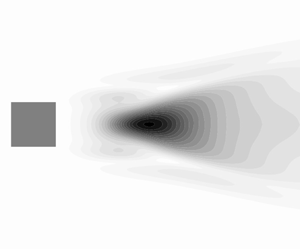
Figure 12 shows the values of the UTs in FANS at the fundamental frequency. These correspond to the highest-energy peak shown in figure 11. Significant axial velocity fluctuations are seen throughout the domain. Radial fluctuations are likewise present throughout but they become stronger in magnitude downstream due to the presence of vortex bubbles close to the wall. Finally, the azimuthal fluctuations start strongly near the inlet and diminish toward the wall. This gradual diminishing of fluctuations is due to the outward convection of the swirl noted by Herrada et al. (Reference Herrada, Del Pino and Ortega-Casanova2009).

Figure 12. Real value of FANS UTs of the swirling jet at the fundamental frequency in each coordinate direction: (a) axial, (b) radial and (c) azimuthal. Grey dashed line indicates  $U = 0$ which is the extent of VB bubble along the axis.
Figures 13(a) and 13(b) show the radial mean-flow convection and pressure gradient in the near-inlet region, respectively. These momentum fluxes are of considerably larger magnitude than the UT, peaking at over 45 times the maximum magnitude of the UT. The significant radial force fluctuations are due to the deflection of incoming flow against the VB bubble as indicated in figure 13. The interaction of the incoming jet with the VB bubble results in a large opposing pressure gradient. The relative magnitude of the forces combined with the phase of the UT (which can be compared through the sign of the value) shows that the pressure gradients dominate the convection in this region and drive the radial fluctuations. These radial fluctuations are important as they are related to the vortex bubbles that dominate the fluctuating flow. Thus, FANS can be used to elucidate the effect of large counteracting forces and compare them with the time-dependent term, which represents the fluctuations at that particular time scale.

Figure 13. Real value of FANS terms in the radial direction near the inlet of the swirling jet at the fundamental frequency: (a) mean-flow convection and (b) pressure gradient. Grey line shows the extent of VB bubble as in figure 12.
Herrada et al. (Reference Herrada, Del Pino and Ortega-Casanova2009) found that this jet flow is highly sensitive to changes in viscosity. The significant contribution of the viscous diffusion terms to the momentum transfer close to the inlet as seen in figure 14 implies a similar sensitivity. The phase and high magnitude of the azimuthal shear suggest that there is a dampening effect on the corresponding azimuthal fluctuations. This high shear stress shows the significant effect of the viscosity that results in high sensitivity of the flow physics to changes in the Reynolds number. In this way, FANS provides a platform to gain insight into the stability of the flow configuration.

Figure 14. Real value of FANS viscous diffusion term for the swirling jet in the azimuthal direction at the fundamental frequency.
The intermittent nature of the near-wall vortex bubbles observed in this flow results in a complicated time signature, where the vortex structures are observed across several frequencies. This suggests significant coupling between frequency components. To more thoroughly analyse this inter-frequency coupling of the jet flow and its relationship to the flow physics, Fourier stresses are analysed in more detail. Specifically, Fourier stresses represent the interactions that are generated by motion of the intermittent vortex bubbles.
The radial Fourier stress magnitudes for modes 2–4 are shown in figure 15. The radial terms are selected since they are characteristic of the vortex bubbles but not the swirling inlet flow. Notably, the vast majority of interactions occur outside of the recirculation region, located along the symmetry axis at  $y/h=0$. This follows with the radial convection of the velocity fluctuations as seen in figure 13, which is due to interaction of the jet with the recirculation region and the wall. The Fourier stresses have significant magnitude at each mode. This is consistent with the expectation of an energy cascade to higher frequencies resulting in a large number of modes. Regions of elevated Fourier stresses are localized well downstream of the inlet and outside of the recirculation region. This matches the expected location of enhanced interaction due to fluctuations induced by the vortex bubbles. Thus, FANS analysis of the convective coupling coincides with physical intuition about the interactions and time signature of the flow.

Figure 15. Fourier stress magnitude in the radial direction of the swirling jet for (a) mode 2, (b) mode 3 and (c) mode 4.
To further corroborate the influence of the vortex bubble on the inter-harmonic coupling, we explore the flow dynamics using BMD. Results of the bicorrelation coefficients  $\lambda _1$ for the bispectrum analysis of the jet are shown in figure 16. As this flow is periodic, the BMD mode bispectrum shows a cascade of harmonics, starting with triads involving the fundamental frequency $f^*=f\,h/U\approx 0.011$. This agrees with the observations of interactions between several modes as seen in figure 15.

Figure 16. Mode bispectrum of the swirling jet flow.
Figure 17 shows the BMD-calculated interaction maps for selected triads corresponding to  $(f^*_1=f^*, f^*_2 = f^*, f^*_3 = 2f^*)$, $(f^*_1=2f^*, f^*_2 = f^*, f^*_3 = 3f^*)$ and $(f^*_1=2f^*, f^*_2 = 2f^*, f^*_3 = 4f^*)$. Figure 17 presents the radial component of the interaction map for each triad. Similar to FANS, the interactions are found to remain outside of the recirculation region. This is due to the outward forcing of the flow as discussed above. This finding about the interactions supports the conclusions brought by Fourier stresses. The BMD-calculated interaction maps also show the localization of interactions downstream ( $x/h>5$) and outside of the recirculation region (figure 17). This suggests a relationship to the vortex bubbles similar to what was previously observed with radial Fourier stresses. The intermittent motion of the vortex bubbles results in significant interaction between modes, which then appears as enhanced triadic interactions or Fourier stresses detected by BMD and FANS, respectively.

Figure 17. Interaction maps in the radial direction of the swirling jet flow for triads (a)  $\psi _{1,1}$, (b) $\psi _{2,1}$ and (c) $\psi _{2,2}$.
3.3. Side-by-side cylinders
The final case considered is that of two side-by-side cylinders of diameter  $D$ at Reynolds number of $Re=U_\infty D/\nu = 90$. The cylinders are separated by a gap of $0.6D$. A representation of the computational domain is shown in figure 18. These settings and the corresponding mesh requirements were taken from Ma et al. (Reference Ma, Kang, Lim, Wu and Tutty2017), against which the results are verified. This flow configuration results in an asymmetric, irregularly oscillating wake characterized by multiple shedding processes and their interaction. There is vortex shedding behind each of the two cylinders, which then merges into a single Kármán-like street far downstream. There is also a ‘flip-flopping’ process where the wake asymmetry changes orientation (Ma et al. Reference Ma, Kang, Lim, Wu and Tutty2017). The flip-flop occurs randomly at a frequency much lower than that of the shedding (see Burattini & Agrawal Reference Burattini and Agrawal2013; Carini, Giannetti & Auteri Reference Carini, Giannetti and Auteri2014). As a result, there are multiple dominant frequencies. Depending on the location in the wake, the flow may be dominated by the low-frequency flip-flopping in between the cylinders, the high-frequency shedding process behind each of the cylinders or the moderate-frequency shedding process in the wake far from the cylinders due to wake merging. This case is selected to investigate the momentum transport processes detailed by FANS in a non-periodic case with multiple characteristic frequencies.

Figure 18. Two-dimensional simulation domain of side-by-side cylinders with a gap ratio of 0.6.
The spectrum of the flow energy fluctuations and the estimated power spectral density  $(S_{xx})$ of the drag and lift coefficients on the lower of the two cylinders are shown in figures 19(a) and 19(b), respectively. These broadband spectra show that the flow is irregular and not characterized by discrete frequency content. Within figure 19(a), there is a broadband spectrum centred about $f^*=0.07$, whereas the drag and lift spectrum shows dominant frequencies that are centred around 0.01 and 0.12. The lowest frequency $(f^*=fD/U_{\infty }\approx 0.01)$ corresponds to the flip-flopping process, which occurs on irregular intervals about this frequency. The moderate frequency shown in the energy spectrum corresponds to the moderate frequency shedding in the merged wake. The highest dominant frequencies in the lift and drag spectra ( $0.09 < f^* < 0.15$) correspond to vortex shedding on the cylinder body. The flip-flopping and two vortex production processes are analysed using the FANS framework. To simplify the analysis, representative frequencies are used for each process: $f^*=0.0105$ for flip-flopping, $f^*=0.075$ for vortex shedding from individual cylinders and $f^*=0.148$ for the Kármán-like street in the merged wake.

Figure 19. (a) Spectrum of flow energy fluctuations and (b) power spectral density of drag and lift coefficients on the lower cylinder.
Figure 20 shows the UT at  $f^*=0.0105$. This frequency corresponds to the flip-flopping process. Each of the lobes stemming from the gap represents a state of the flow, where the flow through the gap moves toward either the upper or lower cylinder at a given time. Ma et al. (Reference Ma, Kang, Lim, Wu and Tutty2017) discuss the importance of the gap flow in this regime. Figure 21 shows the momentum fluxes in the streamwise direction at the flip-flopping frequency, where the mean-flow convection (figure 21a), Fourier stresses (figure 21b) and pressure gradient (figure 21c) are significant. The diffusion does not contribute significantly to the transport process. These momentum fluxes show the importance of the gap flow to the flip-flopping effect. Large velocity gradients on the leeward side of the gap result in the large convective flux seen in figure 21(a) that sustains the switching process. These large velocity gradients are due to the combination of strong gap flow and tight spacing between the cylinders. This combination was highlighted by Ma et al. (Reference Ma, Kang, Lim, Wu and Tutty2017) as important to the instability that leads to the irregular flow, which is reflected here.

Figure 20. Real value of UT at flip-flopping frequency.

Figure 21. Real value of FANS terms in the streamwise direction corresponding to flip-flopping frequencies. (a) Mean-flow convection, (b) Fourier stresses and (c) pressure gradient.
There are also large-magnitude Fourier stresses at this frequency, immediately behind the cylinders. These stresses represent interactions of different frequencies within the bands of shedding and downstream vortex street frequencies. Since the bandwidth of the energy and force coefficient spectra is larger than the flip-flopping frequency, interactions between modes that lie within these bands result in Fourier stresses at the flip-flopping frequency.
Figure 22 shows the significant momentum fluxes at  $f^*=0.148$. This frequency corresponds to the cyclic shedding from the individual cylinders, which appears in the force spectra in figure 19(b). Evidence of shedding near the cylinders can be seen in the UT and pressure gradient in figure 22. This aligns with our expectations due to the force fluctuations at this frequency. This mode persists downstream (figure 22a). However, following Ma et al. (Reference Ma, Kang, Lim, Wu and Tutty2017), the two vortex streets from the individual cylinders interact in the wake. This interaction results in a Kármán-like vortex street at a frequency $f^*\approx 0.075$. Evidence of these interactions is discussed further below. The spatial-averaged spectrum of the wake velocity fluctuations thus shows a dominant energy concentration around $f^*\approx 0.075$ (figure 19a). However, since the forces arise mainly due to the flip-flopping instability and near-wake vortex shedding, the main contributions to the forces are around $f^*=0.011$ and $f^*=0.149$ (figure 19b).

Figure 22. Real values of streamwise momentum fluxes at  $f^*_m=0.148$: (a) UT, (b) mean-flow convection, (c) pressure and (d) Fourier stresses.
The Fourier stresses in figure 22(d) extend throughout the domain and have similar magnitude to the UT. The localization of wake phenomena, such as flip-flopping and the Kármán-like street, suggests that the Fourier stresses at this frequency are due to a broad range of interactions. The FANS technique provides a method to detect the primary mechanisms that contribute to these stresses in the form of individual terms in the Fourier stress term. Select terms are shown in figure 23. Modes are subscripted with their frequency due to the broadband spectrum of this flow. For instance,  $\hat {u}_{0.075}$ is the streamwise direction of the velocity Fourier mode at $f^*_m=0.075$. The Fourier stress term corresponding to the contribution of the downstream Kármán-like shedding frequency is represented in figure 23(a). The momentum flux due to this term shows increased magnitude in the region of $x/h>10$. The increased stress magnitude in this region is related to the interactions leading to the formation of the downstream merged vortices. Thus, it may be said that the primary driver of Fourier stresses in the far wake are due to contributions at $f^*=0.075$ due to the interactions leading to Kármán-like vortices downstream.

Figure 23. Real values of contributions to Fourier stresses at  $f^*=0.148$ in the streamwise direction, due to modes at indicated frequencies: (a) $(f^*_1=0.074, f^*_2=0.075)$ and (b) $(f^*_1=0.010, f^*_2=0.138)$.
Figure 23(b) shows the momentum flux in the same Fourier stress term due to the triad  $(f^*_1=0.010, f^*_2=0.138, f^*_3=0.148)$. The low frequency of $0.010$ corresponds to the flip-flopping process. This triad represents one of several similar interactions between these processes (other relevant triads are not shown here for brevity). Magnitude of the convective flux shown in figure 23(b) shows that the interaction between these modes is a significant source of momentum for the fluctuations at $f^*\approx 0.148$ immediately behind the cylinders. This suggests that the gap flow and flip-flopping process modulate the vortex shedding. This is supportive of the findings of Ma et al. (Reference Ma, Kang, Lim, Wu and Tutty2017), who also reported this modulation of the shedding behind the cylinders.
The energy transfer terms are also considered for this non-periodic case to assess the robustness of the FANS analysis. Figures 24(a) and 24(b) show the real and imaginary parts of the energy transfer terms, respectively. The symmetries expected from (2.13) are visible in the majority of the spectrum. However, this symmetry breaks down close to  $f_n = 0.075, f_k=-0.075$. This may be due to the integration domain. The components of this interaction have significant magnitude at the outlet in figures 22(a) and 23(a), which violates the assumption needed for the symmetry property in (2.13).

Figure 24. Real values of energy transfer terms  $\Delta E_n^k$ evaluated on the dual cylinder case. (a) Real part. (b) Imaginary part. Grey dashed line indicates where $f_n-f_k=0.075$. Interactions involving $f^*=0$ are omitted to highlight interactions between flow fluctuations.
Interactions involving  $f_n-f_k=0.075$ are particularly evident in the spectrum, as highlighted by the grey dashed line. Note that, by inherent symmetry, the energy transfer terms along the parallel line $f_k-f_n=0.075$ are interpreted similarly. The importance of the energy transfer along these lines is expected due to the large magnitude of the energy at this frequency, which corresponds to the shedding frequency, in figure 19(a). Similarly, the observed large magnitude of $E_n^k$ involving $f_k=0.075$ and $f_k=0.15$ is expected due to the vortex merging process in the wake. There are also concentrations of large-magnitude energy transfer terms involving low frequencies. This concentration is expected due to the interaction of the vortex shedding with the flip-flopping process.
The broadband spectrum of the fluctuations in the wake poses challenges for the interpretation of energy flow. This is because it spreads energy transfer information over several triads. However, in a particular neighbourhood, the sign of the energy transfer term remains consistent. For instance, the interactions in the neighbourhood of  $f_n=0.15, f_k=0.075$ have positive real value. This quality helps identify the direction of energy transfer, which can be deduced from the aggregation of multiple similar interactions. This allows for consistent conclusions about the energy transfer from these terms. Hence, the FANS energy transfer provides meaningful information in this irregularly cyclic case, suggesting that the technique is robust.
We once again utilize BMD to explore the flow dynamics. The spectrum of  $\lambda _1$ is shown in figure 25. There are local maxima in the bispectrum involving frequencies at $f^*\approx 0.073$. The diagonal and vertical bands of elevated correlation around these maxima may be due to spectral leakage (Schmidt Reference Schmidt2020). Locations of the maxima correspond to triads around $(f^*_1\approx 0.073, f^*_2 \approx 0.073, f^*_3 \approx 0.147)$ and $(f^*_1\approx 0.147, f^*_2 \approx -0.073, f^*_3 \approx 0.073)$. These triads involve the same frequencies, indicating that they are mirrored and capture the same interactions. The directions and magnitudes of the diagonal, horizontal and vertical bands of interactions captured by BMD are consistent with those from FANS in figure 24. For instance, BMD captures a diagonal band for $f_1+f_2=0.075$, which corresponds to the diagonal band seen for $f_n-f_k=0.075$ seen in FANS. The performance and conclusions of the two methods are similar for this case.

Figure 25. The BMD mode bispectrum for the dual cylinder case. The spectrum is blanked below  $10^{-5}$ to highlight strongly interacting triads.
Interaction maps corresponding to the triad  $(f^*_1\approx 0.073, f^*_2 \approx 0.073, f^*_3 \approx 0.147)$ are shown in figure 26. These correspond to the same wake processes discussed above using FANS. The exact listed frequency is slightly different from that of the FANS analysis due to the change in resolution, where BMD has lost some frequency resolution due to utilization of multiple windows. The interaction maps show significant triadic interaction beyond $x/D\approx 10$. This corresponds to the merger region, where the wakes of the individual cylinders combine and turn into a single Kármán-like street. The driving frequency of $f^*_1=0.073$ is characteristic of the vortex street. This frequency is outside of the range of important force spectra seen in figure 19. The resultant frequency of $f^*_3=0.147$ is characteristic of the cylinder shedding, which continues to have an influence downstream, as was deduced from the FANS analysis. The maps show interaction between these modes in the vortex street far from the cylinders. This interaction is consistent with the behaviour of the Fourier stresses in figure 23(a).

Figure 26. Bispectral interaction maps corresponding to far-wake frequencies, represented by the triad  $(f^*_1=0.073, f^*_2=0.073, f^*_3=0.147)$: (a) streamwise and (b) transverse components.
4. Conclusions
Periodic and turbulent flows exhibit complicated interactions that can be difficult to characterize. Here, the FANS equations are introduced to provide insight into the physics of flows with cyclic characteristics, including both regular (periodic) and irregular (non-periodic) recurrences. By combining information from Fourier modes and the Navier–Stokes equations, this method produces momentum equations for individual Fourier modes. The equations contain pressure, diffusion and convection terms that can be related to the velocity fluctuations and nonlinear interactions between modes. By treating the equations as a momentum budget, it is possible to directly compare different forces that contribute to fluctuations at a particular time scale. The FANS terms, and their analyses, can provide a more comprehensive interpretation of the flow, compared with other methods (e.g. BMD) that do not include spatial differentiation of the flow data as part of their analysis technique. The method directly addresses nonlinear interactions due to convection and relates them to the magnitude of other forces. The FANS formulation also includes phase information that can indicate when forces may be counteracting. This eases the physical interpretation of flow physics by isolating separate time scales and directly relating mode shapes to the governing equations. This is illustrated for periodic flows through case studies of the wake of a square cylinder and a swirling jet. The FANS analysis can also be utilized for irregularly oscillating flows, which is shown through the analysis of non-periodic flow around two side-by-side cylinders. The momentum equations of FANS can be used to find energy transfer terms between modes, which provide an opportunity to explore the direction in which energy flows between modes. Globally, these energy transfer terms can be separated into components that are directly related to the mode magnitude and dissipation, respectively. Momentum and energy analysis with FANS is shown to provide results consistent with those from other methods, such as BMD, in all three case studies considered here. However, it does so with fewer complexities and constraints than those associated with existing techniques. Particularly, FANS requires a single window of data, which significantly lowers the size of our dataset, and thus reduces the storage and processing requirements. Contrary to BMD, FANS does not entail irreversible and difficult-to-interpret processing steps. These constitute less intensive efforts in post-processing of the data by FANS analysis, which further benefits the physical interpretation by its direct correspondence to the terms in the governing equations for momentum conservation and energy balances. Yet, full implementation of this technique would require both pressure and velocity fields, which are easily obtained from simulations, but may require additional effort or treatment when considering experimental data. Using the FANS equations is a viable method to identify and describe the relationships between different processes in flows with regularly or irregularly repeating characteristics.
Funding
This work was funded by the Natural Sciences and Engineering Research Council of Canada.
Declaration of interests
The authors report no conflict of interest.
Appendix A. Derivation
The derivation begins by considering the incompressible Navier–Stokes equations of a Newtonian fluid:
 \begin{equation} \frac{\partial \boldsymbol{u}}{\partial t} + \boldsymbol{u}\boldsymbol{\cdot} \boldsymbol{\nabla} \boldsymbol{u} ={-}\boldsymbol{\nabla} p + \frac{1}{Re} \nabla^2 \boldsymbol{u}, \end{equation}
where  $\boldsymbol {u}$ is the instantaneous velocity vector field and $p$ is the pressure field. These quantities are non-dimensionalized with length scale $h$ and velocity scale $U_\infty$, so that the Reynolds number is $Re=U_\infty h / \nu$, where $\nu$ is the kinematic viscosity. The continuity equation has the form
 \begin{equation} \boldsymbol{\nabla} \boldsymbol{\cdot} \boldsymbol{u} = 0. \end{equation}
For the purposes of this method, the velocity and pressure fields are assumed to be representable as a Fourier series in time  $t$ with period $T$ and frequency increment $f = 1/T$:
 \begin{equation} \boldsymbol{u} = \sum_{m={-}\infty}^\infty \boldsymbol{\hat{u}}_m \exp(\,{\mathrm{j} 2{\rm \pi} m f t}) \end{equation}
and
 \begin{equation} p = \sum_{m={-}\infty}^\infty \hat{p}_m \exp(\,{\mathrm{j} 2{\rm \pi} m f t}). \end{equation}
The Fourier series coefficients,  $\boldsymbol {\hat {u}}_m$ and $\hat {p}_m$, are the velocity and pressure modes. These are complex-valued spatial functions. Here, $\mathrm {j}=\sqrt {-1}$ and $m$ is the mode number. Substituting the Fourier series representation of the flow fields into the Navier–Stokes equations:
 $$\begin{gather} \frac{\partial }{\partial t} \sum_{m={-}\infty}^\infty \boldsymbol{\hat{u}}_m \exp(\,{\mathrm{j} 2{\rm \pi} m f t})+ \sum_{m={-}\infty}^\infty \boldsymbol{\hat{u}}_m \exp(\,{\mathrm{j} 2{\rm \pi} m f t}) \boldsymbol{\cdot} \boldsymbol{\nabla} \sum_{m={-}\infty}^\infty \boldsymbol{\hat{u}}_m \exp(\,{\mathrm{j} 2{\rm \pi} m f t})\nonumber\\ ={-}\boldsymbol{\nabla} \sum_{m={-}\infty}^\infty \hat{p}_m \exp(\,{\mathrm{j} 2{\rm \pi} m f t}) + \frac{1}{Re} \nabla^2 \sum_{m={-}\infty}^\infty \boldsymbol{\hat{u}}_m \exp(\,{\mathrm{j} 2{\rm \pi} m f t}). \end{gather}$$
The basis functions of the Fourier space ( $\exp (\,\mathrm {j} 2{\rm \pi} m f t)$) are orthogonal under an integral inner product:
 \begin{equation} f\int_0^{T} \exp(\,{\mathrm{j} 2 {\rm \pi}f m t}) \exp({-\mathrm{j} 2 {\rm \pi}f\kern0.07em k t}) \,\text{d}t = \begin{cases} 1, & m=k \\ 0, & \text{otherwise} \end{cases}, \quad m, k \in \mathbb{Z}. \end{equation}
This allows us to isolate momentum equations for the individual modes ( $\boldsymbol {\hat {u}}_m$, $\hat {p}_m$). This is accomplished by multiplying both sides of (A5) with the basis function $f\exp ({-\mathrm {j} 2{\rm \pi} kf t})$ and integrating over the interval $[0, T]$:
 $$\begin{gather} f\int_T \exp({-\mathrm{j} 2{\rm \pi} k f t})\left( \underbrace{\frac{\partial }{\partial t} \sum_{m={-}\infty}^\infty \boldsymbol{\hat{u}}_m \exp(\,{\mathrm{j} 2{\rm \pi} m f t})}_{\text{unsteady term}} + \underbrace{\sum_{m={-}\infty}^\infty \boldsymbol{\hat{u}}_m \exp(\,{\mathrm{j} 2{\rm \pi} m f t}) \boldsymbol{\cdot} \boldsymbol{\nabla} \sum_{m={-}\infty}^\infty \boldsymbol{\hat{u}}_m \exp(\,{\mathrm{j} 2{\rm \pi} m f t})}_{\text{convection term}} \right) \,\text{d}t\nonumber\\ = f\int_T\exp({-\mathrm{j} 2{\rm \pi} k f t})\left( \underbrace{-\boldsymbol{\nabla} \sum_{m={-}\infty}^\infty \hat{p}_m \exp(\,{\mathrm{j} 2{\rm \pi} m f t})}_{\text{pressure term}} + \underbrace{\frac{1}{Re} \nabla^2 \sum_{m={-}\infty}^\infty \boldsymbol{\hat{u}}_m \exp(\,{\mathrm{j} 2{\rm \pi} m f t})}_{\text{diffusion term}} \right) \,\text{d}t. \end{gather}$$
The application of this integral is considered term by term.
A.1. Pressure and diffusion terms
The right-hand side of (A7) can be manipulated by commuting the integral and spatial derivative operators with the summations:
 \begin{align} &f\int_T\exp({-\mathrm{j} 2{\rm \pi} k f t})\left(-\boldsymbol{\nabla} \sum_{m={-}\infty}^\infty \hat{p}_m \exp(\,{\mathrm{j} 2{\rm \pi} m f t}) + \frac{1}{Re} \nabla^2 \sum_{m={-}\infty}^\infty \boldsymbol{\hat{u}}_m \exp(\,{\mathrm{j} 2{\rm \pi} m f t}) \right) \,\text{d}t \nonumber\\ &\quad={-}\sum_{m={-}\infty}^\infty f\int_T\exp({-\mathrm{j} 2{\rm \pi} k f t}) \exp(\,{\mathrm{j} 2{\rm \pi} m f t}) \boldsymbol{\nabla}\hat{p}_m \,\text{d}t\nonumber\\ &\qquad + \frac{1}{Re} \sum_{m={-}\infty}^\infty f\int_T \exp({-\mathrm{j} 2{\rm \pi} k f t}) \exp(\,{\mathrm{j} 2{\rm \pi} m f t}) \nabla^2 \boldsymbol{\hat{u}}_m \,\text{d}t \nonumber\\ &\quad={-}\sum_{m={-}\infty}^\infty \left(f\int_T\exp({-\mathrm{j} 2{\rm \pi} k f t}) \exp(\,{\mathrm{j} 2{\rm \pi} m f t}) \,\text{d}t\right) \left(\boldsymbol{\nabla}\hat{p}_m + \frac{1}{Re} \nabla^2 \boldsymbol{\hat{u}}_m \right). \end{align}
The integral in the final line is the inner product in (A6). As a result, the summation terms have a value of  $\boldsymbol {\nabla }\hat {p}_k + (1/Re) \nabla ^2 \boldsymbol {\hat {u}}_k$ when $k=m$ and vanish otherwise. With this fact, the right-hand side of (A7) becomes
 \begin{align} f\int_T &\exp({-\mathrm{j} 2{\rm \pi} k f t})\left(-\boldsymbol{\nabla} \sum_{m={-}\infty}^\infty \hat{p}_m \exp(\,{\mathrm{j} 2{\rm \pi} m f t}) + \frac{1}{Re} \nabla^2 \sum_{m={-}\infty}^\infty \boldsymbol{\hat{u}}_m \exp(\,{\mathrm{j} 2{\rm \pi} m f t}) \right) \,\text{d}t \nonumber\\ &\quad = \left(\boldsymbol{\nabla}\hat{p}_k + \frac{1}{Re} \nabla^2 \boldsymbol{\hat{u}}_k\right). \end{align}
A.2. Unsteady term
The unsteady term of (A7) can be written as
 \begin{align} &f\int_T\exp({-\mathrm{j} 2{\rm \pi} k f t}) \frac{\partial }{\partial t} \sum_{m={-}\infty}^\infty \boldsymbol{\hat{u}}_m \exp(\,{\mathrm{j} 2{\rm \pi} m f t}) \,\text{d}t \nonumber\\ &\quad = f\int_T\exp({-\mathrm{j} 2{\rm \pi} k f t}) \sum_{m={-}\infty}^\infty \boldsymbol{\hat{u}}_m \frac{\partial }{\partial t}\left( \exp(\,{\mathrm{j} 2{\rm \pi} m f t}) \right) + \frac{\partial }{\partial t}\left(\boldsymbol{\hat{u}}_m\right) \exp(\,{\mathrm{j} 2{\rm \pi} m f t}) \,\text{d}t. \end{align}
The  $({\partial }/{\partial t})(\boldsymbol {\hat {u}}_m)$ term vanishes since the Fourier modes are functions of space only. Thus, the inner product can be written as
 \begin{equation} = f\int_T\exp({-\mathrm{j} 2{\rm \pi} k f t}) \sum_{m={-}\infty}^\infty \boldsymbol{\hat{u}}_m \left(\,\mathrm{j} 2{\rm \pi} m f \right) \exp(\,{\mathrm{j} 2{\rm \pi} m f t}) \,\text{d}t. \end{equation}
This once again isolates  $\boldsymbol {\hat {u}}_k$ due to the inner product property (A6). As a result,
 \begin{equation} f\int_T\exp({-\mathrm{j} 2{\rm \pi} k f t}) \frac{\partial }{\partial t} \sum_{m={-}\infty}^\infty \boldsymbol{\hat{u}}_m \exp(\,{\mathrm{j} 2{\rm \pi} m f t}) \,\text{d}t = \mathrm{j} 2{\rm \pi} k f \boldsymbol{\hat{u}}_k. \end{equation}
A.3. Convection term
The nonlinearity of the convection term makes its treatment more complicated. With the inner product from (A7), the convection term is
 \begin{gather} f\int_T \exp({-\mathrm{j} 2{\rm \pi} k f t}) \sum_{m={-}\infty}^\infty \boldsymbol{\hat{u}}_m \exp(\,{\mathrm{j} 2{\rm \pi} m f t}) \boldsymbol{\cdot} \boldsymbol{\nabla} \sum_{n={-}\infty}^\infty \boldsymbol{\hat{u}}_n \exp(\,{\mathrm{j} 2{\rm \pi} n f t}) \,\text{d}t \end{gather}
 \begin{gather} = f\int_T \sum_{m={-}\infty}^\infty\sum_{n={-}\infty}^\infty \exp({-\mathrm{j} 2{\rm \pi} k f t}) \exp(\,{\mathrm{j} 2{\rm \pi} n f t}) \exp(\,{\mathrm{j} 2{\rm \pi} m f t}) \left(\boldsymbol{\hat{u}}_m \boldsymbol{\cdot} \boldsymbol{\nabla} \boldsymbol{\hat{u}}_n \right) \,\text{d}t \end{gather}
 \begin{gather} = \sum_{m={-}\infty}^\infty\sum_{n={-}\infty}^\infty f\int_T \exp(\,{\mathrm{j} 2{\rm \pi} ({-}k+n+m) f t}) \,\text{d}t \left(\boldsymbol{\hat{u}}_m \boldsymbol{\cdot} \boldsymbol{\nabla} \boldsymbol{\hat{u}}_n \right). \end{gather}
Per (A6), the integral is non-zero only when  $m=k-n$. This reduces the double summation $\sum _m\sum _n$ to a single summation $\sum _{n}$:
 \begin{align} f\int_T \exp({-\mathrm{j} 2{\rm \pi} k f t}) \sum_{m={-}\infty}^\infty \boldsymbol{\hat{u}}_m \exp(\,{\mathrm{j} 2{\rm \pi} m f t}) \boldsymbol{\cdot} \boldsymbol{\nabla} \sum_{n={-}\infty}^\infty \boldsymbol{\hat{u}}_n \exp(\,{\mathrm{j} 2{\rm \pi} n f t}) \,\text{d}t \!=\! \sum_{n={-}\infty}^\infty \boldsymbol{\hat{u}}_{k-n} \boldsymbol{\cdot} \boldsymbol{\nabla} \boldsymbol{\hat{u}}_m. \end{align}
 Isolating the terms involving mode  $k$ and the mean flow in this summation highlights the effect of inter-frequency coupling on the momentum transfer:
 \begin{equation} \sum_{n={-}\infty}^\infty \boldsymbol{\hat{u}}_{k-n} \boldsymbol{\cdot} \boldsymbol{\nabla} \boldsymbol{\hat{u}}_n = \boldsymbol{\hat{u}}_{k} \boldsymbol{\cdot} \boldsymbol{\nabla} \boldsymbol{U} + \boldsymbol{U} \boldsymbol{\cdot} \boldsymbol{\nabla} \boldsymbol{\hat{u}}_k + \sum_{\substack{n={-}\infty \\ n \neq 0,k}}^\infty \boldsymbol{\hat{u}}_{k-n} \boldsymbol{\cdot} \boldsymbol{\nabla} \boldsymbol{\hat{u}}_n, \end{equation}
where  $\boldsymbol {U}$ is the mean velocity. The final term on the right-hand side represents the effect on mode $k$ of coupling between other modes. These interactions are referred to as the Fourier stresses as an analogy to the Reynolds stresses. This term can be written as
 \begin{equation} \tilde{\chi}[\boldsymbol{\hat{u}}_k] = \sum_{\substack{n={-}\infty \\ n \neq 0,k}}^\infty \boldsymbol{\hat{u}}_{k-n} \boldsymbol{\cdot} \boldsymbol{\nabla} \boldsymbol{\hat{u}}_n. \end{equation}
 Using the results of (A9), (A12), (A17) and (A18), the momentum equation corresponding to mode  $\boldsymbol {\hat {u}}_k$ is
 \begin{equation} \mathrm{j} 2{\rm \pi} k f \boldsymbol{\hat{u}}_k + \boldsymbol{\hat{u}}_{k} \boldsymbol{\cdot} \boldsymbol{\nabla} \boldsymbol{U} + \boldsymbol{U} \boldsymbol{\cdot} \boldsymbol{\nabla} \boldsymbol{\hat{u}}_k + \tilde{\chi}[\boldsymbol{\hat{u}}_k] ={-}\boldsymbol{\nabla} \hat{p}_k + \frac{1}{Re}\nabla^2 \boldsymbol{\hat{u}}_k. \end{equation}
A.4. Continuity
Each velocity mode is divergence-free. Using the Fourier series representation in the continuity equation, it becomes
 \begin{equation} \boldsymbol{\nabla} \boldsymbol{\cdot} \boldsymbol{u} = \boldsymbol{\nabla} \boldsymbol{\cdot} \sum_{m={-}\infty}^\infty \boldsymbol{\hat{u}}_m \exp(\,{\mathrm{j} 2{\rm \pi} m f t}) = 0. \end{equation}
To isolate an equation for mode  $\boldsymbol {\hat {u}}_k$, an inner product of this equation is applied with the basis function $\exp ({-\mathrm {j} 2{\rm \pi} k ft})$. This yields
 \begin{align} &\int_T
\exp({-\mathrm{j} 2{\rm \pi} k ft}) \boldsymbol{\nabla}
\boldsymbol{\cdot} \sum_{m={-}\infty}^\infty
\boldsymbol{\hat{u}}_m \exp(\,{\mathrm{j} 2{\rm \pi} m f t})
\,\text{d}t\nonumber\\ &\quad = \int_T \boldsymbol{\nabla} \boldsymbol{\cdot}
\sum_{m={-}\infty}^\infty \left(\boldsymbol{\hat{u}}_m
\exp(\,{\mathrm{j} 2{\rm \pi} m f t}) \exp({-\mathrm{j} 2{\rm \pi} k
ft})\right) \,\text{d}t\nonumber\\ &\quad = \boldsymbol{\nabla}
\boldsymbol{\cdot} \sum_{m={-}\infty}^\infty \int_T
\boldsymbol{\hat{u}}_m \exp(\,{\mathrm{j} 2{\rm \pi} (m-k) f t})
\,\text{d}t = \boldsymbol{\nabla} \boldsymbol{\cdot}
\sum_{m={-}\infty}^\infty \int_T \exp(\,{\mathrm{j} 2{\rm \pi}
(m-k) f t}) \,\text{d}t \boldsymbol{\hat{u}}_m.
\end{align}
\begin{align} &\int_T
\exp({-\mathrm{j} 2{\rm \pi} k ft}) \boldsymbol{\nabla}
\boldsymbol{\cdot} \sum_{m={-}\infty}^\infty
\boldsymbol{\hat{u}}_m \exp(\,{\mathrm{j} 2{\rm \pi} m f t})
\,\text{d}t\nonumber\\ &\quad = \int_T \boldsymbol{\nabla} \boldsymbol{\cdot}
\sum_{m={-}\infty}^\infty \left(\boldsymbol{\hat{u}}_m
\exp(\,{\mathrm{j} 2{\rm \pi} m f t}) \exp({-\mathrm{j} 2{\rm \pi} k
ft})\right) \,\text{d}t\nonumber\\ &\quad = \boldsymbol{\nabla}
\boldsymbol{\cdot} \sum_{m={-}\infty}^\infty \int_T
\boldsymbol{\hat{u}}_m \exp(\,{\mathrm{j} 2{\rm \pi} (m-k) f t})
\,\text{d}t = \boldsymbol{\nabla} \boldsymbol{\cdot}
\sum_{m={-}\infty}^\infty \int_T \exp(\,{\mathrm{j} 2{\rm \pi}
(m-k) f t}) \,\text{d}t \boldsymbol{\hat{u}}_m.
\end{align}
Once again the integral vanishes except for  $k=m$:
 \begin{equation} \int_T \exp({-\mathrm{j} 2{\rm \pi} k ft}) \boldsymbol{\nabla} \boldsymbol{\cdot} \sum_{m={-}\infty}^\infty \boldsymbol{\hat{u}}_m \exp(\,{\mathrm{j} 2{\rm \pi} m f t}) \,\text{d}t = \boldsymbol{\nabla} \boldsymbol{\cdot} \boldsymbol{\hat{u}}_k. \end{equation}
Likewise, the integral of the right-hand side of the continuity equation is zero:
 \begin{equation} \int_T \exp({-\mathrm{j} 2{\rm \pi} k ft}) (0) \,\text{d} t = 0. \end{equation}
Equating the left- and right-hand sides, we have
 \begin{equation} \boldsymbol{\nabla} \boldsymbol{\cdot} \boldsymbol{\hat{u}}_k = 0. \end{equation}
This can be interpreted as a set of continuity equations that the velocity modes each satisfy independently.
Appendix B. Energy transfer derivation
In order to construct the turbulent kinetic energy from the modes, the inner product of  $\boldsymbol {\hat {u}}_k^*$ with the FANS equation for mode $k$ is taken:
 \begin{align} &\mathrm{j} 2{\rm \pi} f\kern0.07em k\boldsymbol{\hat{u}}_k^* \boldsymbol{\cdot} \boldsymbol{\hat{u}}_k + \boldsymbol{\hat{u}}_k^* \boldsymbol{\cdot} \left(\left(\boldsymbol{U}\boldsymbol{\cdot} \boldsymbol{\nabla}\right) \boldsymbol{\hat{u}}_k + \left(\boldsymbol{\hat{u}}_k \boldsymbol{\cdot} \boldsymbol{\nabla}\right) \boldsymbol{U}\right)\nonumber\\ &\quad ={-}\boldsymbol{\hat{u}}_k^* \boldsymbol{\cdot} \boldsymbol{\nabla} \hat{p}_k + \nu \boldsymbol{\hat{u}}_k^* \boldsymbol{\cdot} \nabla^2 \boldsymbol{\hat{u}}_k - \boldsymbol{\hat{u}}_k^*\boldsymbol{\cdot} \sum_{\substack{n={-}\infty \\ n \neq 0,k}}^\infty \left(\boldsymbol{\hat{u}}_{k-n}\boldsymbol{\cdot} \boldsymbol{\nabla}\right) \boldsymbol{\hat{u}}_n. \end{align}
Here, the inner product between a vector  $\boldsymbol {a}$ and a vector $\boldsymbol {b}$ is $\boldsymbol {a}\boldsymbol {\cdot } \boldsymbol {b}=a_ib_i$ even for complex-valued vectors. For the purposes of the following derivation, there is no mathematical difference between the mean-flow and modal convection terms (second and third terms of the left-hand side and the last term on the right-hand side), so they will be recombined:
 \begin{equation} \mathrm{j} 2{\rm \pi} f\kern0.07em k\boldsymbol{\hat{u}}_k^* \boldsymbol{\cdot} \boldsymbol{\hat{u}}_k + \boldsymbol{\hat{u}}_k^*\boldsymbol{\cdot} \sum_{n={-}\infty }^\infty \left(\boldsymbol{\hat{u}}_{k-n}\boldsymbol{\cdot} \boldsymbol{\nabla} \right) \boldsymbol{\hat{u}}_n ={-}\boldsymbol{\hat{u}}_k^* \boldsymbol{\cdot} \boldsymbol{\nabla} \hat{p}_k + \nu \boldsymbol{\hat{u}}_k^* \boldsymbol{\cdot} \nabla^2 \boldsymbol{\hat{u}}_k. \end{equation}
However, it should still be noted that the interpretation of the mean-flow terms will still differ. Most of the terms in this equation are extremely straightforward to manipulate into simpler forms and so will not be considered here. In terms of looking at exchange between modes, only the convection term  $\boldsymbol {\hat {u}}_k^*\boldsymbol {\cdot } \sum _{n=-\infty }^\infty \boldsymbol {\hat {u}}_{k-n}\boldsymbol {\cdot } \boldsymbol {\nabla } \boldsymbol {\hat {u}}_n$ is relevant. A single term of this summation defines the local energy transfer between modes $n$ and $k$,
$k$,  $\Delta e_n^k$:
 \begin{equation} \Delta e_n^k = \boldsymbol{\hat{u}}_k^*\boldsymbol{\cdot} \left( \left(\boldsymbol{\hat{u}}_{k-n}\boldsymbol{\cdot} \boldsymbol{\nabla}\right) \boldsymbol{\hat{u}}_n\right). \end{equation}
There appears to be a symmetry between this term and one that appears in the equation for  $\boldsymbol {\hat {u}}_{-n}$:
 \begin{align} {-}\mathrm{j} 2{\rm \pi} f n\boldsymbol{\hat{u}}_{{-}n}^* \boldsymbol{\cdot} \boldsymbol{\hat{u}}_{{-}n} + \boldsymbol{\hat{u}}_{{-}n}^*\boldsymbol{\cdot} \sum_{k={-}\infty }^\infty \left(\boldsymbol{\hat{u}}_{k-n}\boldsymbol{\cdot} \boldsymbol{\nabla} \right) \boldsymbol{\hat{u}}_{{-}k}={-}\boldsymbol{\hat{u}}_{{-}n}^* \boldsymbol{\cdot} \boldsymbol{\nabla} \hat{p}_{{-}n} + \nu \boldsymbol{\hat{u}}_{{-}n}^* \boldsymbol{\cdot} \nabla^2 \boldsymbol{\hat{u}}_{{-}n}. \end{align}
The summation index of the final term was intentionally chosen as  $k$ for easy comparison between the equations. Once again isolating a single term from the Fourier stresses:
 \begin{equation} \Delta e^{{-}n}_{{-}k} = \boldsymbol{\hat{u}}_{{-}n}^*\boldsymbol{\cdot} \left( \left(\boldsymbol{\hat{u}}_{k-n}\boldsymbol{\cdot} \boldsymbol{\nabla}\right) \boldsymbol{\hat{u}}_{{-}k}\right). \end{equation}
Applying the chain rule:
 \begin{equation} \boldsymbol{\hat{u}}_{{-}n}^*\boldsymbol{\cdot} \left( \left(\boldsymbol{\hat{u}}_{k-n}\boldsymbol{\cdot} \boldsymbol{\nabla}\right) \boldsymbol{\hat{u}}_{{-}k}\right) = \boldsymbol{\nabla} \boldsymbol{\cdot} \left( \boldsymbol{\hat{u}}_{k-n} \left( \boldsymbol{\hat{u}}_{{-}n}^* \boldsymbol{\cdot} \boldsymbol{\hat{u}}_{{-}k}\right)\right) - \boldsymbol{\hat{u}}_{{-}k} \boldsymbol{\cdot} \left(\boldsymbol{\hat{u}}_{k-n}\boldsymbol{\cdot} \boldsymbol{\nabla} \right) \boldsymbol{\hat{u}}_{{-}n}^*. \end{equation}
For real signals,  $\boldsymbol {\hat {u}}_{-k}=\boldsymbol {\hat {u}}^*_k$ and $\boldsymbol {\hat {u}}_{-n}^*=\boldsymbol {\hat {u}}_n$. Therefore $\boldsymbol {\hat {u}}_{-k} \boldsymbol {\cdot } (\boldsymbol {\hat {u}}_{k-n}\boldsymbol {\cdot } \boldsymbol {\nabla } ) \boldsymbol {\hat {u}}_{-n}^*=\boldsymbol {\hat {u}}_{k}^* \boldsymbol {\cdot } (\boldsymbol {\hat {u}}_{k-n}\boldsymbol {\cdot } \boldsymbol {\nabla } ) \boldsymbol {\hat {u}}_{n}$ $=\Delta e_n^k$. As a result, $\Delta e^{-n}_{-k}$ is
 \begin{equation} \Delta e^{{-}n}_{{-}k} = \boldsymbol{\nabla} \boldsymbol{\cdot} \left( \boldsymbol{\hat{u}}_{k-n} \left( \boldsymbol{\hat{u}}_{{-}n}^* \boldsymbol{\cdot} \boldsymbol{\hat{u}}_{{-}k}\right)\right) - \Delta e_n^k. \end{equation}
Since  $\Delta e_n^k$ appears in the equations for both $\boldsymbol {\hat {u}}_{-n}$ and $\boldsymbol {\hat {u}}_k$ with opposite sign, it can be considered to be the energy transfer term. This naming is used as the term ‘transfers’ energy between modal equations. This is analogous to the role of the production term of the turbulent kinetic energy equations (Durbin & Pettersson Reference Durbin and Pettersson2011).
The primary concern here is the characteristics of the global energy transfer between  $k$ and $n$. The energy transfer between mode $\boldsymbol {\hat {u}}_k$ and mode $\boldsymbol {\hat {u}}_n$ from the equation for mode $k$ is defined as
 \begin{equation} \Delta E^k_n = \int_\varOmega \boldsymbol{\hat{u}}_k^*\boldsymbol{\cdot} \left( \left(\boldsymbol{\hat{u}}_{k-n}\boldsymbol{\cdot} \boldsymbol{\nabla}\right) \boldsymbol{\hat{u}}_n\right) \,\text{d}V. \end{equation}
 Similarly, again given real input signals, the transfer between the same two modes from the equation for mode  $-n$ is
 \begin{align} \Delta E_{{-}k}^{{-}n}
&= \int_\varOmega \boldsymbol{\hat{u}}_{n}\boldsymbol{\cdot}
\left( \left(\boldsymbol{\hat{u}}_{k-n}\boldsymbol{\cdot}
\boldsymbol{\nabla}\right)
\boldsymbol{\hat{u}}_{k}^*\right) \,\text{d}V =
\left(\Delta E_{k}^{n}\right)^*\nonumber\\ &= \int_\varOmega
\boldsymbol{\nabla} \boldsymbol{\cdot} \left(
\boldsymbol{\hat{u}}_{k-n} \left( \boldsymbol{\hat{u}}_{n}
\boldsymbol{\cdot} \boldsymbol{\hat{u}}_k^*\right)\right) -
\boldsymbol{\hat{u}}_k^* \boldsymbol{\cdot}
\left(\boldsymbol{\hat{u}}_{k-n}\boldsymbol{\cdot}
\boldsymbol{\nabla} \right) \boldsymbol{\hat{u}}_{n}
\,\text{d}V\nonumber\\ &= \int_{\partial\varOmega}
\left(\boldsymbol{\hat{u}}_{n} \boldsymbol{\cdot}
\boldsymbol{\hat{u}}_k^*\right)
\left(\boldsymbol{\hat{u}}_{k-n} \boldsymbol{\cdot}
\boldsymbol{n}\right) \,\text{d}S - \Delta E^k_n.
\end{align}
\begin{align} \Delta E_{{-}k}^{{-}n}
&= \int_\varOmega \boldsymbol{\hat{u}}_{n}\boldsymbol{\cdot}
\left( \left(\boldsymbol{\hat{u}}_{k-n}\boldsymbol{\cdot}
\boldsymbol{\nabla}\right)
\boldsymbol{\hat{u}}_{k}^*\right) \,\text{d}V =
\left(\Delta E_{k}^{n}\right)^*\nonumber\\ &= \int_\varOmega
\boldsymbol{\nabla} \boldsymbol{\cdot} \left(
\boldsymbol{\hat{u}}_{k-n} \left( \boldsymbol{\hat{u}}_{n}
\boldsymbol{\cdot} \boldsymbol{\hat{u}}_k^*\right)\right) -
\boldsymbol{\hat{u}}_k^* \boldsymbol{\cdot}
\left(\boldsymbol{\hat{u}}_{k-n}\boldsymbol{\cdot}
\boldsymbol{\nabla} \right) \boldsymbol{\hat{u}}_{n}
\,\text{d}V\nonumber\\ &= \int_{\partial\varOmega}
\left(\boldsymbol{\hat{u}}_{n} \boldsymbol{\cdot}
\boldsymbol{\hat{u}}_k^*\right)
\left(\boldsymbol{\hat{u}}_{k-n} \boldsymbol{\cdot}
\boldsymbol{n}\right) \,\text{d}S - \Delta E^k_n.
\end{align}
Many cases will have approximately steady or no-slip boundaries almost everywhere, meaning  $\boldsymbol {\hat {u}}_k=0$ for $k\neq 0$. Therefore the surface integral will go to zero with a sufficiently large integration domain. This indicates that globally, $\Delta E^k_n$ appears in (B2) for $k$ and $-\Delta E^k_n$ appears in (B4) for $-n$. This indicates that the direction of energy transfer can be detected from the value of $\Delta E_n^k$. This requires consideration of its phase and the values of $n$ and $k$. The above derivation assumes the time decomposition of a real velocity field; however, it may be shown that these properties also hold for a spatially decomposed, and therefore complex, velocity field. For an illustration of this process, we start with decomposing the velocity field into a Fourier series in time and space:
 \begin{equation} \boldsymbol{u}(\boldsymbol{x, t}) = \sum_{\boldsymbol{\zeta} \in \mathcal{Z}^3}\sum_{k ={-}\infty}^\infty \boldsymbol{\hat{u}}_{k,\boldsymbol{\zeta}} \exp\left({\left(\,{\mathrm{j}2{\rm \pi} \left(f_k t + \boldsymbol{\lambda}_{\boldsymbol{\zeta}} \boldsymbol{\cdot} \boldsymbol{x} \right)}\right)}\right), \end{equation}
where  $f_k = k/T$ is a frequency and $\boldsymbol {\lambda }_{\boldsymbol {\zeta }} = [\zeta _x / L_x, \zeta _y/L_y, \zeta _z/L_z ]^{\rm T}$ is a vector of wavelengths, $T$ is the period, $\boldsymbol {\zeta }$ is a vector of integer wavenumbers and $L_x, L_y$ and $L_z$ are wavelengths in the $x$,
$x$,  $y$ and $z$ directions, respectively. The energy transfer term that results from the spatial and temporal decomposition of the Navier–Stokes equations is
 \begin{equation} \Delta E_{n,\boldsymbol{\eta}}^{k,\boldsymbol{\zeta}} = \mathrm{j}2{\rm \pi} \boldsymbol{\hat{u}}^*_{k,\boldsymbol{\zeta}}\boldsymbol{\cdot}\left(\left(\boldsymbol{\hat{u}}_{k-n,\boldsymbol{\zeta}-\boldsymbol{\eta}} \boldsymbol{\cdot} \boldsymbol{\lambda}_{\boldsymbol{\zeta}}\right)\boldsymbol{\hat{u}}_{n,\boldsymbol{\eta}}\right) = \mathrm{j}2{\rm \pi} \left(\boldsymbol{\hat{u}}_{k,\boldsymbol{\zeta}}^*\boldsymbol{\cdot} \boldsymbol{\hat{u}}_{n,\eta}\right)\left(\boldsymbol{\hat{u}}_{k-n,\boldsymbol{\zeta}-\boldsymbol{\eta}}\boldsymbol{\cdot} \boldsymbol{\lambda}_{\boldsymbol{\eta}}\right). \end{equation}
To check the symmetry property in this case, we explore  $\Delta E^{-n,-\boldsymbol {\eta }}_{-k,-\boldsymbol {\zeta }}$:
 \begin{equation} \Delta E^{{-}n,-\boldsymbol{\eta}}_{{-}k,-\boldsymbol{\zeta}} = \mathrm{j}2{\rm \pi} \left(\boldsymbol{\hat{u}}_{{-}k,-\boldsymbol{\zeta}}\boldsymbol{\cdot} \boldsymbol{\hat{u}}_{{-}n,-\eta}^*\right)\left(\boldsymbol{\hat{u}}_{{-}n+k,-\boldsymbol{\eta}+\boldsymbol{\zeta}}\boldsymbol{\cdot} \boldsymbol{\lambda}_{-\boldsymbol{\zeta}}\right). \end{equation}
There are a few properties to note:
 \begin{equation} \boldsymbol{\hat{u}}_{{-}k,-\boldsymbol{\zeta}}^* = \boldsymbol{\hat{u}}_{k,\boldsymbol{\zeta}}, \quad \boldsymbol{\lambda}_{-\boldsymbol{\zeta}} ={-}\boldsymbol{\lambda}_{\boldsymbol{\zeta}},\quad \boldsymbol{\lambda}_{\boldsymbol{\eta} + \boldsymbol{\zeta}} = \boldsymbol{\lambda}_{\boldsymbol{\eta}} + \boldsymbol{\lambda}_{\boldsymbol{\zeta}},\quad \boldsymbol{\lambda}_{\boldsymbol{\zeta}} \boldsymbol{\cdot} \boldsymbol{\hat{u}}_{k,\boldsymbol{\zeta}} = 0. \end{equation}
Keeping these in mind, we return to (B12) and can show that
 \begin{equation} \Delta E^{{-}n,-\boldsymbol{\eta}}_{{-}k,-\boldsymbol{\zeta}} ={-}\mathrm{j}2{\rm \pi} \left(\boldsymbol{\hat{u}}_{k,\boldsymbol{\zeta}}^*\boldsymbol{\cdot} \boldsymbol{\hat{u}}_{n,\eta}\right)\left(\boldsymbol{\hat{u}}_{k-n,\boldsymbol{\zeta}-\boldsymbol{\eta}}\boldsymbol{\cdot}\boldsymbol{\lambda}_{\boldsymbol{\eta}}\right) ={-}\Delta E_{n,\boldsymbol{\eta}}^{k,\boldsymbol{\zeta}}. \end{equation}
Therefore  $\Delta E_{n,\boldsymbol {\eta }}^{k,\boldsymbol {\zeta }} = -\Delta E^{-n,-\boldsymbol {\eta }}_{-k,-\boldsymbol {\zeta }} = -(\Delta E^{n,\boldsymbol {\eta }}_{k,\boldsymbol {\zeta }})^*$, which is a similar symmetry property to that found in the previous revision for non-spatially decomposed data. Consequently, the symmetry may be generalized to multiple-dimensional Fourier decompositions. This provides a method for discussing energy transfer over both multiple length and time scales.
Appendix C. Energy transfer properties
For a global picture of the energy transfer, the volume integral of (B2) is taken. Taking the volume integral for a global picture:
 \begin{align} \int_\varOmega \mathrm{j} 2{\rm \pi} f\kern0.07em k\boldsymbol{\hat{u}}_k^* \boldsymbol{\cdot} \boldsymbol{\hat{u}}_k + \boldsymbol{\hat{u}}_k^*\boldsymbol{\cdot} \sum_{n={-}\infty}^\infty \left(\boldsymbol{\hat{u}}_{k-n}\boldsymbol{\cdot} \boldsymbol{\nabla}\right) \boldsymbol{\hat{u}}_n \,\text{d}V = \int_\varOmega -\boldsymbol{\hat{u}}_k^* \boldsymbol{\cdot} \boldsymbol{\nabla} \hat{p}_k + \nu \boldsymbol{\hat{u}}_k^* \boldsymbol{\cdot} \nabla^2 \boldsymbol{\hat{u}}_k \,\text{d}V. \end{align}
We briefly look at some of the terms separately in order to make some simplifications. Starting with the pressure term:
 \begin{equation} \int_\varOmega \boldsymbol{\hat{u}}_k^* \boldsymbol{\cdot}\left( \boldsymbol{\nabla} \hat{p}_k\right) \,\text{d}V = \int_\varOmega \boldsymbol{\nabla} \boldsymbol{\cdot} \left( \boldsymbol{\hat{u}}_k^* \hat{p}_k\right) - \hat{p}_k\boldsymbol{\nabla} \boldsymbol{\cdot} \boldsymbol{\hat{u}}_k^* \,\text{d}V. \end{equation}
The second term on the right-hand side is zero since the modes are incompressible. For the first term, we consider the Gauss theorem:
 \begin{equation} = \int_{\partial \varOmega} \hat{p}_k \boldsymbol{\hat{u}}_k^* \boldsymbol{\cdot} \boldsymbol{n} \,\text{d}S. \end{equation}
Since this term only acts at the boundaries, it may be understood as a transport term. Additionally, we typically consider steady boundary conditions, so this integral vanishes when  $k\neq 0$. As a result,
 \begin{equation} \int_\varOmega \boldsymbol{\hat{u}}_k^* \boldsymbol{\cdot} \left(\boldsymbol{\nabla} \hat{p}_k\right) \,\text{d}V = 0. \end{equation}
Continuing with the diffusion term, we use the product rule:
 $$\begin{gather} \int_\varOmega \nu \boldsymbol{\hat{u}}_k^* \boldsymbol{\cdot} \left(\nabla^2 \boldsymbol{\hat{u}}_k \right)\,\text{d}V = \int_\varOmega \nu\boldsymbol{\nabla} \boldsymbol{\cdot} \left( \left(\boldsymbol{\nabla} \boldsymbol{\hat{u}}_k\right) \boldsymbol{\hat{u}}_k^* \right) - \nu (\boldsymbol{\nabla} \boldsymbol{\hat{u}}_k^*):(\boldsymbol{\nabla}\boldsymbol{\hat{u}}_k) \,\text{d}V\nonumber\\ = \int_{\partial\varOmega} \nu\left( \left(\boldsymbol{\nabla} \boldsymbol{\hat{u}}_k\right) \boldsymbol{\hat{u}}_k^* \right)\boldsymbol{\cdot} \boldsymbol{n} \,\text{d}S - \nu \int_\varOmega (\boldsymbol{\nabla} \boldsymbol{\hat{u}}_k^*):(\boldsymbol{\nabla}\boldsymbol{\hat{u}}_k) \,\text{d}V. \end{gather}$$
The first term is a transport term which vanishes when  $k\neq 0$. Since $\boldsymbol {\hat {u}}_k^*=\boldsymbol {\hat {u}}_{-k}$, and the second term is the Frobenius norm of $\boldsymbol {\nabla } \boldsymbol {\hat {u}}_k$, defined as
 \begin{equation} \lVert \boldsymbol{\nabla} \boldsymbol{\hat{u}}_k \rVert^2_F = (\boldsymbol{\nabla} \boldsymbol{\hat{u}}_{k})^*:(\boldsymbol{\nabla}\boldsymbol{\hat{u}}_k). \end{equation}
As a result, the diffusion term evaluates to
 \begin{equation} \int_\varOmega \nu \boldsymbol{\hat{u}}_k^* \boldsymbol{\cdot} \left(\nabla^2 \boldsymbol{\hat{u}}_k\right) \,\text{d}V ={-}\nu \int_\varOmega \lVert \boldsymbol{\nabla} \boldsymbol{\hat{u}}_k \rVert^2_F \,\text{d} V. \end{equation}
This means that the diffusion term is purely real, since the Frobenius norm is strictly real and positive.
Applying the results (C4) and (C7), alongside the definition of  $\Delta E_n^k$, to (C1):
 \begin{equation} \int_\varOmega \mathrm{j} 2{\rm \pi} f\kern0.07em k \lVert \boldsymbol{\hat{u}}_k \rVert^2 \,\text{d}V + \sum_{n={-}\infty}^\infty \Delta E_n^k ={-}\nu \int_\varOmega \lVert \boldsymbol{\nabla} \boldsymbol{\hat{u}}_k \rVert^2_F \,\text{d} V. \end{equation}
Clearly, the first term, from the unsteady part of the equation, is strictly imaginary. The third term, from diffusion, is strictly real. The second term, representing energy transfers due to convective coupling between modes, has both real and imaginary parts. In order for the equality to be satisfied, then, for  $k\neq 0$:
 \begin{equation} \text{Re}\left(\sum_{n={-}\infty}^\infty \Delta E_n^k\right) ={-}\nu \int_\varOmega \lVert \boldsymbol{\nabla} \boldsymbol{\hat{u}}_k \rVert^2_F \,\text{d}V \end{equation}
and
 \begin{equation} \text{Im}\left(\sum_{n={-}\infty}^\infty \Delta E_n^k\right) ={-}2{\rm \pi} f\kern0.07em k \int_\varOmega \lVert \boldsymbol{\hat{u}}_k\rVert^2 \,\text{d}V. \end{equation}
By scaling (C10) with  $1/(f\kern0.07em k)$ and summing over $k$, the kinetic energy of the fluctuating field can be reconstructed. This indicates that the imaginary part of the energy transfer term is related to the magnitude, and therefore energy, of the modes. Thus, we hypothesize that the sign of $\text {Im} (\Delta E_n^k)$ can be used to detect conservative energy exchanges between mode $k$ and mode $n$, since the integrand of (C10) is strictly real and positive. For example, for positive frequencies, $\text {Im}(\Delta E_n^k) < 0$ would increase the magnitude of $\int _\varOmega \rVert \boldsymbol {\hat {u}}_k \rVert ^2 \,\text {d}V$, whereas for negative frequencies $\text {Im}(\Delta E_n^k) > 0$ would do the same. From (C9), the real part of the energy transfer corresponds to net transfers of kinetic energy at the time scale $1/(f\kern0.07em k)$, which can include transport into and out of the domain in some situations. Analysis of the signs in (C9) indicates that $\text {Re}(\Delta E_n^k) < 0$ would increase the dissipation at time scale $1/(f\kern0.07em k)$ and vice versa.


 Open access