I. Introduction

Ice-sheet flow models are based on a relation describing the mechanical response of ice to an applied stress at a given temperature. Most models use the same relation which is based both on a power-creep law (the “Glen” flow law) and on the “shallow-ice approximation” (Hutter, 1983; Morland, 1984) that takes advantage of the small thickness to length ratio of the ice sheet to simplify the equilibrium equations. The derived equation (Vialov, 1958) links the vertical derivative of the horizontal velocity to the effective shear stress τ to the power n, τ being proportional to the surface slope and to the depth in the ice sheet. The coefficient of the Glen flow law, B(T), depends on the ice temperature T via an Arrhenius-type relation involving an activation energy Q.

Although the flow law is well supported by mechanical experiments, its use in models sets a few problems:

• 1. A very large set of empirical values for the flow law is found in the literature: values of the Glen exponent n vary from 1 to 4.5, with a mean value of 3 (Paterson, 1994). Homer and Glen (1978) reviewed 23 values between 40 and 135 kJ mol⁻¹, for activation energy Q.

• 2. n and Q seem to vary with temperature and/or stress and/or strain rate. A quasi-Newtonian viscosity (n ≈ 1) is suggested for polar ice while grain growth occurs (Pimienta and Duval, 1987). Such creep occurs in the first hundreds of metres at the top of the ice sheets. A power-law creep with n = 3 is expected when continuous recrystallization occurs: this is tertiary creep. In the intermediate ice layers the results are uncertain. Several interpretations of field data suggest a flow with n = 3 (Paterson, 1983; Reeh and others, 1985), whereas others give n from 1 to 2 (Lliboutry and Duval, 1985; Pimienta and Duval, 1987). Furthermore, the exact boundary between different types of creep and their relative importance is not very well known.

• 3. The pre-exponential factor (B ₀) seems to vary with respect to the orientation of c axes, to the crystal structure, to concentrations of impurity and/or to other factors (Dahl-Jensen and Gundestrup, 1987; Budd and Jacka, 1989).

• 4. The computational calculation of shear stress needs both a precise topography and a well-defined characteristic scale. Budd (1970) showed that the longitudinal stress would be negligible if the stress is smoothed over a distance of 20 times the ice thickness. Young and others (1989) suggested an averaging over a larger scale and using a thermomechanical model. Dahl-Jensen (1989) showed that longitudinal stress has the same order of magnitude as the shear stress everywhere.

• 5. Are we looking for “the” flow law or for “a” flow law (Alley, 1992)? More exactly, does a general behaviour of the ice deformation actually exist? Or, do local anomalies such as sliding or other anomalies in basal condition represent a general trend or a particular case?

The use of a precise surface topography appears to be a promising way to understand ice-sheet flow behaviour. This has been attempted by Young and others (1989) and by Hamley and others (1985) using the topography computed by Zwally and others (1983), Both studies ignored temperature effects and found a high value of n for the whole data set. Using Seasat altimetric maps from Rémy and others (1989). Rémy and Minster (1993) found a value of n = l and an activation energy Q = 70 ± 4 kJ mol⁻¹ for ice temperature lower than −10°C.

For the first time, ERS-1 provides altimetric measurements over 80% of the Antarctic continent. Brisset and Rémy (1996) explained why and how these data must be carefully corrected for the principal errors (retracking, orbit and slope errors). They used an inverse technique in order to separate the topographic signal from errors. A metric a posteriori error over distances of some tens of kilometres is achieved (Fig. 1). They also showed that the curvature of the small-scale features such as undulations, related to bedrock features and to basal conditions, can be directly mapped from the variation of back-scattered energy, which allows limitations from the linear altimetric sampling to be avoided.

Fig. 1. ERS-1 altimeter topography map of Antarctica, north of 82° S. Contour interval is 100 m. This map is obtained by inversion of 3 000 000 altimetric data, from one 35 d ERS-1 repeat cycle (Brisset and Rémy, 1996). The flowlines are also displayed in the 70–160° E sector.

The aim of this paper is to use this precise topography in order to improve both our knowledge of the ice-flow behaviour and the estimation of the rheological parameters. We focus on the area between 160° and 70°E, where the ice thickness is well documented (Drewry, 1983) and located north to 81.4° S which is the ERS-1 satellite inclination. We will assume a steady state and will further discuss the validity of such an assumption.

II. Constitutive Relation and Computational Scheme

In this section, we will set the basic equations to be used in the computation of the main geophysical parameters involved in ice-sheet modelling.

From the shallow-ice approximation (Hutter, 1983; Morland, 1984), the ice flow at any depth is directed along the steepest slope of the surface. The flowlines can then be derived from the surface-elevation map. The mean velocity U is estimated from the steady-state continuity equation applied step by step between two flowlines, in the area displayed in Figure 1, from the relationship

(1)

where X is the flow direction from the ice divide to the coast and dx is the curvilinear step, chosen as 20 km, the overbar designing the mean value between x and x + dx. l(x) is the distance between two flowlines (20km at the starting point). This scheme takes into account the convergence or divergence of the flow. Ice thickness H(x) is derived from Drewry (1983) and accumulation rate b(x) from Radok and others (1987).

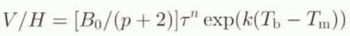
The “deformation velocity” v(z) is a function of the height above ice bottom z. It is related to temperature Τ(z) and basal shear stress τ(z) through (Vialov, 1958)

(2)

T _m is the melting temperature at the bottom of the ice sheet (T _m = 273 − H/1503, where Τ _m is expressed in Κ) and R, is the gas constant, τ_e is the effective stress and τ_xz is the shear stress, namely τ = ρɡΗα, where ρ is the ice density, ɡ is the acceleration of gravity and α is the surface slope in the flowline direction. In the shallow-ice approximation, the other stress components are neglected and τ_e = τ. To smooth the effect of longitudinal stresses due to the irregular bedrock topography, the shear stress is calculated over a distance of the order of 50 km (Young and others, 1989). We also avoid domes and coastal regions where shear stress may not dominate. Equation (2) will be numerically integrated but the analytical expression of Lliboutry (1981) will also be used for qualitative analysis. This stales that

(3)

where V is the averaged deformation velocity of the ice column (V = U (Equation (1)), if there is no sliding), is the mean bottom temperature averaged over the first 5% of the bottom ice (which corresponds to about the first hundred metres); G ₀ is the bottom temperature gradient, taken as 0.022°Cm⁻¹ corresponding to a 50mWm⁻² geothermic flux, while G _d is a flux introduced to take into account the energy dissipation, G _d = Uτ_b (Lliboutry, 1987). Equation (3) is not valid if T _b reaches the melting temperature. Furthermore, because the (p + 2) term takes into account the basal gradient temperature. B ₀ remains independent of ice-column characteristics. If the rheological parameters are constant within the column, then the correlation coefficient between mean velocity from Equation (3) and mean velocity from a numerical integration of Equation (2) is 0.95. The bottom temperature must be estimated from the thermodynamic equation (Lliboutry, 1987) which, under the steady-state assumption, reads

(4)

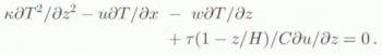
k is the thermal diffusivity, C is the specific heat capacity and w is the vertical velocity. In this equation, we consider vertical diffusion (first term), horizontal advection (second term), vertical advection (third term) and dissipation (last term). More details can be found in Ritz (1987) or Rémy and Minster (1993).

For the whole sector, we then compute U, τ and T _b, which are mapped in figure 2a, b and c; this yields 13 500 data points. The mean velocity map displays the expected behaviour with values increasing from dome to coast. One can observe high local anomalies in the convergence zone (e.g. 72° S, 110° E) or weak local anomalies in the divergence zone (74° S or 77° S, 150° E), which shows the importance of taking convergence or divergence of the flow lines into account (Equation (1)). The shear stress also shows well-known features: it is less than 0.2 bar near domes or ice divides and increases downslope to 1 bar. It also shows local anomalies such as low values at the Vostok “lake” (76–78° S, 105° E) or the Astrolabe “lake” (70° S, 137° E), and high values at 135° E, for instance, which corresponds to well-identified bedrock features (Drewry, 1983) (see Fig. 2d). The basal temperature map looks like the one in Huybrechts (1990): values are close to the melting point, either inside the continent (e.g. Dome C) where vertical advection is weak, or near the coast where dissipation is important.

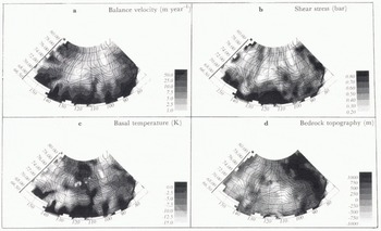
Fig. 2. Maps of balance velocity (a), basal shear stress (b), basal temperature (c) and bedrock topography (d), in the 70–160° E sector.

III. Behaviour of Geophysical Parameters

a. Observations

To first order, Equation (3) shows that the parameter X ^{(V/H)(p + 2)} is only related to the basal values of τ and T _b. One can thus compute the average X0(τ_b0, τ₀) for all the data whose T _b, and τ are equal to T _b0 and τ₀. Numerically, T _b0 is sampled in degree bins, whereas τ₀ is sampled by bins of size 0.05 bar. We expect X0(T _b0, τ₀) to be noisy because we ignore the whole vertical profile contribution. Nevertheless, it should be representative of a given pair (τ_b0, τ₀) to first order. For the whole data set, we can then map the ratio between the observed local value and the averaged one. X(T _b, τ)/X0(T _b, τ) (Fig. 3a). This ratio should be seen as an anomaly of X with respect to the local values of T _b and τ. A strong signal of amplitude ɓ is displayed, meaning that some areas with the same basal temperature and stress can be given values of X different by a factor of ɓ. This has already been observed by McIntyre (1983). It cannot be due to bad sampling; indeed, if the pair (T _b, τ) is unique, the ratio will be equal to 1. Note also that even if n, Q or B>₀ vary with τ or T _b, the same pair will give the same X. Such a strong signal cannot be due to uncertainty on the stress or temperature computation, nor can it be due to the assumptions used to derive Equation (3). Indeed, a factor ɓ should be due either to a very strong error of 18°C in T _b, (if Q = 6 kJ mol⁻¹) or of 0.4 bar in stress (if τ = 0.5 and n = 3), and this is not realistic. This signal is thus really significant.

The same analysis scheme is applied to the shear stress. The difference between the local stress and the average shear stress corresponding to the local values of X and T _b is displayed on figure 3b. The differences may reach 0.25 bar and are thus significant. The most remarkable pattern is the alternation of positive and negative bands in the across direction of the ice flow, suggesting that the longitudinal stress gradient is still present.

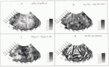
Fig. 3. Maps of the X(T _b, τ)/X0(T _b, τ) ratio (a), of the τ ₀(X, T _b) difference (b), and of the T _b(X, τ) −T _b0(X, τ) difference (c), and of the horizontal stress gradient (d). At the first order, the existence of a flow law should ensure a link between X, τ and T _b. These maps display the geographical anomalies of each parameter. Note that X mostly shows a large-scale signal, while τ shows local across-slops anomalies.

Finally, the same scheme is also applied to temperature. In figure 3c, the pattern looks like the T _b, pattern (Fig. 2c): this means that for a given (X, τ) any value of T _b, can be found; the averaged value is neither significant nor representative of a given (X, τ). First, temperature profiles are mostly controlled by other parameters: for instance, as already mentioned, warm temperatures can be found both in the central part where vertical advection is weak and in the coastal regions where dissipation is important. Secondly, the velocity and the X dependence on temperature is relatively weak: for n = 3 and τ = 0.5 bar (a typical mean value), a stress variation of 0.1 bar leads to a change by a factor of 2 in the estimate of the velocity, whereas the temperature must vary by 6°C to produce the same effect for a 60 kJ mol⁻¹ activation energy. The great sensitivity on the stress component decreases the temperature effect. As a consequence, temperature does not play an important numerical role, as already suggested by Young and others (1989).

IV. Behaviour of Rheological Parameters

a. Estimation of temperature-dependence

Equation (3) can also be written as

(5)

where T _b includes T _m (T _b = T _b – T _m). The large density of data allows us to sample the temperature variable at a 1° rate. We then get from 800 to 1000 data points for each basal-temperature sample from 0° to –10°C and around 500 data points for each colder temperature sample. Moreover, the stress values arc well distributed at each temperature level. For each T _b0, value, one can calculate n(T _b0) and ln(B ₀) + kT _b0 using a linear regression. Both values exhibit a temperature-dependence (Fig. 4). lnB ₀ + kT _b0 increases lineally with basal temperature T _b0; the linear regression coefficient is 0.115, leading to k = 0.115 or to a 70 kJ mol⁻¹ activation energy, as already found by Rémy and Minster (1993); this corresponds to the classical value used in models. Note that B ₀ and Q may vary together, leading to a more complex temperature function but Figure 4 suggests that the variations are roughly compensated. The index n also varies with temperature; it is around 1 for temperatures lower than −10°C and increases with temperature.

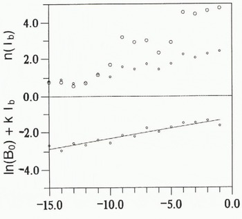
Fig. 4. Glen exponent n value and ln(B ₀) + kT _b, value with respect to basal temperature. Small points are directly obtained from regression of Equation (5). The linear behaviour ln(B ₀) + kT _b suggests that B ₀ and k or Q are constant with temperature. The fitted straight line then gives k = 0.11 or Q = 70 kJ mol⁻¹; the open circles are obtained by integrating Equation (2) and assuming B ₀ and Q constant.

If n varies with temperature, Lliboutry’s (1981) analytical expression (Equation (3)) may be unsatisfactory and Equation (2) must then be numerically integrated. By looking at Figure 4, one can assume that n ≈ 1 for temperatures colder than −10°C and that B ₀ and Q are constant. Because the basal temperature is the warmest one in the column, we selected data points from increasing basal temperature, at a 1° rate. We then looked for the best fit for n(T), sample by sample, from the colder basal-temperature sample to the warmer one. The new n(t) values increase to 3 for temperatures from −10° to −4°C and up to 4.5 for warmer temperatures (see Fig. 4), These values are in good agreement with other estimations (see point 2 of the introduction).

b. Behaviour of rheological parameters against the X large-scale signal

In order to understand the origin of the large-scale signal and/or its effect on the retrieval of the rheological parameters, we separate tbe data set into two sub-sets defined by X(T _b, τ)/X0(T _b, τ) > 1 or < 1; then we look for the behaviour of Equation (5) with temperature. Variations of n and k values (k is tbe slope of the term ln(B ₀) + kT _b) with temperature are identical for the two sub-sets, whereas B ₀) (the constant term of ln(B ₀) + kT _b) values differ by a factor of 3 (Fig. 5). This suggests that the retrieval of n and k (or Q) is not affected by this large-scale signal. This also suggests that the X large-scale trend is mostly due to variation of the pre-exponential factor B ₀ (see point 3 of the introduction). As a matter of fact, a significant signal of longitudinal stress would affect the estimation of the Glen exponent because the effective shear stress includes both the shear stress and the longitudinal stress. In the same way, a significant non-steady-state signal or a wrong temperature calculation would affect the estimate of Q.

Fig. 5. The same as Figure 4 for X(T _b, τ)/X0(T _b, τ) > 1 (small open circles) or < 1 (large open circles), n and k are identical: this suggests that the X large-scale signal (Fig. 2a) is related B ₀ variations, and that n and k retrieval is not affected by this signal.

Conclusion

From the very accurate surface topography of the Antarctic ice sheet deduced from inversion of ERS-1 altimeter data, we can determine the ice-flow direction, the balance velocity and the basal shear stress. The Vialov (1958) equation and Lliboutry’s (1981) assumption yield a relation linking the three following geophysical parameters: (V/H)(p + 2) (where p includes ice-column characteristics and temperature profile), shear stress τ and basal temperature T _b. If one assumes that the rheological parameters n, Q and B ₀ only vary with one of these three geophysical parameters, this relation allows us to map the behaviour anomalies of each geophysical parameter.

Several medium-scale anomalies affect the shear-stress map. The medium-scale anomalies are mostly explained by the longitudinal stress, which can be due either to sliding or bedrock presence and which shows effects on a 100–200 km scale. This longitudinal stress must then be taken into account in the ice-flow modelling.

A strong large-scale anomaly is observed in (V/H)(p + 2): ii seems to be mostly due to a variation in B ₀ but it certainly is partially affected by the poor knowledge of the geothermal flux and by the large-scale longitudinal stress signal.

Finally, one can show that the Glen exponent increases from 1 for temperature below −10°C to 3–4 for higher temperatures. The behaviour of the Arrhenius relation with respect to temperature suggests that the values of B ₀ and of Q (Q = 70 kJ mol⁻¹) do not depend on temperature.

The above results obtained with the help of the first global and accurate surface topography of Antarctica prove the power of the approach. A next step should be the direct assimilation of altimetric data into ice-flow models.