2.1. General description

Let us consider a forced linear dynamical system

(2.1)\begin{equation} \dot{\boldsymbol{x}}={\boldsymbol{\mathsf{A}}}\,\boldsymbol{x}+\boldsymbol{f}, \end{equation}

where the dot denotes time differentiation, $\boldsymbol {x}\in \mathbb {C}^n$ is the state vector, ${\boldsymbol{\mathsf{A}}} \in \mathbb {C}^{n\times n}$ is the linear dynamics matrix and $\boldsymbol {f}\in \mathbb {C}^n$ is an external driving force. Such a system may arise from a semi-discretized partial differential equation, and in the case of fluid flows, the incompressible Navier–Stokes equations can be written in this form by projecting the velocity field onto a divergence-free basis to eliminate the pressure variable. The state $\boldsymbol {x}$ may either represent the deviation from a steady state of a laminar flow, or fluctuations about the temporal mean of a statistically stationary unsteady flow. In both cases the matrix ${\boldsymbol{\mathsf{A}}}$ is the linearization of the underlying nonlinear system about the corresponding base flow, either the equilibrium or the mean. However, if we are dealing with an unsteady flow, it is important to note that a Reynolds decomposition yields a nonlinear term that typically cannot be neglected. In this scenario, the nonlinearity is lumped into $\boldsymbol {f}$ and considered as an external forcing, with the caveat that the system may exhibit preferred input directions due to internal feedback between linear amplification and nonlinear interactions (McKeon & Sharma Reference McKeon and Sharma2010; Beneddine et al. Reference Beneddine, Sipp, Arnault, Dandois and Lesshafft2016).

In this work, we focus on the case where $\boldsymbol {x}$ is the deviation from a stable steady state and $\boldsymbol {f}$ is an exogenous input with no preferential direction, representing disturbances from the environment, model discrepancy, or an open-loop control actuation. For a harmonic forcing ${\boldsymbol {f}(t) = \hat {\boldsymbol {f}}\ \textrm {e}^{-\mathrm {i}\omega t} +\text {c.c.}}$, where $\text {c.c.}$ means complex conjugate, $\omega \in \mathbb {R}$ is the angular driving frequency and $t\in \mathbb {R}$ the time variable, the long-term response is also harmonic, $\boldsymbol {x}(t) = \hat {\boldsymbol {x}}\ \textrm {e}^{-\mathrm {i}\omega t} +\text {c.c.}$, and is governed by the particular solution to (2.1) given by

(2.2)\begin{equation} \hat{\boldsymbol{x}} = \left(-\mathrm{i}\omega{\boldsymbol{\mathsf{I}}}-{\boldsymbol{\mathsf{A}}}\right)^{{-}1}\hat{\boldsymbol{f}}, \end{equation}

where ${\boldsymbol{\mathsf{I}}}$ is the $n\times n$ identity matrix. Let ${\boldsymbol{\mathsf{H}}}(\omega )=(-\mathrm {i}\omega {\boldsymbol{\mathsf{I}}}-{\boldsymbol{\mathsf{A}}})^{-1}$ be the matrix approximation of the resolvent operator, where the negative sign accompanying the $\omega$-term follows the convention used for travelling waves. We seek the largest input–output gain, $\sigma _1(\omega )$, optimized over all possible forcing vectors $\hat {\boldsymbol {f}}$, or more formally

(2.3)\begin{equation} \sigma_1(\omega)= \max_{\hat{\boldsymbol{f}}\ne\boldsymbol{0}}\frac{\| \hat{\boldsymbol{x}}\|^2_{{\boldsymbol{\mathsf{Q}}}}}{\|\,\hat{\boldsymbol{f}}\|^2_{{\boldsymbol{\mathsf{Q}}}}}= \max_{\hat{\boldsymbol{f}}\ne\boldsymbol{0}}\frac{\| {\boldsymbol{\mathsf{H}}}(\omega)\hat{\boldsymbol{f}}\|^2_{{\boldsymbol{\mathsf{Q}}}}}{\|\,\hat{\boldsymbol{f}}\|^2_{{\boldsymbol{\mathsf{Q}}}}},\end{equation}

where $\| \hat {\boldsymbol {x}} \|^2_{\boldsymbol{\mathsf{Q}}}=\hat {\boldsymbol {x}}^*{\boldsymbol{\mathsf{Q}}}\hat {\boldsymbol {x}}$, with $(\ )^*$ denoting the Hermitian transpose, measures the size of the state based on a physically meaningful metric given by the positive–definite weighting matrix ${\boldsymbol{\mathsf{Q}}}$. This weighting accounts for integration quadratures, non-uniform spatial discretizations and appropriate scaling of heterogeneous variables in multi-physics systems (Herrmann et al. Reference Herrmann, Calderón-Muñoz, Diaz and Soto2018a). The Cholesky decomposition is used to factorize ${\boldsymbol{\mathsf{Q}}}={\boldsymbol{\mathsf{F}}}^*{\boldsymbol{\mathsf{F}}}$ and relate the physically relevant norm to the standard Euclidean $2$-norm via $\| \hat {\boldsymbol {x}} \|^2_{{\boldsymbol{\mathsf{Q}}}}=\| {\boldsymbol{\mathsf{F}}}\hat {\boldsymbol {x}} \|^2_2$. With this scaling of the states, and using the definition of the vector-induced matrix norm, the optimal gain optimization problem (2.3) is equivalent to

(2.4)\begin{equation} \sigma_1(\omega)=\| {\boldsymbol{\mathsf{F}}}{\boldsymbol{\mathsf{H}}}(\omega){\boldsymbol{\mathsf{F}}}^{{-}1}\|^2_2.\end{equation}

The solution to (2.4), along with a hierarchy of optimal and sub-optimal forcing and response vectors, is given by the singular value decomposition (SVD) of the weighted resolvent

(2.5)\begin{equation} {\boldsymbol{\mathsf{F}}}{\boldsymbol{\mathsf{H}}}(\omega){\boldsymbol{\mathsf{F}}}^{{-}1}=\boldsymbol{\varPsi}_{{\boldsymbol{\mathsf{F}}}}(\omega) \boldsymbol{\varSigma}(\omega)\boldsymbol{\varPhi}_{{\boldsymbol{\mathsf{F}}}}^*(\omega),\end{equation}

where $\boldsymbol {\varSigma } \in \mathbb {R}^n$ is a diagonal matrix containing the gains $\sigma _1 \geq \sigma _2 \geq \cdots \geq \sigma _n \geq 0$, also known as singular values, and $\boldsymbol {\varPhi }_{{\boldsymbol{\mathsf{F}}}}={\boldsymbol{\mathsf{F}}}\ [\boldsymbol {\phi }_1\ \boldsymbol {\phi }_2 \cdots \boldsymbol {\phi }_n]\in \mathbb {C}^{n\times n}$ and $\boldsymbol {\varPsi }_{{\boldsymbol{\mathsf{F}}}}={\boldsymbol{\mathsf{F}}}[\boldsymbol {\psi }_1 \ \boldsymbol {\psi }_2 \cdots \boldsymbol {\psi }_n]\in \mathbb {C}^{n\times n}$ are unitary matrices whose columns, when left multiplied by ${\boldsymbol{\mathsf{F}}}^{-1}$, yield the input and output resolvent modes, $\boldsymbol {\phi }_j$ and $\boldsymbol {\psi }_j$, respectively.

2.2. Input–output analysis

The more general input–output analysis (Jovanović & Bamieh Reference Jovanović and Bamieh2005; Jovanović Reference Jovanović2021) follows from considering that only measurements of the state $\boldsymbol {y}={\boldsymbol{\mathsf{C}}}\boldsymbol {x}$ are observed, and that the forcing is constrained to be of the form $\boldsymbol {f}={\boldsymbol{\mathsf{B}}}\boldsymbol {u}$, where $\boldsymbol {y} \in \mathbb {C}^{n_y}$ and $\boldsymbol {u} \in \mathbb {C}^{n_u}$. In this framework, the matrices ${\boldsymbol{\mathsf{B}}} \in \mathbb {C}^{n\times n_u}$ and ${\boldsymbol{\mathsf{C}}} \in \mathbb {C}^{n_y\times n}$ restrict the input and output subspaces, allowing the analysis of scenarios where only certain measurements are available (e.g. on a specific region of the spatial domain) and where the possible types of actuation are limited. In this case, the long-term response to harmonic forcing of the measured variables is governed by

(2.6)\begin{equation} \hat{\boldsymbol{y}} = {\boldsymbol{\mathsf{C}}}\left(-\mathrm{i}\omega{\boldsymbol{\mathsf{I}}}-{\boldsymbol{\mathsf{A}}}\right)^{{-}1}{\boldsymbol{\mathsf{B}}}\hat{\boldsymbol{u}}, \end{equation}

where, instead of the resolvent, the transfer function ${\boldsymbol{\mathsf{CH}}}(\omega ){\boldsymbol{\mathsf{B}}}$ governs the amplification of the allowed inputs to produce the observed outputs. The analysis of the latter operator requires introducing norms based on inner products for both the input and output spaces, $\| \hat {\boldsymbol {u}} \|^2_{{\boldsymbol{\mathsf{Q}}}_u}= \hat {\boldsymbol {u}}^*{\boldsymbol{\mathsf{Q}}}_u\hat {\boldsymbol {u}} = \hat {\boldsymbol {u}}^*{\boldsymbol{\mathsf{F}}}^*_u{\boldsymbol{\mathsf{F}}}_u\hat {\boldsymbol {u}} = \| {\boldsymbol{\mathsf{F}}}_u\hat {\boldsymbol {u}} \|^2_2$ and $\| \hat {\boldsymbol {y}} \|^2_{{\boldsymbol{\mathsf{Q}}}_y}= \hat {\boldsymbol {y}}^*{\boldsymbol{\mathsf{Q}}}_y\hat {\boldsymbol {y}} = \hat {\boldsymbol {y}}^*{\boldsymbol{\mathsf{F}}}^*_y{\boldsymbol{\mathsf{F}}}_y\hat {\boldsymbol {y}} = \| {\boldsymbol{\mathsf{F}}}_y\hat {\boldsymbol {y}} \|^2_2$, respectively. Input–output analysis then amounts to taking the SVD of the weighted transfer function

(2.7)\begin{equation} {\boldsymbol{\mathsf{F}}}_y{\boldsymbol{\mathsf{C}}}{\boldsymbol{\mathsf{H}}}(\omega){\boldsymbol{\mathsf{B}}}{\boldsymbol{\mathsf{F}}}_u^{{-}1}=\boldsymbol{\varPsi}_{{\boldsymbol{\mathsf{F}}}_y}(\omega) \boldsymbol{\varSigma}(\omega)\boldsymbol{\varPhi}_{{\boldsymbol{\mathsf{F}}}_u}^*(\omega),\end{equation}

where $\boldsymbol {\varSigma }$ contains the input–output gains in its diagonal, and the input and output modes are given by $\boldsymbol {\varPhi }_u={\boldsymbol{\mathsf{F}}}_u^{-1}\boldsymbol {\varPhi }_{{\boldsymbol{\mathsf{F}}}_u}$ and $\boldsymbol {\varPsi }_y={\boldsymbol{\mathsf{F}}}_y^{-1}\boldsymbol {\varPsi }_{{\boldsymbol{\mathsf{F}}}_y}$, respectively.

3.1. General description

Data-driven resolvent analysis relies on DMD to approximate the eigenvalues and eigenvectors of the underlying dynamical system. Among the many choices of DMD variants, we use the exact DMD approach of Tu et al. (Reference Tu, Rowley, Luchtenburg, Brunton and Kutz2014b). In the absence of forcing, the evolution of measurements of the dynamical system of interest (2.1) is governed by

(3.1)\begin{equation} \boldsymbol{x}_{k+1}=\exp({\boldsymbol{\mathsf{A}}}{\rm \Delta} t)\boldsymbol{x}_k, \end{equation}

where $\boldsymbol {x}_k$ is the measurement at time $t_k=k{\rm \Delta} t$, and ${\rm \Delta} t$ is the sampling time. As in the previous section, let the the weight matrix ${\boldsymbol{\mathsf{Q}}}={\boldsymbol{\mathsf{F}}}^*{\boldsymbol{\mathsf{F}}}$ define a physically meaningful norm to quantify the size of the state vector. The following transformation allows us to work in the $2$-norm framework,

(3.2)\begin{equation} {\boldsymbol{\mathsf{F}}}\boldsymbol{x}_{k+1}={\boldsymbol{\mathsf{F}}}\exp({\boldsymbol{\mathsf{A}}}{\rm \Delta} t){\boldsymbol{\mathsf{F}}}^{{-}1}{\boldsymbol{\mathsf{F}}}\boldsymbol{x}_k=\boldsymbol{\varTheta}{\boldsymbol{\mathsf{F}}}\boldsymbol{x}_k, \end{equation}

where $\boldsymbol {\varTheta }={\boldsymbol{\mathsf{F}}}\exp ({\boldsymbol{\mathsf{A}}}{\rm \Delta} t){\boldsymbol{\mathsf{F}}}^{-1}$ evolves the weighted measurements ${\boldsymbol{\mathsf{F}}}\boldsymbol {x}_k$ one time step into the future. Under this transformation, the adjoint of $\boldsymbol {\varTheta }$ based on the ${\boldsymbol{\mathsf{Q}}}$-norm is equivalent to the Hermitian adjoint. Thus, using the weighted measurements, we can proceed using readily available DMD codes. To begin, we collect snapshots of the state denoted by $\boldsymbol {x}_k^{(j)}$, where the subscript $k\in \lbrace 1, \ldots , m+1\rbrace$ denotes the sample number, and the superscript $j\in \lbrace 1, \ldots , p\rbrace$ denotes different trajectories started from $p \geq 1$ initial conditions. The next step is to assemble the weighted data matrices

(3.3a)\begin{gather} {\boldsymbol{\mathsf{X}}} = {\boldsymbol{\mathsf{F}}}\left[\boldsymbol{x}^{(1)}_1 \ \boldsymbol{x}^{(1)}_2\cdots \boldsymbol{x}^{(1)}_m \ \left| \ \boldsymbol{x}^{(2)}_1 \ \boldsymbol{x}^{(2)}_2\cdots \boldsymbol{x}^{(2)}_m \ \right|\cdots\left| \ \boldsymbol{x}^{(p)}_1 \ \boldsymbol{x}^{(p)}_2\cdots \boldsymbol{x}^{(p)}_m\right], \right. \end{gather}

(3.3b)\begin{gather}{\boldsymbol{\mathsf{Y}}} = {\boldsymbol{\mathsf{F}}}\left[\boldsymbol{x}^{(1)}_2 \ \boldsymbol{x}^{(1)}_3\cdots \boldsymbol{x}^{(1)}_{m+1} \ \left| \ \boldsymbol{x}^{(2)}_2 \ \boldsymbol{x}^{(2)}_3\cdots \boldsymbol{x}^{(2)}_{m+1} \ \right| \cdots \left| \ \boldsymbol{x}^{(p)}_2 \ \boldsymbol{x}^{(p)}_3\cdots \boldsymbol{x}^{(p)}_{m+1}\right], \right. \end{gather}

where ${\boldsymbol{\mathsf{X}}}$ and ${\boldsymbol{\mathsf{Y}}}$ are of size $n\times p m$. Based on these data matrices, the DMD framework with a rank-$r$ truncated SVD yields the matrices ${\boldsymbol{\mathsf{D}}}_r= \text {diag}(\rho _1,\rho _2,\ldots ,\rho _r)\in \mathbb {C}^{r\times r}$ containing the approximated eigenvalues, and ${\boldsymbol{\mathsf{V}}}_{r,{\boldsymbol{\mathsf{F}}}}\in \mathbb {C}^{n\times r}$ and ${\boldsymbol{\mathsf{W}}}_{r,{\boldsymbol{\mathsf{F}}}}\in \mathbb {C}^{n\times r}$, whose columns are the approximated direct and adjoint eigenvectors of the underlying operator $\boldsymbol {\varTheta }$. The reader is referred to the work of Tu et al. (Reference Tu, Rowley, Luchtenburg, Brunton and Kutz2014b) for the derivation of the adjoint DMD modes. These eigenvalues and vectors are related to those corresponding to ${\boldsymbol{\mathsf{A}}}$ via $\lambda _j=\log (\rho _j)/{\rm \Delta} t$, ${\boldsymbol{\mathsf{V}}}_r={\boldsymbol{\mathsf{F}}}^{-1}{\boldsymbol{\mathsf{V}}}_{r,{\boldsymbol{\mathsf{F}}}}$ and ${\boldsymbol{\mathsf{W}}}_r={\boldsymbol{\mathsf{F}}}^{-1}{\boldsymbol{\mathsf{W}}}_{r,{\boldsymbol{\mathsf{F}}}}$. Hence, we obtain $\boldsymbol {\varLambda }_r= \text {diag}(\lambda _1,\lambda _2,\ldots ,\lambda _r)\in \mathbb {C}^{r\times r}$, ${\boldsymbol{\mathsf{V}}}_r= [\boldsymbol {v}_1 \ \boldsymbol {v}_2\cdots \boldsymbol {v}_r]\in \mathbb {C}^{n\times r}$, and ${{\boldsymbol{\mathsf{W}}}_r= [\boldsymbol {w}_1 \ \boldsymbol {w}_2\cdots \boldsymbol {w}_r]\in \mathbb {C}^{n\times r}}$, that satisfy

(3.4a,b)\begin{equation} {\boldsymbol{\mathsf{A}}}{\boldsymbol{\mathsf{V}}}={\boldsymbol{\mathsf{V}}}\boldsymbol{\varLambda},\quad \text{and}\quad {\boldsymbol{\mathsf{A}}}^+{\boldsymbol{\mathsf{W}}}={\boldsymbol{\mathsf{W}}}\boldsymbol{\varLambda}^*, \end{equation}

for an unknown underlying operator ${\boldsymbol{\mathsf{A}}}$, where ${\boldsymbol{\mathsf{A}}}^+={\boldsymbol{\mathsf{Q}}}^{-1}{\boldsymbol{\mathsf{A}}}^*{\boldsymbol{\mathsf{Q}}}$ is its ${\boldsymbol{\mathsf{Q}}}$-norm adjoint. In other words, we use DMD as a data-driven eigendecomposition, which is not surprising considering that its connection to Arnoldi methods and Krylov subspaces has been clear since the origins of the algorithm (Schmid Reference Schmid2010).

Next, we seek an approximation of the resolvent operator built on $\boldsymbol {\varLambda }_r$, ${\boldsymbol{\mathsf{V}}}_r$ and ${\boldsymbol{\mathsf{W}}}_r$. Our approach leverages an operator-based dimensionality reduction technique first used in the context of non-modal stability analysis by Reddy & Henningson (Reference Reddy and Henningson1993). We now return our attention to the forced system (2.1), and consider an eigenvector expansion of $\boldsymbol {x}$ and $\boldsymbol {f}$, as follows

(3.5a,b)\begin{equation} \boldsymbol{x}(t)={\boldsymbol{\mathsf{V}}}_r\boldsymbol{a}(t),\quad \text{and}\quad \boldsymbol{f}(t)={\boldsymbol{\mathsf{V}}}_r\boldsymbol{b}(t), \end{equation}

where $\boldsymbol {a}= [a_1 \ a_2 \cdots a_r]^\textrm {T}\in \mathbb {C}^r$, and $\boldsymbol {b}= [b_1 \ b_2 \cdots b_r]^\textrm {T}\in \mathbb {C}^r$ are the vector of expansion coefficients in eigenvector coordinates. In the work of Reddy & Henningson (Reference Reddy and Henningson1993), ${\boldsymbol{\mathsf{V}}}_r$ are the eigenvectors associated with the first $r$ eigenvalues with largest real part of a known operator ${\boldsymbol{\mathsf{A}}}$, whereas here they are the DMD modes. Substitution of (3.5a,b) in (2.1), and taking the inner product with ${\boldsymbol{\mathsf{W}}}_r$ at both sides yields

(3.6)\begin{equation} \dot{\boldsymbol{a}}=\boldsymbol{\varLambda}_r\boldsymbol{a} + \boldsymbol{b}, \end{equation}

where we have used the bi-orthogonality property between the sets of direct and adjoint eigenvectors, and assumed that they have been normalized such that ${\boldsymbol{\mathsf{W}}}_r^*{\boldsymbol{\mathsf{Q}}}{\boldsymbol{\mathsf{V}}}_r={\boldsymbol{\mathsf{I}}}\in \mathbb {R}^{r\times r}$. Because we are now working in different coordinates, if we want to retain the physical meaning of the norm, we need to adjust our inner product accordingly. The new weighting matrix is derived as $\|\boldsymbol {x}\|_{{\boldsymbol{\mathsf{Q}}}}^2 = \boldsymbol {x}^*{\boldsymbol{\mathsf{Q}}}\boldsymbol {x}=\boldsymbol {a}^*{\boldsymbol{\mathsf{V}}}_r^*{\boldsymbol{\mathsf{Q}}}{\boldsymbol{\mathsf{V}}}_r\boldsymbol {a}=\|\widetilde {{\boldsymbol{\mathsf{F}}}}\boldsymbol {a}\|_2^2$, where we have defined the new matrix $\widetilde {{\boldsymbol{\mathsf{F}}}}\in \mathbb {C}^{r \times r}$ from the Cholesky factorization of ${\boldsymbol{\mathsf{V}}}_r^*{\boldsymbol{\mathsf{Q}}}{\boldsymbol{\mathsf{V}}}_r=\widetilde {{\boldsymbol{\mathsf{F}}}}^*\widetilde {{\boldsymbol{\mathsf{F}}}}$. We are now ready to proceed with the resolvent analysis for the system (3.6). As presented in the previous section, the weighted resolvent modes and gains are obtained from the SVD of

(3.7)\begin{equation} \widetilde{{\boldsymbol{\mathsf{F}}}}(-\mathrm{i}\omega{\boldsymbol{\mathsf{I}}}-\boldsymbol{\varLambda}_r)^{{-}1} \widetilde{{\boldsymbol{\mathsf{F}}}}^{{-}1}=\boldsymbol{\varPsi}_{\widetilde{{\boldsymbol{\mathsf{F}}}}}(\omega) \boldsymbol{\varSigma}(\omega)\boldsymbol{\varPhi}_{\widetilde{{\boldsymbol{\mathsf{F}}}}}^*(\omega).\end{equation}

The final step is to synthesize the resolvent modes in physical coordinates, as follows

(3.8a,b)\begin{equation} \boldsymbol{\varPhi}={\boldsymbol{\mathsf{V}}}_r\widetilde{{\boldsymbol{\mathsf{F}}}}^{{-}1}\boldsymbol{\varPhi}_{\widetilde{{\boldsymbol{\mathsf{F}}}}},\quad \text{and}\quad \boldsymbol{\varPsi}={\boldsymbol{\mathsf{V}}}_r\widetilde{{\boldsymbol{\mathsf{F}}}}^{{-}1}\boldsymbol{\varPsi}_{\widetilde{{\boldsymbol{\mathsf{F}}}}}. \end{equation}

A schematic that summarizes the entire procedure is shown in figure 1. It is worth pointing out that an analogous procedure can be carried out to obtain data-driven transient growth modes, simply by replacing the resolvent operator with the matrix exponential propagator evaluated at a finite time horizon. In addition, notice that the reduced-order resolvent matrix in (3.7) is of size $r\times r$, meaning that its full SVD requires $O(r^3)$ operations instead of $O(n^3)$, and therefore is considerably cheaper to compute. This projection onto the span of the eigenvectors has been successfully used in operator-based non-modal stability analyses to achieve computational speedups of orders of magnitude (Reddy & Henningson Reference Reddy and Henningson1993; Herrmann et al. Reference Herrmann, Calderón-Muñoz and Soto2018b).

3.2. Data-driven input–output analysis

The extension of the above presented method to the input–output framework is quite straightforward if the dataset is composed from full-state measurements. Just as in the operator-based approach, this allows exploration of what the forcing-response dynamics would be like if the inputs and outputs were restricted by the linear mappings $\boldsymbol {y}={\boldsymbol{\mathsf{C}}}\boldsymbol {x}$ and $\boldsymbol {f}={\boldsymbol{\mathsf{B}}}\boldsymbol {u}$. In a similar fashion to (2.7), data-driven input–output analysis follows from the SVD of

(3.9)\begin{equation} {\boldsymbol{\mathsf{F}}}_y{\boldsymbol{\mathsf{CV}}}_r(-\mathrm{i}\omega{\boldsymbol{\mathsf{I}}}-\boldsymbol{\varLambda}_r)^{{-}1}{\boldsymbol{\mathsf{W}}}^*{\boldsymbol{\mathsf{QB}}}{\boldsymbol{\mathsf{F}}}_u^{{-}1}= \boldsymbol{\varPsi}_{{\boldsymbol{\mathsf{F}}}_y}(\omega)\boldsymbol{\varSigma}(\omega)\boldsymbol{\varPhi}_{{\boldsymbol{\mathsf{F}}}_u}^*(\omega),\end{equation}

where, again, $\boldsymbol {\varSigma }$ contains the input–output gains in its diagonal, and the input and output modes are given by $\boldsymbol {\varPhi }_u={\boldsymbol{\mathsf{F}}}_u^{-1}\boldsymbol {\varPhi }_{{\boldsymbol{\mathsf{F}}}_u}$ and $\boldsymbol {\varPsi }_y={\boldsymbol{\mathsf{F}}}_y^{-1}\boldsymbol {\varPsi }_{{\boldsymbol{\mathsf{F}}}_y}$, respectively. In (3.9) we have once more leveraged the projection onto the eigen-basis learned from DMD.

We stress the fact that the presented framework considers full-state measurement data, which are generally required to approximate $\boldsymbol {\varLambda }_r$, ${\boldsymbol{\mathsf{V}}}_r$ and ${\boldsymbol{\mathsf{W}}}_r$. Learning the spectrum and eigenvectors of a linear system from a dataset composed of partial state recordings of the dynamics generated using limited actuation remains an open challenge. This is further discussed in § 5 with our results at hand.

4.1. Complex Ginzburg–Landau equation

Our first example is the linearized complex Ginzburg–Landau equation, which is a typical model for instabilities in spatially evolving flows. The system is governed by the linear operator

(4.1)\begin{equation} {\boldsymbol{\mathsf{A}}} ={-}\nu {\boldsymbol{\mathsf{D}}}_x + \gamma {\boldsymbol{\mathsf{D}}}_x^2 + \mu(x), \end{equation}

where $x$ is the spatial coordinate, and ${\boldsymbol{\mathsf{D}}}_x$ and ${\boldsymbol{\mathsf{D}}}^2_x$ are the first- and second-order spatial differentiation matrices with homogeneous boundary conditions at $x\rightarrow \pm \infty$. We choose a quadratic spatial dependence for the parameter $\mu (x)=(\mu _0-c_{\mu }^2)+({\mu _2}/{2})x^2$, that has been used previously by several authors, e.g. Bagheri et al. (Reference Bagheri, Henningson, Hoepffner and Schmid2009b). The other parameters are set to $\mu _0=0.23$, $\mu _2=-0.01$, $\nu =2+0.4\mathrm {i}$ and $\gamma =1-\mathrm {i}$, giving rise to a linearly stable dynamics. As in Bagheri et al. (Reference Bagheri, Henningson, Hoepffner and Schmid2009b), we use spectral collocation based on Gauss-weighted Hermite polynomials to build the differentiation matrices ${\boldsymbol{\mathsf{D}}}_x$ and ${\boldsymbol{\mathsf{D}}}^2_x$ and the integration quadrature ${\boldsymbol{\mathsf{Q}}}$. The spatial coordinate is discretized into $n=220$ collocation points, and the domain is truncated to $x\in [-85,85]$, which is sufficient to enforce the far-field boundary conditions.

Data are generated from $30$ simulations that are each started from different initial conditions which we choose to be the first $30$ Gauss-weighted Hermite polynomials. We record $m=100$ snapshots that are sampled every ${\rm \Delta} t=0.5$ time units. Data-driven resolvent analysis is performed using snapshot matrices assembled considering measurements from the first trajectory only. Subsequently, the method is applied on snapshot matrices where measurements from the other simulations are sequentially concatenated one by one, to investigate the convergence behaviour in regards to the amount of data required. The ${\boldsymbol{\mathsf{Q}}}$-norm error between the first four operator-based and data-driven resolvent modes as a function of the number of trajectories considered is shown in figures 2(c) and 2(e) for two different input frequencies $\omega _1=0.55$ and $\omega _2=2$, respectively. As more data are included, the abrupt drop in the error is expected, since DMD is able to accurately approximate a larger number of eigenvectors, therefore enriching the basis we use to represent the resolvent modes.

Figure 2.

Data-driven resolvent analysis of the linearized complex Ginzburg–Landau equation. (a) The first four forcing and response modes at $\omega _1=0.55$, where solid and dashed lines show the real part and magnitude of the modes. (b) The same as (a), but for a frequency $\omega _2=2$ where there is much less gain separation. (c) The ${\boldsymbol{\mathsf{Q}}}$-norm error between the operator-based and the data-driven resolvent modes at $\omega _1$ as a function of the number of trajectories $p$ considered in the dataset. (d) Resolvent gain distribution for the first four modes as a function of frequency. (e) The same as (c), but for $\omega _2$. In (a), (b,d), the thick grey lines show operator-based quantities for a ground-truth comparison.

The first four resolvent modes at $\omega _1$ and at $\omega _2$, as well as their gains as a function the input frequency are shown in figures 2(a), 2(b) and 2(d). In this case, the data-driven analysis provides an accurate approximation of the true leading and sub-optimal resolvent modes, even at frequencies where there is a relatively small gain separation, albeit with a larger mode error. We also note that the error in the approximation of the forcing modes is consistently larger than that of the response modes by approximately an order of magnitude. A reason for this may be that, in the case of non-normal systems, the spatial support of the direct eigenvectors is similar to that of the response modes, but it is typically separated from that of the forcing modes. For all results presented in this section, we used $r=24$ for the rank truncation in both DMD and the data-driven eigenbasis ${\boldsymbol{\mathsf{V}}}_r$. Note that caution is needed when retaining more vectors in ${\boldsymbol{\mathsf{V}}}_r$ to not include spurious eigenvectors, which instead of enriching the basis can be detrimental to the performance of the method.

4.2. Transitional channel flow

Our second example is the three-dimensional flow in a plane channel of finite length and depth, and with periodic streamwise and spanwise boundary conditions. The system is governed by the incompressible Navier–Stokes equations, and we consider a Reynolds number ${\textit {Re}}=2000$ based on the channel half-height and the centreline velocity, and a domain size of $2{\rm \pi} \times 2\times 2{\rm \pi}$ dimensionless length units along the $x$, $y$ and $z$ coordinates that indicate the streamwise, wall-normal and spanwise directions, respectively. The state vector in this case is composed of the three-dimensional flow field of disturbances about the base parabolic velocity profile.

In the case of single-wavenumber perturbations, the dynamics is described by the traditional Orr–Sommerfeld and Squire equations (Schmid & Henningson Reference Schmid and Henningson2001). The corresponding linear operator is built using Chebyshev spectral collocation to discretize the wall-normal direction. The Orr–Sommerfeld/Squire operator is then used to compute the operator-based spectrum and the leading resolvent gain of the three-dimensional flow, as shown in figure 1. This is achieved looping over wavenumber combinations that are compatible with the finite channel dimensions, i.e. integers for the current set-up. We consider $N_y=101$ collocation points, and wavenumbers in the range $|\alpha | \le 7$ for the streamwise component, and $|\beta | \le 7$ for the spanwise component. 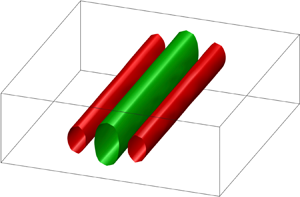The operator-based leading resolvent modes, shown in figure 3, are computed using $\omega =0,\ \alpha =0,\ \beta =2$, for which the maximum gain is observed to occur. The optimal forcing and response correspond to the familiar streamwise vortices that excite streamwise streaks (Trefethen et al. Reference Trefethen, Trefethen, Reddy and Driscoll1993).

Figure 3.

Data-driven resolvent analysis of three-dimensional plane channel flow at ${\textit {Re}}=2000$ based on the channel half-height and the centreline velocity. The method is demonstrated using three datasets obtained from DNS initialized with: (i) small-wavenumber random disturbances, where 15 trajectories are considered, (ii) the optimal forcing and (iii) localized actuation. Operator-based results are also shown for comparison, including the resolvent modes obtained when the input and output are restricted to lie in the span of the snapshots from dataset 3.

To demonstrate our data-driven resolvent analysis, we need snapshots from the transient evolution of the full three-dimensional flow field. We use the spectral code Channelflow (Gibson, Halcrow & Cvitanović Reference Gibson, Halcrow and Cvitanović2008; Gibson Reference Gibson2014) to perform direct numerical simulations of the incompressible Navier–Stokes equations. The code uses Chebyshev and Fourier expansions of the flow field in the wall-normal and horizontal directions, and a third-order Adams–Bashforth backward differentiation scheme for the time integration. We find that a grid with $N_y=65$ and $N_x=N_z=32$ points is sufficient to discretize the domain for the cases studied, and a time step of $0.01$ time units is selected, keeping the Courant–Friedrichs–Lewy (CFL) number at $0.32$. All cases described below are simulated for $400$ time units, and snapshots are saved every ${\rm \Delta} t=0.5$ time units. The perturbation kinetic energy of all initial conditions simulated is set to $10^{-5}$ to ensure that the effect of nonlinearity is negligible.

In order to demonstrate our data-driven method on a higher-dimensional system than in the previous example, rather than Fourier transforming in the streamwise and spanwise directions to perform a separate local analysis for each wavenumber tuple, we directly use the three-dimensional flow field data to perform a global analysis. This provides a more challenging test bed, requiring that we learn a much larger eigen-basis.

First, we consider initial disturbances of the form

(4.2)\begin{equation} \boldsymbol{u}(x,y,z,0)=\sum_{i,j,k,l}\left(c_{ijkl}T_k(y)\exp({\mathrm{i}(ix + jz)}) + \text{c.c.}\right)\textbf{e}_l, \end{equation}

where $i,j\in \lbrace -3, \ldots , 3\rbrace$, $T_k(y)$ are Chebyshev polynomials with $k \in \lbrace 1, \ldots , 65\rbrace$, $l\in \lbrace 1, \ldots , 3\rbrace$, and $c_{ijkl}$ are randomly sampled complex numbers from inside the unit disk. Once generated, the disturbances are corrected to satisfy the boundary and divergence-free conditions, and scaled to have the desired kinetic energy. To investigate the convergence of the method with the amount of data, we consider growing datasets aggregating the snapshots from $1$ up to $15$ simulations initialized with these random small-wavenumber disturbances. The first three forcing and response modes at $\omega =0$ are computed retaining $r=400$ DMD modes and $p=15$ initial conditions, and are shown in figure 4(a). With $r=400$ fixed, as the number of trajectories in the dataset $p$ increases, the ${\boldsymbol{\mathsf{Q}}}$-norm error between data-driven and operator-based resolvent modes slowly decreases, as shown in figure 4(b). To put in perspective the large amount of data used, recall that the state of the system is comprised of the three components of the velocity field at every grid point, yielding a vector of dimension $\sim 2\times 10^5$, and for every trajectory simulated we record $800$ snapshots, resulting in a total of $12\,000$ snapshots for the case with $p=15$. Moreover, considering $p=15$ trajectories, the convergence of the leading and sub-optimal modes with the number of DMD eigenvectors retained $r$ is shown in figure 4(c). It is important to notice that the respective resolvent gains also converge around the same values of $p$ and $r$, as shown in figures 4(b) and 4(c), therefore they could be used as an alternative to assess convergence when the reference modes are not available.

Figure 4.

Convergence of data-driven resolvent modes of three-dimensional plane channel flow at ${\textit {Re}}=2000$ based on the channel half-height and the centreline velocity. (a) The first three forcing and response modes at the dominant frequency $\omega =0$ computed with $r=400$ DMD eigenvectors learned from a dataset composed of $p=15$ simulations initialized with random disturbances of the form shown in (4.2). (b) Data-driven resolvent gains and ${\boldsymbol{\mathsf{Q}}}$-norm error between the operator-based and the data-driven resolvent modes as a function of $p$ with $r=400$. (c) The same, but with $p=15$ fixed, and as a function of $r$ instead. In (b,c) the superscript true denotes the operator-based modes obtained using direct computation of the resolvent.

In addition to how much data are required for the data-driven resolvent discussed above, we now investigate the more interesting question of which data. To do so, we learn the leading resolvent modes, spectra and resolvent gain distributions from three datasets obtained from qualitatively different initial perturbations. The first dataset is the one described above for the convergence study, composed of $p=15$ simulations initialized with random disturbances of the form of (4.2). Data-driven resolvent analysis is applied retaining $r=400$ DMD eigenvectors, and the learned spectrum, gains and modes are shown in figure 3. The data-driven approximation of the optimal gain is very accurate in a narrow band around the optimal frequency $\omega =0$, and closely follows the trend of the operator-based gain distribution over a broad range of frequencies. The quality of the approximation degrades for larger frequencies where the magnitude of the optimal gain decreases.

The second dataset considers a single simulation started using the optimal forcing mode as the initial condition. In this scenario, the optimal gain and modes can be learned with only $r=20$ DMD eigenvectors, as shown in figure 3. It is interesting to look at the DMD eigenvalues, which for this case form a small subset of those learned from the first dataset, as shown in figure 3. In the previous case we learned the eigenvalues with largest real part, now we discover ones from a very specific subset of the complex plane. This highlights that, although the resolvent modes can be accurately represented by very few eigenvectors, the amount of data required to learn those eigenvectors that form an efficient basis is highly dependent on the dynamic trajectories sampled. Moreover, this opens up exciting research directions, emphasizing the importance of finding principled disturbance designs to effectively probe dynamical systems.

Lastly, the third dataset considers a localized disturbance as initial condition, which was previously studied by Ilak & Rowley (Reference Ilak and Rowley2008). The exact form of the wall-normal velocity component is

(4.3)\begin{equation} v(x,y,z,0)=\left(1-\frac{r^2}{c_r^2}\right)\left(\cos({\rm \pi} y) +1\right)\exp{({-}r^2/c_r^2-y^2/c_y^2)}, \end{equation}

where $r^2=(x-{\rm \pi} )^2+(z-{\rm \pi} )^2$, and the parameters are set to $c_r=0.7$ and $c_y=0.6$. This type of disturbance is close to what could be generated in experiments using a spanwise and streamwise periodic array of axisymmetric jets injecting fluid perpendicular to the wall. Data-driven resolvent analysis is performed using $r=200$ DMD eigenvectors, and the resulting optimal forcing and response modes do not resemble the operator-based ones, as shown in figure 3. In this scenario, the true resolvent modes of the system do not lie on the span of the learned DMD eigenvectors. More importantly, this occurs because some of the eigenvectors required to represent the true resolvent modes are not in the span of the data snapshots, and thus cannot be learned by DMD. In fact, we show in figure 3 that the learned resolvent modes for this dataset coincide with the operator-based ones when the input and output subspaces are constrained to lie on the span of the data snapshots.

5.1. Computational cost and memory allocation

As already mentioned in § 3, because of the projection onto the DMD learned eigen-basis, our method builds a reduced-order resolvent operator of size $r\times r$. The subsequent analysis requires taking an SVD with an operation count of up to $O(r^3)$, instead of the $O(n^3)$ operations taxed by the standard matrix-forming operator-based approach, where $n$ is the number of state variables. Although the potential time savings are promising, the computational bottleneck of the presented data-driven method is the truncated SVD in the DMD step, with an operation count of $O(np^2m^2)$, where $p$ is the number of trajectories evolving from different initial conditions and $m$ is the number of snapshots recorded along each of them. This is typically greater than $O(r^3)$, but still lower than $O(n^3)$. For a very high-dimensional system in which many transient trajectories need to be recorded, the memory allocation of the data matrices can also become challenging. For instance, in our channel flow example, dataset 1 considers $12\,000$ snapshots of state vectors with $\sim 2\times 10^5$ entries. Fortunately, our approach benefits from all past and future innovations to improve the accuracy, robustness, flexibility, and speed of DMD (Kutz et al. Reference Kutz, Brunton, Brunton and Proctor2016). In particular, the randomized DMD technique developed by Erichson et al. (Reference Erichson, Mathelin, Kutz and Brunton2019b) may be useful to reduce the computational cost, and the streaming DMD algorithm by Hemati et al. (Reference Hemati, Williams and Rowley2014) can be used to avoid allocating the full data matrices.

5.2. Spatio-temporal resolution

A challenging aspect for the application of our method in an experimental scenario is the requirement of measurements that are spatially and temporally resolved. As in the operator-based approach, an accurate spatial discretization is required, since we need to be able to resolve a large number of DMD modes that conform the basis in which the computed resolvent modes are synthesized. Regarding temporal resolution, the sampling frequency for DMD is lower bounded by the Nyquist criterion, meaning that the signal of interest should be sampled with at least twice its inherent frequency.

It is worth mentioning that there are several extensions and modifications to DMD that may help alleviate these requirements by exploiting low-rank structure and sparsity in the data. If there are only a few dominant modes in the dataset, compressed sensing techniques enable the use of DMD with data that are heavily sub-sampled in space (Brunton et al. Reference Brunton, Proctor, Tu and Kutz2015; Erichson, Brunton & Kutz Reference Erichson, Brunton and Kutz2019a). Moreover, non-uniform sampling in time can be performed at an average rate that is below the Nyquist cutoff, provided that the time dynamics of the dominant modes admits a sparse Fourier representation (Tu et al. Reference Tu, Rowley, Kutz and Shang2014a; Guéniat, Mathelin & Pastur Reference Guéniat, Mathelin and Pastur2015).

However, the sparsity and low-rank assumptions do not typically hold for transient dynamics of non-normal systems, as discussed in the next section. Because of this, we advise caution in the implementation of these DMD extensions to perform data-driven resolvent analysis. In the setting of conventional DMD, a good practice to select the time resolution is sampling the system at approximately three times the Nyquist cutoff (Schmid Reference Schmid2010). A final recommendation is to use a high-order integration quadrature to define the inner-product weighting, which may help alleviate the spatial resolution requirement.

5.3. Non-normality

As highlighted in our results for both examples, an accurate approximation of the resolvent modes requires a dataset composed of several transient trajectories of the system initialized from a large enough set of different initial disturbances to ensure coverage of the dynamical features of the system. However, for highly non-normal systems, enlarging or enriching the dataset may not be enough.

Perhaps the most critical potential pitfall of the application of our method is the intrinsic difficulty to get a numerically robust spectrum in highly non-normal flows (Trefethen & Embree Reference Trefethen and Embree2005). These systems are characterized by eigenvectors that are close to being parallel and are therefore extremely sensitive to perturbations of the dynamics operator (Trefethen & Embree Reference Trefethen and Embree2005; Sipp et al. Reference Sipp, Marquet, Meliga and Barbagallo2010). At the same time, it is well established that, for non-normal flows, individual global modes carry no physical meaning, and only a linear combination of a great many of them yields physically relevant features, such as the resolvent modes (Sipp et al. Reference Sipp, Marquet, Meliga and Barbagallo2010). As a consequence, machine precision may not be enough to accurately compute an eigen-basis that is sufficiently large to reconstruct the dynamics, as shown by Garnaud et al. (Reference Garnaud, Lesshafft, Schmid and Huerre2013) for the case of a two-dimensional jet. Moreover, in unbounded flows that are advection dominated, the introduction of artificial upstream or downstream boundaries to truncate the computational domain may give rise to spurious global modes (Lesshafft Reference Lesshafft2018).

These difficulties translate to an even more challenging approximation of the eigenvalues and eigenvectors of the system via DMD. Further, using an eigen-basis containing spurious vectors to perform data-driven resolvent analysis poses the risk of producing unreliable results. Due to the ubiquity of unbounded and highly non-normal flows, we expect future research to focus on these aspects.

5.4. Nonlinearity

An inherent limitation of the present method is that it is only suitable for systems in a linear regime, i.e. nonlinear systems close to an equilibrium point or actual linear systems. In the case of disturbances close to an equilibrium point, a simple test to ensure that the system is evolving linearly and that use of our method is appropriate, would be checking if DMD is able to reconstruct the recorded dynamics. Further, the extension to nonlinear systems would enable the analysis of statistically stationary turbulent flows provided that the mean-flow linearized operator was inferred from data. However, this requires yet another new method that is capable of distinguishing between the linear and nonlinear dynamics governing the evolution of spatio-temporal measurements, and is therefore outside of the scope of the present work.

5.5. Partial measurements and limited actuation

In an experimental setting, full-state measurements will rarely be available, and most likely we will only have access to measurements in a bounded spatial region and perhaps of only certain state variables. In such a scenario, we cannot expect our data-driven method to infer input–output relations dominated by unobserved variables, but instead it would produce forcing and response modes that are both restricted to the measurement subspace. More formally, if the state is represented in terms of an eigen-basis, the partial measurements can be expressed as $\boldsymbol {y}={\boldsymbol{\mathsf{C}}}\boldsymbol {x}={\boldsymbol{\mathsf{C}}}{\boldsymbol{\mathsf{V}}}_r\boldsymbol {a}$. If this basis contains the minimal set of eigenvectors needed to represent the resolvent modes with a prescribed level of accuracy, then we require that all columns of ${\boldsymbol{\mathsf{V}}}_r$ are in the row space of ${\boldsymbol{\mathsf{C}}}$, otherwise those eigenvectors cannot be learned from the measurements. Therefore, success of data-driven resolvent analysis using partial measurements is possible, but highly case dependent.

Moreover, in an experiment the types of actuation to generate initial disturbances will be limited by hardware. Nevertheless, as shown in our channel flow example with localized forcing (dataset $3$), even though the flow is forced by a specific input, we learn about the response to inputs living in a much larger subspace. Specifically, the learned forcing modes are constrained to the subspace spanned by the whole sequence of data snapshots, whereas the actual impulse corresponds to the first snapshot only. More formally, if initial disturbances are generated by an actuator configuration limited to producing inputs $\boldsymbol {f}={\boldsymbol{\mathsf{B}}}\boldsymbol {u}$, then the learned forcing and response modes are constrained to live in the controllable subspace of the system, rather than just the column space of ${\boldsymbol{\mathsf{B}}}$. This result is very encouraging, demonstrating that we are able to learn a highly amplified, albeit sub-optimal, forcing mode and its corresponding response mode from an experimentally plausible disturbance. Interestingly, this result implies that, with enough measurements, system controllability is a sufficient, although not necessary, condition to guarantee convergence of data-driven results to the operator-based ones from full resolvent analysis.

The limitations described above make it challenging for this method to approximate the forcing and response modes of the full resolvent operator in an experimental setting. However, even with partial measurements and a limited set of initial disturbances, we envisage experimental applications of data-driven resolvent analysis to learn high-gain input–output pairs that, although will not correspond to the optimal forcing and response, may provide valuable ‘and otherwise unavailable’ information to guide controller design in linear non-normal systems.