


1. Introduction
In recent years, organic light-emitting-diode (OLED) displays have become an increasingly important part of the overall display market. In particular, thanks to their superior display quality, specifically their true black state and fast response time compared with liquid crystal displays (LCDs) (see, for example, Chen et al. Reference Chen, Lee, Lin, Chen and Wu2018), OLED displays are now preferred to LCDs for mobile and high-end television applications (see, for example, Lee et al. Reference Lee2018). Currently, the vast majority of OLED displays are manufactured using a vacuum-coating method with a fine metal mask. However, a number of issues, notably the difficulty of precisely controlling the distance between the mask and the display (see, for example, Zhu et al. Reference Zhu, Wang, Zhang, Jin, Li, Wang, Zhang and Yuan2018), limit the size of displays that can be mass-produced using this technique. As a result, there has been considerable interest in avoiding the difficulties associated with the mask by inkjet printing the active materials (dissolved in one or more carrier solvents) directly into small cavities, hereafter referred to as ‘wells’, in the substrate, the solvent thereafter evaporating to leave the desired deposit of active material in the well (see, for example, Shimoda et al. Reference Shimoda, Morii, Seki and Kiguchi2003; Halls Reference Halls2005; Singh et al. Reference Singh, Haverinen, Dhagat and Jabbour2010; Madigan et al. Reference Madigan, Hauf, Barkley, Harjee, Vronsky and Van Slyke2014; Levermore et al. Reference Levermore, Schenk, Tseng, Wang, Heil, Jatsch, Buchholz and Böhm2016; Walker et al. Reference Walker, Leith, Duff, Tan, Tseng, Schenk and Levermore2016). While there is a substantial body of work on the inkjet printing process and, in particular, on the ejection of the droplets from the printheads and the subsequent dynamics of the detached droplets (see, for example, Hoath Reference Hoath2016), far less work has been done on the evolution of the droplets once they have been deposited into the wells. Of particular industrial interest is the period of time between printing taking place and the printed substrate being placed into a drier, during which the solvents evaporate in a diffusion-limited regime. Inkjet printing of droplets into wells also arises in other contexts (such as, for example, the applications in biotechnology described by Marizza, Keller & Boisen Reference Marizza, Keller and Boisen2013).
While there is a large and rapidly growing literature on the dynamics of evaporating droplets on planar substrates (see, for example, the review articles by Larson (Reference Larson2014); Lohse & Zhang (Reference Lohse and Zhang2015); Brutin & Starov (Reference Brutin and Starov2018) and Giorgiutti-Dauphiné & Pauchard (Reference Giorgiutti-Dauphiné and Pauchard2018), and the many references therein), there has been relatively little work on the evaporation of and/or the deposition from a droplet in a well. Not only is this problem directly relevant to the industrial manufacture of OLED displays, but it is also of interest in its own right as a fundamental scientific problem that is key to understanding the many other situations in which evaporating droplets on non-planar substrates occur (such as, for example, the agrochemical spraying of plants that motivated the work of Tredenick et al. Reference Tredenick, Forster, Pethiyagoda, van Leeuwen and McCue2021).
Experimental studies have been undertaken to investigate the evolution of an evaporating droplet in a cuboidal well by van den Doel & van Vliet (Reference van den Doel and van Vliet2001), and in a cylindrical well by Rieger, van den Doel & van Vliet (Reference Rieger, van den Doel and van Vliet2003), Chen, Tseng & Chieng (Reference Chen, Tseng and Chieng2006); Chen, Chieng & Tseng (Reference Chen, Chieng and Tseng2007), Jung et al. (Reference Jung, Kajiya, Yamaue and Doi2009), Kajiya et al. (Reference Kajiya, Kobayashi, Okuzono and Doi2009) and Vlasko-Vlasov et al. (Reference Vlasko-Vlasov, Sulwer, Shevchenko, Parker and Kwok2020). van den Doel & van Vliet (Reference van den Doel and van Vliet2001) and Rieger et al. (Reference Rieger, van den Doel and van Vliet2003) studied the evolution of the free-surface profile of the droplet before it touches the bottom of the well, hereafter referred to as ‘touchdown’, and showed that the volume of the droplet decreases at a rate that is approximately constant in time and proportional to the length of the contact line (rather than the surface area) of the droplet (both of which behaviours are consistent with predictions of a diffusion-limited model such as that presented in the present work). Chen et al. (Reference Chen, Tseng and Chieng2006) investigated evolution after touchdown and found that, at least for the situations they investigated, the new inner contact line that appears at the centre of the well at touchdown recedes at an approximately constant speed (behaviour that is not, in general, either predicted by the mathematical model or seen in the experimental results presented in the present work). Chen et al. (Reference Chen, Chieng and Tseng2007) showed that the wettability properties of the well can have a strong effect on the evolution of the free surface, and hence on the spatial distribution of the final deposit left in the well after a droplet containing suspended particles has completely evaporated. Jung et al. (Reference Jung, Kajiya, Yamaue and Doi2009) studied the evolution of and the final deposit from a droplet of a polymer solution whose contact line is pinned at the lip of the well, and Kajiya et al. (Reference Kajiya, Kobayashi, Okuzono and Doi2009) extended this work to investigate the effect of adding various surfactants to the droplet. More recently, Vlasko-Vlasov et al. (Reference Vlasko-Vlasov, Sulwer, Shevchenko, Parker and Kwok2020) performed a detailed investigation of a final deposit in the form of concentric rings arising from a stick–slip motion of the receding inner contact line.
In addition to these primarily experimental studies, a number of theoretical investigations of the evaporation of a droplet in a well have also been performed. Okuzono, Kobayashi & Doi (Reference Okuzono, Kobayashi and Doi2009) assumed the evaporative flux from the droplet to be spatially uniform and used a thin-film approximation to analyse the evolution of and the final deposit from a two-dimensional droplet in a rectangular well. Subsequently, Eales et al. (Reference Eales, Dartnell, Goddard and Routh2015) used the same approach to investigate the final deposit from an axisymmetric droplet in an axisymmetric (but, in general, non-cylindrical) well. However, both of these works concern droplets of a polymer solution in which gelation (i.e. solidification) effects play a key role, and so touchdown never occurs. Tarasevich et al. (Reference Tarasevich, Vodolazskaya, Isakova and Abdel Latif2009) calculated the radial velocity within an axisymmetric droplet in a cylindrical well for four different evaporative fluxes (slightly confusingly referred to as ‘four different modes of evaporation’). Son (Reference Son2012) and Ahn & Son (Reference Ahn and Son2015) used a sharp-interface level-set method to simulate numerically the impact and evolution of an evaporating droplet in a cylindrical well, and the evolution of an evaporating droplet in both cuboidal and cylindrical wells, respectively. Wang & Fukai (Reference Wang and Fukai2018) used a finite-element method to calculate numerically the evaporative flux from a droplet in a cylindrical well before touchdown. They considered the situation in which the contact line is pinned on the vertical side of the well (rather than at the lip of the well, as it is in the present work), and found that the confining effect of the side of the well can significantly suppress the evaporation in the vicinity of the contact line and lead to a substantial reduction in the total evaporative flux. In related work on non-evaporating droplets, Kant et al. (Reference Kant, Hazel, Dowling, Thompson and Juel2017, Reference Kant, Hazel, Dowling, Thompson and Juel2018) used a combination of experimental and analytical methods to analyse the spreading of both a single droplet and a sequence of partially overlapping droplets in a ‘stadium-shaped’ well, while Zhang et al. (Reference Zhang, Ku, Cheng, Song and Zhang2018) used the lattice Boltzmann method to simulate numerically the impact and evolution of a droplet in a cuboidal well.
Thus, while there have been previous investigations of various aspects of the evaporation of a droplet in a well, there is still neither a complete mathematical model for this problem nor a comprehensive set of experimental results against which the predictions of such a model can be validated. The aim of the present work is to rectify these omissions. Specifically, the outline of the remainder of the present work is as follows. Firstly, in §§ 2–4 we formulate and analyse a mathematical model for the evolution of a thin droplet in a shallow axisymmetric well of rather general shape both before and after touchdown that accounts for the spatially non-uniform evaporation of the fluid. Secondly, in §§ 5 and 6 we perform physical experiments using three cylindrical wells with different small aspect ratios. Thirdly, in §§ 7 and 8 we validate the mathematical model by comparing the present experimental results and experimental results obtained by previous authors, respectively, with the corresponding theoretical predictions for a cylindrical well. Finally, in § 9 we summarise our findings and indicate some possible directions for future work.
2. Mathematical model
Consider a droplet of fluid in an axisymmetric well in the otherwise dry planar surface of a substrate undergoing quasi-static diffusion-limited evaporation into a quiescent atmosphere. We refer the description to polar coordinates  $r$,
$r$,  $\phi$,
  $z$ with
  $Oz$ along the axis of the well, perpendicular to the surface of the substrate at
  $z = 0$, as sketched in figure 1. We denote the maximum depth of the well, which occurs at
  $r = 0$, by
  $H_0$, and the radius of its lip by
  $R_0$, so that the lip is located at
  $r = R_0$,
  $z = 0$. We take the droplet to be axisymmetric, and denote its free-surface profile by
  $z = h(r,t)$, where
  $t$ denotes time. The droplet is deposited into the well at
  $t=0$, and thereafter its volume decreases due to evaporation until it has completely evaporated, which occurs at
  $t=t_{lifetime}$, where
  $t_{lifetime}$ is the lifetime of the droplet.
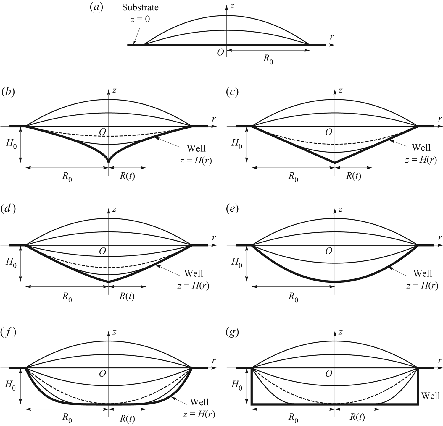
Figure 1. Sketch of snapshots of the free-surface profile  $z=h(r,t)$ of a thin droplet evaporating in a shallow axisymmetric well with profile
  $z = H(r) = - H_0(1 - (r/R_0)^{n})$ in the otherwise dry planar surface
  $z = 0$ of a substrate, for (a) either
  $H_0 = 0$ or
  $n = 0$ (i.e. a planar substrate with no well), (b)
  $0 < n < 1$, (c)
  $n = 1$ (i.e. a conical well), (d)
  $1 < n < 2$, (e)
  $n = 2$ (i.e. a paraboloidal well), (f)
  $2 < n < \infty$ and (g) in the limit
  $n \to \infty$ (i.e. a cylindrical well). In (b–g) the free-surface profile at
  $t=t_{touchdown}$ is indicated with a dashed curve. Note that the dashed curve is not visible in (e) as touchdown occurs everywhere simultaneously within the well in the special case
  $n=2$.
We consider situations in which the droplet is thin and the well is shallow, the droplet is sufficiently small that the effect of gravity is negligible, and the surface tension is sufficiently strong that the free surface of the droplet evolves quasi-statically. More specifically, we consider situations in which the aspect ratio of the droplet and the well,  $\epsilon = H_0/R_0 \ll 1$, is small, as are the appropriately defined Bond number
  ${Bo}$ and capillary number
  ${Ca}$, namely
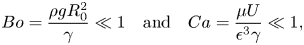 \begin{equation} {Bo} = \frac{\rho g R_0^{2}}{\gamma} \ll 1 \quad \text{and} \quad {Ca} = \frac{\mu U}{\epsilon^{3}\gamma} \ll 1, \end{equation}
where  $\rho$,
  $\gamma$ and
  $\mu$ are the constant density, surface tension and dynamic viscosity of the fluid, respectively,
  $g$ denotes the magnitude of acceleration due to gravity and
  $U$ is an appropriate radial velocity scale (defined in § 7).
The mean curvature of the free surface of the droplet is spatially constant, and so at leading order in the limit  $\epsilon \to 0$ the free-surface profile
  $h$ satisfies
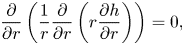 \begin{equation} \frac{\partial}{\partial r}\left(\frac{1}{r}\frac{\partial}{\partial r} \left(r\frac{\partial h}{\partial r}\right)\right) = 0, \end{equation}
and hence takes the general form
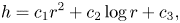 \begin{equation} h = c_1 r^{2} + c_2 \log r + c_3, \end{equation}
where the  $c_i = c_i(t)$ for
  $i = 1$,
  $2$,
$2$,  $3$ are yet to be determined.
We consider a shaped well with profile  $z = H(r)$ (
 $\le 0$), where
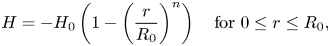 \begin{equation} H ={-} H_0\left(1 - \left(\frac{r}{R_0}\right)^{n}\right) \quad \text{for} \ 0 \le r \le R_0, \end{equation}
in which the exponent  $n$ (
$n$ ( $\ge 0$) is a constant. The volume of the well (i.e. its volume below the plane
  $z = 0$) is given by
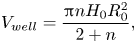 \begin{equation} V_{well} = \frac{{\rm \pi} n H_0 R_0^{2}}{2 + n}, \end{equation}
and any three of the four quantities  $V_{well}$,
  $R_0$,
  $H_0$ and
  $n$ may be prescribed. Cases with either
  $H_0 = 0$ or
  $n = 0$ in (2.4), sketched in figure 1(a), correspond to the familiar case of a droplet on a planar substrate with no well. The cases
  $n = 1$,
  $n = 2$ and in the limit
  $n \to \infty$, also included in figure 1, correspond respectively to a conical well, a paraboloidal well (which will turn out to be an important special case), and a cylindrical well with vertical side
  $r = R_0$ and flat bottom
  $z = -H_0$. The latter case, which, as we have already seen, is of particular interest from a practical point of view, is the subject of the experimental investigation reported in the present work. At its lowest point located at
  $r = 0$,
  $z = -H_0$ the profile of the well (2.4) has a cusp when
  $0 < n < 1$, has a corner when
  $n = 1$, and is flat when
  $n > 1$; also its curvature there is infinite when
  $0 < n < 2$, takes the value
  $4H_0/R_0^{2}$ when
  $n = 2$, and is zero when
  $n > 2$. The slope of the well at its lip is
  $nH_0/R_0$.
We assume that, at least in the first stage of the evolution, the contact line is pinned at the lip of the well located at  $r = R_0$,
  $z = 0$. The initial volume of the droplet,
  $V_0$, could be greater than, equal to, or less than the volume of the well,
  $V_{well}$, in which case the initial free surface of the droplet would be respectively above, at, or below the plane
  $z = 0$. Although all of these cases could be analysed by the present approach, for definiteness we take
  $V_0$ to be greater than
  $V_{well}$, so that initially the well is completely filled and the free surface is above
  $z = 0$.
At some time  $t = t_{touchdown}$ (
 $0 < t_{touchdown} \le t_{lifetime}$) the free surface makes contact tangentially (i.e. at zero contact angle) with the surface of the well. As shown by the dashed curves in figure 1, when
  $0 < n < 2$ touchdown occurs at the lip of the well, and when
  $n > 2$ it occurs at the centre of the well. In the special case n = 2 touchdown occurs everywhere simultaneously within the well, and so the dashed curve is not visible in figure 1(e). Before touchdown the behaviour of the droplet is the same in all three cases, which may therefore be analysed together, but after touchdown the behaviour is different, and it is then convenient to consider the three cases separately.
In the special case  $n = 2$ the droplet has completely evaporated at
  $t = t_{touchdown}$, and so
  $t_{lifetime} = t_{touchdown}$. However, in the general case
  $n \ne 2$ the droplet has not completely evaporated at
  $t = t_{touchdown}$, and the nature of its subsequent evolution depends on whether
  $0 < n < 2$ or
  $n > 2$. When
  $0 < n < 2$ we assume that, as sketched in figure 1(b–d), the contact line de-pins from the lip of the well, and thereafter the contact line recedes (i.e. moves inwards towards the centre of the well) with decreasing radius
  $R = R(t)$ until
  $R(t_{lifetime})=0$, at which time the droplet has completely evaporated. On the other hand, when
  $n > 2$ we assume that, as sketched in figure 1(f,g), a new inner contact line appears at the centre of the well (i.e. at the centre of the droplet, which then becomes annular), and thereafter the inner contact line recedes (i.e. moves outwards towards the lip of the well, where the outer contact line remains pinned) with increasing radius
  $R = R(t)$ until
  $R(t_{lifetime})=R_0$, at which time the droplet has completely evaporated.
In the next two sections we analyse the evolution of the droplet before and after touchdown, respectively.
3. Evolution before touchdown, i.e. for  $0 \le t \le t_{touchdown}$

Before touchdown, i.e. for  $0 \le t \le t_{touchdown}$, the contact line is pinned at the lip of the well, and so the free-surface profile given by (2.3) must satisfy
  $h(R_0,t) = 0$; in addition,
  $h$ must be finite at
  $r = 0$, and is therefore of the familiar paraboloidal form
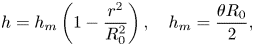 \begin{equation} h = h_{m} \left(1 - \frac{r^{2}}{R_0^{2}}\right), \quad h_{m} = \frac{\theta R_0}{2}, \end{equation}
where  $h_{m} = h_{m}(t) = h(0,t)$ is the height of the free surface at the centre of the well, and
  $\theta = \theta (t) \ll 1$ is the (small) angle that the free surface at the lip of the well makes with the plane
  $z = 0$, i.e.
  $\theta = -\partial h/\partial r$ at
  $r = R_0$. Note that, unlike for a droplet on a planar substrate for which both
  $h_{m}$ and
  $\theta$ must be non-negative, for a droplet in a well they may be positive, zero or negative. The volume
  $V = V(t)$ of the droplet is related to
  $V_{well}$,
  $R_0$,
  $H_0$,
  $n$ and
  $\theta$ by
 \begin{equation} V = V_{well} + \frac{{\rm \pi} \theta R_0^{3}}{4} = \frac{{\rm \pi} n H_0 R_0^{2}}{2 + n} + \frac{{\rm \pi} \theta R_0^{3}}{4}. \end{equation}
 According to the well-known quasi-static diffusion-limited model of the evaporation of a droplet (see, for example, Picknett & Bexon Reference Picknett and Bexon1977; Deegan et al. Reference Deegan, Bakajin, Dupont, Huber, Nagel and Witten1997; Hu & Larson Reference Hu and Larson2002; Popov Reference Popov2005; Dunn et al. Reference Dunn, Wilson, Duffy, David and Sefiane2009; Wray, Duffy & Wilson Reference Wray, Duffy and Wilson2020), the (static) concentration  $c=c(r,z)$ of vapour in the atmosphere satisfies
 \begin{equation} \nabla^{2} c = 0 \quad \text{in} \ z > 0, \end{equation}
with
 \begin{gather} c \to c_{\infty} \quad \text{as} \ r^{2} + z^{2} \to \infty, \end{gather}
 \begin{gather} c = c_{sat} \quad \text{on} \ z = 0 \quad \text{for} \ 0 \le r \le R_0, \end{gather}
 \begin{gather} \frac{\partial c}{\partial z} = 0 \quad \text{on} \ z = 0 \quad \text{for} \ r > R_0, \end{gather}
where  $c_{sat}$ is the constant saturation concentration and
  $c_{\infty } = RHc_{sat}$ is the constant ambient concentration, where
  $RH$
$RH$  $(0 \le RH \le 1)$ is the relative humidity of the vapour in the atmosphere. The local evaporative flux
  $J=J(r)$ from the free surface of the droplet is given by
 \begin{equation} J ={-} D\frac{\partial c}{\partial z} \quad \text{on} \ z = 0 \quad \text{for} \ 0 \le r \le R_0, \end{equation}
where  $D$ is the constant diffusion coefficient of vapour in the atmosphere, and the volume
  $V=V(t)$ evolves according to the global mass-conservation condition
 \begin{equation} \rho \frac{\textrm{d} V}{\textrm{d} t} ={-} 2{\rm \pi}\int_0^{R_0} J \, r \, \textrm{d} r. \end{equation}
Note that, in general, (3.5) and (3.7) apply on the free surface  $z = h$, but for a thin droplet such as that considered in the present work they can be transferred to the plane
  $z = 0$ by Taylor expanding about
  $z = 0$. We denote the initial values of
  $\theta$,
  $h_{m}$ and
  $V$ by
  $\theta _0$,
  $h_{{m}0}$ and
  $V_0$, respectively, so that
 \begin{equation} \theta = \theta_0, \quad h_{m} = h_{{m}0} = \frac{\theta_0 R_0}{2}, \quad V = V_0 = \frac{{\rm \pi} n H_0 R_0^{2}}{2 + n} + \frac{{\rm \pi} \theta_0 R_0^{3}}{4} \quad \text{at} \ t = 0. \end{equation}
Note that for  $0 \le t \le t_{touchdown}$ the concentration
  $c$ and hence the local flux
  $J$ are independent of
  $t$, whereas for
  $t_{touchdown} < t \le t_{lifetime}$ both of them depend on
  $t$ via their dependence on
  $R=R(t)$.
The natural time scale for the evaporation of a thin droplet is  $\rho \theta _0 R_0^{2}/[D(c_{sat}-c_{\infty })]$ (see, for example, Dunn et al. Reference Dunn, Wilson, Duffy, David and Sefiane2008; Schofield et al. Reference Schofield, Wilson, Pritchard and Sefiane2018), and so we non-dimensionalise and scale the variables according to
 \begin{align} \left. \begin{gathered} r = R_0 r^{*}, \quad z = \theta_0 R_0 z^{*}, \quad h = \theta_0 R_0 h^{*}, \quad h_{m} = \theta_0 R_0 h_{m}^{*}, \quad t = \frac{\rho\theta_0 R_0^{2}}{D(c_{sat}-c_{\infty})}t^{*},\\ \theta = \theta_0 \theta^{*}, \quad R = R_0 R^{*}, \quad H = \theta_0 R_0 H^{*}, \quad H_0 = \theta_0 R_0 H_0^{*}, \quad V = \theta_0 R_0^{3} V^{*}, \\ c = c_{\infty}+(c_{sat}-c_{\infty})c^{*},\quad J = \frac{D(c_{sat}-c_{\infty})}{R_0}J^{*}\end{gathered} \right\} \end{align}
for the droplet, and similarly for the atmosphere except that  $z = R_0 \hat {z}$. With the stars and the hat immediately dropped for clarity, (3.1a,b) and (3.2) give
 \begin{equation} h = h_{m} \left(1 - r^{2}\right), \quad h_{m} = \frac{\theta}{2}, \quad V = \frac{{\rm \pi} n H_0}{2 + n} + \frac{{\rm \pi} \theta}{4}, \end{equation}
Laplace's equation (3.3) is unchanged, and (3.4)–(3.9) become
 \begin{gather} c \to 0 \quad \text{as} \ r^{2} + z^{2} \to \infty, \end{gather}
 \begin{gather} c = 1 \quad \text{on} \ z = 0 \quad \text{for} \ 0 \le r \le 1, \end{gather}
 \begin{gather} \frac{\partial c}{\partial z} = 0 \quad \text{on} \ z = 0 \quad \text{for} \ r > 1, \end{gather}
 \begin{gather} J ={-} \frac{\partial c}{\partial z} \quad \text{on} \ z = 0 \quad \text{for} \ 0 \le r \le 1, \end{gather}
 \begin{gather} \frac{\textrm{d} V}{\textrm{d} t} ={-} 2{\rm \pi}\int_0^{1} J \, r \, \textrm{d} r, \end{gather}
 \begin{gather} \theta = 1, \quad h_{m} = \frac{1}{2}, \quad V = \frac{{\rm \pi} n H_0}{2 + n} + \frac{\rm \pi}{4} \quad \text{at} \ t = 0, \end{gather}
respectively. The solution for the concentration  $c$ may be written in the form (see, for example, Fabrikant Reference Fabrikant1995)
 \begin{equation} c = \frac{2}{\rm \pi}\sin^{{-}1} \frac{2}{ [(1 + r)^{2} + z^{2}]^{1/2} + [(1 - r)^{2} + z^{2}]^{1/2} }, \end{equation}
which, using (3.15), leads to the solution for the local flux  $J$, namely
 \begin{equation} J = \frac{2}{{\rm \pi}(1 - r^{2})^{1/2}}, \end{equation}
which exhibits the familiar (integrable) square-root singularity in J at the contact line  $r = 1$ even when the free surface is below the plane
  $z = 0$.
Substituting the expression for  $V$ given by (3.11c) and the expression for
  $J$ given by (3.19) into (3.16) yields
 \begin{equation} \frac{\textrm{d} V}{\textrm{d} t} = \frac{\rm \pi}{4}\frac{\textrm{d} \theta}{\textrm{d} t} ={-}4, \end{equation}
and so the evolution of the droplet before touchdown is given by
 \begin{equation} h = h_{m}(1 - r^{2}), \quad \theta = 1 - \frac{16t}{\rm \pi}, \quad h_{m} = \frac{1}{2} - \frac{8t}{\rm \pi}, \quad V = \frac{{\rm \pi} n H_0}{2 + n} + \frac{\rm \pi}{4} - 4t. \end{equation}
 The free surface is instantaneously flat (i.e.  $\theta = 0$,
  $h_{m} = 0$ and
  $V = V_{well}$) at some time
  $t = t_{flat}$ given by
 \begin{equation} t_{flat} = \frac{\rm \pi}{16} \simeq 0.1963. \end{equation}
As well as being of some interest in its own right, the occurrence of a flat free surface is relatively easy to observe experimentally.
When  $0 < n < 2$ touchdown occurs when
  $\theta = -H'(1) = -n H_0$, where a dash denotes differentiation with respect to argument, showing that
 \begin{equation} t = t_{touchdown} = \frac{{\rm \pi}(1 + n H_0)}{16}, \quad h_{m} ={-}\frac{n H_0}{2}, \quad V = \frac{{\rm \pi} n(2 - n) H_0}{4(2 + n)} \end{equation}
at touchdown. As we have already seen, in the special case  $n = 2$ touchdown occurs everywhere simultaneously within the well, and so
  $t_{lifetime} = t_{touchdown} = {\rm \pi}(1 + 2 H_0)/16$. When
  $n > 2$ touchdown occurs when
  $h_{m} = -H_0$, showing that
 \begin{equation} t = t_{touchdown} = \frac{{\rm \pi}(1 + 2H_0)}{16}, \quad \theta ={-}2H_0, \quad V = \frac{{\rm \pi} (n - 2) H_0}{2(n + 2)} \end{equation}
at touchdown. Setting either  $H_0 = 0$ or
  $n=0$ in (3.23a) or
  $H_0=0$ in (3.24a) gives
  $t_{lifetime} = t_{touchdown} = t_{flat} = {\rm \pi}/16$, recovering the familiar expression for the lifetime of a pinned droplet on a planar substrate (see, for example, Stauber et al. Reference Stauber, Wilson, Duffy and Sefiane2014, Reference Stauber, Wilson, Duffy and Sefiane2015).
4. Evolution after touchdown, i.e. for $t_{touchdown} < t \le t_{lifetime}$

4.1. The case $0 < n < 2$

When  $0 < n < 2$ the free surface touches down at the lip of the well located at
  $r = 1$,
  $z = 0$ at
  $t = t_{touchdown}$, and after touchdown, i.e. for
  $t_{touchdown} < t \le t_{lifetime}$, the non-annular droplet has a receding circular contact line of radius
  $R=R(t)$ which satisfies
  $R(t_{touchdown}) = 1$ and
  $R(t_{lifetime}) = 0$. We must specify a condition in addition to
  $h = H$ at the moving contact line. Since the (paraboloidal) free surface (3.21a) for
  $0 \le t \le t_{touchdown}$ touches down with zero contact angle at
  $r = 1$, we make the natural modelling assumption that the contact angle at the receding contact line remains at the value zero throughout the subsequent evolution. Thus we have the boundary conditions
 \begin{equation} h = H ={-} H_0(1 - R^{n}), \quad \frac{\partial h}{\partial r} = H' = n H_0 R^{n-1} \quad \text{at} \ r = R, \end{equation}
where again a dash denotes differentiation with respect to argument. The solution (2.3) for  $h$ satisfying (4.1) with
  $h$ finite at
  $r = 0$ takes the form
 \begin{equation} h = H(R) - \frac{n H_0 R^{n-2}}{2} \left(R^{2} - r^{2}\right), \end{equation}
or, equivalently,
 \begin{equation} h = h_{m} + \frac{nH_0R^{n-2}r^{2}}{2}, \quad \text{where} \ h_{m} ={-} H_0 + \frac{(2-n)H_0R^{n}}{2}, \end{equation}
for  $0 \le r \le R$, and
  $V$ is given by
 \begin{equation} V = \frac{{\rm \pi} n(2 - n) H_0 R^{2 + n}}{4(2 + n)}. \end{equation}
 The (now quasi-static) concentration  $c=c(r,z,t)$ of vapour in the atmosphere still satisfies Laplace's equation (3.3) and the boundary condition (3.12), but (3.13)–(3.17) must be replaced with
 \begin{gather} c = 1 \quad \text{on} \ z = 0 \quad \text{for} \ 0 \le r \le R, \end{gather}
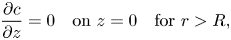 \begin{gather} \frac{\partial c}{\partial z} = 0 \quad \text{on} \ z = 0 \quad \text{for} \ r > R, \end{gather}
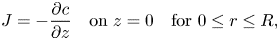 \begin{gather} J ={-} \frac{\partial c}{\partial z} \quad \text{on} \ z = 0 \quad \text{for} \ 0 \le r \le R, \end{gather}
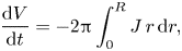 \begin{gather} \frac{\textrm{d} V}{\textrm{d} t} ={-}2{\rm \pi}\int_0^{R} J \, r \, \textrm{d} r, \end{gather}
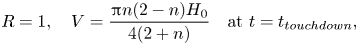 \begin{gather} R = 1, \quad V = \frac{{\rm \pi} n(2 - n) H_0}{4(2 + n)} \quad \text{at} \ t = t_{touchdown}, \end{gather}
respectively, where  $J=J(r,t)$ is again the local evaporative flux. In addition, we have
 \begin{equation} R = 0, \quad V = 0 \quad \text{at} \ t = t_{lifetime}. \end{equation}
As in § 3, for a thin droplet (4.5) and (4.7) are applied on  $z=0$ rather than on
  $z=h$, and similarly for a shallow well (4.6) for
  $R < r \le 1$ is also applied on
  $z=0$ rather than on
  $z=H$. The solution for the concentration
  $c$ of the problem defined by (3.3), (3.12), (4.5) and (4.6) is analogous to (3.18) and is given by
 \begin{equation} c = \frac{2}{\rm \pi}\sin^{{-}1} \frac{2R}{ [(R + r)^{2} + z^{2}]^{1/2} + [(R - r)^{2} + z^{2}]^{1/2} }, \end{equation}
which, using (4.7), leads to the solution for the local flux  $J$ analogous to (3.19), namely
 \begin{equation} J = \frac{2}{{\rm \pi}(R^{2} - r^{2})^{1/2}}. \end{equation}
Substituting (4.4) and (4.12) into (4.8) yields
 \begin{equation} R^{n} \frac{\textrm{d} R}{\textrm{d} t} ={-}\frac{16}{{\rm \pi} n(2 - n)H_0}, \end{equation}
leading to an explicit solution for  $R$ after touchdown, namely
 \begin{equation} R = \left[\frac{1}{n(2 - n)H_0}\left(1 + n + 3n H_0 - \frac{16(1 + n)t}{\rm \pi}\right)\right]^{1/(1 + n)}, \end{equation}
with  $h$ given by (4.2) and
  $V$ given by (4.4), i.e.
 \begin{equation} V = \frac{\rm \pi}{4(2 + n)\left[n(2 - n)H_0\right]^{1/(1 + n)}} \left(1 + n + 3n H_0 - \frac{16(1 + n)t}{\rm \pi}\right)^{(2 + n)/(1 + n)}. \end{equation}
 Figure 2 shows the evolution of the free-surface profile  $h$ for
  $n = 1$ and
  $n = 2$ with
  $H_0 = 1$. Figure 3 shows plots of
  $R$ and
  $V$ as functions of
  $t$ for a range of values of
  $n$, again with
  $H_0 = 1$. Note that
  $\textrm {d} R/\textrm {d} t \to \infty$ and (although not very easy to see in figure 3b)
  $\textrm {d} V/\textrm {d} t \to 0^{+}$ in the limit
  $t \to t_{lifetime}^{-}$.
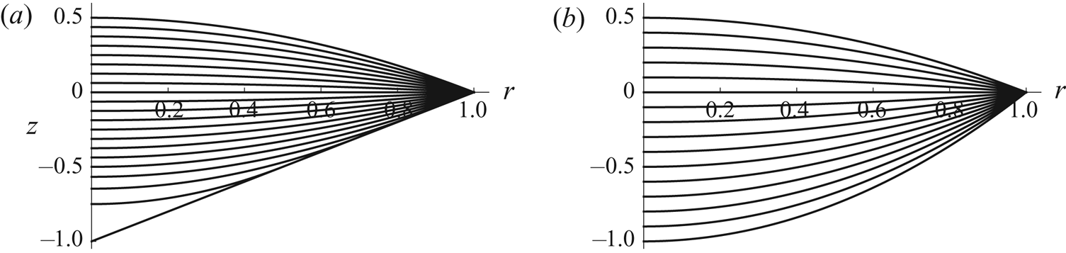
Figure 2. Evolution of the free-surface profile  $h$ given by (3.21a) for
  $0 \le t \le t_{touchdown}$ and by (4.2) for
  $t_{touchdown} < t \le t_{lifetime}$ for (a) a conical well with
  $n = 1$ and
  $H_0 = 1$, and (b) a paraboloidal well with
  $n = 2$ and
  $H_0 = 1$. In (a) the curves are drawn at intervals of
  $t_{touchdown}/16 = {\rm \pi}/128 \simeq 0.0245$, and the lifetime is
  $t_{lifetime} = 5{\rm \pi} /32 \simeq 0.4909$, while in (b) the curves are drawn at intervals of
  $t_{touchdown}/15 = {\rm \pi}/80 \simeq 0.0393$, and the lifetime is
  $t_{lifetime} = t_{touchdown} = 3{\rm \pi} /16 \simeq 0.5890$.
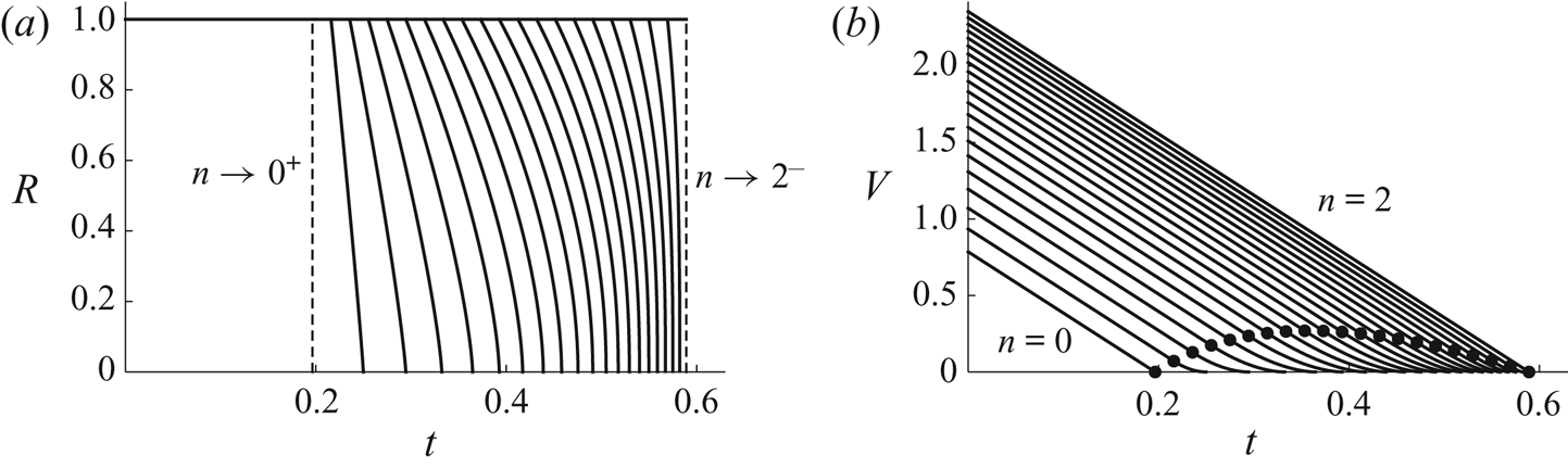
Figure 3. Plots of (a) the radius  $R$ of the receding contact line given by (4.14), and (b) the volume
  $V$ of the droplet given by (3.21d) for
  $0 \le t \le t_{touchdown}$ and by (4.15) for
  $t_{touchdown} < t \le t_{lifetime}$ as functions of
  $t$ for
  $n = 0$,
  $1/10$,
  $1/5$, …,
  $2$ in the case
  $H_0 = 1$. The vertical dashed lines in (a) correspond to the limits
  $n \to 0^{+}$ and
  $n \to 2^{-}$, and the dots in (b) correspond to touchdown (at the lip of the well) at
  $t = t_{touchdown} = {\rm \pi}(1 + nH_0)/16$.
The lifetime of the droplet,  $t_{lifetime}$, which corresponds to
  $R = 0$ and
  $V=0$, is given by
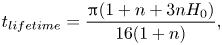 \begin{equation} t_{lifetime} = \frac{{\rm \pi}(1 + n + 3n H_0)}{16(1 + n)}, \end{equation}
which is linear in  $H_0$. Figure 4 includes a plot of
  $t_{lifetime}$ given by (4.16) as a function of
  $n$ for
  $0 \le n \le 2$ (i.e. to the left of the dots) for a range of values of
  $H_0$. For a given value of
  $H_0$, the shortest lifetime is
  ${\rm \pi} /16$, corresponding to
  $n = 0$, and the longest lifetime is
  ${\rm \pi} (1 + 2H_0)/16$, corresponding to
  $n = 2$; also the longest life after touchdown (i.e. the largest value of
  $t_{lifetime} - t_{touchdown}$) is
  $(2 - \sqrt {3}){\rm \pi} H_0/8 \simeq 0.1052 H_0$, corresponding to a well with
  $n = \sqrt {3} - 1 \simeq 0.7321$.
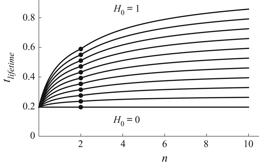
Figure 4. Plot of the lifetime of the droplet,  $t_{lifetime}$, given by (4.16) for
  $0 \le n \le 2$ and by (4.28) for
  $n > 2$, as a function of
  $n$ for
  $H_0 = 0$,
  $1/10$,
  $1/5$, …,
  $1$. The dots denote the values
  $t_{lifetime} = t_{touchdown} = {\rm \pi}(1 + 2 H_0)/16$ for
  $n=2$. The curves approach the asymptotic values
  $t_{lifetime} = {\rm \pi}[1 + 2(1 + 8\alpha _{\infty })H_0]/16 \simeq 0.1963 + 0.8228H_0$ in the limit
  $n \to \infty$.
4.2. The case $n > 2$

When  $n > 2$ the free surface touches down at the centre of the well located at
  $r = 0$,
  $z = -H_0$ at
  $t = t_{touchdown}$, and after touchdown, i.e. for
  $t_{touchdown} < t \le t_{lifetime}$, the annular droplet has a pinned circular outer contact line
  $r=1$ and a receding circular inner contact line of radius
  $R=R(t)$ which satisfies
  $R(t_{touchdown}) = 0$ and
  $R(t_{lifetime}) = 1$. We must again specify a condition in addition to
  $h = H$ at the moving contact line. Since the (paraboloidal) free surface (3.21a) for
 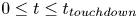 $0 \le t \le t_{touchdown}$ touches down with zero contact angle at
  $r = 0$, we again make the natural modelling assumption that the contact angle at the receding contact line remains at the value zero throughout the subsequent evolution, and so the boundary conditions (4.1) again hold. The solution (2.3) for
  $h$ satisfying (4.1) and
  $h=0$ at
  $r=1$ takes the form
 \begin{equation} h = \frac{H_0\left[\left({-}2R^{2} + nR^{n} - (n - 2)R^{n + 2}\right)\log r - (1 - R^{n} + nR^{n} \log R)(1 - r^{2})\right]} {1 - R^{2} + 2R^{2}\log R}\end{equation}
for  $R \le r \le 1$, and
  $V$ is given by
 \begin{equation} V = {\rm \pi}H_0 f(R), \end{equation}
where we have defined the function  $f = f(R)$ by
 \begin{equation} f = \frac{n \left[4 -(n + 2)R^{n - 2} + (n - 2)R^{n + 2}\right]}{4(n + 2)} - \frac{\left(1 - R^{2}\right)^{2} \left[(n - 2)R^{n} - n R^{n - 2} + 2\right]}{4 \left(1 - R^{2} + 2 R^{2} \log R\right)}. \end{equation}
It is useful to note that  $f \to (n - 2)/[2(n + 2)]$ in the limit
  $R \to 0^{+}$ (in agreement with the expression for
  $V$ at touchdown given by (3.24c)), and that
  $f \sim n^{2}(n - 2)(1 - R)^{4}/36 \to 0^{+}$ in the limit
  $R \to 1^{-}$.
The (again quasi-static) concentration  $c=c(r,z,t)$ of vapour in the atmosphere still satisfies Laplace's equation (3.3) and the boundary condition (3.12), but in this case (3.13)–(3.17) must be replaced with
 \begin{gather} c = 1 \quad \text{on} \ z = 0 \quad \text{for} \ R \le r \le 1, \end{gather}
 \begin{gather} \frac{\partial c}{\partial z} = 0 \quad \text{on} \ z = 0 \quad \text{for} \ 0 \le r < R \quad \text{and} \quad \text{for} \ r > 1, \end{gather}
 \begin{gather} J ={-} \frac{\partial c}{\partial z} \quad \text{on} \ z = 0 \quad \text{for} \ R \le r \le 1. \end{gather}
 \begin{gather} \frac{\textrm{d} V}{\textrm{d} t} ={-}F, \quad \text{where} \ F = 2{\rm \pi}\int_R^{1} J \, r \, \textrm{d} r, \end{gather}
 \begin{gather} R = 0, \quad V = \frac{{\rm \pi} (n - 2) H_0}{2(n + 2)} \quad \text{at} \ t = t_{touchdown}, \end{gather}
respectively, where  $J=J(r,t)$ is again the local evaporative flux, and
  $F=F(R)$ (which depends on
  $t$ via its dependence on
  $R=R(t)$) is the total evaporative flux from the droplet. In addition, we have
 \begin{equation} R = 1, \quad V = 0 \quad \text{at} \ t = t_{lifetime}. \end{equation}
As in § 4.1, (4.20), (4.22) and (4.21) for  $0 \le r < R$ are applied on
  $z = 0$.
Perhaps surprisingly, no simple closed-form solution of the problem for  $c$ defined by (3.3), (3.12), (4.20) and (4.21) is available (see § 10.1.1 of Popov, Hess & Willert Reference Popov, Heß and Willert2019 for an overview of previous work on this problem in the context of contact mechanics). The problem was reformulated as equivalent integral equations by, for example, Cooke (Reference Cooke1963), Williams (Reference Williams1963) and Fabrikant (Reference Fabrikant1993), and the last-mentioned also gave an iteration-based infinite-series solution to their formulation. Since our primary concern is with the total flux
  $F$, we obtained this numerically in two independent ways, namely by solving the integral equation of Cooke (Reference Cooke1963) by means of Chebyshev–Gauss quadrature with typically 200 nodes, and by solving Laplace's equation for
  $c$ using the finite-element package COMSOL Multiphysics 5.3a (COMSOL Inc.), from which
  $J$ and hence
  $F$ were obtained; the values of
  $F$ obtained using these two different approaches were found to be in good agreement.
Figure 5 shows an example of contours of  $c$ in the
  $r$–
$r$– $z$ plane for an annular droplet obtained using COMSOL Multiphysics, figure 6 shows a plot of the local flux
  $J$ from an annular droplet as a function of
  $r$ (
$r$ ( $R \le r \le 1$) for a range of values of
  $R$, as well as that from a non-annular droplet given by (3.19), and figure 7 shows the total flux
  $F$ from an annular droplet as a function of
  $R$ (
$R$ ( $0 \le R \le 1$). Intriguingly, as figure 6 shows, the local flux
  $J$ from a non-annular droplet is smaller than that from an annular droplet with the same outer radius, though, of course, the former is effective over a larger area than the latter (i.e. over
  $0 \le r \le 1$ rather than
  $R \le r \le 1$), and so leads to a larger value of the total flux
  $F$. Figure 6 also shows that
  $J \to \infty$ as
  $r \to R^{+}$ and
  $r \to 1^{-}$, and a local analysis shows that
  $J$ has square-root singularities at both contact lines (i.e. the same singularity as a non-annular droplet). This is true even in the limit
  $R \to 0^{+}$, showing that the local flux
  $J$ due to an annular droplet with a vanishingly small hole at its centre is different from that due to a non-annular droplet (for which
  $J$ is well behaved at
  $r = 0$); the difference is, however, confined to a small region near to
  $r = R \to 0^{+}$ whose contribution to the total flux
  $F$ is small, leading to
  $F \to 4^{-}$ as
  $R \to 0^{+}$, in agreement with the value
  $F = 4$ in the case of a non-annular droplet which appears in (3.20). Note that, as figure 6 shows,
  $J$ is asymmetric about the midpoint
  $(R + 1)/2$ between the contact lines, and, as figure 7 shows,
  $F \to 0^{+}$ as
  $R \to 1^{-}$, i.e. as the width of the annulus approaches zero.
Figure 5. Plot of contours of the concentration  $c$ in the
  $r$–
$r$– $z$ plane for an annular droplet in the case
  $R = 1/2$. The contours are drawn at intervals of
  $0.04$.
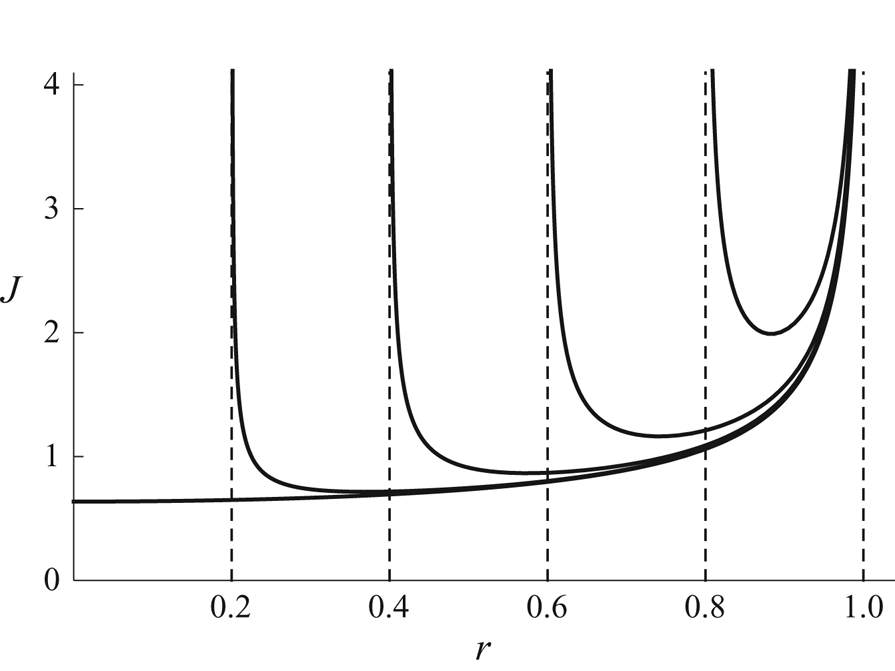
Figure 6. Plot of the local flux  $J$ from an annular droplet as a function of
  $r$ (
$r$ ( $R \le r \le 1$) in the cases
  $R = 0.2$,
  $0.4$,
  $0.6$ and
  $0.8$, as well as that from a non-annular droplet given by (3.19).
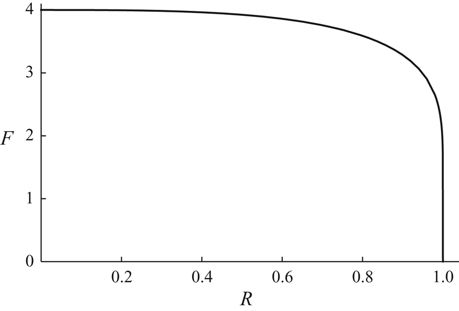
Figure 7. Plot of the total flux  $F$ from an annular droplet as a function of
  $R$ (
$R$ ( $0 \le R \le 1$).
As figure 7 shows, the total flux  $F$ is nearly independent of
  $R$ until
  $R$ gets close to 1, showing that the increase of the perimeter
  $2{\rm \pi} R$ of the receding inner contact line (where
  $J$ is singular), which tends to increase the total flux, almost compensates for the decrease of the surface area
  ${\rm \pi} (1 - R^{2})$ of the annular droplet, which tends to decrease the total flux, for most of the lifetime of the droplet. It is only near to the complete evaporation of the droplet, i.e. when
  $R$ gets close to 1, that
  $F$ rapidly decreases to zero.
With the total flux  $F$ now known, (4.18) and (4.23) give
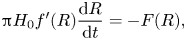 \begin{equation} {\rm \pi}H_0 f'(R) \frac{\textrm{d} R}{\textrm{d} t} ={-} F(R), \end{equation}
where again a dash denotes differentiation with respect to argument, leading to an implicit solution for  $R$ after touchdown, namely
 \begin{equation} t = t_{touchdown} - {\rm \pi}H_0\int_0^{R} \frac{f'(\hat{R})}{F(\hat{R})} \, \textrm{d} \hat{R}, \end{equation}
with  $h$ given by (4.17) and
  $V$ given by (4.18).
Figure 8(a) shows the evolution of the free-surface profile  $h$ for
  $n=9$ with
  $H_0=1$. Figure 9 shows plots of
  $R$ and
  $V$ as functions of
  $t$ for a range of values of
  $n$, again with
  $H_0 = 1$. The nearly linear dependence of
  $V$ on
  $t$ for
  $t_{touchdown} < t \le t_{lifetime}$ evident in figure 9(b) is a consequence of the fact that the total flux
  $F$ is nearly independent of
  $R$ until
  $R$ gets close to 1 discussed above. Note that
  $\textrm {d} R/\textrm {d} t \to \infty$ and (although impossible to see in figure 9b)
  $\textrm {d} V/\textrm {d} t \to 0^{+}$ in the limit
  $t \to t_{lifetime}^{-}$ (i.e. the same behaviour as when
  $0 < n < 2$).
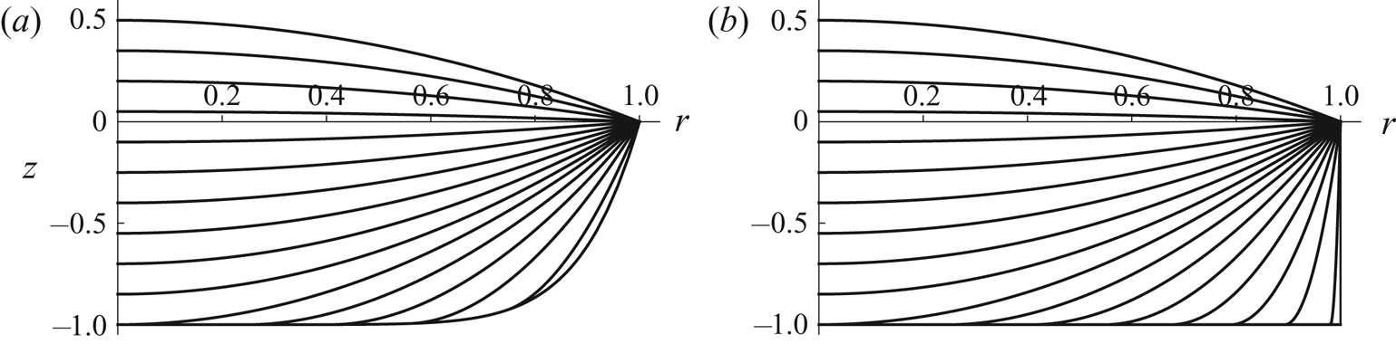
Figure 8. Evolution of the free-surface profile  $h$ given by (3.21a) for
  $0 \le t \le t_{touchdown}$ and by (4.17) for
  $t_{touchdown} < t \le t_{lifetime}$ for (a) a well with
  $n = 9$ and
  $H_0 = 1$, and (b) a cylindrical well (i.e. in the limit
  $n \to \infty$) with
  $H_0 = 1$. In (a) the curves are drawn at intervals of
  $t_{touchdown}/10 \simeq 0.0589$, and the lifetime is
  $t_{lifetime} \simeq 0.8454$, while in (b) the curves are drawn at intervals of
  $t_{touchdown}/10 \simeq 0.0589$, and the lifetime is
  $t_{lifetime} \simeq 1.0193$.
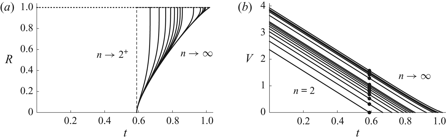
Figure 9. Plots of (a) the radius  $R$ of the receding inner contact line given by (4.27), and (b) the volume
  $V$ of the droplet given by (3.21d) for
  $0 \le t \le t_{touchdown}$ and by (4.18) for
  $t_{touchdown} < t \le t_{lifetime}$ as functions of
  $t$ for
  $n = 2$,
  $3$,
$3$,  $4$, …,
  $10$,
$10$,  $20$,
$20$,  $40$,
$40$,  $60$,
$60$,  $80$ and
  $100$, and in the limit
  $n \to \infty$, in the case
  $H_0 = 1$. The vertical dashed line in (a) corresponds to the limit
  $n \to 2^{+}$, and the dots in (b) correspond to touchdown (at the centre of the well) at
  $t = t_{touchdown} = {\rm \pi}(1 + 2H_0)/16 \simeq 0.5890$.
The lifetime of the droplet, which corresponds to  $R = 1$ and
  $V=0$, is given by
 \begin{equation} t_{lifetime} = t_{touchdown} + {\rm \pi}\alpha H_0 = \frac{\rm \pi}{16}\left[1 + 2\left(1 + 8\alpha\right)H_0\right], \end{equation}
where the function  $\alpha = \alpha (n) \, (\ge 0)$ is given by
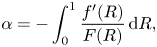 \begin{equation} \alpha ={-}\int_0^{1} \frac{f'(R)}{F(R)} \, \textrm{d} R, \end{equation}
which varies monotonically from  $\alpha = 0$ when
  $n = 2$ to
  $\alpha = \alpha _{\infty } \simeq 0.1369$ in the limit
  $n \to \infty$. Note that, like the corresponding expression for
  $0 < n < 2$ given by (4.16),
  $t_{lifetime}$ given by (4.28) is linear in
  $H_0$. Figure 10 shows a plot of
  $\alpha$ as a function of
  $n$ for
  $n \ge 2$, and figure 4 includes a plot of
  $t_{lifetime}$ given by (4.28) as a function of
  $n$ for
  $n > 2$ (i.e. to the right of the dots) for a range of values of
  $H_0$.
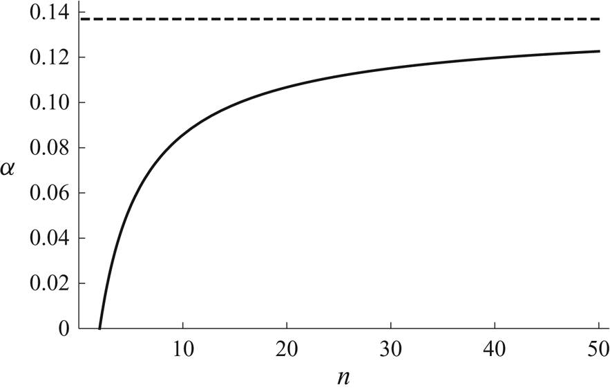
Figure 10. Plot of  $\alpha$ given by (4.29) as a function of
  $n$ for
  $n \ge 2$. The dashed line shows the asymptotic value
  $\alpha = \alpha _{\infty } \simeq 0.1369$ in the limit
  $n \to \infty$.
4.3. The limit $n \to \infty$

In the limit  $n \to \infty$, corresponding to a cylindrical well with vertical side
  $r=1$ and flat bottom
  $z=-H_0$, after touchdown the annular droplet again has a pinned circular outer contact line
  $r=1$ and a receding circular inner contact line
  $r=R$. The solution for
  $h$ given by (4.17) reduces to
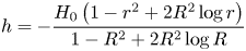 \begin{equation} h ={-}\frac{H_0\left(1 - r^{2} + 2R^{2}\log r\right)}{1 - R^{2} + 2R^{2}\log R}\end{equation}
for  $R \le r \le 1$, and
  $V$ is again given by (4.18), where the function
  $f$ reduces to
 \begin{equation} f = \frac{1 - R^{4} + 4R^{2}\log R}{2\left(1 - R^{2} + 2R^{2}\log R\right)}. \end{equation}
The evolution of the droplet in this limit is as described in § 4.2, with, in particular, the lifetime of the droplet given by (4.28) with  $\alpha = \alpha _{\infty }$, namely
 \begin{equation} t_{lifetime} = \frac{\rm \pi}{16}[1 + 2(1 + 8\alpha_{\infty})H_0] \simeq 0.1963 + 0.8228H_0. \end{equation}
 Figure 8(b) shows the evolution of the free-surface profile  $h$ in the limit
  $n \to \infty$ with
  $H_0=1$.
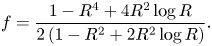
4.4. The critical times $t_{flat}$, $t_{touchdown}$ and $t_{lifetime}$


Figure 11 shows a plot of the critical times  $t_{flat}$, given by (3.22),
  $t_{touchdown}$, given by (3.23a) and (3.24a), and
  $t_{lifetime}$, given by (4.16) and (4.28), as functions of
  $n$ in the case
  $H_0 = 1$. In particular, figure 11 illustrates that
  $t_{flat}$ is independent of
  $n$,
$n$,  $t_{touchdown}$ increases linearly with
  $n$ for
  $0 \le n \le 2$ but is independent of
  $n$ for
  $n > 2$,
  $t_{lifetime}$ increases nonlinearly with
  $n$,
$n$,  $t_{lifetime} = t_{touchdown} = t_{flat} = {\rm \pi}/16$ when
  $n=0$,
  $t_{lifetime} = t_{touchdown} = {\rm \pi}(1 + 2 H_0)/16$ when
  $n=2$, and
  $t_{lifetime} \to {\rm \pi}[1 + 2(1 + 8\alpha _{\infty })H_0]/16$ in the limit
  $n \to \infty$.
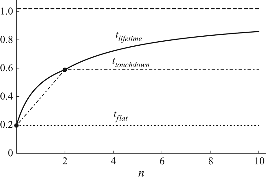
Figure 11. Plot of the critical times  $t_{flat}$, given by (3.22) (dotted line),
  $t_{touchdown}$, given by (3.23a) for
  $0 \le n \le 2$ and by (3.24a) for
  $n > 2$ (dash-dotted line), and
  $t_{lifetime}$, given by (4.16) for
  $0 \le n \le 2$ and by (4.28) for
  $n > 2$ (solid line), as functions of
  $n$ in the case
  $H_0 = 1$. The dashed line shows the asymptotic value
  $t_{lifetime} = {\rm \pi}[1 + 2(1 + 8\alpha _{\infty })H_0]/16 \simeq 1.0191$ in the limit
  $n \to \infty$.
5. Experimental procedure
The experimental procedure employed involved depositing single droplets of the volatile solvent methyl benzoate into shallow axisymmetric cylindrical wells and observing their behaviour as they evaporated. Methyl benzoate is sufficiently volatile that the experiments could be conducted within a reasonable time frame, and its physical properties are consistent with the assumptions of the mathematical model. A schematic diagram of the experimental set-up used is shown in figure 12.
Figure 12. Schematic diagram of the experimental set-up used.
The experiments were carried out under ambient conditions with a relative humidity of methyl benzoate vapour of  $RH = 0$ (and a relative humidity of water vapour of
  $RH = 0.34 \pm 0.10$). The atmospheric pressure was uncontrolled and the ambient temperature was controlled only to within
  $1\,^{\circ }$C of
  $22\,^{\circ }$C. The temperature of the substrate was accurately maintained at
  $22\,^{\circ }$C by means of a proportional-integral-derivative Peltier controller.
The experiments were performed using three shallow wells with radii  $29$
$29$  $\mathrm {\mu }$m,
  $50$
$50$  $\mathrm {\mu }$m and
  $75$
$75$  $\mathrm {\mu }$m and depths
  $2.38$
  $\mathrm {\mu }$m,
  $1.87$
  $\mathrm {\mu }$m and
  $2.39$
  $\mathrm {\mu }$m, respectively. The wells were fabricated in spin-cast films of photo-resist deposited onto glass substrates coated with indium tin oxide (ITO). Further details of the fabrication of the wells are given in Appendix A. Because of the nature of the manufacturing process, the sides of the wells are not perfectly vertical, but, given their small aspect ratios, it is reasonable to regard the wells as being cylindrical for the purpose of comparison with the theoretical predictions of the mathematical model described in §§ 2–4.
Picolitre droplets of methyl benzoate were ejected into the wells from a MicroFab print head (MJABP-01, Microfab Technologies Inc.) with a circular orifice of diameter  $50$
$50$  $\mathrm {\mu }$m under a bipolar waveform generated by a MicroFab controller (JetDrive III CT-M3-02, Microfab Technologies Inc.). The droplet was illuminated from underneath by a cold LED at a wavelength of
  $470$ nm (M470L3, Thorlabs Inc.). The reflected light from the sample was collected by a
  $50\times$ objective lens (TU Plan ELWD, Nikon) with an image resolution of 0.4
  $\mathrm {\mu }$m pixel
 $^{-1}$, and captured through a bandpass filter (bandwidth
  $10 \pm 2$ nm, Thorlabs Inc.) with a high-speed camera (FASTCAM SA4, Photron). The experiments were performed six times for each well to verify the reproducibility of the results.
6. Experimental results
Thin-film interferometry was used to measure the evolution of the free surface of the droplet during its evaporation. Figure 13 shows a typical interferometric pattern observed during the present experiments. In particular, the high degree of axisymmetry shown in figure 13 was found in all of the experiments. Further details of the image-analysis procedure used are given in Appendix B. The initial time,  $t=0$, was arbitrarily chosen to be a time at which well-resolved interference fringes were observed and the contact line of the droplet coincided with the lip of the well (taken to be at the boundary of the outermost bright fringe, as indicated by the circle in figure 13), i.e. no fluid overflow.
Figure 13. A typical interferometric pattern observed during the present experiments. The circle indicates the lip of the well, the cross the centre of the well, and the line the cross-section along which the fringes are analysed.
Table 1 shows experimental values of the radius  $R_0$, the depth H 0 and the aspect ratio
  $\epsilon =H_0/R_0$ of the three wells investigated, together with values of the initial angle
  $\theta _0$ and the initial evaporation rate
  $\left .\textrm {d} V/\textrm {d} t\right \vert _{t=0}$, and the critical times
  $t_{flat}$,
  $t_{touchdown}$ and
  $t_{lifetime}$, for a representative droplet in each well. Note that since the experimental values of the critical times depend on the arbitrarily chosen initial time,
  $t=0$, as well as on the values of the ambient temperature and the atmospheric pressure, we give representative (rather than average) results for each well. We will discuss a parameter-free quantity involving the relative values of the critical times in § 7.
Table 1. Experimental values of the radius  $R_0$, the depth
  $H_0$ and the aspect ratio
  $\epsilon =H_0/R_0$ of the three wells investigated, together with values of the initial angle
  $\theta _0$ and the initial evaporation rate
  $\left .\textrm {d} V/\textrm {d} t\right \vert _{t=0}$, and the critical times
  $t_{flat}$,
  $t_{touchdown}$ and
  $t_{lifetime}$, for a representative droplet in each well.
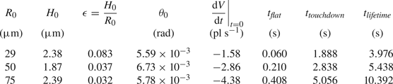
Figure 14 shows experimental results for the free-surface profile  $h$ of a droplet before touchdown and paraboloidal fits to these values as functions of
  $r$ for all three wells at equally spaced times. All of the paraboloidal fits intersect to within
  $\Delta r = \pm 1$
  $\mathrm {\mu }$m and
  $\Delta h = \pm 0.05$
  $\mathrm {\mu }$m of each other, indicating that the contact line of the droplet remains pinned at the lip of the well before touchdown, and the position of the average intersection point was used to determine the radius
  $R_0$ and the depth
  $H_0$ of each well. The initial angle
  $\theta _0$ of the droplet was calculated from the average of the derivatives of the paraboloidal fit to the initial free-surface profile at the lip of the well.
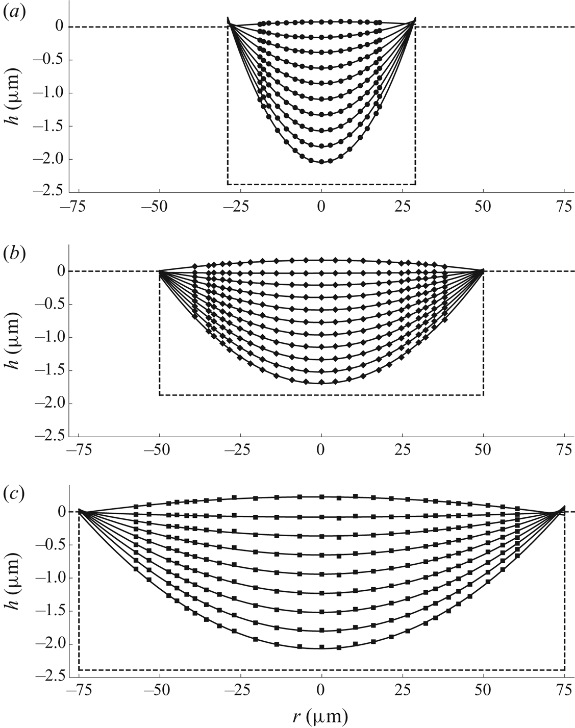
Figure 14. Experimental results for the free-surface profile  $h$ of a droplet before touchdown (symbols) and paraboloidal fits to these values (solid black lines) as functions of
  $r$ for wells of radius
  $29$
$29$  $\mathrm {\mu }$m at times
  $t=0,0.18, \ldots , 1.62$ s,
  $50$
$50$  $\mathrm {\mu }$m at times
  $t=0,0.26, \ldots , 2.34$ s and
  $75$
$75$  $\mathrm {\mu }$m at times
  $t=0,0.56, \ldots , 4.48$ s. The experimental values are denoted by circles, diamonds and squares for the
  $29$
$29$  $\mathrm {\mu }$m,
  $50$
$50$  $\mathrm {\mu }$m and
  $75$
$75$  $\mathrm {\mu }$m wells, respectively. The dashed lines correspond to the radius
  $R_0$, the depth
  $H_0$, and the position of the dry substrate for each well.
Figure 15 shows experimental results for the free-surface profile  $h$ of a droplet as functions of
  $t$ for a range of values of
  $r$ for the
  $50$
$50$  $\mathrm {\mu }$m well. The time at which the free surface is instantaneously flat,
  $t_{flat}$, was calculated from the average intersection point of the curves shown in figure 15. The uncertainty in the measurement of
  $t_{flat}$ is
  $\pm 0.006$ s.
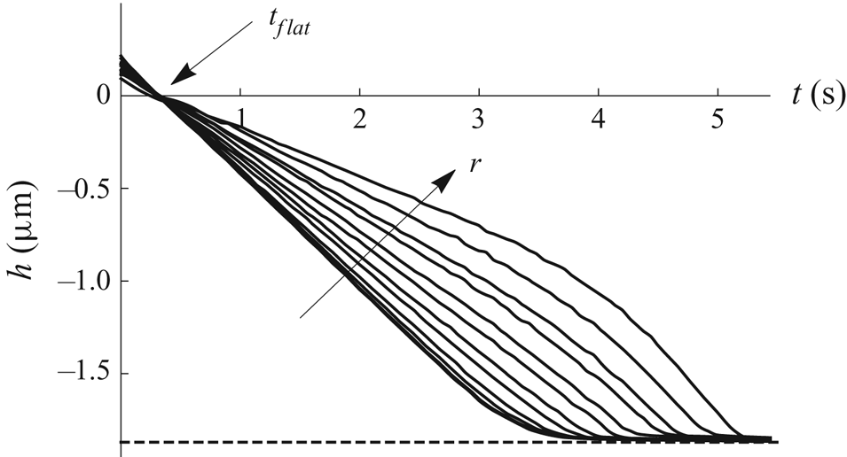
Figure 15. Experimental results for the free-surface profile  $h$ of a droplet as functions of
  $t$ for
  $r=0$, 4.29, 8.57, 12.86, 17.68, 20.90, 26.79, 30.01, 32.15, 34.83 and 38.04 for the
  $50$
$50$  $\mathrm {\mu }$m well. The arrow indicates the direction of increasing
  $r$. The dashed line corresponds to the depth
  $H_0=1.87$
  $\mathrm {\mu }$m of the well.
Figure 16 shows experimental results for the normalised height of the free surface at the centre of the well,  $h_{m}/H_0$, and linear fits to these values as functions of
  $t$ for all three wells. For each well, the time at which the free surface touches down at the centre of the well,
  $t_{touchdown}$, was calculated from the intersection point of the linear fit shown in figure 16 with the bottom of the well. However, note that whereas for the
  $29$
$29$  $\mathrm {\mu }$m well the behaviour of
  $h_{m}$ is nearly linear until very close to touchdown, and hence the value of
  $t_{touchdown}$ calculated from the linear fit will be very close to the true value, for the
  $50$
$50$  $\mathrm {\mu }$m and
  $75$
$75$  $\mathrm {\mu }$m wells the behaviour of
  $h_{m}$ shows a pronounced slowing down as touchdown is approached, and so the values of
  $t_{touchdown}$ calculated from the linear fits will be underestimates of the true values.
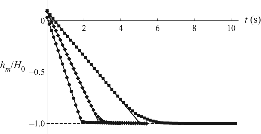
Figure 16. Experimental results for the normalised height of the free surface at the centre of the well,  $h_{m}/H_0$, (symbols) and linear fits to these values (solid black lines) as functions of
  $t$ for wells of radius
  $29$
$29$  $\mathrm {\mu }$m at times
  $t=0,0.12, \ldots , 3.96$ s,
  $50$
$50$  $\mathrm {\mu }$m at times
  $t=0,0.12, \ldots , 5.40$ s and
  $75$
$75$  $\mathrm {\mu }$m at times
  $t=0,0.16, \ldots , 10.24$ s. The experimental values are denoted by circles, diamonds and squares for the
  $29$
$29$  $\mathrm {\mu }$m,
  $50$
$50$  $\mathrm {\mu }$m and
  $75$
$75$  $\mathrm {\mu }$m wells, respectively. The dashed line corresponds to the normalised depth of the wells.
After touchdown, the interference fringes become increasingly closely spaced, making it increasingly difficult to resolve the free-surface profile near to the lip of the well. The resulting lack of experimental results for the free surface means that we cannot accurately determine it for very long after touchdown, and, in particular, that we cannot be certain that the contact line remains pinned at the lip of the well after touchdown (as assumed in the mathematical model). However, given the good agreement between the experimental results and the theoretical predictions of the mathematical model which will be described in § 7, we hypothesise that the effect of any de-pinning that does occur is minimal.
Figure 17 shows experimental results for the normalised volume of a droplet,  $V/V_0$, obtained by calculating the volumes of the paraboloidal fits to the free-surface profiles, and linear fits to these values as functions of
  $t$ for all three wells. Note that the difficulty of resolving the free-surface profile near to the lip of the well after touchdown means that the experimental values shown in figure 17 stop shortly after
  $t=t_{touchdown}$ for each well. However, figure 17 does show that the behaviour of
  $V$ is nearly linear until shortly after touchdown.
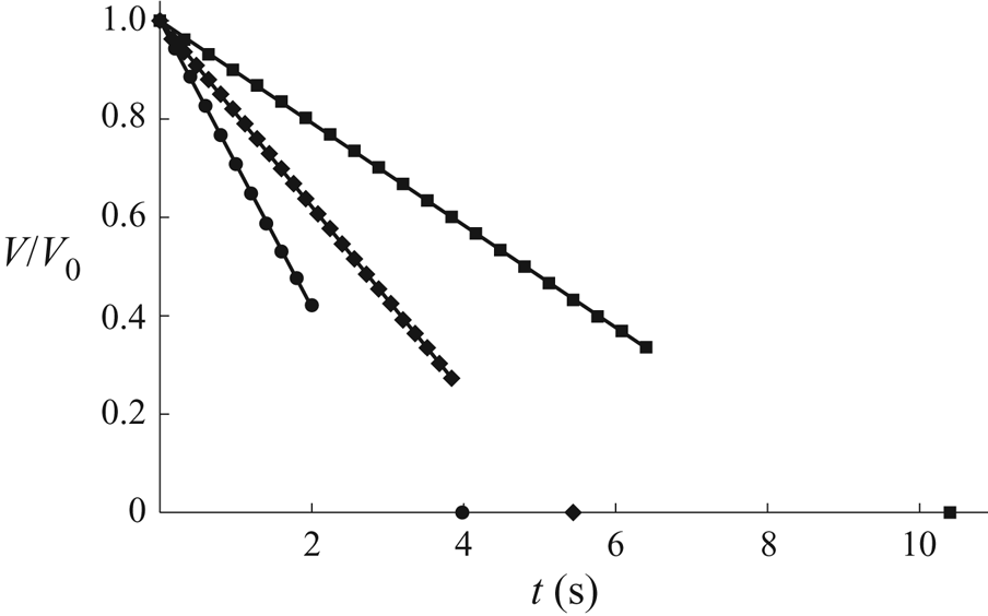
Figure 17. Experimental results for the normalised volume of a droplet,  $V/V_0$, (symbols) and linear fits to these values (solid black lines) as functions of
  $t$ for wells of radius
  $29$
$29$  $\mathrm {\mu }$m at times
  $t=0, 0.20, \ldots , 2.00$ s,
  $50$
$50$  $\mathrm {\mu }$m at times
  $t=0, 0.16, \ldots , 3.84$ s and
  $75$
$75$  $\mathrm {\mu }$m at times
  $t=0, 0.32, \ldots , 6.40$ s. The experimental values are denoted by circles, diamonds and squares for the
  $29$
$29$  $\mathrm {\mu }$m,
  $50$
$50$  $\mathrm {\mu }$m and
  $75$
$75$  $\mathrm {\mu }$m wells, respectively. The symbols on the
  $t$-axis correspond to
  $t=t_{lifetime}$.
Despite the interference fringes becoming increasingly closely spaced after touchdown, we were still able to measure accurately the radius of the inner contact line. This was accomplished by applying an appropriate threshold value to the intensity of the images of the droplets captured during the experiments. However, it should be noted that when the slope of the free surface is very small, this method is sensitive to the value of the threshold used and tends to overestimate the true value of  $R$. As previously noted, further details of the image-analysis procedure used are given in Appendix B. The receding inner contact line was occasionally observed to pin temporarily on a defect in the bottom of the well, but this distorted the contact line only in the immediate vicinity of the defect, and only for a time that was short compared with the time scale for the evaporation of the droplet. Figure 18 shows experimental values for the normalised radius of the inner contact line of a droplet,
  $R/R_0$, as functions of
  $t$ for all three wells.
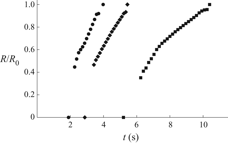
Figure 18. Experimental results for the normalised radius of the inner contact line,  $R/R_0$, as functions of
  $t$ for wells of radius
  $29$
$29$  $\mathrm {\mu }$m at times
  $t=2.32, 2.38, \ldots , 3.76$ s,
  $50$
$50$  $\mathrm {\mu }$m at times
  $t=3.38, 3.46, \ldots , 5.30$ s and
  $75$
$75$  $\mathrm {\mu }$m at times
  $t=6.24, 6.40, \ldots , 10.24$ s. The experimental values are denoted by circles, diamonds and squares for the
  $29$
$29$  $\mathrm {\mu }$m,
  $50$
$50$  $\mathrm {\mu }$m and
  $75$
$75$  $\mathrm {\mu }$m wells, respectively. The symbols on the
  $t$-axis correspond to
  $t=t_{touchdown}$, and those at
  $R/R_0=1$ to
  $t=t_{lifetime}$.
The lifetime of the droplet,  $t_{lifetime}$, was determined visually from the images of the droplet captured during the experiments as the time at which no further change is observed in the contrast at the contact line. The uncertainty in the measurement of
  $t_{lifetime}$ is
  $\pm 0.02$ s.
7. Comparison between theory and experiment
We now present comparisons between the theoretical predictions of the mathematical model described in §§ 2–4 in the case of a cylindrical well (i.e. in the limit  $n\to \infty$) and the experimental results presented in § 6. Specifically, we compare the evolution of the free-surface profile
  $h$, the volume of the droplet
  $V$ and the radius of the inner contact line
  $R$, as well as the critical times
  $t_{flat}$,
  $t_{touchdown}$ and
  $t_{lifetime}$. The theoretical predictions were calculated using the parameter values
  $\rho =1.087\times 10^{3}$ kg m
 $^{-3}$,
  $c_{sat}=2.251\times 10^{-3}$ kg m
 $^{-3}$ and
  $D=6.899\times 10^{-6}$ m
 $^{2}$ s
 $^{-1}$ for methyl benzoate at the temperature
  $22\,^{\circ }$C. The values of
  $\rho$ and vapour pressure
  $p_{v}$, the latter of which was used to obtain
  $c_{sat}$, were calculated from Perry, Green & Maloney (Reference Perry, Green and Maloney1997) (tables 2-30 and 2-6, respectively), and the value of the diffusion coefficient
  $D$ was calculated from Fuller, Schettler & Giddings (Reference Fuller, Schettler and Giddings1966) (table 1). Note that there are no free parameters in the mathematical model, and no ‘tuning’ of the parameter values has been performed in order to improve the agreement between the experimental results and the theoretical predictions.
As described in § 2, the mathematical model is based on the assumptions that both the Bond number  ${Bo}$ and the capillary number
  ${Ca}$ are small (so that the effect of gravity is negligible and the free surface of the droplet evolves quasi-statically, respectively). Taking the radial velocity scale to be
  $U=D(c_{sat}-c_{\infty })/(\rho \theta _0R_0)$, and using the values
  $\mu =1.851\times 10^{-3}$ Pa s and
  $\gamma =3.720\times 10^{-2}$ N m
 $^{-1}$ for methyl benzoate at
  $25\,^{\circ }$C given by Sheu & Tu (Reference Sheu and Tu2005), confirms that the values of
  ${Bo}$ and
  ${Ca}$ are indeed small for all of the experimental results presented in § 6. Specifically, the values of
  ${Bo}$ are approximately
  $10^{-4}$,
  $10^{-3}$ and
  $10^{-3}$ for the
  $29$
$29$  $\mathrm {\mu }$m,
  $50$
$50$  $\mathrm {\mu }$m and
  $75$
$75$  $\mathrm {\mu }$m wells, respectively, and the values of
  ${Ca}$ are approximately
  $10^{-2}$ for all three wells.
Figure 19 shows a comparison between the experimental results and the theoretical predictions for the free-surface profile  $h$ of a droplet as functions of
  $r$ for all three wells, while figures 20 and 21 show comparisons between the experimental results and the theoretical predictions for the normalised volume of a droplet,
  $V/V_0$, and the normalised radius of the inner contact line,
  $R/R_0$, respectively, as functions of
  $t$ for all three wells. In particular, figures 19–21 show that, while the theoretical predictions are generally in good agreement with the experimental results (especially for the
  $50$
$50$  $\mathrm {\mu }$m well), the theoretical predictions lag slightly behind the experimental results for the
  $29$
$29$  $\mathrm {\mu }$m and
  $75$
$75$  $\mathrm {\mu }$m wells. This slight lag is due to the sensitivity of the theoretical predictions to the precise values of
  $c_{sat}$ and
  $D$ used, as well as to the calculated values of
  $\theta _0$. In particular, as already mentioned, the ambient temperature was controlled only to within
  $1\,^{\circ }$C and the value of c sat is rather sensitive to the precise value of the temperature at which it is evaluated; specifically,
  $c_{sat}$ changes by
  $6$–
$6$– $8\,\%$ for a
  $1\,^{\circ }$C change in temperature. Fitting the value(s) of
  $c_{sat}$,
  $D$ and/or
  $\theta _0$ would eliminate the lag between the theoretical predictions and the experimental results, especially given that the same values of
  $c_{sat}$ and
  $D$ are currently used across all of the experiments, but we deliberately chose not to do this in order to provide a sterner test for the mathematical model.
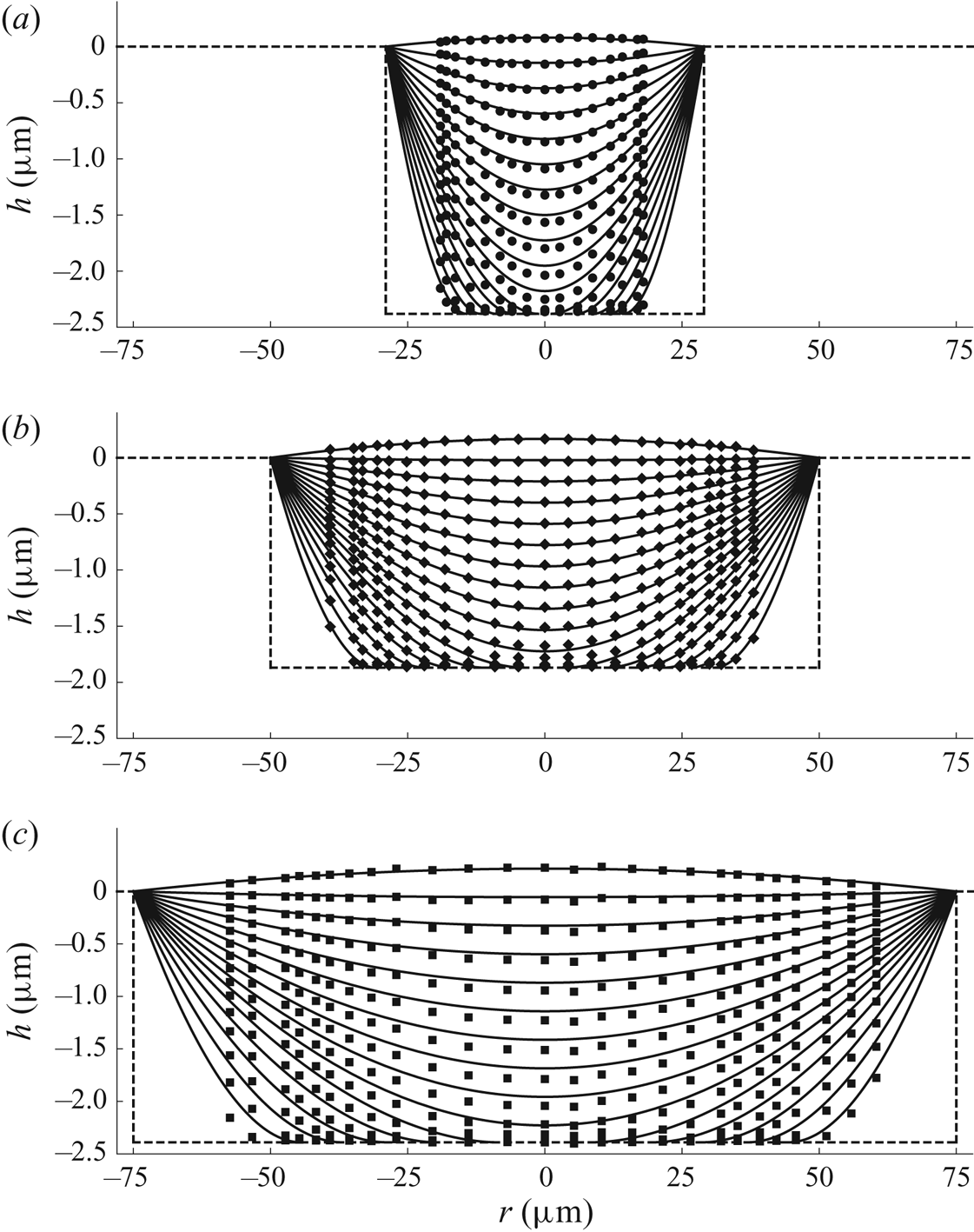
Figure 19. Comparison between the experimental results (symbols) and the theoretical predictions (solid black lines) for the free-surface profile  $h$ of a droplet as functions of
  $r$ for wells of radius (a)
  $29$
$29$  $\mathrm {\mu }$m at times
  $t=0, 0.18, \ldots , 2.70$ s, (b)
  $50$
$50$  $\mathrm {\mu }$m at times
  $t=0, 0.26, \ldots , 4.16$ s and (c)
  $75$
$75$  $\mathrm {\mu }$m at times
  $t=0, 0.56, \ldots , 7.84$ s. The experimental values are denoted by circles, diamonds and squares for the
  $29$
$29$  $\mathrm {\mu }$m,
  $50$
$50$  $\mathrm {\mu }$m and
  $75$
$75$  $\mathrm {\mu }$m wells, respectively. The dashed lines correspond to the radius
  $R_0$, the depth
  $H_0$, and the position of the dry substrate for each well.
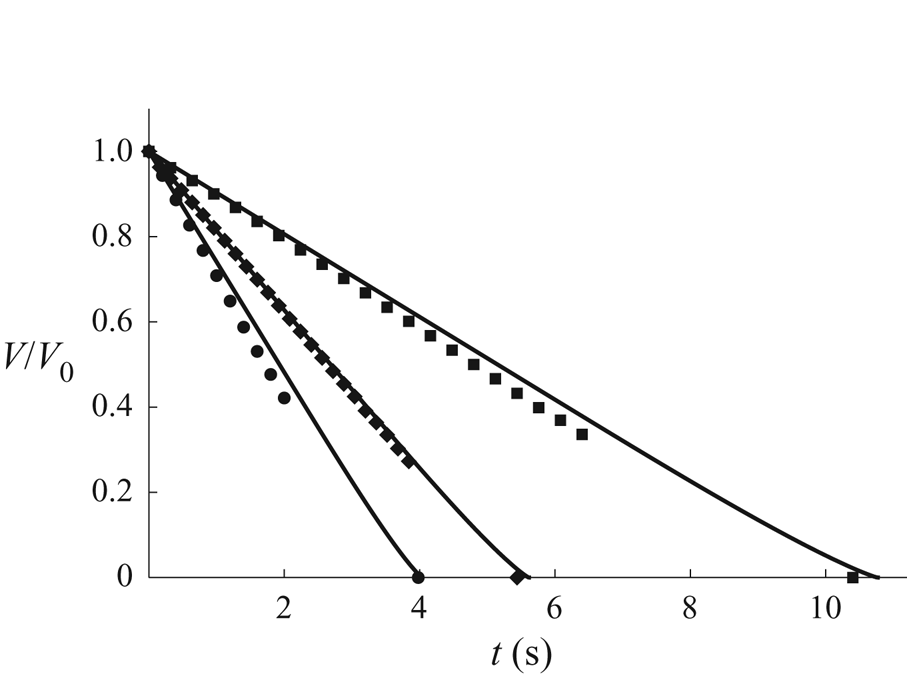
Figure 20. Comparison between the experimental results (symbols) shown in figure 17 and the theoretical predictions (solid black lines) for the normalised volume of a droplet,  $V/V_0$, as functions of
  $t$ for all three wells. The experimental values are denoted by circles, diamonds and squares for the
  $29$
$29$  $\mathrm {\mu }$m,
  $50$
$50$  $\mathrm {\mu }$m and
  $75$
$75$  $\mathrm {\mu }$m wells, respectively.
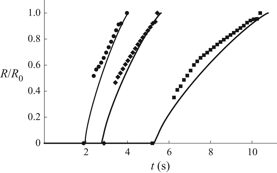
Figure 21. Comparison between the experimental results (symbols) shown in figure 18 and the theoretical predictions (solid black lines) for the normalised radius of the inner contact line,  $R/R_0$, as functions of
  $t$ for all three wells. The experimental values are denoted by circles, diamonds and squares for the
  $29$
$29$  $\mathrm {\mu }$m,
  $50$
$50$  $\mathrm {\mu }$m and
  $75$
$75$  $\mathrm {\mu }$m wells, respectively.
In addition, note that the mathematical model assumes that a new inner contact line appears at the centre of the well at touchdown, and so does not capture the very thin film left briefly on the bottom of the well in the experiments, which is most visible in the experimental results for the  $75$
$75$  $\mathrm {\mu }$m well shown in figure 19(c). However, the good agreement between the theoretical predictions and the experimental results shown in figures 19–21 indicates that the presence of this film has very little effect on the overall evolution of the droplet. At first sight, it might seem surprising that the most noticeable deviations from the quasi-static free-surface profiles predicted by the mathematical model occur for the shallowest well (i.e. for the well with the smallest value of
  $\epsilon$). However, while, as already mentioned, the values of
  ${Ca}$ are small for all three wells, the capillary number is inversely proportional to
  $\epsilon ^{3}$, and so larger values of
  ${Ca}$, and hence more significant deviations from quasi-static free-surface profiles, are to be expected for wells with smaller values of
  $\epsilon$.
As previously noted in § 6, the experimental values of the critical times depend on the arbitrarily chosen initial time,  $t=0$, as well as on the values of the ambient temperature and the atmospheric pressure. Moreover, as also previously noted, the theoretical predictions for the critical times are sensitive to the precise values of
  $c_{sat}$,
  $D$ and
  $\theta _0$. In order to remove all of these dependencies, we consider a parameter-free quantity involving the relative values of the critical times, namely
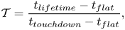 \begin{equation} {\mathcal{T}} = \frac{t_{lifetime}-t_{flat}}{t_{touchdown}-t_{flat}}, \end{equation}
which, using the theoretical values of the critical times given by (3.22), (3.24a) and (4.32), takes the same (purely numerical) value, namely  ${\mathcal {T}} = 1+8\alpha _{\infty } \simeq 2.095$, regardless of the values of the parameters. Table 2 shows a comparison between the experimental values and the theoretical predictions for
  $t_{flat}$,
  $t_{touchdown}$,
  $t_{lifetime}$ and
  ${\mathcal {T}}$ for all three wells. Table 2 shows that the theoretical predictions are in good agreement with the experimental values, with average absolute errors of approximately
  $9\,\%$,
  $3.8\,\%$,
  $2.8\,\%$ and
  $3.3\,\%$ in
  ${t_{flat}}$,
  ${t_{touchdown}}$,
  ${t_{lifetime}}$ and
  ${{\mathcal {T}}}$, respectively.
Table 2. Comparison between the experimental values and the theoretical predictions for the critical times  $t_{flat}$,
  $t_{touchdown}$ and
  $t_{lifetime}$, and the parameter-free quantity
  ${\mathcal {T}}$ given by (7.1) for all three wells.
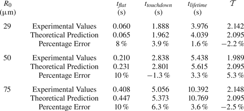
The comparisons presented in this section show that, despite the inevitable experimental errors and uncertainties about the precise values of the parameters, the mathematical model captures the evolution of a thin droplet in a shallow cylindrical well rather well. The agreement is especially good given that, as already mentioned, there are no free parameters in the mathematical model, and no tuning of the parameter values has been performed in order to improve the agreement.
8. Comparison with previous experimental results
While the experimental results presented in § 6 provide the most comprehensive test for the theoretical predictions of the mathematical model, it is also of interest to consider how well the present model is able to capture experimental results reported by previous authors. Making these comparisons is, unfortunately, hampered by a lack of complete information about the experiments.
Rieger et al. (Reference Rieger, van den Doel and van Vliet2003) studied the evaporation of ethylene glycol droplets in cylindrical nanolitre wells of various radii. In particular, they reported the evolution of the free-surface profile of a droplet before touchdown in a well with radius  $100$
$100$  $\mathrm {\mu }$m and depth
  $6.13$
  $\mathrm {\mu }$m, and concluded that it was a quasi-static spherical cap that was pinned at the lip of the well. Rieger et al. (Reference Rieger, van den Doel and van Vliet2003) gave the experimental values
  $t_{flat}=20$ s and
  $t_{touchdown}=160$ s, but not the experimental value of
  $t_{lifetime}$, for this droplet, and so, unfortunately, we cannot calculate the experimental value of the parameter-free quantity
  ${\mathcal {T}}$ given by (7.1). The authors also did not give the value of the initial angle
  $\theta _0$, but if we calculate it in essentially the same way as we did in § 6, we obtain
  $\theta _0=0.0144$. The value of the ambient temperature was also not reported, but if we assume that it was
  $20\,^{\circ }$C, then using the parameter values
  $\rho =1.114\times 10^{3}$ kg m
 $^{-3}$,
  $c_{sat}=2.042\times 10^{-4}$ kg m
 $^{-3}$ and
  $D=1.098\times 10^{-5}$ m
 $^{2}$ s
 $^{-1}$ calculated from Perry et al. (Reference Perry, Green and Maloney1997) (tables 2-30 and 2-6, respectively) and Fuller et al. (Reference Fuller, Schettler and Giddings1966) (table 1) in exactly the same way as we did in § 7, the theoretical predictions are
  $t_{flat}=14.05$ s and
  $t_{touchdown}=133.7$ s, which are in error by
  $30\,\%$ and
  $16\,\%$, respectively, compared with the experimental values. It should, however, be noted that, in addition to the uncertainties about the precise values of
  $c_{sat}$ and
  $D$ already mentioned, some of this discrepancy may be due to the fact that ethylene glycol is hygroscopic, and so the droplet will absorb water vapour from the atmosphere, which will presumably lead to longer critical times than those predicted by the present mathematical model. Rieger et al. (Reference Rieger, van den Doel and van Vliet2003) did not investigate the evolution of the droplet after touchdown.
Subsequently, Chen et al. (Reference Chen, Tseng and Chieng2006) studied the evaporation of water droplets in cylindrical nanolitre wells of various radii. The experiments were carried out in an atmosphere of air with relative humidity of water vapour of  $RH=0.60$ and an ambient temperature of
  $25\,^{\circ }$C. Chen et al. (Reference Chen, Tseng and Chieng2006) reported quantitative data for the evolution of the radius of the inner contact line
  $R$, but not for the evolution of the free-surface profile
  $h$ or the volume of the droplet
  $V$. Furthermore, they did not report the values of the initial angle
  $\theta _0$. They did, however, give the critical times for a droplet in a well with radius
  $250$
$250$  $\mathrm {\mu }$m and depth
  $65$
$65$  $\mathrm {\mu }$m to be
  $t_{flat} = 9 \pm 1$ s (estimated from their figure 9),
  $t_{touchdown} = 31$ s and
  $t_{lifetime} = 55$ s. In the absence of the value of
  $\theta _0$, the only theoretical prediction that can be compared with these experimental results is that for
  ${\mathcal {T}}$ for the well with radius
  $250$
$250$  $\mathrm {\mu }$m, for which we find that the experimental value
  ${\mathcal {T}}=2.09 \pm 0.05$ is in very good agreement with the theoretical value
  ${\mathcal {T}} \simeq 2.095$.
9. Conclusions
Motivated by the industrial manufacture of OLED displays, in the present work we formulated and analysed a mathematical model for the evolution of a thin droplet in a shallow axisymmetric well with profile  $z = H(r) = - H_0(1 - (r/R_0)^{n})$ both before and after touchdown that accounts for the spatially non-uniform evaporation of the fluid, performed physical experiments using three cylindrical wells with different small aspect ratios, and validated the mathematical model by comparing the present experimental results with the corresponding theoretical predictions for a cylindrical well (i.e. in the limit
  $n \to \infty$).
The mathematical model describes how as the droplet evaporates its free surface becomes instantaneously flat at  $t=t_{flat}$ and then touches down at
  $t=t_{touchdown}$ before the droplet completely evaporates at
  $t=t_{lifetime}$. In the special case
  $n = 2$ (i.e. a paraboloidal well) touchdown occurs everywhere simultaneously within the well, and so
  $t_{lifetime} = t_{touchdown} = {\rm \pi}(1+2H_0)/16$. However, in the general case
  $n \ne 2$ the droplet has not completely evaporated at
  $t = t_{touchdown}$, and the nature of its subsequent evolution depends on the shape of the well. If the slope of the well at its lip is sufficiently small, specifically when
  $0 < n < 2$, then touchdown occurs at the lip of the well at
  $t=t_{touchdown}$ given by (3.23a), at which instant the contact line de-pins from the lip of the well, and thereafter recedes towards the centre of the well, finally reaching it at
  $t=t_{lifetime}$ given by (4.16). On the other hand, if the slope of the well at its lip is sufficiently large, specifically when
  $n > 2$, then touchdown occurs at the centre of the well at
  $t=t_{touchdown}$ given by (3.24a), at which instant a new inner contact line appears at the centre of the well, and thereafter recedes towards the lip of the well (where the outer contact line remains pinned), finally reaching it at
  $t=t_{lifetime}$ given by (4.28). In particular, we found that
  $t_{flat}$ is independent of
  $H_0$ and
  $n$,
$n$,  $t_{touchdown}$ increases linearly with
  $H_0$ and with
  $n$ for
  $0 \le n \le 2$ but is independent of
  $n$ for
  $n > 2$, and
  $t_{lifetime}$ also increases linearly with
  $H_0$ but nonlinearly with
  $n$.
$n$.
The physical experiments involved depositing single droplets of methyl benzoate in three cylindrical wells with different small aspect ratios. Thin-film interferometry was used to determine the subsequent evolution of the free-surface profile of the fluid in the well. We found good agreement between the experimental results and the corresponding theoretical predictions for a cylindrical well. While the present mathematical model does not capture the very thin film left briefly on the bottom of the well in the experiments, the good agreement between the theoretical predictions and the experimental results indicates that the presence of this film has very little effect on the overall evolution of the droplet.
It should, of course, be emphasised that all of the experiments reported in the present work were in the parameter regime described by the mathematical model, namely thin droplets in shallow wells (i.e.  $\epsilon = H_0/R_0 \sim \theta _0 \ll 1$) with negligible gravity (i.e.
  ${Bo} \ll 1$) and strong surface tension (i.e.
  ${Ca} \ll 1$). Experiments outwith this regime can be expected to reveal additional behaviours not captured by the present model. For example, larger droplets with
  ${Bo} = O(1)$ will no longer have spatially constant mean curvature, while, as we have already mentioned, the free-surface profiles of thinner droplets and/or droplets of more volatile fluids with
  ${Ca} = O(1)$ will no longer evolve quasi-statically, and capturing such behaviours will require generalisations of the present model. Nevertheless, the results of the present work suggest that the present model is an excellent starting point for future work of this nature. Other interesting extensions of the present work include evaporation from wells with more complicated axisymmetric or non-axisymmetric profiles, other modes of evaporation, the final deposit left in the well after a droplet containing suspended particles has completely evaporated, and the interactions between droplets in neighbouring wells, with the latter two issues particularly relevant to the industrial manufacture of OLED displays. Moreover, in industrial applications a variety of additional physical effects which do not play a significant role in the present experiments, and hence are not included in the present mathematical model, may be important. For example, in situations in which significant evaporative cooling occurs, temperature-dependent surface tension (see, for example, Hu & Larson Reference Hu and Larson2005; Ristenpart et al. Reference Ristenpart, Kim, Domingues, Wan and Stone2007) and/or temperature-dependent saturation concentration (see, for example, Dunn et al. Reference Dunn, Wilson, Duffy, David and Sefiane2009; Sefiane et al. Reference Sefiane, Wilson, David, Dunn and Duffy2009; Schofield et al. Reference Schofield, Pritchard, Wilson and Sefiane2021) effects can be important, while in other situations buoyancy effects within the droplet (see, for example, Edwards et al. Reference Edwards, Atkinson, Cheung, Liang, Fairhurst and Ouali2018 and Li et al. Reference Li, Diddens, Lv, Wijshoff, Versluis and Lohse2019) and/or within the atmosphere (see, for example, Shahidzadeh-Bonn et al. Reference Shahidzadeh-Bonn, Rafaï, Azouni and Bonn2006; Dunn et al. Reference Dunn, Wilson, Duffy, David and Sefiane2009) may play an important role.
Acknowledgements
The authors wish to thank Professor A. Hazel (University of Manchester) for bringing several very helpful references to their attention.
Funding
H.-M.D'A. acknowledges financial support from the United Kingdom Engineering and Physical Sciences Research Council (EPSRC) via EPSRC Doctoral Training Partnership grant EP/R512205/1 and Merck Chemicals Ltd. T.C. acknowledges financial support from the National Productivity Investment Fund and Merck Chemicals Ltd.
Declaration of interests
The authors report no conflict of interest.
Appendix A. Fabrication of the wells
The wells used in the present experiments were fabricated in the Department of Engineering at Durham University. Polished glass ( $50\times 50\times 1.1$ mm) coated with ITO (
 $50$ nm thickness) was used as the substrate. The ITO-coated glass was cleaned in an ultrasound bath, using, in sequence, acetone, isopropyl alcohol (IPA) and deionised water. It was then dried with a nitrogen stream and warmed on a hot plate for 5 min. A negative photo-resist, SU-8 2002, was spin coated onto the substrate in two steps: a pre-spin at 500 r.p.m. for 10 seconds to spread and cover the entire surface of the ITO-coated glass, followed by a spin at 3000 r.p.m. for 1 min. After a soft-bake step at
  $95\,^{\circ }$C for 1 min on a hot plate, the substrate was exposed in hard-contact mode to UV light at
  $140\,\textrm {mJ}\,\textrm {cm}^{-2}$ using a photomask (Micro Lithography Services Ltd) which was designed according to the desired final pattern on the substrate. A post-exposure bake at
  $95\,^{\circ }$C for 1 min was used to cross-link the exposed film selectively. Then the SU-8 was developed with an ethylene carbonate developer solvent in a 1 min immersion process. Finally, the substrate was rinsed in IPA and dried with a nitrogen stream. Some samples were subjected to a hard bake at
  $200\,^{\circ }$C for 10 min to seal cracks in the patterned surface.
Appendix B. Image-analysis procedure
Interference microscopy images were processed using a MATLAB (The Mathworks Inc.) code that was developed in-house to obtain the free-surface profile of the droplet during evaporation (Kazmierski Reference Kazmierski2018). Interference between the reflected light from the fluid–air and fluid–solid interfaces is observed when the height of the film is less than the coherence length of the light source. The bright and the dark fringes shown in figure 13 represent constructive and destructive interference, respectively. Two neighbouring bright or dark fringes correspond to a height difference of  $\lambda /(2k) \simeq 155$ nm, where
  $\lambda$ is the wavelength of the light in a vacuum and
  $k$ is the refractive index of the fluid.
In view of the axisymmetry of the well and the droplet, it was sufficient to analyse the fringes along a cross-section through the centre of the well (as indicated by the line in figure 13). In order to avoid problems caused by closely spaced fringes near to the lip of the well which occur towards the end of the evaporation, we began by calculating the free-surface profile at a time  $t < t_{flat}$ at which the interference fringes were co-axial and the profile decreased monotonically in the radial direction. The evolution of the height of the free surface at the centre of the well,
  $h_{m}$, was determined by tracking the video frame-by-frame backwards in time from
  $t=t_{lifetime}$ (at which the height of the film is assumed to be zero) to the chosen initial frame. The initial free-surface profile was then calculated from the maxima and minima in the intensity along the cross-section of the image. The fringes near to the centre of the droplet were typically quite far apart, and so an additional 4 to 6 points on the profile were obtained by the backward-time-tracing method using a sinusoidal interpolation. A forward-time-tracing method was then used to track the frames forward in time, determining the free-surface profile of the droplet for the remainder of the evaporation in the same way as we calculated the initial profile. After touchdown, we set an appropriate threshold value of the intensity of the images and fitted a circle to the region of the image with intensity below this value in order to determine the radius of the receding inner contact line.


 Open access