


1. Introduction
In our environment where many flows are turbulent in nature, particles such as ice or debris in the air, or alternatively sediment, plankton or pollutants in the ocean, can interact with multiple scales of turbulent eddies as well as bounding surfaces. These complicated particle/turbulence and particle/wall interactions can affect how particles are transported in the environment or separately in industrial processes related to the transport of pharmaceuticals, recyclables or waste, wherein a given particle can either lift off from, collide with, or slide, roll or saltate along bounding surfaces.
Research investigating particle-laden flow is challenging due to the complexity in modelling or reconstructing both fluid and particle motions across a wide range of length scales (Eaton & Fessler Reference Eaton and Fessler1994). In many previous numerical simulations of wall-bounded flows, to simplify the problem, particles were modelled as point-masses with no volume and thus no rotation (e.g. Pedinotti, Mariotti & Banerjee Reference Pedinotti, Mariotti and Banerjee1992; Dorgan & Loth Reference Dorgan and Loth2004; Soldati & Marchioli Reference Soldati and Marchioli2009; Mortimer, Njobuenwu & Fairweather Reference Mortimer, Njobuenwu and Fairweather2019). However, as noted in the recent review by Brandt & Coletti (Reference Brandt and Coletti2022), particle size can be important in addition to particle inertia. For flows with non-negligible particle Reynolds number ( $Re_p = |\boldsymbol {U}_{rel}|d/\nu$, where $\boldsymbol {U}_{rel}$ is the slip velocity vector between the fluid and the particle, $d$ is the particle diameter, and $\nu$ is the fluid kinematic viscosity), the particle response time alone is insufficient to quantify either particle motions or particle/turbulence interactions. The study by Costa, Brandt & Picano (Reference Costa, Brandt and Picano2020) comparing the results between interface-resolved and one-way-coupled point-particle direct numerical simulations (DNS) revealed that the point-mass model failed to model the particle velocity accurately due to the absence of shear-induced lift force (see also Apte, Mahesh & Lundgren Reference Apte, Mahesh and Lundgren2008; Lee & Balachandar Reference Lee and Balachandar2010). In this context, the particle size can determine how its motions are affected by eddies of varying size and strength, how particles affect velocity variations within the boundary layer due to, for example, vortex shedding (van Hout et al. Reference van Hout, Eisma, Elsinga and Westerweel2018), and how discrete particles interact with bounding surfaces. Until recently, particle-resolved simulations in wall-bounded flows have been relatively limited due to their high computational cost and related challenges in achieving fine-scale resolution (Apte et al. Reference Apte, Mahesh and Lundgren2008; Balachandar & Eaton Reference Balachandar and Eaton2010; Horne & Mahesh Reference Horne and Mahesh2019; Subramaniam Reference Subramaniam2020).
Considering experiments, early studies by Sutherland (Reference Sutherland1967), Francis (Reference Francis1973), Abbott & Francis (Reference Abbott and Francis1977) and Drake et al. (Reference Drake, Shreve, Dietrich, Whiting and Leopold1988), among others, examined the transport of individual grains above sediment or rough beds using traditional imaging techniques. More recent work incorporated velocity measurement techniques to investigate both the particle and fluid phases. Many of these studies focused on statistical velocity distributions of small inertial particles and their correlations with the streamwise–wall-normal turbulent Reynolds stresses (e.g. Séchet & Le Guennec Reference Séchet and Le Guennec1999; Kiger & Pan Reference Kiger and Pan2002; Nezu & Azuma Reference Nezu and Azuma2004; Righetti & Romano Reference Righetti and Romano2004; Lelouvetel et al. Reference Lelouvetel, Bigillon, Doppler, Vinkovic and Champagne2009; Zade et al. Reference Zade, Costa, Fornari, Lundell and Brandt2018; Ebrahimian, Sanders & Ghaemi Reference Ebrahimian, Sanders and Ghaemi2019; Zhu et al. Reference Zhu, Pan, Wang, Liang and Ji2019). Fundamental work focused on quantifying dynamics of individual neutrally or negatively buoyant particles based on the surrounding flow field is more limited. van Hout (Reference van Hout2013) combined time-resolved particle image velocimetry (PIV) and particle tracking velocimetry (PTV) to track individual small polystyrene beads (diameter  $d^+=10$) at friction Reynolds number $Re_{{\tau }}=435$. This study illustrated that particle lift-off from the wall was correlated with fluid ejections generated by passing vortex cores and corresponding increases in shear. The statistical analysis by Baker & Coletti (Reference Baker and Coletti2021) helped to quantify the role of ejections in lifting polystyrene particles away from the wall. Once lifted beyond the buffer layer, polystyrene particles either remained suspended in the fluid or saltated along the smooth wall, depending on the type and strength of coherent structures that they encountered. Ahmadi, Sanders & Ghaemi (Reference Ahmadi, Sanders and Ghaemi2021), who plotted multiple pathlines of suspended glass beads, reported that particles in the outer region of the boundary layer ascend, descend or undergo multiple upwards and downwards motions, similar to those observed by Sumer & Oğuz (Reference Sumer and Oğuz1978) and Tee, Barros & Longmire (Reference Tee, Barros and Longmire2020). Except for Tee et al. (Reference Tee, Barros and Longmire2020), both particle Reynolds number and Stokes number, defined based on the ratio of particle response time to a characteristic flow time, were typically small in previous studies such that vortex shedding was either absent or assumed to be negligible. Recently, van Hout et al. (Reference van Hout, Hershkovitz, Elsinga and Westerweel2022), who performed time-resolved tomographic PIV on freely moving, nearly neutrally buoyant spheres ( $d^+ \sim 70$) in a turbulent boundary layer ( $Re_\tau =390$), reported that in four tracked runs, the instantaneous $Re_p$ were mostly less than 100, and no vortex shedding was observed.
Aside from its wall-normal motion, a particle can also migrate in the spanwise direction due to turbulent fluid motions. Many previous studies noted the preferential accumulation of smaller particles within long slow-moving streamwise structures or streaks near the wall (e.g. Rashidi, Hetsroni & Banerjee Reference Rashidi, Hetsroni and Banerjee1990; Pedinotti et al. Reference Pedinotti, Mariotti and Banerjee1992; Kaftori, Hetsroni & Banerjee Reference Kaftori, Hetsroni and Banerjee1995a,Reference Kaftori, Hetsroni and Banerjeeb; Marchioli & Soldati Reference Marchioli and Soldati2002; Picciotto, Marchioli & Soldati Reference Picciotto, Marchioli and Soldati2005; Sardina et al. Reference Sardina, Schlatter, Brandt, Picano and Casciola2012; Berk & Coletti Reference Berk and Coletti2020; Wang & Richter Reference Wang and Richter2020). The spanwise motion of larger particles both close to and further from the wall remains poorly understood, however. Kaftori et al. (Reference Kaftori, Hetsroni and Banerjee1995a) and Niño & García (Reference Niño and García1996) noted that particles with diameters larger than the viscous sublayer thickness had a lesser tendency to accumulate in long low-speed streaks. In this context, the study by Ahmadi, Sanders & Ghaemi (Reference Ahmadi, Sanders and Ghaemi2020) on polystyrene beads of  $d^+=26$ reported that the conditionally averaged particle spanwise velocity was stronger than the particle wall-normal velocity as well as the surrounding spanwise fluid velocity, hypothetically due to the beads preserving their spanwise velocities for longer durations than the fluid phase. In our previous work (Tee et al. Reference Tee, Barros and Longmire2020), spanwise velocities of lifting spheres also exceeded the corresponding wall-normal velocities.
The work mentioned thus far considered the effects of mean shear, turbulence and the bounding surface on particle motions. Apart from these factors, Magnus lift (Magnus Reference Magnus1853) induced by the rotation of a particle moving relative to a fluid can also play a role. Both frictional torque induced at a wall and hydrodynamic torque generated by local velocity gradients can induce sphere rotation (e.g. Saffman Reference Saffman1965; Cherukat, McLaughlin & Dandy Reference Cherukat, McLaughlin and Dandy1999; Bagchi & Balachandar Reference Bagchi and Balachandar2002; Bluemink et al. Reference Bluemink, Lohse, Prosperetti and van Wijngaarden2008; Lee, Ha & Balachandar Reference Lee, Ha and Balachandar2011). Here, the lift coefficient from flow past a transversely rotating sphere depends on both  $Re_p$ and the dimensionless rotation rate $\alpha =\varOmega d/2U_{rel}$ where $\varOmega$ is the sphere angular velocity (Poon et al. Reference Poon, Ooi, Giacobello, Iaccarino and Chung2014). Among others, White & Schulz (Reference White and Schulz1977) and Niño & García (Reference Niño and García1994), who compared experimental and theoretical reconstructed particle saltation trajectories in turbulent boundary layer flows, concluded that Magnus lift could be a non-negligible part of the overall particle lift force. However, as in the other experiments mentioned above, these authors did not quantify particle rotation explicitly. Several numerical studies in turbulent wall-bounded flows, including those of Zhao & Andersson (Reference Zhao and Andersson2011), Ardekani & Brandt (Reference Ardekani and Brandt2019), Peng, Ayala & Wang (Reference Peng, Ayala and Wang2019) and Esteghamatian & Zaki (Reference Esteghamatian and Zaki2021), reported that particle rotation can not only affect particle transport but also induce significant effects on the fluid turbulence.
Our earlier experiments (Tee et al. Reference Tee, Barros and Longmire2020), which focused on both translation and rotation of relatively large individual spheres (initial  $Re_p = 760$ and $1840$) in a turbulent boundary layer, demonstrated several interesting effects. First, Magnus lift was important for a relatively dense particle (specific gravity $\rho _p/\rho _f=1.152$, and $d^+=56$), enabling it to lift off from the underlying wall. After it was released from rest, this sphere initially slid along the wall before eventually starting to roll forwards. It lifted off the wall only after the sphere began to rotate continuously with a dimensionless rotation rate of 0.6 and 0.4 when $Re_\tau =680$ and 1320, respectively. Meanwhile, spheres close to neutrally buoyant typically lifted off from the wall immediately, and mostly translated above it with minimal rotation. All three spheres tested tended to lag the local mean unperturbed velocity of the fluid, and their instantaneous velocity varied up to $20\,\%$ from the local mean value. Particle Reynolds numbers, defined based on the relative streamwise velocity using the mean unperturbed velocity profile, suggested values ranging from 100 to 500. Therefore, based on the simulations of Zeng et al. (Reference Zeng, Balachandar, Fischer and Najjar2008), where vortex shedding was always present for $Re_p>200$, the experimental spheres, especially the denser ones, were frequently also in a shedding regime. Finally, all spheres were observed to translate significantly in the spanwise direction, up to 12 % of the streamwise distance travelled.
Given the particle behaviours observed in Tee et al. (Reference Tee, Barros and Longmire2020), the objective of the work described herein was to track both finite spheres (with initial  $Re_p=730$ and $1730$) and the surrounding fluid motions over relatively long distances to further investigate the physics behind the fluid/particle interactions. For example, since the spheres travelled within the logarithmic region, interactions with the dominant large-scale structures there, i.e. long coherent slow- and fast-moving regions (Ganapathisubramani, Longmire & Marusic Reference Ganapathisubramani, Longmire and Marusic2003; Tan & Longmire Reference Tan and Longmire2017), likely influence the particle velocity variations observed. Similar to Tee et al. (Reference Tee, Barros and Longmire2020), individual particles were released from rest and tracked using three-dimensional (3-D) PTV over a long streamwise distance. Surrounding fluid motions were investigated simultaneously using stereoscopic PIV (SPIV) in streamwise–spanwise planes at multiple streamwise and wall-normal locations to resolve fluid length scale down to $0.4d$. Multiple sphere densities and friction Reynolds numbers were considered to study the effects of specific gravity and mean shear on sphere motions. It is our goal that these experimental data can serve as a benchmark for testing and improving predictive models for particle transport in various flow applications. The paper is organized as follows. Section 2 describes the facility, methods, experimental parameters and measurement uncertainty; § 3 presents results on sphere motion, and how sphere velocity, forward rotation, lift-offs, descents and spanwise motions are affected by the surrounding fluid motion. The conclusions are summarized in § 4.
2. Methodology
In this paper,  $x$,
$x$,  $y$ and $z$ define the streamwise, wall-normal and spanwise directions, respectively. Instantaneous fluid velocity components in the $x$,
$x$,  $y$ and $z$ directions are represented by $U$,
$U$,  $V$ and $W$, with lowercase letters ( $u'$,
$u'$,  $v'$ and $w'$) indicating fluctuating components after subtraction of ensemble average values denoted by an overline ( $\bar {U}$, $\bar {V}$ and $\bar {W}$). Subscript ‘ $o$’ denotes quantities measured in the unperturbed fluid, while subscripts $f$ and $p$ denote quantities represented by the fluid and particle, respectively. Superscript $+$ denotes quantities normalized by the inner scaling, namely friction velocity ( $u_\tau$) and $\nu$.
2.1. Facility
All experiments were conducted in a recirculating water channel facility at the University of Minnesota. The flow is driven by a Reliance Electric AC motor coupled with three propellers in parallel pipes located beneath the test section. After passing through a set of perforated plates followed by turning vanes, the flow is straightened and conditioned with a honeycomb section and three screens before being accelerated through a contraction of ratio  $5\,:\,1$ ahead of the test section. The glass test section is 8 m long, 1.12 m wide and 0.61 m deep. For all experiments, a 3 mm cylindrical trip wire located at the test section entrance triggered the development of a turbulent boundary layer along the bottom wall. The free stream turbulence intensity is 1 % (Saikrishnan Reference Saikrishnan2010). A coarse grid was positioned at the downstream end of the test section to enable recapture of the spheres used in the experiments. A thorough description of the facility can be found in Gao (Reference Gao2011).
2.2. Sphere fabrication
To achieve a repeatable and controllable initial condition, magnetic spheres of diameter  $d=6.35\,{\rm mm}$ were fabricated in-house from a mixture of blue machinable wax ( $913.7\,{\rm kg}\,{\rm m}^{-3}$) and synthetic black iron oxide particles ( $5170\,{\rm kg}\,{\rm m}^{-3}$) using two hemisphere molds made from aluminium. The resulting spheres were black and opaque. A step-by-step illustration of the fabrication procedure is depicted in Tee (Reference Tee2021).
Sphere density was controlled by varying the amount of iron oxide added to the melted wax. The actual density ( $\rho _p$) of each sphere was determined from high-speed image sequences of the sphere falling through quiescent fluid obtained with a Phantom M110 camera at sampling frequency 200 Hz. Once the sphere was travelling at its settling velocity ( $V_s$), its density was calculated using $\rho _p = 3C_D\rho _fV_s^2/4dg + \rho _f$, where the drag coefficient ( $C_D$) as a function of sphere settling Reynolds number ( $V_sd/\nu$) was obtained from the standard drag curve in Clift, Grace & Weber (Reference Clift, Grace and Weber1978). Here, $g$ is the gravitational acceleration.
Based on the sphere translation and rotation reconstruction methodology proposed by Barros, Hiltbrand & Longmire (Reference Barros, Hiltbrand and Longmire2018), small markers were painted manually at arbitrary locations all over the sphere surface using a white oil-based pen for tracking purposes (see the inset in figure 1b). Both the mean inter-marker spacing and mean marker diameter were approximately 0.6 mm.

Figure 1. Schematic of experimental set-up (not to scale). (a) Top view: two pairs of high-speed cameras (T1 and T2) with infrared-block filters, aligned in stereoscopic configurations for capturing the trajectory and rotation of a marked sphere over a long field of view. (b) Cross-section view: one pair of stereoscopic high-speed cameras (C1a and C1b) with infrared-pass filters, positioned under the channel to capture fluid motion in the streamwise–spanwise plane illuminated by the infrared laser. The sphere was held in place by a magnet attached to a solenoid. Inset: sphere captured in greyscale, with  $d$ spanning ${\sim }43$ pxs.
2.3. Characterization of turbulent boundary layers
Velocity statistics of the unperturbed turbulent boundary layers were determined from planar PIV measurements in streamwise–wall-normal planes at the initial particle release location 4.2 m downstream of the trip wire. The flow was seeded with silver-coated hollow glass spheres from Potters Industries LLC with average diameter and density  $13\,\mathrm {\mu }{\rm m}$ and $1600\,{\rm kg}\,{\rm m}^{-3}$, respectively. A New Wave Solo II Nd $:$YAG 532 nm double-pulsed laser system was used for illumination. The laser sheet illuminated through the bottom glass wall had thickness 1 mm. Measurements were conducted at two motor frequencies, 20 and 45 Hz. At each flow condition, sets of 2400 image pairs were acquired at sampling frequency 1.12 Hz using a TSI Powerview Plus 4MP 16-bit CCD camera with $2048 \times 2048$ pixels (pxs). The camera pixel size was $7.4\,\mathrm {\mu }{\rm m}$, and the magnification was 0.061 mm per pixel.
Raw PIV images were processed using DaVis 10 (LaVision GmbH). First, a background subtraction was performed to remove the strong light reflection near the bottom wall. Then a PIV cross-correlation with Gaussian filtering was implemented using an overlap of 50 % over initial interrogation window sizes of  $48 \times 48$ pxs followed by three passes of $24 \times 24$ pxs. The universal outlier detection criterion (Westerweel & Scarano Reference Westerweel and Scarano2005) was applied to remove spurious vectors. The spatial resolution of the resulting velocity vectors (based on 24 pxs window size) was 1.46 mm, or approximately 13 and 27 viscous units when $Re_\tau =670$ and 1300, respectively.
Mean velocity profiles were obtained by averaging the vectors across the 2400 image pairs and across the streamwise range imaged. The friction velocity was estimated by employing the Clauser chart method with log-law constants  $B=5$ and von Kármán constant $\kappa =0.41$ (Clauser Reference Clauser1956; Monty et al. Reference Monty, Hutchins, Ng, Marusic and Chong2009). Then the friction Reynolds numbers ( $Re_\tau = u_\tau \delta /\nu$) were computed using boundary layer thicknesses estimated based on the location where the mean unperturbed streamwise fluid velocity reached $99\,\%$ of the free stream value or $\overline {U_o(\delta )}=0.99 U_\infty$. The momentum thickness Reynolds numbers $Re_{{\theta _m}}=U_\infty \theta _m/\nu$ were computed based on the momentum thickness
 \begin{equation} \theta_m= \int_{0}^{\infty} \frac{\overline{U_o(y)}}{U_\infty}\left(1-\frac{\overline{U_o(y)}}{U_\infty}\right){{\rm d} y}. \end{equation}
The boundary layer properties are summarized in table 1.
Table 1. Summary of turbulent boundary layer properties.

2.4. Sphere-tracking measurements
Two of the same spheres from Tee et al. (Reference Tee, Barros and Longmire2020) (P1 and P3) with density ratios ( $\rho _p/\rho _f$) 1.006 and 1.152 were investigated due to their contrasting lifting and wall-interacting motions. The same 3-D PTV set-up was employed. For each run, a sphere was held statically on the smooth glass wall in the boundary layer by a cubic N40 magnet located 4.2 m downstream of the trip wire, and 0.3 m (approximately $4\delta$) away from the nearest sidewall based on the sphere centroid (figure 1b). This location will be considered as the origin in $x$ and $z$, with the bottom wall as $y=0$. A DC 12 V 2 A push–pull type solenoid from Uxcell held the cubic magnet under the channel. When the power supply was switched on (solenoid ON), the solenoid and a plunger/slider mechanism held the magnet flush with the outer channel wall. To release the sphere, the power supply was switched off so that the plunger and magnet would retract with the help of gravity. When the magnet moved away from the bottom wall, the sphere was allowed to propagate with the incoming flow.
Two pairs of Phantom v210 high-speed cameras from Vision Research ( $1280 \times 800\,{\rm pxs}$) were arranged in stereoscopic configurations looking through the sidewall to track the sphere motion over streamwise distance $5\delta$ (figure 1a). The angle between the two stereoscopic cameras was set to approximately $30^\circ$ for both camera pairs, as suggested by Barros et al. (Reference Barros, Hiltbrand and Longmire2018), to maximize the number of common markers observed. The camera pairs were positioned with a streamwise overlap in a field of view of approximately two particle diameters. All cameras were fitted with Scheimpflug mounts and Nikon Micro-Nikkor 105 mm lenses with aperture $f/16$. The far outer sidewall of the water channel was covered with white plastic to increase the contrast between the black-marked sphere and the imaging background. Two white LED panels positioned above the cameras illuminated the domain considered. The camera pixel size was $20\,\mathrm {\mu }{\rm m}$, and the magnification was 0.15 mm per px. This corresponded to an imaged sphere diameter of approximately 43 pxs in both camera pairs.
Prior to running the experiments, the 3-D PTV optical system was calibrated by displacing a two-level plate (LaVision Type 22) across up to five planes surrounding the initial spanwise position of the sphere. Separate calibrations were performed for each sphere-tracking camera pair. Then a third-order polynomial fit for each calibration plane was used to generate the mapping function of the volumetric calibration via the classic stereoscopic calibration routine of DaVis. The images from all sphere-tracking cameras were first pre-processed using a MATLAB standard circular Hough transform routine (figure 2a) to isolate the sphere from the background (figure 2b). The extracted sphere images from both camera pairs were then imported separately to DaVis 10. Here, the images were further processed with  $3 \times 3$ Gaussian smoothing (figure 2c), sharpening filters (figure 2d), and intensity thresholding (see figure 2e) to isolate the dots from the sphere image for tracking purposes. In all images, the minimum digital dot size was approximately $2 \times 2\,{\rm pxs}$. Subsequently, a 3-D PTV routine based on the respective volumetric calibration mapping function was implemented to reconstruct the dot coordinates from each camera pair.

Figure 2. Sphere image pre-processing to isolate the dots on the sphere surface for 3-D PTV. (a) Original image superposed with a circle identified using a MATLAB circular Hough transform routine. (b) Image with background removed. (c) Gaussian filtered image. (d) Sharpening filtered image. (e) Final image after intensity thresholding.
The data sets obtained from DaVis included the 3-D coordinates of true and ghost markers, and their corresponding velocity vectors. The ghost markers were generated due to ambiguity in reconstruction of images from only two cameras. Since the true markers must lie on the sphere surface, the filtering methodology proposed by Barros et al. (Reference Barros, Hiltbrand and Longmire2018) was employed to remove the ghost tracks. The sphere centroid was determined by fitting the true marker coordinates to the equation of a sphere. Then a rotation matrix that best aligned the markers of consecutive images was obtained by applying the Kabsch (Reference Kabsch1976) algorithm. At least 8 markers were retained when computing the sphere centroid locations and rotation matrices.
2.5. Simultaneous fluid velocity measurements
Time-resolved SPIV measurements were conducted simultaneously with the 3-D PTV to obtain the three components of fluid velocity surrounding the tracked sphere within an  $x$–
$x$– $z$ plane at a fixed height (see figure 1). Here, an Oxford Firefly high-frequency infrared pulsed laser with wavelength 808 nm and coupled sheet optics were positioned between the two pairs of sphere-tracking cameras to illuminate tracer particles. A third pair of high-speed cameras (Phantom M110, $1280\times 800\,{\rm pxs}$) viewed through the bottom channel wall to capture the fluid motion (see figure 1b). These cameras were fitted with Scheimpflug mounts and Nikon Micro-Nikkor 60 mm lenses with aperture $f/2.8$. The angle between each camera and the wall-normal axis was approximately $25^\circ$. For optimal imaging of the tracer particles, infrared-pass filters were added to the SPIV cameras. Infrared-block filters were added to the sphere-tracking cameras. The SPIV camera magnification was 0.085 mm per px.
As the SPIV camera frame was obstructed by the sphere release mechanism, fluid measurement fields were captured starting at  $x\sim 0.2\delta$. The SPIV measurements had a field of view of approximately $1.4\delta \times 0.9\delta$. Experiments for each sphere at both $Re_\tau$ were repeated at multiple streamwise and wall-normal positions. These locations were selected based on the results in Tee et al. (Reference Tee, Barros and Longmire2020) in order to understand the role of the fluid in causing sphere lift-offs, eventual descents after reaching a peak, spanwise motions, and the transition from sliding to forward rotation that contributed to the small repeated lift-off events observed for sphere P3. As the sphere could be lifted entirely out of the fluid measurement plane, we will focus on fluid results where the sphere intersects the laser sheet. Due to the streamwise velocity variations at different laser sheet heights and $Re_\tau$, the sampling frequency, which also corresponded to the pulse separation ( $\Delta t$) for time-resolved fluid and sphere motion measurements, was varied between 240 Hz and 540 Hz, depending on the case, so that tracer particle displacements fell within the one-quarter rule (Adrian & Westerweel Reference Adrian and Westerweel2011).
For SPIV calibration, a two-level plate (LaVision Type 22) was placed parallel to the bottom wall at a height matching the laser sheet position. Then a third-order polynomial fit was obtained using the classic stereoscopic calibration routine in DaVis to generate a mapping function. Next, stereoscopic self-calibration using 200 image pairs was carried out on top of the classic calibration up to four times until the results converged. In the raw SPIV images, the large and opaque sphere obstructed the laser light illuminating from the sidewall obscuring the tracer particles in that region. The moving sphere also appeared as a very bright spot. Thus the SPIV images were pre-processed in MATLAB to replace the sphere image with image intensity value 0 to minimize its effect on fluid cross-correlations. The resulting images were then processed using DaVis 10. The spatial auto-mask function was implemented to mask out the sphere and its shadow. To enhance velocity vector reconstruction, sliding sum-of-correlation with a filter length of 2 time steps was implemented (see Sciacchitano, Scarano & Wieneke Reference Sciacchitano, Scarano and Wieneke2012). An overlap of 50 % over initial interrogation window sizes of  $64 \times 64\,{\rm pxs}$ followed by three passes of $32 \times 32\,{\rm pxs}$ was employed to obtain the three-component velocity vectors. Gaussian weighting was applied to all windows, and spurious vectors were removed based on the universal outlier detection criterion (Westerweel & Scarano Reference Westerweel and Scarano2005). The spatial resolutions of the computed SPIV velocity vectors (for a window of 32 pxs) were 24 and 50 viscous units at $Re_{{\tau }}$ of 670 and 1300, equivalent to 2.73 mm.
To estimate the local fluid velocity at the sphere position ( $\boldsymbol {U}_f$), we averaged the fluid velocity vectors in a region of 1.4 $d$ length $\times$ 2.8 $d$ span centred on the upstream half of the sphere. Downstream vectors were ignored to avoid the velocity deficit in the sphere wake. We tested multiple region sizes, and found that the $\boldsymbol {U}_f$ estimates did not vary significantly when the region was changed by $\pm 0.4d$ in either dimension. With the chosen region (shown below in figure 8), about 60 fluid vectors were averaged for each estimate.
2.6. Summary of experimental parameters
The experimental parameters for the cases run are summarized in table 2. Spheres P1 and P3 ( $d=6.35\pm 0.05$ mm) with $\rho _p/\rho _f=1.006$ and 1.152, respectively, were considered at two flow speeds corresponding to $Re_\tau =670$ and 1300, $d^+= 56$ and 116 viscous units, $d/\delta =0.084$ and 0.089, and $d/\eta = 25$ and 44, respectively where $\eta$ refers to the Kolmogorov length scale at the height of the particle diameter (Pope Reference Pope2000). The initial $Re_p=|\boldsymbol {U}_{rel}|\,d/\nu$ values, based on mean $|\boldsymbol {U}_{rel}| = 0.114$ and $0.271\,{\rm m}\,{\rm s}^{-1}$ at the particle centre upon release, were 730 and 1730. Note that although $|V_s|/U_\infty$ is relatively small for sphere P1, it is very significant for P3. Here, the particle Stokes numbers ( $St^+$, $St_\delta$) expressed as the ratio of particle response time $\tau _p=(2\rho _p+\rho _f)d^2/36\nu \rho _f$ (Crowe Reference Crowe2005) to the characteristic flow time scale based on the viscous time scale ( $t^+=\nu /u_\tau ^2$) and largest time scale ( $\delta /U_\infty$), range from 262 to 1230, and 9.1 to 23.5, respectively. Different representations of Stokes numbers using $\tau _{p,g}=\rho _pd^2/18\nu \rho _f$, which is commonly used in gas–solid flow to characterize the time required for a particle to reach the surrounding fluid velocity, as well as $\tau _{p,t}=(\rho _p-\rho _f)d^2/18\nu \rho _f$, which is defined based on the time required for a particle to reach terminal settling velocity in quiescent fluid, are compared to the $St^+$ defined above (see Brandt & Coletti Reference Brandt and Coletti2022). In other words, the ratios of $\tau _{p,g}$ and $\tau _{p,t}$ to $\tau _p$, which are equivalent to ${2\rho _p}/({2\rho _p+\rho _f})$ and ${2(\rho _p-\rho _f)}/({2\rho _p+\rho _f})$, are computed respectively.
Table 2. Summary of experimental parameters, where  $\overline {U_o(y={d}/{2})}$ represents the mean unperturbed fluid velocity at the initial sphere centroid position. Stokes numbers are $St^+=\tau _p/t^+$ and $St_\delta =\tau _p/(\delta /U_\infty )$, where $\tau _p=(2\rho _p+\rho _f)d^2/36\nu \rho _f$, $\tau _{p,g}=\rho _pd^2/18\nu \rho _f$, $\tau _{p,t}=(\rho _p-\rho _f)d^2/18\nu \rho _f$ and $t^+=\nu /u_\tau ^2$. Initial mean wall-normal force ratio $\overline {F_y}^*=(\overline {F_y}-F_b)/F_b$, where $\overline {F_y}$ denotes the mean wall-normal fluid-induced force based on the Hall (Reference Hall1988) expression, and $F_b=(\rho _p - \rho _f){\rm \pi} d^3g/6$ denotes the net buoyancy force.

The experiments were repeated at the laser sheet positions listed in table 3 to cover different portions of sphere trajectories. Since the spheres tended to move in the spanwise direction as they travelled downstream, the streamwise–spanwise measurement plane at position C was shifted towards  $+z$ to ensure that the particle remained within the SPIV field of view during approximately half of the runs. For each laser sheet position and case considered, up to 10 sphere trajectories and fluid flow sequences were captured and saved. However, only those results where part of the sphere intersected the laser sheet through more than $80\,\%$ of the field of view were included when computing statistics. The respective number of runs considered is thus listed in table 3 as $J$. Despite the shorter streamwise SPIV field of view, the sphere motions were reconstructed over trajectories of up to $5\delta$ for all runs for completeness.
Table 3. Summary of SPIV measurements, where  $x_{spiv}$, $y_{spiv}$ and $z_{spiv}$ represent the SPIV measurement domain in $x$,
$x$,  $y$ and $z$, respectively, $\overline {U_{o}(y_{spiv})}$ represents the mean unperturbed fluid velocity averaged over the SPIV measurement plane, and $J$ represents the number of runs considered for each case, with a subscript representing the sphere.

2.7. Measurement uncertainty
The uncertainty of 3-D PTV vectors is dominated by triangulation error. The root mean square (r.m.s.) error of the grid point positions from the calibration using a classical third-order polynomial fit was between 0.05 px and 0.1 px, indicating an optimal fit. The mean disparity error for individual marker position ( $\epsilon _{disp}^*$), calculated by projecting the 3-D reconstructed markers back to the camera image in DaVis, was approximately 0.8 px. This gives an uncertainty estimate in the individual marker locations due to triangulation errors (Wieneke Reference Wieneke2008).
To reduce the noise in computing derivatives, the raw sphere position and orientation data were smoothed by a quintic spline (Epps, Truscott & Techet Reference Epps, Truscott and Techet2010). The uncertainties of sphere position ( $x$,
$x$,  $y$,
$y$,  $z$) and orientation ( $\theta _x$, $\theta _y$, $\theta _z$) were computed based on the r.m.s. of the difference between the raw and smoothed data, as suggested by Schneiders & Sciacchitano (Reference Schneiders and Sciacchitano2017). The mean uncertainties were then obtained by averaging the r.m.s. values over all runs. For sphere position, the mean values were 0.40, 0.30 and 0.77 px; for orientation, the values were 0.72, 0.76 and 0.30 px, respectively. In terms of translational and angular displacement, these correspond to 0.9 %, 0.7 % and 1.9 % of the sphere diameter, and $1.9^\circ$, $2.2^\circ$ and $0.8^\circ$, respectively. Finally, the mean uncertainties of the translational sphere velocities ( $U_p$, $V_p$, $W_p$) were estimated to be 2 %, 1 % and 4 % of $U_\infty$.
For the SPIV calibration, the standard deviations of the classical third-order polynomial plane fit were in the range 0.05–0.2 px for all SPIV conditions. After self-calibration, the standard deviation was less than 0.001 px. The reconstruction errors computed in DaVis based on the deviation of the reconstructed velocity vectors ( $U, V, W$) from the velocity vectors obtained via planar computation ( $(U_{C{1{a}}}, W_{C{1{a}}})$ for camera C1a, and $(U_{C{1{b}}}, W_{C{1{b}}})$ for camera C1b) were all below 0.5 px, indicating optimal reconstruction (Wieneke Reference Wieneke2005).
The SPIV velocity vectors are also affected by the uncertainty in peak-finding of the instantaneous velocity vectors from each camera (Adrian & Westerweel Reference Adrian and Westerweel2011). As the apparent streamwise and spanwise velocity vectors of the first camera are triangulated with those of the second camera to obtain the three-component velocity vectors, the uncertainties of SPIV vectors can be calculated through error propagation of each of the apparent velocity vectors ( $\delta _{U_{C{1{a}},C{1{b}}}}$), which is a function of the angle between the line of sight of the camera and the $z$-axis (Wieneke Reference Wieneke2005). For a symmetric angle $25^\circ$ and a peak-finding error for an instantaneous planar PIV vector $\delta _{U_{C{1{a}},C{1{b}}}}\approx 0.1\,{\rm px}$, this results in $\delta _U=0.08$, $\delta _V=0.17$ and $\delta _W=0.07\,{\rm px}$. At both $Re_\tau$ values, these values are equivalent to 1 %, 2 % and $0.9\,\%$ of $U_\infty$. The out-of-plane wall-normal velocity has the highest uncertainty, as expected.
Two-point velocity correlations between sphere and fluid velocities yielded relatively large uncertainties. Although the total number of measurements correlated across multiple runs and multiple time steps per run was large in all cases (e.g.  $N\approx 2000\unicode{x2013}4000$), the number of independent measurements was much smaller due to the persistence of large-scale fluid structures within a given run. Using estimates for the number of independent structures correlated, P1 at $Re_\tau =1300$ yielded the highest uncertainty ${\sim }0.1$ for streamwise correlations, while both P1 and P3 at $Re_\tau =670$ yielded the lowest values, ${\sim }0.04\unicode{x2013}0.07$. Due to the larger uncertainty for $W_p$, uncertainties for spanwise correlations were larger ( ${\sim }0.2$) except for P3 at $Re_\tau =670$, which had uncertainty ${\sim }0.11$.
3. Results and discussion
3.1. Unladen turbulent boundary layer
The wall-normal profiles of the unperturbed turbulent boundary layers as listed in table 1 are plotted in figure 3. At both  $Re_\tau$ values, the profiles of the mean unperturbed streamwise velocity ( $\overline {U_o}$) match very well with the canonical turbulent boundary layer as simulated by Jiménez et al. (Reference Jiménez, Hoyas, Simens and Mizuno2010) at similar $Re_\tau$. Small deviations near the wall are likely due to insufficient spatial resolution. The mean velocities of the SPIV measurements at three locations at both $Re_\tau$ values as listed in table 3 are superposed on the profiles as filled symbols. These values were also used to verify the exact heights of the laser sheet, which were challenging to estimate precisely as the infrared laser is invisible to human eyes. The unperturbed wall-normal profiles of the streamwise turbulent intensities ( $u^+_{o,rms}$), computed based on Reynolds decomposition, also show good agreement with the simulation (see figure 3b). The $u^+_{o,rms}$ values for the SPIV measurements are also superposed as filled symbols. Here, the magnitudes in the wall-parallel measurements are generally smaller than those measured in the wall-normal PIV, likely due to the coarser interrogation windows used (see also Saikrishnan, Marusic & Longmire Reference Saikrishnan, Marusic and Longmire2006). The canonical mean boundary layer profiles at both $Re_\tau$ values are also plotted in figure 3(c) in physical height normalized by the sphere diameter. It is clear that the spheres investigated in this study span the strongest wall-normal shearing zone near the wall.

Figure 3. Wall-normal profiles of the unperturbed turbulent boundary layers at  $Re_\tau =670$ (blue) and 1300 (red): (a) mean streamwise fluid velocity and (b) r.m.s. of the streamwise fluctuating velocity in wall units, and (c) mean streamwise fluid velocity superposed with a 6.35 mm sphere plotted in black for scale reference. Empty symbols indicate wall-normal planar PIV data. Filled symbols indicate wall-parallel SPIV data as noted in table 3. Lines in (a,b) indicate DNS profiles from Jiménez et al. (Reference Jiménez, Hoyas, Simens and Mizuno2010).
3.2. Overview of sphere motion
Figure 4 shows wall-normal trajectories reconstructed from the current study for spheres P1 (black) and P3 (purple) at  $Re_\tau =670$ and 1300, while figure 5 depicts the sphere orientation about the spanwise axis and sphere spanwise positions at $Re_\tau =670$. All cases considered in the current study exhibited sphere behaviours similar to those reported in Tee et al. (Reference Tee, Barros and Longmire2020).

Figure 4. Spheres P1 (black) and P3 (purple) wall-normal trajectories plotted based on centroid location at (a)  $Re_\tau =670$ and (b) $Re_\tau =1300$. Darker and lighter solid lines correspond with measurements at laser sheet positions A and B or C, respectively, as marked by red and pink shaded regions (see table 3). Black markers in (a) represent different runs of P1 as depicted in figures 6(a), 7 and 9(a). Here, the light grey shaded region with dark grey ‘ $\times$’ represents the extent of the sphere cross-section for one sample run marked by black ‘ $\times$’. Black markers ‘ $+$’ in (b) represent one sample run of P1 as plotted in figures 6(b), 9(b) and 16(b). Black markers ‘ $\circ$’ highlight one lift-off example at laser sheet position A.

Figure 5. Plots for  $Re_\tau =670$: (a) sphere orientation about spanwise axis, and (b) sphere spanwise position. Black indicates sphere P1, and purple indicates sphere P3. Darker and lighter lines correspond to SPIV measurements at laser sheet positions A and C, respectively, as marked by red and pink shaded regions in figure 4(a) (see also table 3). The inset in (a) shows a zoomed view of five P3 runs offset from one another on the vertical axis for clarity.

Figure 6. Sphere streamwise velocity  $U_p$ normalized by mean unperturbed streamwise fluid velocity at the local height of the sphere centroid ( $\overline {U_{o}(y_c)}$) at (a) $Re_\tau =670$ and (b) $Re_\tau =1300$. Black indicates sphere P1, and purple indicates sphere P3. Darker and lighter lines represent sphere data from laser sheet positions A and B or C, respectively (see table 3). Black markers in (a) represent specific runs depicted in figures 4(a), 7 and 9(a). Purple markers represent the runs depicted in figures 8 and 9(a). Black ‘ $+$’ markers in (b) represent the run depicted in figures 4(b), 9(b) and 16(b).

Figure 7. Time series contour plots of streamwise fluctuating velocity ( $u'$) surrounding sphere P1 at $Re_\tau =670$ for runs (a) ‘ $\circ$’ and (b) ‘ $\times$’ as marked in black in figures 4(a), 6(a) and 9(a), normalized by the unperturbed fluid velocity at laser sheet position A ( $y/d=0.7$). Black region indicates sphere. Grey region indicates sphere shadow. Black and green contours represent clockwise and anticlockwise swirling structures.

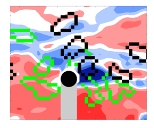
Figure 8. Time series contour plots of streamwise fluctuating velocity ( $u'$) surrounding sphere P3 at ${Re_\tau =670}$ for runs (a) purple ‘ $+$’, when $0.4< x/\delta <1.6$, and (b) purple ‘ $\square$’, when $1.4< x/\delta <2.6$, as marked in purple in figures 6(a) and 9(a), normalized by the unperturbed fluid velocity at laser sheet positions A and C ( $y/d=0.7$). Black region indicates sphere. Grey region indicates sphere shadow. Black and green contours represent clockwise and anticlockwise swirling structures. Purple boxes in (a) mark shed vortices. Brown box in the bottom plot of (b) outlines the region of fluid vectors used in estimating $U_f$ and is superposed with velocity vectors for reference.

Figure 9. Streamwise relative velocity ( $U_{rel}=U_f-U_p$) normalized by free stream velocity (left-hand axis) and friction velocity (right-hand axis) at (a) $Re_\tau =670$ and (b) $Re_\tau =1300$. Here, $U_f$ is local fluid velocity averaged over an area $1.4d \times 2.8d$ vector spaces upstream from the sphere centroid position. Black indicates sphere P1, and purple indicates sphere P3. Darker and lighter lines represent data from laser sheet positions A and B or C, respectively (see table 3). Black markers in (a) represent different runs in figures 4(a), 6(a), 7, 13, 15 and 16(a). Purple markers in (a) represent different runs in figures 6(a), 8, 11, 12 and 19. Black ‘ $+$’ markers in (b) represent the run depicted in figures 4(b), 6(b) and 16(b). For reference, $Re_d=U_\infty d/\nu =1300$ and 2950 in (a) and (b), respectively.
At both  $Re_\tau$ values, sphere P1 accelerated strongly and almost always lifted off the wall upon release. It always ascended to a peak height before descending towards the wall and ascending again with or without wall collision. Sphere P1 ascended to greater heights at larger $Re_\tau$ (figure 4b) due to stronger mean shear (Hall Reference Hall1988; Tee et al. Reference Tee, Barros and Longmire2020). Yousefi, Costa & Brandt (Reference Yousefi, Costa and Brandt2020) concluded also that the mean flow, irrespective of the initial turbulent structures, was responsible for initial particle lift-offs. While the initial lift-off is prompted by the strong mean shear due to large relative velocity ( $\overline {F_L}^* > 0$ in table 2), after the sphere accelerates and translates with the incoming fluid, the mean shear lift must decrease. As the lifting sphere P1 did not rotate much while translating (see Tee et al. Reference Tee, Barros and Longmire2020), the Magnus effect was insignificant. Hence the subsequent lift-offs, which could reach greater heights than the initial ones, must be aided by wall-normal forces related to the surrounding fluid motions.
The denser sphere P3 did not lift off upon release but translated along the wall at both  $Re_\tau$ values (purple in figure 4). The plots in figure 5(a) show that the sphere initially slid along the wall for approximately one boundary layer thickness before beginning to rotate forwards at a relatively constant rate. Repeated lift-off events with peak heights $\Delta y \leq 0.2d$ followed the onset of forward rotation. As reported in Tee et al. (Reference Tee, Barros and Longmire2020), these small lift-offs were aided by Magnus lift, which was more important at lower $Re_\tau$ because the sphere travelled with a higher dimensionless rotation rate. The small peak heights of sphere P3 demonstrate that the upward impulse associated with the Magnus lift is insufficient to oppose the net downward force after the sphere detaches from the wall. As in Tee et al. (Reference Tee, Barros and Longmire2020), all sphere/wall collisions were inelastic, thus the lift-offs were not due to wall rebound.
In all cases, the sphere migrated significantly in the spanwise direction (see figure 5b). Most of the larger spanwise motions occurred when the sphere was first released and relative velocities were highest. For P3 at  $Re_{{\tau }}=670$ and prior to forward rolling, the spanwise trajectories exhibited shorter wavelength fluctuations than in the other cases.
In the next few subsections, we will first look at how the sphere streamwise velocity is affected by the surrounding mean flow and turbulent structures. The corresponding laser sheet positions are marked in red in figure 4. Then, as sphere P3 at  $Re_\tau =670$ exhibited significant forward rotation, we will discuss the fluid results surrounding this sphere to understand the onset of this rotation, which is also important to the Magnus lift. We will then focus on fluid results related to sphere P1 ascents and descents. Finally, we will analyse the effects of fluid motions on spanwise sphere migration.
3.3. Sphere and fluid streamwise velocities
Figure 6 shows sphere velocity versus downstream distance for multiple runs of all four cases. These plots, which focus on streamwise locations included in the SPIV measurements, show sphere velocity normalized by the mean unperturbed fluid velocity at the local sphere height interpolated from figure 3 (i.e.  $\overline {U_{o}(y_c)}$). In all cases except that of sphere P3 at $Re_\tau =670$, the spheres accelerated strongly within $x/\delta \sim 0.2$ before reaching an approximate terminal velocity. Although sphere P3 initially travelled at approximately 30 % of the local mean fluid velocity, it began to accelerate again after $x/\delta \sim 1.5$. This acceleration, which is closely related to forward rolling motion as shown in figure 5, will be discussed in § 3.4. This sphere reaches an approximate terminal velocity $0.7\,\overline {U_{o}(y_c)}$ beyond $x/\delta = 2.8$.
In figure 6, the normalized sphere velocity varies by more than  $20\,\%$ across different runs in each case. In general, it also varies substantially within each run. For sphere P1, the variation within a run correlates somewhat with its wall-normal position, as highlighted in Tee et al. (Reference Tee, Barros and Longmire2020). However, the velocity variation across different runs does not correlate directly with wall-normal position. In some runs, the sphere also travels faster than the mean fluid velocity at the sphere centroid height, highlighting the importance of local turbulence structures. By contrast, even though sphere P3 did not lift off the wall early in its trajectory, its streamwise velocity varied significantly during a given run and between runs. Thus the wall-normal position is not the only reason behind the velocity variations.
In Tee et al. (Reference Tee, Barros and Longmire2020), we suggested that the variation in sphere streamwise velocity is likely due to long coherent structures that appear as alternating fast- and slow-moving zones, or high- and low-velocity regions (Dennis & Nickels Reference Dennis and Nickels2011b; Tan & Longmire Reference Tan and Longmire2017). To verify our hypothesis, we first look at time series of streamwise fluid velocity contours for two contrasting runs of sphere P1 at  $Re_\tau =670$ (see figure 7). These runs are marked in figures 4(a) and 6(a) for reference. Note that the fluctuating streamwise velocity ( $u'$) is computed by subtracting the mean unperturbed fluid velocity from the instantaneous velocity.
The signed two-dimensional swirling strength, plotted as black and green contours in figure 7 to represent clockwise and anticlockwise swirls, is computed from the imaginary part of the complex eigenvalue of the local velocity gradient tensor  $\lambda _{ci}(x,z)$, as $\varLambda _{ci}(x,z)\equiv \lambda _{ci}(x,z)\,({\omega _y(x,z)}/{|\omega _y(x,z)|})$ (see Zhou et al. Reference Zhou, Adrian, Balachandar and Kendall1999; Tomkins & Adrian Reference Tomkins and Adrian2003) and the sign of the instantaneous wall-normal vorticity $\omega _y(x,z)$. Then swirling regions including four or more grid points above a threshold $|\varLambda _{ci}(x,z)|>0.5\varLambda _{ci}^{rms}(x,z)$ are identified (see Wu & Christensen Reference Wu and Christensen2006).
In figure 7(a), sphere P1 travels across a field of view of  $1.2\delta$ while surrounded by a low-velocity region (blue contours). The region is bounded by pairs of clockwise and anticlockwise swirls that likely indicate legs of hairpin vortices that form a vortex packet as reported by Ganapathisubramani et al. (Reference Ganapathisubramani, Longmire and Marusic2003), Tomkins & Adrian (Reference Tomkins and Adrian2003) and Gao, Ortiz-Duenas & Longmire (Reference Gao, Ortiz-Duenas and Longmire2011). These structures can extend along multiple boundary layer thicknesses in the streamwise direction and typically span ${\sim }0.6\delta$ (Hutchins, Ganapathisubramani & Marusic Reference Hutchins, Ganapathisubramani and Marusic2005; Zheng & Longmire Reference Zheng and Longmire2014). The corresponding sphere velocity, marked by a black ‘ $\circ$’ in figure 6(a), is slower than in the other runs for this case. By contrast, the same sphere travelling in a high-velocity region (figure 7b) travels faster (black ‘ $\times$’ in figure 6a). This high-velocity region may be formed by forward induction from the series of neighbouring vortex legs in two adjacent hairpin packets (Tomkins & Adrian Reference Tomkins and Adrian2003). Thus we can infer from figure 6 that spheres moving at lower speeds are likely travelling in lower-velocity regions, and vice versa. Note that in other runs (not shown), this sphere encountered both low- and high-velocity regions, causing its velocity to vary over a wide range within the run. For example, a sphere travelling within a fast-moving zone may lag the fluid and eventually be overtaken by an approaching slow-moving zone. Similarly, a sphere travelling in a slow-moving zone can subsequently be accelerated by an approaching fast-moving zone. This scenario is observed more frequently with sphere P3, which will be considered next.
Sample flow sequences for sphere P3 at the lower  $Re_\tau$ over different streamwise ranges are plotted in figure 8. As this sphere translated unsteadily along the wall, it was overtaken repeatedly by both low- and high-velocity regions, as shown in figure 8(a). Distinct wake features are visible downstream of sphere P3 as indicated by the regions with strong $-u'$, and these wakes interact with the surrounding structures in the boundary layer. Vortex shedding can be identified from pairs of black and green contours downstream of the sphere and marked by the purple boxes in figure 8(a). The shed vortices appear as pairs of counter-rotating vortices, which could be slices of hairpin-like loops, as observed by van Hout et al. (Reference van Hout, Eisma, Elsinga and Westerweel2018) using tomographic PIV. Even though the shed vortices appear similar in the contour plots to the hairpin vortices found in the long coherent structures, the shed vortices marked in the boxes are stronger than the latter, with normalized $|\varLambda _{ci}(x,z)|$ values 1.5 times as high. The larger values for the shed vortices make sense because the large velocity deficit in the wake generates stronger streamwise velocity differences and circulation across a similar spanwise length scale. Even after this sphere has accelerated to a higher velocity downstream, shed vortices are still identifiable as depicted in figure 8(b), suggesting that the sphere still lags the surrounding fluid significantly. Both the velocity lag (combined with passing turbulent structures) and the intermittent vortex shedding can cause sphere P3's streamwise velocity to fluctuate more rapidly than that of sphere P1. Analysis based on Hutchins & Marusic (Reference Hutchins and Marusic2007) suggests that the largest amplitude variations in a given P3 run correspond with passage frequencies of alternating fast- and slow-moving flow structures. Frequencies associated with vortex shedding (discussed in more detail below) are 2–3 times higher.
To understand forcing effects on the sphere and to estimate when vortex shedding may be present, we compute the sphere relative velocity as  $\boldsymbol {U}_{rel}=\boldsymbol {U}_f - \boldsymbol {U}_p$, and the local particle Reynolds number $Re_p = |\boldsymbol {U}_{rel}|\, d/\nu = Re_d\,|\boldsymbol {U}_{rel}|/U_\infty$, where $Re_d=U_\infty d/\nu =1300$ and $2950$ for $Re_\tau =670$ and $1300$, respectively. The brown box upstream of the sphere in figure 8(b) shows the region of fluid used to estimate the fluid velocity components, as explained in § 2.5. Since $\boldsymbol {U}_p$ is obtained at the sphere centroid height, and $\boldsymbol {U}_f$ is obtained at the fixed height $y/d=0.7$, relative velocities will be estimated only for examples where the sphere partially intersected the laser sheet. Although the computed $U_{rel}$ may overestimate the true relative velocity for a sphere centred below the laser sheet, and vice versa, the trend over the trajectory typically depends more on the variations in fluid speed ( $u'/U_\infty \sim 14\,\%$) than on the variations in sphere wall-normal position. For sphere P1 at both $Re_\tau$ values, we estimate that the uncertainty in $U_{rel}$ due to varying sphere height is ${\pm }5\,\%$. For sphere P3, which typically travels along the wall, $U_{rel}$ may be overestimated by approximately 5 % and 4 % for $Re_\tau =670$ and $1300$, respectively.
Figure 9 shows  $U_{rel}$ for sphere trajectories in all four cases. At $Re_\tau =670$, the streamwise relative velocity is almost always positive for both spheres such that they lag the local flow structures. For example, sphere P1 travelling in the low-velocity region in figure 7(a) (marked by black ‘ $\circ$’ in figure 9a) still lags the fluid, travelling with instantaneous particle Reynolds number $Re_p\sim 250$. (In general, $U_{rel}$ dominates the other components in $\boldsymbol {U}_{rel}$ and in determining $Re_p$.) By contrast, sphere P1 travelling in the high-velocity region in figure 7(b) (marked by black ‘ $\times$’ in figure 9a) is accelerated more strongly by the high-velocity region and propagates at a streamwise velocity closer to the local fluid value. At $Re_\tau =1300$, $U_{rel}$ is negative in some runs for sphere P1, all corresponding with laser sheet position A. The corresponding fluid velocity fields (not shown) suggest that in some runs, due to its large inertia, the sphere retains higher streamwise momentum after it is surrounded by a lower velocity region. Also, in one run where the sphere centroid is above the laser sheet, $U_f$ may be underestimated, leading to a negative relative velocity. In another run, the sphere travels within a narrow, high-velocity region sandwiched between two low-velocity regions. Oversampling of the low-velocity fluid upstream of the sphere when estimating $U_f$ may have led to a negative relative velocity estimate. The runs corresponding with laser sheet position B all yield positive $U_{rel}$. In these examples, the sphere has risen further above the wall and likely had insufficient time to reach the local fluid velocity. For sphere P3, the streamwise relative velocity is always positive at both $Re_\tau$ values, and almost always larger than for sphere P1.
Fully resolved DNS by Zeng et al. (Reference Zeng, Balachandar, Fischer and Najjar2008) on a fixed sphere embedded in a turbulent boundary layer concluded that vortex shedding was occasionally present when  $Re_p>100$, and always present when $Re_p>200$. For sphere P3 at $Re_\tau =670$, $Re_p$ is estimated as 560 and 260 in the upstream and downstream portions of figure 9(a), suggesting that vortex shedding was omnipresent. At $Re_\tau =1300$, wherever $U_{rel}/U_\infty >0.1$ in figure 9(b), $Re_p > 295$, implying that vortex shedding was present most of the time. These results are consistent with our earlier observation in figure 8 of paired swirling structures in the sphere's wake. Examination of multiple runs indicated that streamwise spacing between neighbouring wake structures was $0.2\delta \unicode{x2013}0.35\delta$, with an associated range for the Strouhal number $Str = fd/|\boldsymbol {U}_{rel}|$ of $0.25\unicode{x2013}0.45$. These values are higher than the value identified by van Hout et al. (Reference van Hout, Eisma, Elsinga and Westerweel2018), where $Str$ was found to increase from 0.14 to 0.20 for a tethered sphere of $d^+=50$ at $Re_\tau =352$ as the gap between the sphere and underlying wall decreased from 301 to 18 viscous units ( $Re_p$ also decreased from 959 to 692). For a fixed sphere in uniform flow, $Str=0.18\unicode{x2013}0.21$ when $300 < Re_p < 800$ (Sakamoto & Haniu Reference Sakamoto and Haniu1990).
This behaviour can be contrasted with that of the lifting sphere P1. After P1 accelerates steeply from rest, its  $Re_p$ decreases from initial values near 730 and 1730 at $Re_\tau =670$ and $1300$ to a range $0< Re_p<300$. If we consider the run for this sphere marked by black ‘ $\times$’ in figure 9(a), then the instantaneous $Re_p \sim 100$ suggests the absence of any vortex shedding. A close look into the SPIV sequence associated with figure 7(b) confirmed this absence. Here, the region of slow-moving fluid downstream and in the $-z$ spanwise direction relative to the sphere is most likely the wake left behind after the sphere accelerated from rest (see figure 7b). van Hout et al. (Reference van Hout, Hershkovitz, Elsinga and Westerweel2022) did not observe vortex shedding among their four tracked runs with a sphere of $d^+ \sim 70$ at $Re_\tau =390$. Although the density of their spheres was similar to that of P1, over a streamwise distance of one boundary layer thickness, their spheres stayed within the range $40< y^+<160$ (based on centroid positions) with $Re_p<100$.
On the other hand, during the run where sphere P1 travelled more slowly than the fluid average (marked by black ‘ $\circ$’ in figure 9a), $Re_p \sim 250$, suggesting occasional vortex shedding. However, any wake vortices are most likely weaker than those observed for sphere P3, where $Re_p$ is larger. Thus they could not be differentiated distinctively from the surrounding turbulent hairpin structures. For the cases considered then, vortex shedding can play an important role not only in affecting the instantaneous drag on a sphere, but also in modifying the turbulence organization. This is especially true when the particle interacts with the wall and lags behind the fluid. When vortex shedding is present, it can also affect the instantaneous wall-normal force, as noted by Zeng et al. (Reference Zeng, Balachandar, Fischer and Najjar2008) and van Hout et al. (Reference van Hout, Eisma, Elsinga and Westerweel2018).
Considering the effect of vortex shedding on sphere motion, we noted that prior to rolling forwards continuously, sphere P3 oscillated forwards and backwards unsteadily, as shown in the inset of figure 5(a). As a given oscillation lasted more than 20 time steps, the fluctuations were not due to noise in processing. The power spectral density of the sphere orientation about the  $z$-axis for $0< x/\delta <2$ (not shown here) yields a peak matching the shedding $Str$ estimate given above. In Tee et al. (Reference Tee, Barros and Longmire2020), we reported that the sphere streamwise and spanwise velocities fluctuated at a lower $Str\sim 0.1\unicode{x2013}0.2$. We noted a similar range for $U_p$ and $W_p$ in the present work. As stated above, however, these lower frequency fluctuations are more likely correlated with oncoming fast- and slow-moving zones.
A statistical study by Baker & Coletti (Reference Baker and Coletti2021) with small polystyrene particles ( $d^+=16$ and $Re_\tau =570$) reported a mean relative velocity of order $u_\tau$. In the range $y^+>20$, particles lagged the fluid due to oversampling of fluid regions with negative streamwise fluctuations. A similar observation was reported by Berk & Coletti (Reference Berk and Coletti2020), who studied microscopic glass spheres in air with $Re_\tau =19\,000$. They observed that the mean slip velocity, which scaled with order $u_\tau$, increased with particle inertia or $St^+$. For large finite-size particles, our results show also that $U_{rel}^+$ (plotted on the right-hand axes in figure 9) increases with particle inertia at fixed $Re_\tau$, i.e. P3 yields higher $U_{rel}^+$ than P1. The reason for this trend, however, lies more in the different buoyancy forces acting on each sphere and the consequent differences in friction forces. Sphere P3 slid and/or rolled along the wall, while sphere P1 rarely contacted it. Also, sphere P1 in the low-velocity region marked by black ‘ $\circ$’ in figure 9(a) indeed lags the fluid more than in the high-velocity region marked by black ‘ $\times$’ in figure 9(a). Nevertheless, over the sets of runs analysed for P1, no oversampling of low-speed regions was observed. This result might be attributable to the large particle Stokes numbers (see table 2) in the current cases. If there is preferential migration of these particles into low-speed zones, then it may not be observable until much further downstream (Eaton & Fessler Reference Eaton and Fessler1994).
As our spheres carry significant inertia and are significantly larger than the Kolmogorov length scale ( $d=25\eta$ and $44\eta$) in the logarithmic region, they are more likely to be accelerated and decelerated by the larger-scale motions in that region than by smaller-scale motions closer to the wall, as reported by Ebrahimian et al. (Reference Ebrahimian, Sanders and Ghaemi2019) among others. To quantify sphere velocity variations relative to large-scale coherent fluid motions, two-point spatial correlation coefficients were computed between sphere and fluid velocities across all runs in both streamwise and spanwise directions within the SPIV field of view $0.3< x/\delta <1.7$ at $y/d=0.7$ (laser sheet position A) using the equation
 \begin{align} R_{U_p,U}(\Delta
x,\Delta z)&=\frac{1}{N-1}\sum_{j=1}^{J} \sum _{i=1}^{I}
\left(\frac{U_{p_j}(x_i,z_i)-\overline{U_p}}{\sigma_{U_p}}
\right)\nonumber\\
&\quad \times \left(\frac{U_j(x_i \pm {\Delta x}, z_i \pm {\Delta
z})-\overline{U_o(y/d=0.7)}}{\sigma_{U}} \right).
\end{align}
\begin{align} R_{U_p,U}(\Delta
x,\Delta z)&=\frac{1}{N-1}\sum_{j=1}^{J} \sum _{i=1}^{I}
\left(\frac{U_{p_j}(x_i,z_i)-\overline{U_p}}{\sigma_{U_p}}
\right)\nonumber\\
&\quad \times \left(\frac{U_j(x_i \pm {\Delta x}, z_i \pm {\Delta
z})-\overline{U_o(y/d=0.7)}}{\sigma_{U}} \right).
\end{align}
The overline represents the average quantity; subscript ‘ $i$’ represents the origin for spatial correlation at the sphere centroid across $I$ time steps in each run; $\varDelta$ represents the spatial displacement; ‘ $j$’ represents the run number; $N=IJ$ represents the total number of data points included at each ( $\Delta x,\Delta z$); and $\sigma$ represents the standard deviation. To help reduce noise, symmetry in $z$ was exploited such that data at $z_i-\Delta z_a$ were reflected about $z_i$ and added to the correlation at $z_i+\Delta z_a$. The resulting contours for all four cases are plotted in figure 10, centred at the sphere centroid. Here, $\Delta x/\delta <0$ and $\Delta x/\delta >0$ represent locations upstream and downstream of the sphere, respectively. Due to the mirrored sphere shadow, the results above the black hemisphere are removed and plotted in grey. Note that even though the number of runs included (see table 3) is insufficient to achieve smooth statistical convergence over the domain shown, the uncertainties are small enough to highlight important trends in large-scale particle/turbulence interaction.

Figure 10. Two-point spatial correlation coefficients between sphere and fluid streamwise velocities for (a) P1 at  $Re_\tau =670$, (b) P1 at $Re_\tau =1300$, (c) P3 at $Re_\tau =670$, and (d) P3 at $Re_\tau =1300$. Black region indicates sphere. Grey region indicates sphere shadow.
In all four cases, the streamwise sphere velocity correlates positively with both upstream and downstream fluid velocities over long streamwise distances that span  $\pm (0.1\unicode{x2013}0.2)\delta$ in $z$. The positively correlated regions are bounded by negatively correlated regions indicative of adjacent fluid structures. The correlation shapes correspond well with those of streamwise fluid velocity autocorrelations in the logarithmic layer found by Ganapathisubramani et al. (Reference Ganapathisubramani, Hutchins, Hambleton, Longmire and Marusic2005), and generally with the shapes of long slow- and fast-moving structures reported by Adrian, Meinhart & Tomkins (Reference Adrian, Meinhart and Tomkins2000), Dennis & Nickels (Reference Dennis and Nickels2011a) and Sillero, Jiménez & Moser (Reference Sillero, Jiménez and Moser2014), among others. Our analysis shows that slow-moving zones ( $(U_p-\overline {U_p})<0$ when $u'<0$) contribute more to the positively correlated regions than fast-moving zones. Also, the wall-interacting sphere P3 at $Re_\tau =670$ (see figure 10c) has a weaker positive correlation immediately downstream (when $\Delta x>0$) because the strong velocity deficit in the wake ( $u'\ll 0$) makes significant negative contributions whenever $(U_p-\overline {U_p})>0$. The current correlation results thus suggest that the large spheres indeed respond to the velocities within the long and relatively persistent uniform momentum zones.
3.4. Sphere P3: forward rolling, acceleration and lifting
What causes the wall-interacting sphere to eventually roll forwards and accelerate? To answer this question, the wall-normal and streamwise velocity fluctuations surrounding sphere P3 are investigated immediately prior to rolling. In the example shown in figure 11(a), the relatively abrupt change in  $\theta _z$ starting at $x/\delta \sim 1.55$ coincides with an increase in upward wall-normal velocity magnitude upstream of the sphere and weaker downward velocity downstream of the sphere (see figure 11c). This trend lasts for more than 50 SPIV frames (11 $t^+$ or a propagation distance $0.04\delta$). Readers may refer to supplementary movie 1 available at https://doi.org/10.1017/jfm.2024.291 to view the evolution of the wall-normal fluid velocity field. This fluid motion generates a torque that helps to rotate the sphere about the negative spanwise axis. After the sphere began rotating forwards, its streamwise velocity started increasing steeply near $x/\delta = 1.7$, as shown in figure 11(b). Based on the streamwise fluid fluctuating velocity plotted in figure 11(d), the sphere was travelling within a slow-moving zone. The dimensionless rotation rate $\varOmega _zd/2U_p$ is ${\sim } 0.6$, indicating that the sphere continues to slide as it rolls forwards. Under this kinematic situation, the wall friction likely decreases due to the initiation of an upward Magnus lift force, allowing the sphere to accelerate forwards. The Magnus lift (in combination with any shear-induced lift) is also sufficient to lift the sphere off the wall repeatedly, starting at $x/\delta \sim 2$ (not shown here). Calculations using lift coefficients in Poon et al. (Reference Poon, Ooi, Giacobello, Iaccarino and Chung2014), the rotation rate and $U_{rel}$ suggest a Magnus lift of ${\sim }25\,\%$ of the opposing gravitational force. Thus the Magnus lift and repeated lift-offs will both reduce the wall friction, allowing the sphere to travel at a higher velocity on average after the initiation of rotation. For reference, the relative velocity for this run is marked with a purple triangle in figure 9(a).

Figure 11. Sample run of P3 at  $Re_\tau =670$ (marked by purple ‘ $\triangle$’ in figure 9a): (a) sphere orientation about spanwise axis, (b) streamwise sphere velocity, (c) wall-normal fluid velocity, and (d) streamwise fluid fluctuating velocity, plotted at the same instance marked by purple symbols in (a,b). Black and grey regions in (c,d) indicate sphere and sphere shadow, respectively. Supplementary movie 1 shows the time evolution of the wall-normal fluid velocity field and sphere forward rotation.
In a second example, shown in figure 12(a), the sphere begins to rotate forwards continuously at  $x/\delta \sim 1.95$. In this run, the wall-normal velocity contours (figure 12c) do not reveal consistent upward and downward fluid motions upstream and downstream of the sphere prior to rolling. Instead, based on figure 12(b), this sphere accelerates prior to rotating at a fixed rate. Unlike the previous example where the sphere was travelling within a slow-moving zone (see figure 11d), this acceleration is prompted by a fast-moving zone of fluid that approaches and envelops the sphere (see figure 12d). Since this sphere also lags the fluid significantly, the fast-moving zone leads to a larger relative velocity over the top half of the sphere and likely exerts sufficient torque and angular impulse to initiate the rotation. For reference, the relative velocity for this run is marked with a purple ‘ $\ast$, violet’ in figure 9(a).

Figure 12. Sample run of P3 at  $Re_\tau =670$ (marked by purple ‘ $\ast$’ in figure 9a): (a) sphere orientation about spanwise axis, (b) streamwise sphere velocity, (c) wall-normal fluid velocity, and (d) streamwise fluid fluctuating velocity, plotted at the same instance marked by purple symbols in (a,b). Black and grey regions in (c,d) indicate sphere and sphere shadow, respectively.
Examination of the full set of runs for P3 suggests that the rotation is initiated more frequently by this second scenario: a zone of high-velocity fluid overtakes the sphere, and it begins to rotate continuously. It is notable that although relative velocities between fluid and sphere were highest at the time of release, this sphere never began rotating until after it had propagated one or two  $\delta$ downstream. Therefore, fluid moving between the sphere and the wall must exert a significant counter-torque to that caused by faster-moving fluid moving over the top of the sphere. Considering P3 at $Re_\tau =670$, $Re_p$ decreases from 1300 at release to values 400–600 before it begins rotating forwards. At $Re_\tau =1300$, $Re_p$ decreases from 2950 at release to similar values 500–600 before it begins rotating. In either case, it seems that sufficient angular impulse can be imparted by coherent fast-moving zones of significant length. As the length scales of zones with strong wall-normal motions are typically much shorter, it seems less likely that they would align with relatively large spheres over sufficient time to generate a sufficient impulse.
3.5. Sphere P1: lift-off events
While the small repeated lift-off events of sphere P3 were prompted by Magnus lift related to forward rotation, sphere P1 rotated only weakly, if at all (figure 5a). Nevertheless, sphere P1 continued to lift off the wall after it had accelerated to speeds approximating the local mean fluid velocity (see figure 4). These lift-off events could not be explained by the mean shear lift correlation of Hall (Reference Hall1988) derived for flow over a fixed sphere that depends on the sphere diameter and (relative) friction velocity, or by lift coefficients based on linear mean shear (Zeng et al. Reference Zeng, Najjar, Balachandar and Fischer2009). Instead, these events must derive from temporary upward impulses induced by the surrounding fluid motion. Since the sphere could ascend to comparable or greater heights than those associated with the initial lift-off after release, the turbulence-induced impulses must be significant.
Two examples of lift-off events are plotted in figure 13. In the first, prior to lifting off at  $x/\delta \sim 0.7$ (figure 13a), the sphere travels within a long slow-moving zone in figure 13(c) bounded by pairs of black and green swirls, indicative of hairpin legs. The sphere is also surrounded by upward-moving fluid (figure 13e) and multiple quadrant 2 (Q2) events where $u'<0$ and $v'>0$ (Wallace, Eckelmann & Brodkey Reference Wallace, Eckelmann and Brodkey1972; figure 13g). Both the fluid upwash immediately surrounding the sphere and the observed Q2 events persist through multiple frames prior to and during the lifting event. Previous studies reported that smaller particles were lifted off the wall by ejection events in the buffer region (e.g. van Hout Reference van Hout2013; Baker & Coletti Reference Baker and Coletti2021). In the current study, Q2 events in the logarithmic region are observed to be important in lifting the larger sphere off the wall.

Figure 13. Sphere P1 at  $Re_\tau =670$ prior to lift-offs. Plots in (a,c,e,g) and (b,d, f,h) represent two different runs, marked by black ‘ $\triangledown$’ and ‘ $\square$’ in figure 9(a). (a,b) Black solid lines indicate sphere wall-normal trajectories. Red regions indicate laser sheet centred at $y/d=0.7$ ( $y^+=40$). Grey region indicates extent of sphere cross-section. Magenta dashed lines indicate times of contour plots below. (c,d) Streamwise fluid fluctuating velocity, with black and green contours representing clockwise and anticlockwise swirling structures. (e, f) Wall-normal fluid velocity. (g,h) Negative Reynolds shear stress contour plots. Black region indicates sphere, and grey region indicates sphere shadow.
An increase in shear-induced lift prompted by a fast-moving zone appears to be a second mechanism associated with sphere lift-off, as evidenced by the plots in figures 13(b,d, f,h). Prior to lifting off, the sphere travelled within a slow-moving zone. Then it migrated into an adjacent fast-moving zone at  $x/\delta \sim 1.9$ before lifting off at $x/\delta \sim 2.0$ (figure 13d). This sphere is not surrounded by Q2 events (figure 13h), and the wall-normal fluid velocity is upwards only on the upstream side of the sphere (figure 13f). Thus this lift-off appeared to occur due to an increase in lift related to the high-velocity region rather than by fluid upwash. This increase might be associated with increased shear on the sphere, but also is likely associated with a greater wall-normal pressure difference acting across it, as observed in the simulations of Yousefi et al. (Reference Yousefi, Costa and Brandt2020). As the sphere propagates from the low-velocity to high-velocity region, $Re_p$ increases from 220 to 280 before it lifts off ( $U_{rel}$ curve marked by black ‘ $\square$’ in figure 9a). By contrast, in the previous ‘upwash’ example, $Re_p \sim 160$ prior to lift-off ( $U_{rel}$ curve marked by black ‘ $\triangledown$’ in figure 9a). Among all lifting events, no obvious $Re_p$ threshold value could be associated with sphere lift-off. Examination of lift-off events across all runs revealed that the upwash mechanism associated with a Q2 event was more common at $Re_\tau =670$, while a passing high-velocity zone dominated for $Re_\tau =1300$. Figure 4(b) includes one run (marked as black ‘ $\circ$’) for which a very strong lift-off coincided with the sphere's passage through the PIV field of view. In this run, the lift-off and ensuing vertical acceleration coincided with both very strong and persistent upwash ( $V/U_\infty \sim 0.13\unicode{x2013}0.16$) on one side of the sphere, and approach of fast-moving fluid on the upstream side.
To further validate our observations on the importance of large-scale coherent structures to sphere lift-off, we computed spatial correlations between sphere wall-normal velocity  $V_p$ and fluid streamwise velocity $U$ for sphere P1 at both $Re_\tau$ values. The results in figure 14 show positive correlations over spatial regions similar to those in figure 10. The positive correlation appears somewhat stronger for the higher $Re_\tau$. The positive correlations in the upstream region derive mainly from products where $V_p>0$ and $u'>0$. These results thus suggest that the stronger correlation observed at $Re_\tau =1300$ derives from more frequent lift-off (and ascent) during the passage of high-velocity zones. The weaker positive correlation for $Re_\tau =670$ is consistent with a more frequent occurrence of lift-off during Q2 events ( $V_p>0$ when $u'<0$), which would reduce the overall correlation value. On the other hand, downstream of the sphere, due to the velocity deficit in the wake region, the positive correlation is dominated by $V_p<0$ and $u'<0$.

Figure 14. Two-point spatial correlation coefficients between the sphere wall-normal ( $V_p$) and fluid streamwise ( $U$) velocities for P1 at (a) $Re_\tau =670$ and (b) $Re_\tau =1300$. Black region indicates sphere, and grey region indicates sphere shadow.
3.6. Sphere P1: descents
Among all lifting events observed across the tracked field of view ( $0 < x < 5\delta$; see figure 4), the sphere almost always reached a peak height followed by a descent. Since sphere P3 lifted only through Magnus effects and for very short times, the lifting and descent behaviour appeared largely decoupled from coherent flow structures. Therefore, the following discussion concerning the effect of turbulent fluid structures on sphere descents is limited to sphere P1 cases. While previous literature has shown that Q2 events are significant to sphere lift-offs, any discussion of the role that Q4 ( $u'>0$, $v'<0$) or other downwash events may play on sphere descents is relatively sparse. Since sphere P1 is slightly denser than water, its settling velocity as listed in table 2 is non-negligible. Other potential downward forces may include downward drag as well as downward lift associated with local fluid shear. To understand the role of turbulence structures on the descents of this sphere, two examples at $Re_\tau =670$ are considered, focusing on the instances at which the upward sphere wall-normal velocity begins to decrease (see figure 15). The sphere in the left-hand example (figures 15a,c,e,g) travels within a slow-moving zone (figure 15c) prior to descending at $x/\delta \sim 1.65$ (figure 15a). The corresponding wall-normal fluid velocity field in figure 15(e) shows small regions of downward- and upward-moving fluid upstream and downstream of the sphere, respectively. The Reynolds stress plot in figure 15(g) indicates a Q2 event immediately downstream of the sphere that persisted over the range $x/\delta \sim 1.4\unicode{x2013}1.8$. The time sequence (not shown) reveals that the sphere is surrounded by upwash during much of its descent as well as the subsequent ascent near the end of the field of view.

Figure 15. Sphere P1 at  $Re_\tau =670$ prior to descents. Plots in (a,c,e,g) and (b,d, f,h) represent two different runs, marked as black ‘
![]() ’ and ‘
’ and ‘ $\square$’ in figure 9(a). (a,b) Black solid lines (left-hand axis) indicate sphere wall-normal trajectories. Blue solid and dashed lines (right-hand axis) indicate sphere wall-normal velocity and settling velocity, respectively. Red regions indicate laser sheet centred at $y/d=0.7$ ( $y^+=40$). Grey regions indicate extent of sphere cross-section. Magenta dashed lines indicate times of the contour plots below. (c,d) Streamwise fluid fluctuating velocity, with black and green contours representing clockwise and anticlockwise swirling structures. (e, f) Wall-normal fluid velocity. (g,h) Negative Reynolds shear stress contour plots. Black region indicates sphere, and grey region indicate sphere shadow.
The sphere in the right-hand example (figures 15b,d,f,h) also travels within a slow-moving zone (figure 15d) prior to descending at  $x/\delta \sim 1.78$ (figure 15b). Here, however, the sphere is surrounded by a larger region of upward-moving fluid (see figure 15f) than in the previous example. While an impulse from downward-moving fluid would doubtless aid a sphere's descent, the two examples shown suggest that surrounding upward-moving fluid is insufficient to overcome the net downward force. Considering all of the descents observed in the current study, the sphere could be surrounded by either upward- or downward-moving fluid, implying that although a Q4 event or downward-moving fluid might be present, the dominant contributor to the sphere descent is the steady force and impulse of gravity.
In their study on much smaller spheres, Baker & Coletti (Reference Baker and Coletti2021) reported that particle descents were prompted by both gravity and negative shear rather than Q4 events. In our study, we could not quantify negative shear. Among many runs investigated, we did not observe any obvious correlation between specific fluid structures and sphere descents. Thus variations in shear (and associated pressure fields) due to passing coherent structures are likely less significant in initiating or driving sphere descents. When the sphere ascends away from the wall, it moves away from the region of strongest mean shear. As discussed in Tee et al. (Reference Tee, Barros and Longmire2020), the sphere never rises above the logarithmic region. Hence the initial upward impulse on the sphere is limited, and without additional upward momentum induced by flow structures, the ascending sphere will eventually descend due to gravity.
In Tee et al. (Reference Tee, Barros and Longmire2020), we reported that in some runs at  $Re_\tau =1300$, sphere P1 occasionally descended with wall-normal velocity larger than its settling velocity, suggesting some influence of coherent fluid motions. In the current study, such behaviour was observed in approximately 6 out of 30 descents at $Re_\tau =1300$, and never at $Re_\tau =670$. In these examples, the sphere rarely intersected the laser sheet during descent. In two examples where it did intersect the SPIV field of view, no significant downwash was present near the sphere. Therefore, wall-normal drag did not appear to aid in the downward acceleration. The absence of larger $-V_p$ at $Re_{{\tau }}=670$ likely relates to the smaller peak heights reached at that condition as well as the weaker absolute fluid velocity gradients.
A final observation on sphere descents concerns the magnitude of  $V_p$ as the wall is approached. In both examples in figure 15, we note that the descent speed begins to decrease when the sphere centroid reaches height $y^+= 35$, which equates to a separation gap of 7 viscous units or $0.12d$. This behaviour was common at the lower $Re_\tau$ for spheres that had reached heights above $y^+=40$. At $Re_\tau = 1300$, similar decreases in descent speed were observed to occur starting near $y^+=85$ or $y/d=0.73$, corresponding to gaps near 27 viscous units or $0.23d$ for spheres that had previously ascended to centroid heights above $y^+= 150$ ( $y/d = 1.3$). This damping of the settling speed near the wall likely corresponds to local increases in drag, as observed also in recent simulations by Wang et al. (Reference Wang, Lei, Zhu and Zheng2023).
3.7. Spanwise sphere motions
In this subsection, we consider how fluid motions affect spanwise sphere motions, where possible spanwise forces may include drag, lift due to spinning, or lift due to local fluid shear. Figure 16 shows examples of spanwise sphere velocity and surrounding spanwise fluid velocity for sphere P1 at  $Re_\tau =670$ and $1300$. In figure 16(a), the sphere translates with spanwise velocity up to $0.1U_{\infty }$ at $x/\delta \sim 0.45$ before the value decreases. The first velocity field in figure 16(c) shows that the sphere is surrounded by strong positive spanwise fluid velocities (up to $0.19U_{\infty }$). This pattern persists until the sphere reaches $x/\delta \sim 0.5$ (second velocity field). Then, due to the strong negative spanwise fluid velocity (blue) approaching from upstream, the sphere begins to lose spanwise momentum, and the spanwise slope of the superposed trajectory decreases. As the sphere translates downstream, $W_p$ decreases towards zero before again increasing near $x/\delta \sim 1.3$. The corresponding fluid velocity field again suggests that the increase in $W_p$ is prompted by positive $W$ surrounding the sphere. However, the spanwise fluid drag is weaker at this point because of a smaller relative sphere velocity (see black ‘ $+$’ in figure 9a) and a smaller relative component in the spanwise direction. Thus the sphere accelerates in the spanwise direction more weakly than before, with a shallower $W_p$ slope.

Figure 16. Sphere P1 at (a,c)  $Re_\tau =670$ and (b,d) $Re_\tau =1300$, marked as black ‘ $+$’ in figures 9(a,b), respectively. (a,b) Sphere spanwise velocity. (c,d) Time series of spanwise fluid velocity at instances marked by ‘ $+$’ in (a,b). Black region indicates sphere, and grey region indicates sphere shadow. Black lines indicate sphere spanwise positions.
In the second example, the sphere first loses negative spanwise momentum before starting to regain it at approximately  $x/\delta \sim 0.6$ (figure 16b). The corresponding spanwise fluid fields in figure 16(d) suggest that the increase in $-W_p$ is prompted by approaching fluid with negative spanwise velocity that subsequently translates with the sphere. In this example, the spanwise fluid velocity magnitudes are weaker, although the sphere/fluid interactions are relatively long-lasting, leading to weak but monotonic spanwise sphere acceleration.
The behaviour of sphere P3 at  $Re_\tau =670$ contrasts with that in the other cases because it often rolls when it moves in the spanwise direction. Figure 17 shows time series of wall-normal and spanwise fluid velocity for a run in which this sphere first rolls in the spanwise direction and later slides with minimal rotation. The black curves represent the actual sphere position, while the green curves represent the corresponding spanwise displacement reconstructed based on $s_z=\theta _x d/2$, assuming that the particle undergoes pure spanwise rolling. A negative torque about the $x$-axis and rolling in the $-z$ direction would be encouraged by upward and downward fluid velocity on the $-z$ and $+z$ sides of the sphere, respectively. Starting at $x/\delta \sim 1.6$, the wall-normal fluid velocity in figure 17(a) matches this pattern. The $+V$ (red) and $-V$ (blue) on the $-z$ and $+z$ sides respectively acted for more than 50 SPIV frames (16 $t^+$ or propagation distance $0.1\delta$; see also supplementary movie 2). Most noticeable are the upflow contours on the $-z$ side of the sphere. The associated torque causes the sphere, which is initially moving in the negative direction, to eventually change to the positive direction at $x/\delta \sim 1.8$. As the green and black curves match very well over $1.4 < x/\delta < 2$, the sphere was indeed rolling without sliding. The spanwise velocity fields (figure 17b and supplementary movie 2) imply that the spanwise direction change was not prompted by spanwise drag acting near the sphere centroid. Starting at $x/\delta \sim 2$, however, the sphere trajectory (black) begins to deviate from the pure rolling trajectory (green) as the spanwise rolling speed decreases towards zero. Thus the sphere has begun sliding towards $+z$. Note that during this period, fluid upwash is stronger on the $+z$ side of the sphere. Near this location and beyond, the sphere is surrounded by a region of positive spanwise fluid velocity (second and third frames in figure 17b). Thus the stronger and longer-lived spanwise motion associated with this run appears to be driven by spanwise drag rather than a torque.

Figure 17. Sphere P3 at  $Re_\tau =670$ for one run. Time series of (a) wall-normal and (b) spanwise fluid velocity. Black region indicates sphere, and grey region indicates sphere shadow. Black curve superposed on top of contours represents the sphere spanwise position along its trajectory. Green curve represents the pure rolling trajectory computed based on $s_z=\theta _x d/2$. Supplementary movie 2 shows the time evolution of the wall-normal fluid velocity field and sphere orientation about the streamwise axis.
To quantify spanwise sphere motions, we computed the two-point spatial correlation at laser sheet position A between the spanwise sphere and fluid velocities based on (3.1). In all cases except P3 at  $Re_\tau =670$, the results upstream of the sphere were very noisy, indicating an insufficient number of independent samples in the calculation. The results for P1 and P3 at $Re_\tau =670$ are plotted in figure 18 for comparison. In the P3 case, the spanwise sphere velocity correlates positively with the spanwise fluid velocity in the sphere vicinity. In general, the positive correlation surrounding the sphere is much shorter for $R_{W_p,W}$ than for $R_{U_p,U}$, likely because regions of coherent spanwise fluid velocity in the logarithmic region have much shorter streamwise extent. In the study by Ganapathisubramani et al. (Reference Ganapathisubramani, Hutchins, Hambleton, Longmire and Marusic2005), the streamwise and spanwise coherence lengths of $R_{w'w'}$ at $y^+=92$ when $Re_\tau =1100$ were approximately ${\pm } 0.2\delta$, which is similar to the size of the positive $R_{W_p,W}$ region observed here. The P1 case shows a similar trend immediately surrounding the sphere, although the results are clearly noisy. We attribute the differences in these two results to the different mechanisms driving the spanwise motion. Sphere P3 at $Re_\tau =670$ experiences much stronger wall friction and frequent spanwise rolling associated with fluid-induced torques. This sphere also underwent much more frequent changes in spanwise direction than P1 (see figure 5b). We hypothesize that the many direction changes for sphere P3 were associated with changes in torque from spanwise viscous shearing above the sphere (not measured directly herein but likely correlated with spanwise velocity in the measurement plane at $y/d=0.7$) as well as wall-normal shearing on both sides. This likely led to a better convergence of the statistics within the correlation field of view in figure 18(b). On the other hand, spanwise accelerations of sphere P1 (which did not rotate) generally occurred over longer time scales. Therefore, it appears that spanwise drag through the sphere centre, e.g. on P1, provided fewer distinct impulses over the range considered.

Figure 18. Two-point spatial correlation coefficients between sphere and fluid spanwise velocities for (a) P1 and (b) P3 at  $Re_\tau =670$. Black region indicates sphere, and grey region indicates sphere shadow. Contour levels are the same as in figure 14.
Sphere rotation about the wall-normal axis could induce Magnus side lift and hence also cause spanwise sphere motion. Strong rotations like this occurred only with sphere P3. Figure 19 shows streamwise and spanwise fluid velocity contour plots for a sample run. This is an example where we observe contributions from both Magnus side lift and spanwise fluid drag. In figure 19(a), the  $\theta _y$ curve shows that the sphere begins to rotate significantly in the anticlockwise direction starting at $x/\delta \sim 1.6$. At this time, the sphere is sandwiched in a shear layer between slow- and fast-moving fluid zones (figure 19c; supplementary movie 3) and completely surrounded by anticlockwise rotating fluid while initially moving towards $+z$ (black curve). Anticlockwise swirling structures (green) are present both upstream and downstream of the sphere up to $x/\delta \sim 2$ (second frame of figure 19c). The fluid thus imparts an anticlockwise torque on the sphere. Figure 19(b) indicates that immediately after it begins rotating about $-y$, the sphere begins accelerating towards $-z$ (and the faster-moving fluid). The dimensionless rotation rate $\alpha _y=\varOmega _yd/U_{rel}$ increases from 0 to 0.9 from $x/\delta \sim 1.6$ to $2.2$. Based on Poon et al. (Reference Poon, Ooi, Giacobello, Iaccarino and Chung2014), this strong rotation yields a lift coefficient up to 0.6 and a resulting Magnus side lift towards $-z$. At this initial location, figure 19(d) (first frame) shows an approaching region of relatively weak negative spanwise fluid velocity. Based on the magnitude of $W_{rel}$, negative spanwise drag is smaller than the lift. A comparison between $z$ (black) and $s_z$ (green) curves in figure 19(d) indicates that the sphere slides towards $-z$ starting from $x/\delta \sim 1.7$. Then near $x/\delta \sim 1.85$, the sphere begins to accelerate in the $+z$ direction (figure 19b) even though it continues to rotate strongly about $-y$ (figure 19a). This occurs because the sphere is approached by fluid with strong positive spanwise velocity $W_f \sim 0.12U_\infty$ (second frame of figure 19d) while translating with $W_p =-0.05U_\infty$ (figure 19b). $W_{rel}$ and spanwise drag increase substantially. At $x/\delta \sim 2.25$, the sphere is still surrounded by strong positive spanwise velocity (third frame of figure 19d), but $U_{rel}$ has decreased (see purple ‘ $\circ$’ in figure 9a). According to Poon et al. (Reference Poon, Ooi, Giacobello, Iaccarino and Chung2014), the Magnus side lift scales at a higher power of relative velocity than spanwise drag. Since $U_{rel}$ decreases while $W_{rel}$ increases, the spanwise drag overcomes the opposing Magnus side lift and pushes the sphere towards $+z$. Further downstream, the sphere decelerates again, but the relative spanwise velocity also decreases, and the Magnus side lift overcomes the spanwise drag again.

Figure 19. Sphere P3 at  $Re_\tau =670$ for one run (marked by purple ‘ $\circ$’ in figure 9a). (a,b) Sphere orientation about the wall-normal axis and sphere spanwise velocity. Markers indicate times of the contour plots below. (c,d) The corresponding streamwise fluctuating velocity and spanwise fluid velocity. Black region indicates sphere, and grey region indicates sphere shadow. Black and green contours superposed in (c) represent clockwise and anticlockwise swirls, respectively. Black lines indicate sphere spanwise trajectories. Green line indicates $s_z=\theta _x d/2$. Supplementary movie 3 shows the time evolutions of the fluid fluctuating streamwise velocity fields, wall-normal vorticity fields, spanwise velocity fields, sphere orientations, spanwise positions and spanwise velocity.
Streamwise velocity gradients across the spanwise direction could also generate side lift due to shear and pressure differences, pushing a lagging sphere from slower-moving into faster-moving fluid. Based on the Kurose & Komori (Reference Kurose and Komori1999) study of a non-rotating sphere in an unbounded linear shear flow, this is true only when  $Re_p<60$. By contrast, when $Re_p>60$, the resulting flow separation caused the lift to change sign. In our study, $Re_p$ is usually larger than 60, suggesting that side shear would push a lagging sphere towards the slower-moving region. Within the SPIV-tracked field of view, however, we did not observe any obvious spanwise motions derived from shear-induced side lift. If we consider lift coefficients from the literature, then this result is not surprising. Based on Kurose & Komori (Reference Kurose and Komori1999), our estimate for the shear lift coefficient ( $C_{L_S}$), which is a function of $Re_p$ and shear rate, is small ( $|C_{L_S}|< 0.08$). Here, the upper limit of the spanwise shear rate ( ${\rm d}U/{\rm d}z$) was estimated based on a velocity difference between fast- and slow-moving regions of $\pm 0.3 u'/U_o(y_{spiv})$ across spanwise separation $0.2\delta$. An estimate using equation (28) in Zeng et al. (Reference Zeng, Najjar, Balachandar and Fischer2009) for a non-rotating sphere centred $4d$ above the wall in a linear shear flow yielded a similar magnitude. By contrast, $C_{L}$ for a rotating sphere as in figure 19 is significantly larger. van Hout et al. (Reference van Hout, Hershkovitz, Elsinga and Westerweel2022) estimated various force contributions for four tracked spheres in their experiments, finding also that shear-based lift was insignificant. Finally, we note that for high $Re_p$, shear lift increases with the square of the relative velocity. Therefore, this side lift would be strongest when the sphere is first released. It is possible that the relatively strong spanwise motions observed immediately after release (see figure 5b) resulted from this mechanism.
4. Conclusions
Following on from our previous study (Tee et al. Reference Tee, Barros and Longmire2020), spheres with specific gravities 1.006 (P1) and 1.152 (P3) were tracked simultaneously with the surrounding fluid. Each sphere was released from rest on a smooth wall at  $Re_{{\tau }}=670$ and 1300 ( $d^+=56$ and 116). All three components of sphere translation and rotation were tracked over a streamwise distance up to $x\approx 5\delta$. Fluid motions surrounding the moving spheres were investigated via stereoscopic PIV (SPIV) in streamwise–spanwise planes at multiple streamwise and wall-normal locations.
Our results demonstrate clear positive correlations between fluid and sphere velocities in both streamwise and spanwise components. Two-point streamwise velocity correlations are long because the spheres interact with the long fast- and slow-moving zones in the logarithmic region of the boundary layer. Under the same mean fluid condition, a sphere that travels within a fast-moving zone gains more momentum and accelerates more strongly than a sphere that travels within a slow-moving zone. On the other hand, two-point spanwise velocity correlations are relatively short because of the shorter spanwise flow structures. After spheres have accelerated from rest to a finite speed, spanwise fluid drag is the most important driver of spanwise sphere motion.
In general, the spheres lag the local fluid velocity and travel with finite  $Re_p$. As the sphere velocity correlates strongly with long streamwise fluid structures, local fluid velocity needs to be considered when estimating the relative velocity and $Re_{p}$. After release and initial acceleration, the least-dense sphere P1 travels closer to the local fluid velocity. At $Re_\tau = 670$, $U_{rel}$ is generally positive, with $Re_p$ averaging approximately 150 but ranging from near zero up to 300. At $Re_\tau = 1300$, $U_{rel}$ varies between positive and negative, with a similar average $Re_p$. By contrast, the larger gravitational effects associated with the denser sphere P3 prevent initial lift-off and instead lead to a strong opposing wall friction force. Hence sphere P3 lags the fluid more significantly and travels with larger $Re_p$. The value almost always exceeds 200 such that vortex shedding is present.
For sphere P1, we noted two lifting mechanisms related to local fluid upwash and oncoming fast-moving zones. At higher  $Re_\tau$, the stronger correlation of sphere wall-normal velocity and fluid streamwise velocity suggested that more lift-off events are associated with oncoming fast-moving zones that increase the local shear. At the lower $Re_\tau$, the upwash mechanism was more frequent. After lifting off, the spheres always descend towards the wall, with gravity being more important than sweep-like fluid structures. In general, sphere descent velocity decreased shortly above the wall, likely due to an increase in fluid drag there.
For the wall-interacting sphere P3, forward rolling was initiated by oncoming fast-moving zones that imparted sufficient torque as they passed over the sphere. The torque generated by strong wall-normal fluid motions upstream and downstream of the sphere could also be significant, although these flow structures are smaller and shorter-lived. The forward rotation, which was sustained to the end of the observation zone, generated a Magnus force sufficient to lift the sphere off the wall repeatedly. The resulting reduction in the wall-normal force and in wall interaction time clearly decreased the friction drag, allowing the sphere to accelerate to higher sustained translational velocities.
Rotations about both the  $y$- and $x$-axes were also significant for sphere P3. When spanwise shear initiated strong rotation about the $y$-axis, the related Magnus side lift was of order similar to spanwise fluid drag. Since the Magnus side lift scales approximately as the square of the relative velocity, while the spanwise fluid drag scales linearly with both spanwise and total relative velocity, the comparative importance of Magnus lift increases as total relative velocity or $Re_p$ increases. Depending on the surrounding fluid motions, these forces could either support or oppose each other. While this sphere slid along the wall in the $x$ direction, fluid torque due to wall-normal and likely overlying spanwise fluid motions caused it to roll about the $x$-axis. Due to the shorter coherence of these fluid motions, however, any rolling motion in the given direction was short-lived as compared with rotations about the other two axes. Meanwhile, lift due to spanwise shear that might occur between adjacent fast- and slow-moving zones was insignificant within the SPIV fields of view investigated.
In general, both spheres were strongly affected by drag from large- and medium-scale fluid structures in the boundary layer. These effects would be well captured in simulations assuming point-mass particles. However, a point-mass approach would miss forces deriving from sphere rotation or velocity gradients in the flow, including Magnus or ‘shearing’ lift described above. In the current study, Magnus lift was important in wall-interacting cases where spheres could receive sufficient impulse to initiate rotation. ‘Shearing’ lift, which may derive from both pressure and viscous stress imbalances on a finite sphere, was clearly important for both spheres examined. Wall friction played a lesser role in determining velocities and trajectories of the lifting sphere P1, but a very important role in the accelerations, trajectories and eventual rotation of the denser sphere P3. Finally, the SPIV measurements surrounding the spheres documented wakes and vortex shedding that clearly perturbed the fluid boundary layer. Thus for particles with length scale larger than that of the buffer layer, the results presented demonstrate the importance of that length scale in affecting both particle/turbulence and particle/wall interactions.
Supplementary movies
Supplementary movies 1, 2 and 3, for figures 11, 17 and 19, respectively, are available at https://doi.org/10.1017/jfm.2024.291.
Acknowledgements
The authors thank Professor D.C. Barros (Aix Marseille Université), Dr N. Morse and A. Gardi for their help with this project.
Funding
This work was funded by the US National Science Foundation (CBET-1510154). Y.H.T. was partially supported by the Zonta International Amelia Earhart Fellowship and the University of Minnesota Graduate School – Doctoral Dissertation Fellowship.
Declaration of interests
The authors report no conflict of interest.


 Open access