


1. Introduction
Taylor–Couette (TC) flow is of considerable scientific interest, because it allows us to study turbulence under the effects of shear, rotation and wall curvature in a controlled way (Grossmann, Lohse & Sun Reference Grossmann, Lohse and Sun2016). The flow is fully determined by three dimensionless numbers, namely the shear Reynolds number  $Re_S$, the rotation number $R_{\varOmega }$ and the radius ratio $\eta$, defined as (Dubrulle et al. Reference Dubrulle, Dauchot, Daviaud, Longaretti, Richard and Zahn2005):
 \begin{gather} \eta = \frac{r_i}{r_o}, \end{gather}
 \begin{gather} Re_S = \frac{2\left| \eta Re_o - Re_i \right|}{1 + \eta}, \end{gather}
 \begin{gather} R_{\varOmega} = (1-\eta) \frac{Re_i + Re_o}{\eta Re_o - Re_i}, \end{gather}
with  $Re_o = 2 {\rm \pi}f_o r_o (r_o-r_i)/\nu$ and $Re_i = 2 {\rm \pi}f_i r_i (r_o-r_i)/\nu$. Here, $f_i$, $f_o$ are the rotation frequencies, $r_i$, $r_o$ are the radii of the inner and outer cylinders, respectively and $\nu$ is the kinematic viscosity of the fluid.
Because the parameter space is relatively large, Taylor–Couette flow shows a very rich flow behaviour (Grossmann et al. Reference Grossmann, Lohse and Sun2016). A well-known example of this richness is given by the flow visualizations of Andereck, Liu & Swinney (Reference Andereck, Liu and Swinney1986), which have revealed many different flow regimes at  $Re_S$ up to 6500. Some examples include Taylor vortices, spiral turbulence and so-called ‘featureless’ turbulence regimes. At higher Reynolds numbers, flow visualizations are typically difficult to interpret. However, using particle image velocimetry (PIV), the Taylor vortices could be quantitatively visualized at much higher Reynolds numbers (Akonur & Lueptow Reference Akonur and Lueptow2003; Racina & Kind Reference Racina and Kind2006; Abcha et al. Reference Abcha, Latrache, Dumouchel and Mutabazi2008; Ravelet, Delfos & Westerweel Reference Ravelet, Delfos and Westerweel2010). Here, we present the three-dimensional coherent vortical structures uncovered by quantitative data from tomographic-PIV. The Reynolds number achieved in these experiments is extended up to $Re_S = 47\,000$.
TC flow also reveals interesting transitions in its global properties, most notably the torque acting on the cylinders. The torque,  $T$, can be expressed in terms of a skin friction coefficient, $C_f=T/2{\rm \pi} \rho r_i^2 LU_{sh}^2$, which facilitates a comparison with other wall-bounded flows. Here, $\rho$ is the density of the fluid, $L$ is the height of the cylinder. Here, $U_{sh}$ is (the cylindrical analogue to) the shear velocity difference across the gap between the cylinders, and it is defined as $U_{sh} = 4 {\rm \pi}r_i |\,f_o - f_i| / (1+\eta )$ (Dubrulle et al. Reference Dubrulle, Dauchot, Daviaud, Longaretti, Richard and Zahn2005; Ravelet et al. Reference Ravelet, Delfos and Westerweel2010); $C_f$ is shown in figure 1 versus $R_{\varOmega }$ for our set-up (details of the facility are given in § 2). The given $C_f$ values are corrected to exclude the effect of von Kármán gaps on the measured torque. The torque contribution from these gaps was assumed independent of the rotation number and estimated at 50 $\%$ of the overall torque at $R_{\varOmega } = 0.091$ (outer cylinder rotation only) (Ravelet et al. Reference Ravelet, Delfos and Westerweel2010; Greidanus et al. Reference Greidanus, Delfos, Tokgoz and Westerweel2015). Different scaling behaviours for positive and negative $R_{\varOmega }$ can readily be seen from figure 1. Furthermore, a bump is observed at slightly negative rotation number, approximately $-0.02$ for our set-up, which is associated with a local enhancement of the angular momentum transfer with respect to the trend line for strong negative $R_{\varOmega }$ (dash-dotted lines in figure 1). We refer to the point of maximum enhancement as the optimal angular momentum transfer, although in our case it is not an absolute $C_f$ maximum as would be the case for smaller radius ratios (e.g. van Gils et al. Reference van Gils, Huisman, Bruggert, Sun and Lohse2011; Grossmann et al. Reference Grossmann, Lohse and Sun2016). Note that the angular momentum transfer is the equivalent of the Reynolds shear stress in wall-bounded turbulence. The torque scaling and the optimal transfer of angular momentum are discussed in a number of papers (e.g. Eckhardt, Grossmann & Lohse Reference Eckhardt, Grossmann and Lohse2007; Paoletti & Lathrop Reference Paoletti and Lathrop2011; van Gils et al. Reference van Gils, Huisman, Bruggert, Sun and Lohse2011, Reference van Gils, Huisman, Grossmann, Sun and Lohse2012; Brauckmann & Eckhardt Reference Brauckmann and Eckhardt2013; Grossmann et al. Reference Grossmann, Lohse and Sun2016). These studies showed that the $R_{\varOmega }$ corresponding to optimal angular momentum transfer depends on $\eta$, and approaches $R_{\varOmega }=0$ (exact counter-rotation) when $\eta \rightarrow 1$. While the transitions in the torque scaling are clear, the underlying changes in the turbulent flow are not. Ravelet et al. (Reference Ravelet, Delfos and Westerweel2010) notice a change of flow structures in the axial–radial plane, and suggest that this may be related to the changes in the torque. For $R_{\varOmega } < 0$ the flow was dominated by large rolls (also known as Taylor vortices), while for $R_{\varOmega } > 0$ the flow was denoted ‘featureless’ and dominated by small-scale motions. Similar changes in roll structure were also seen in direct numerical simulations (DNS) (Ostilla et al. Reference Ostilla, Stevens, Grossmann, Verzicco and Lohse2013). Furthermore, the Taylor vortices are related to the momentum transport at conditions of inner cylinder rotation only (Ostilla-Mónico et al. Reference Ostilla-Mónico, Verzicco, Grossmann and Lohse2016). However, as will be shown in § 3, the structural changes associated with the optimal angular momentum transfer are much more complex than a basic appearance/disappearance of the Taylor vortices or a change in their strength. These could previously not be observed in planar PIV measurements, and three-dimensional velocity fields are required to fully appreciate these changes.

Figure 1. Friction factor  $C_f$ as a function of $R_{\varOmega }$, cf. Ravelet et al. (Reference Ravelet, Delfos and Westerweel2010). Black solid lines mark conditions of inner cylinder rotation only ( $R_{\varOmega }=-0.083$), exact counter rotation ( $R_{\varOmega }=0$) and outer cylinder rotation only ( $R_{\varOmega }=0.091$). The black arrow indicates the location of optimum angular momentum transfer for the present set-up ( $R_{\varOmega }\cong -0.02$), which is estimated from the local bump in the $C_f$ profile. This bump is seen as an overshoot from the expected trend based on the data at strong negative rotation number ( $R_{\varOmega } < -0.083$), which is indicated by the dashed line for each case.
It is interesting to note that the Taylor vortices were also associated with torque hysteresis in TC flow (Huisman et al. Reference Huisman, van der Veen, Sun and Lohse2014; Gul, Elsinga & Westerweel Reference Gul, Elsinga and Westerweel2018). These observations support the view that the rolls contribute significantly to the torque.
Here we present tomographic-PIV measurements, which reveal the full three-dimensional changes in the large-scale flow structure associated with the transitions in torque scaling and optimal angular momentum transport. Both the magnitude and orientation of the large-scale structure are shown to change significantly through the transitions between the different flow regimes. Moreover, we determine the contribution of the large scales to the overall torque.
2. Methodology
2.1. Experimental set-up
The present TC geometry consists of coaxial cylinders with radii  $r_i =110\ \textrm {mm}$ and $r_o =120\ \textrm {mm}$, corresponding to a gap width of $d =10\ \textrm {mm}$ and a radius ratio of $\eta = 0.917$. The height of the cylinders is $220\ \textrm {mm}$. The top and the bottom covers are attached to and co-rotating with the outer cylinder. The working fluid is water. Torque measurements are performed by using a torque meter (HBM T20WN, 2 Nm) that is attached to the shaft of the inner cylinder. The acquisition rate of the torque signal is 2 kHz, and the absolute precision of the torque meter is ${\pm }0.01\ \textrm {Nm}$. It is not possible to actively control the water temperature in the current TC system. However, similar to previous studies (Akonur & Lueptow Reference Akonur and Lueptow2003; Racina & Kind Reference Racina and Kind2006) the fluid temperature was measured before and after recording each data set, and the angular velocities of the cylinders were adjusted to compensate for the temperature dependent fluid viscosity, so that a constant flow Reynolds number could be maintained. When the temperature change over a recording exceeded $0.5\,^{\circ }\textrm {C}$, the data were considered invalid and were not used. Some further details of the facility are given by Ravelet et al. (Reference Ravelet, Delfos and Westerweel2010).
We investigated the flow at three shear Reynolds numbers:  $Re_S = 11\,000$, $29\,000$ and $47\,000$. For each $Re_S$, the rotation number is varied between $R_{\varOmega } = -0.083$ (only inner cylinder rotates) and $R_{\varOmega } = 0.091$ (only outer cylinder rotates). An overview of the flow conditions is given in table 1. Kolmogorov length scales calculated from the torque data are 60, 31 and $22\ \mathrm {\mu }\textrm {m}$ for $Re_S = 11\,000$, $29\,000$ and $47\,000$, respectively.
Table 1. Flow conditions.

Tomographic-PIV (Elsinga et al. Reference Elsinga, Scarano, Wieneke and van Oudheusden2006) was used to measure the instantaneous three-dimensional velocity distribution in the gap between the cylinders. The measurement volume spanned  $40 \times 20 \times 10\ \textrm {mm}^{3}$ in the axial, azimuthal and radial directions, respectively. In order to minimize the effect of the end gaps of the TC facility on the measurements, the images were recorded at the mid-height of the rotational axis of the TC set-up. The flow was seeded with fluorescent (Rhodamine B) tracer particles of $15\ \mathrm {\mu }\textrm {m}$ diameter, which were illuminated by a frequency-doubled Nd:YAG laser (New Wave Solo-III) with $50\ \textrm {mJ}\,\textrm {pulse}^{-1}$ energy at a wavelength of 532 nm. The laser light enters the TC gap in the radial direction, illuminating the whole gap (10 mm) between the cylinders. Two spherical lenses ( $\,f = -50\ \textrm {mm}$, $\,f = -40\ \textrm {mm}$) and one cylindrical lens ( $\,f = +200\ \textrm {mm}$) were placed between the laser and the test section to expand the laser beam for the illumination of the measurement volume. The fluorescent light emitted by the particles (peaking around 580 nm) was captured by four cameras (LaVision Imager Pro LX 16M) arranged in a rectangular configuration, which were mounted with Scheimpflug adapters. Optical low-pass filters (570 nm cutoff) were used to separate the fluorescent signal from the background laser light. In order to increase the recording rate of the cameras, the images were cropped to $1000 \times 600\ \textrm {pixels}$. This allowed recording double-frame PIV images at a rate of 7.55 Hz. The pulse delay between frames was adjusted to yield an approximately 10 voxel maximum displacement of the particles. It should be noted that, the curved wall of the outer cylinder can introduce optical distortions in the images. However, these distortions were found to be relatively small and could be corrected using a standard volume self-calibration procedure (Wieneke Reference Wieneke2008; Tokgoz et al. Reference Tokgoz, Elsinga, Delfos and Westerweel2012).
Volume reconstruction was performed at a resolution of  $27\ \textrm {voxels}\,\textrm {mm}^{-1}$ using the MART algorithm (Elsinga et al. Reference Elsinga, Scarano, Wieneke and van Oudheusden2006). The particle image displacement between consecutive volumes was obtained using a multi-pass cross-correlation (Westerweel, Dabiri & Gharib Reference Westerweel, Dabiri and Gharib1997). The final interrogation window size was $40 \times 40 \times 40$ voxels, corresponding to a spatial resolution of 1.5 mm. The window overlap was 75 %. For each flow case, a total of 200 uncorrelated velocity fields were obtained in this way. For further information on the implementation of tomographic-PIV the reader is referred to Tokgoz et al. (Reference Tokgoz, Elsinga, Delfos and Westerweel2012).
2.2. Large-scale/small-scale decomposition
In order to gain a better understanding of the transitions in flow structure, we introduce a triple-decomposition  $\boldsymbol {u}=\boldsymbol {U}+\boldsymbol {u}_L'+\boldsymbol {u}_S'$, where the instantaneous velocity field $\boldsymbol {u}$ is split into the time-averaged mean velocity $\boldsymbol {U}$, and the fluctuations $\boldsymbol {u}'$. Then, the fluctuating part is separated into large-scale and small-scale components, such that $\boldsymbol {u}'=\boldsymbol {u}_L'+\boldsymbol {u}_S'$. The large-scale component $\boldsymbol {u}_L'$ is computed by filtering the instantaneous fluctuating velocities, $\boldsymbol {u}'$, using a second-order regression (Savitzky & Golay Reference Savitzky and Golay1964). The method fits a second-order polynomial function to the velocity distribution in a defined kernel around a point (see Elsinga et al. (Reference Elsinga, Adrian, van Oudheusden and Scarano2010) for the specifics of this filter). The filter wavelength, i.e. kernel size, is taken to be the gap width, $d$, which is of the order of the diameter of a Taylor vortex (Bilson & Bremhorst Reference Bilson and Bremhorst2007) and representative of the large-scale turbulence. The filter returns approximately the average velocity gradient across the kernel. Therefore, the smallest vortex diameter that is captured is slightly less than the kernel size. Also note that the velocity (gradient) within half a correlation window distance from the wall is not included in the analysis, because it cannot be resolved accurately by PIV (Adrian & Westerweel Reference Adrian and Westerweel2011). As opposed to the traditional Reynolds decomposition ( $\boldsymbol {u}=\boldsymbol {U}+\boldsymbol {u}'$), the present triple decomposition allows us to isolate the large turbulent rolls, which are expected to contribute importantly to the torque and affect the torque scaling transitions (§ 1). This expectation is indeed confirmed by the results presented in § 3.
The contributions of  $\boldsymbol {U}$, $\boldsymbol {u}_L'$ and $\boldsymbol {u}_S'$ to the wall friction, hence torque, are determined as follows. For a statistically steady flow the total mean stress, $\overline {\tau _{tot}}$, in the flow varies as ${\sim }r^{-2}$ due to the conservation of angular momentum (e.g. Eckhardt et al. Reference Eckhardt, Grossmann and Lohse2007). Here, the overbar indicates a temporal and spatial averaging in the axial and azimuthal directions. Furthermore, it is assumed that for these high Reynolds numbers viscous stresses in the bulk are negligible, and only important in a very thin region near the wall. This implies that the total stress is equal to the Reynolds stress in the bulk flow, $\overline {u_{\theta } u_r}$, where $u_{\theta }$ and $u_r$ are the azimuthal and radial velocity components, respectively. For the wall shear stress on the inner cylinder, $\overline {\tau _i}$, it follows that $\overline {\tau _i} = ( ( r_i+r_o ) / 2r_i )^2 \rho \overline {u_{\theta } u_r} = ( ( 1+\eta ) / 2\eta )^2 \rho \overline {u_{\theta } u_r}$, which leads to $C_f=( ( 1+\eta )/ 2\eta )^2\overline {u_{\theta } u_r}/U_{sh}^2$ where the Reynolds stress is taken in the bulk at the midpoint between the cylinders. Furthermore, the Reynolds shear stress is related to the decomposed velocity field according to
 \begin{equation} \overline{u_{\theta} u_r} = \overline{U_{\theta} U_r} + \overline{u'_{\theta, L} u'_{r, L}} + \overline{u'_{\theta, L} u'_{r, S}} + \overline{u'_{\theta, S} u'_{r, L}} + \overline{u'_{\theta, S} u'_{r, S}}. \end{equation}
Note that the correlations between the mean and the fluctuations are zero by definition, and have been omitted in (2.1). The remaining contributions to the shear stress are examined in § 3.
3. Large-scale flow structures and their contribution to torque
First, we examine the kinetic energy contained in the large- and smaller-scale velocity fluctuations by means of their root-mean-square (r.m.s.) values (figure 2). The r.m.s. values are taken over the fluid volume corresponding to one counter-rotating Taylor vortex pair as well as 200 uncorrelated snapshots. All investigated Reynolds numbers ( $Re_S =11\,000$, $29\,000$ and $47\,000$) showed qualitatively similar results. Therefore, here and throughout this section, we focus on $Re_S = 29\,000$, which is the middle Reynolds number in our investigations. The plot (figure 2) shows that the energy in the large and the small scales are of the same order of magnitude, which means that both are significant. However, several transitions can be seen from the r.m.s. profiles. For $R_{\varOmega } < -0.05$, the small-scale and large-scale r.m.s.s are approximately equal. Then in the range $-0.025 < R_{\varOmega } < 0.005$, the large-scale r.m.s. peaks and dominates, with the azimuthal component $u_{\theta ,L}'$ having the highest r.m.s. observed. The small-scale r.m.s. attains a minimum in this range. Finally, for positive rotation numbers ( $R_{\varOmega } > 0.02$) the relative importance reverses; the small-scale r.m.s. dominates while the large-scale r.m.s. decreases. These transition points are consistent with those for the torque scaling (figure 1). Furthermore, the present results are consistent with the observation of large rolls and small-scale motions dominating the flow for $R_{\varOmega } < 0$ and $R_{\varOmega } > 0$ respectively (Ravelet et al. Reference Ravelet, Delfos and Westerweel2010).
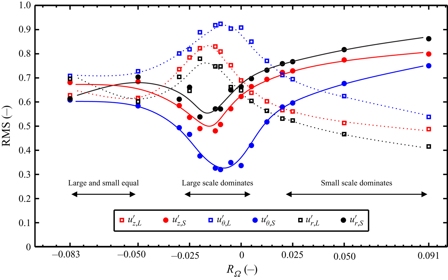
Figure 2. The r.m.s. of fluctuating large- and small-scale velocities versus  $R_{\varOmega }$ at $Re_S = 29\,000$. $u_z'$, $u_{\theta }'$ and $u_r'$ represent the fluctuating velocities in the axial, azimuthal and the radial directions, respectively. The second indices $L$ and $S$ (e.g. $u_{z,L}'$ and $u_{z,S}'$) represent the large- and smaller-scale components of the fluctuating velocity, respectively. The lines are included to guide the eye. The r.m.s. of fluctuating large- and small-scale velocities are normalized using the r.m.s. of the non-filtered fluctuations of each velocity component, e.g. $u_z'$. Horizontal arrows indicate the dominant scale in the different ranges of the rotation number.
Not only does the relative energy of the large scales change with rotation number, so does the orientation of the large-scale vortices. Since both the mean  $\boldsymbol {U}$, and the large-scale fluctuations $\boldsymbol {u}_L'$ showed roll structures, we combined these fields, i.e. ( $\boldsymbol {U}+\boldsymbol {u}_L'$), when evaluating the large-scale vortices and the associated large-scale vorticity. This can be interpreted as $\boldsymbol {U}$ capturing the steady, azimuthally homogeneous part of the rolls, while $\boldsymbol {u}_L'$ contains the unsteadiness of the rolls as well as any deviations from homogeneity in the azimuthal direction. Within the ( $\boldsymbol {U}+\boldsymbol {u}_L'$) field, the large-scale vortices are detected using the $Q$-criterion (Hunt, Wray & Moin Reference Hunt, Wray and Moin1988), where $Q$ is the second invariant of the velocity gradient tensor. The employed threshold is $Q \geq 0.024$, which is non-dimensionalized using $U_{sh}^2 / d^2$. Furthermore, the direction of the vorticity vector within these structures is taken as a measure for the orientation of the vortices. Figure 3 presents the statistical distribution of the orientation of the vortices for different $R_{\varOmega }$, where the angles $\beta$ and $\phi$ are defined in the inset of figure 3(d). Please note that all data points within the detected structures have been included in the statistics of $\beta$ and $\phi$. The results show profound changes in the orientation of the vortices. At large negative rotation number ( $R_{\varOmega } = -0.083$, figure 3a), the vortices are approximately aligned in the azimuthal direction ( $\beta \approx \pm 90^{\circ }$) and inclined with the cylinder walls at predominantly $25^{\circ }$. The two peaks in the joint probability-density-function (p.d.f.) correspond to counter-rotating vortex pairs. Because the vortices occur in pairs, the height of the two peaks is expected to be equal. However, in figure 3(a) the peak heights are different due to the limited measurement domain, which captures only three vortices, that is, one pair plus a half-pair. At $R_{\varOmega }= -0.010$ (figure 3b), which is near the condition for optimum angular momentum transport, the inclination angle increases and attains a wider distribution, where $| \phi |$ varies mostly between 20 and $60^{\circ }$. The distribution for the angles widens even more when the cylinders are in exact counterrotation (figure 3c), which marks the transition from azimuthally aligned vortices at negative $R_{\varOmega }$, to axially aligned vortices at positive $R_{\varOmega }$ (
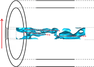
 $\beta = \phi = 0$, figure 3d). Some typical examples of the associated instantaneous vortical structures are shown in figure 4 by means of $Q$ iso-surfaces. Consistent with the statistical results in figure 3, the axes of the vortices are initially at shallow angles with respect to the walls (figure 4a). These structures are analogous to Taylor vortices, which were observed in the time-averaged flow at similar $R_{\varOmega }$ (Dong Reference Dong2007; Ravelet et al. Reference Ravelet, Delfos and Westerweel2010; Tokgoz et al. Reference Tokgoz, Elsinga, Delfos and Westerweel2012; Ostilla et al. Reference Ostilla, Stevens, Grossmann, Verzicco and Lohse2013). As the rotation number increases, the vortices become more inclined as the condition of optimal angular momentum is approached (figure 4b). The broad distribution of the angles in figure 3(c) is associated with ‘blob-like’ structures for $Q$ (figure 4c). At positive rotation numbers, the vortex axes are aligned in the axial direction and column-like (figure 4d). Maretzke, Hof & Avila (Reference Maretzke, Hof and Avila2014) associated finite columnar structures with optimal transient growth modes in laminar TC at similar rotation numbers. However, it has remained unclear whether columnar vortices could be seen at fully turbulent conditions (Tuckerman Reference Tuckerman2014). The present findings suggest they represent the large-scale flow structure at $R_{\varOmega } > 0$.
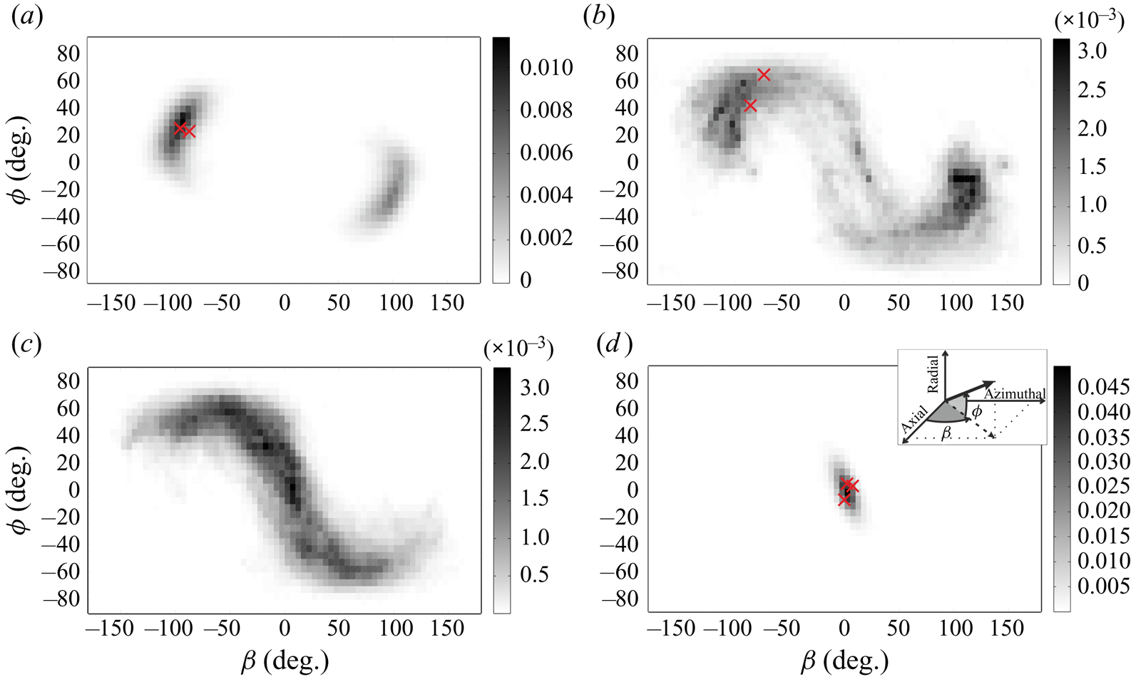
Figure 3. Joint-PDF of the orientation of the vorticity vector in the large-scale vortices for  $R_{\varOmega }=-0.083$ $(a)$, $-0.010$ $(b)$, $0$
$0$ $(c)$ and $0.091$ $(d)$. $Re_S = 29\,000$ for all cases. The angles $\beta$ and $\phi$ are with respect to the TC coordinate system as shown in $(d)$. For reference, $\phi = 0$, $\beta = {\pm }90^{\circ }$ corresponds to alignment in azimuthal direction, which coincides with the orientation of a pair of Taylor vortices, $\phi =0$, $\beta = {\pm } 90^{\circ } +\theta$ corresponds to spiral vortices inclined at an angle $\theta$ with respect to the azimuthal direction and $\phi = 0$, $\beta = 0$ corresponds to alignment in axial direction. Furthermore, red symbols ( $\times$) mark the orientation of the vortex axes as shown in the corresponding plots in figure 4.

Figure 4. Examples of instantaneous large-scale vortical structures at  $Re_S = 29\,000$ for $R_{\varOmega }=-0.083$ $(a)$, $-0.010$ $(b)$, $0$
$0$ $(c)$ and $0.091$ $(d)$. The iso-surfaces show $Q = 0.024$. Panels (a–c) show projections onto the azimuthal–radial plane, while $(d)$ shows the projection on the azimuthal–axial plane. $U_i$ and $U_o$ indicate the velocity of the inner and outer cylinder walls, respectively. The red dashed-lines (in a,b,d) indicate the axes of the vortical structures, which have been determined visually. Note that the blobs in $(c)$ do not reveal a principal axis.
In order to better understand the formation of columnar vortices, the Rossby number,  $Ro= \mathcal {U} / 2 \varOmega \mathcal {L}$, is evaluated. Here, $\varOmega =2 {\rm \pi}f_o$ is the angular velocity of the rotation, while $\mathcal {U}$ and $\mathcal {L}$ are the large-scale turbulent velocity and length scale respectively. In the bulk of a wall-bounded turbulent shear flow, the r.m.s. of the fluctuating velocity is of order $5\,\%$ of the velocity difference across the layer, which yields $\mathcal {U} \approx 0.05 \times 2 {\rm \pi}| f_i-f_o | r_i$ for TC flow. The length scale of interest is the gap width, i.e. $\mathcal {L}=d$. For the case of outer cylinder rotation only, $R_{\varOmega }= 0.091$, it follows that $Ro = 0.275$. Such a small Rossby number suggests that the Coriolis force dominates over inertial forces. At similar $Ro$, columnar vortical structures have been shown to form in DNS of homogenous rotating turbulence without walls (e.g. Yoshimatsu, Midorikawa & Kaneda Reference Yoshimatsu, Midorikawa and Kaneda2011). Therefore, the present columnar vortices are consistent with general turbulence at $Ro < 1$. Finite size or end effects are not necessary to explain the existence of columnar vortices in the TC gap.
The observed transitions in the orientation of the large-scale vortical structures (figures 3 and 4) have important implications for the Reynolds shear stress, as shown in figure 5. For  $R_{\varOmega } < -0.025$, the Reynolds shear stress in the bulk, hence the torque, is dominated by the mean flow contribution. At these conditions, the large-scale vortices are approximately aligned in the azimuthal direction and can be considered as steady Taylor vortices. However, beyond the conditions for optimal angular momentum transfer, i.e. $R_{\varOmega } \cong -0.02$, the large-scale vortices become more inclined with respect to the azimuthal direction (e.g. figure 4b), which reduces their contribution to the mean flow because of azimuthal averaging. These large-scale vortices induce a fluctuating velocity perpendicular to the vortex axis, which means they induce both ${u'}_{\theta ,L}$ and ${u'}_{r,L}$ at the same location, which explains their large correlation, that is their large Reynolds shear stress contribution $\overline {u'_{\theta ,L} u'_{r,L}}$. For positive $R_{\varOmega }$, the orientation of the large-scale vortices changes to the axial direction. In that case, ${u'}_{\theta ,L}$ and ${u'}_{r,L}$ are induced at different locations relative to the vortex, hence their correlation $\overline {u'_{\theta ,L} u'_{r,L}}$ diminishes. As a result, the small scales contribute most to the Reynolds shear stress beyond $R_{\varOmega }= +0.025$ (figure 5).

Figure 5. Contributions to the friction factor  $C_f$ associated with the mean flow and the instantaneous large-scale (LS) and smaller-scale (SS) velocity fluctuations in the TC gap at $Re_S = 29\,000$. Their combined total (circles) is compared against the estimated based on the torque measurements of Ravelet et al. (Reference Ravelet, Delfos and Westerweel2010) (triangles). The dashed lines are indicative of the trend in the data.
Finally, the friction coefficient determined from the total Reynolds shear stress in the core is compared with the  $C_f$ determined from the torque measurement (figure 5). The two approaches are generally consistent meaning that the PIV measurement captured the main effects. The differences may be explained by limited spatial resolution in PIV, which causes an underestimation of the small-scale fluctuations and their Reynolds shear stress contributions (Tokgoz et al. Reference Tokgoz, Elsinga, Delfos and Westerweel2012). At negative $R_{\varOmega }$, the small scales contribute relatively little to the overall torque, and the methods agree to within $6\,\%$. However, at positive $R_{\varOmega }$, the small-scale contribution is significant, and the relative difference increases to approximately $33\,\%$. Furthermore, the uncertainty in the contribution from the von Kármán gaps between the cylinder end plates to the torque as measured with the torque sensor may contribute to the observed differences.
4. Conclusion
With increasing rotation number, we found the large-scale flow structure to transition from steady Taylor rolls, to unsteady vortical structures inclined with respect to the wall, to columnar vortical structures aligned in the axial direction. These transitions in structure coincide with the transitions in the torque scaling and angular momentum transfer. The decay of the Taylor vortices in the mean flow does not coincide with the decay in the torque, and they occur at different rotation numbers (approximately  $R_{\varOmega } = -0.025$ and $0$ respectively, see figure 5). Therefore, Taylor vortices cannot fully explain the changes in the torque scaling near the conditions of optimal angular momentum transfer.
For sufficiently negative rotation number, it is the mean flow that is largely responsible for the torque, not the turbulence (i.e. the fluctuations).
The unsteady inclined vortical structures at intermediate rotation number induce  ${u'}_{\theta ,L}$ and ${u'}_{r,L}$ simultaneously. Hence, these velocity components are highly correlated, which implies large angular momentum transfer. ‘Optimum’ angular momentum transfer in our system is associated with the transition from the steady vortices to these unsteady vortices inclined at $45^{\circ }$ with the wall. The (steady) Taylor rolls alone are not optimal in transferring angular momentum.
At large positive rotation number, the axial vortices induce  ${u'}_{\theta ,L}$ and ${u'}_{r,L}$ in different places, hence little correlation or angular momentum transfer is produced. The Rossby number at these conditions is smaller than one indicating that the turbulence is rotation dominated and that columnar vortices are expected. Columnar structures in TC flow have been reported for transition (Maretzke et al. Reference Maretzke, Hof and Avila2014). However, they were not observed before for fully turbulent conditions. The detection of columnar vortices was first made possible by the volumetric velocity fields provided by tomographic-PIV.
Acknowledgements
In memoriam of Professor B. Eckhardt who passed away on August 7, 2019. We greatly appreciate his companionship and involvement in this work, and his suggestions and comments regarding earlier versions of this manuscript. The authors thank the Netherlands Foundation of Scientific Research Institutes (NWO-I) for their financial support through the programme 142 ‘Towards ultimate turbulence’ coordinated by Professor Lohse from the Physics of Fluids group at the University of Twente.
Declaration of interests
The authors report no conflict of interest.


 Open access