


1. Introduction
A defining feature of turbulent flows is the generation of small-scale structures, leading to dramatic enhancement of transport rates of mass, momentum and energy. In this regard, the importance of statistical properties of the velocity gradient tensor  ${\boldsymbol {A}} = \boldsymbol {\nabla } {\boldsymbol {u}}$, where
  ${\boldsymbol {u}}$ is the velocity field, is well recognized (Frisch Reference Frisch1995; Sreenivasan & Antonia Reference Sreenivasan and Antonia1997; Falkovich, Gawdzki & Vergassola Reference Falkovich, Gawdzki and Vergassola2001; Tsinober Reference Tsinober2009; Wallace Reference Wallace2009; Meneveau Reference Meneveau2011). By taking the derivative of the incompressible Navier–Stokes equations, the dynamics of
  ${\boldsymbol {A}}$ are given by the following transport equation:
 \begin{equation} \frac{{\rm D}A_{ij}}{{\rm D}t} ={-} A_{ik} A_{kj} - H_{ij} + \nu \nabla^2 A_{ij}, \end{equation}
where  ${\rm D}/{\rm D}t$ is the material derivative,
  $\nu$ is the kinematic viscosity,
  $H_{ij} = \partial ^2 P/\partial x_i \partial x_j$ is the pressure Hessian tensor; and the incompressibility condition imposes
  $A_{ii} = 0$. The quadratic nonlinearity in (1.1) captures the self-amplification of velocity gradients, which leads to intermittent generation of extreme events and small-scale structures in the flow. Owing to their practical significance in various physical processes (Falkovich, Fouxon & Stepanov Reference Falkovich, Fouxon and Stepanov2002; Hamlington, Poludnenko & Oran Reference Hamlington, Poludnenko and Oran2012; Buaria, Sawford & Yeung Reference Buaria, Sawford and Yeung2015; Voth & Soldati Reference Voth and Soldati2017; Buaria et al. Reference Buaria, Clay, Sreenivasan and Yeung2021), their postulated universality (Kolmogorov Reference Kolmogorov1941; Frisch Reference Frisch1995; Sreenivasan & Antonia Reference Sreenivasan and Antonia1997), as well as their connection to potential singularities of the Euler and Navier–Stokes equations (Gibbon, Bustamante & Kerr Reference Gibbon, Bustamante and Kerr2008; Doering Reference Doering2009; Fefferman Reference Fefferman2006), the study of small scales and velocity gradients is of obvious importance in turbulence theory and modelling.
As implied by (1.1), the dynamics of velocity gradients are influenced by the pressure Hessian tensor. This leads to a non-local coupling of the entire gradient field, since pressure satisfies the Poisson equation,  $\nabla ^2 P = - A_{ij} A_{ji}$, as obtained by taking the trace of (1.1). The mathematical difficulties posed by this non-locality make it very hard to decipher the precise role of the pressure Hessian on gradient amplification and the formation of extreme events. In general, it has been observed that the pressure Hessian acts to counteract the nonlinear amplification (Nomura & Post Reference Nomura and Post1998; Kalelkar Reference Kalelkar2006; Tsinober Reference Tsinober2009; Lawson & Dawson Reference Lawson and Dawson2015; Carbone, Iovieno & Bragg Reference Carbone, Iovieno and Bragg2020; Buaria, Pumir & Bodenschatz Reference Buaria, Pumir and Bodenschatz2022). Since the pressure Hessian is a symmetric tensor, its influence on the amplification of strain-rate (with ‘rate’ omitted hereafter for brevity, as in common usage), the symmetric part of the
  ${\boldsymbol {A}}$, is more explicit (Nomura & Post Reference Nomura and Post1998; Buaria, Pumir & Bodenschatz Reference Buaria, Pumir and Bodenschatz2020b). In contrast, its influence on vorticity, the skew-symmetric part of
  ${\boldsymbol {A}}$, is indirectly felt through strain, and much more difficult to understand. The interaction between vorticity and strain itself is an indispensable ingredient of turbulence. For instance, it is well established that vorticity preferentially aligns with the eigenvector corresponding to the intermediate eigenvalue of the strain tensor, which in turn is positive on average (Ashurst et al. Reference Ashurst, Kerstein, Kerr and Gibson1987; Tsinober Reference Tsinober2009). Additionally, this alignment is considerably stronger in regions of intense vorticity and strain (Buaria, Bodenschatz & Pumir Reference Buaria, Bodenschatz and Pumir2020a; Buaria et al. Reference Buaria, Pumir and Bodenschatz2022). In contrast, the role of pressure Hessian, especially in regions of intense vorticity or strain has received little or no attention.
Prior studies predominantly focused on unconditional statistics, which do not distinguish quiescent regions from regions where extreme events reside. Additionally, they have also been restricted to low Reynolds numbers (Nomura & Post Reference Nomura and Post1998; Tsinober, Ortenberg & Shtilman Reference Tsinober, Ortenberg and Shtilman1999; Lawson & Dawson Reference Lawson and Dawson2015). It is well known that extreme vorticity and strain events in turbulence have a pronounced structure, where the statistical properties can be very different than the mean field (Jiménez et al. Reference Jiménez, Wray, Saffman and Rogallo1993; Moisy & Jiménez Reference Moisy and Jiménez2004; Tsinober Reference Tsinober2009; Buaria et al. Reference Buaria, Bodenschatz and Pumir2020a, Reference Buaria, Pumir and Bodenschatz2022). Thus, analysing statistics conditioned on the magnitude of vorticity or strain can be particularly useful to understand the underlying amplification mechanism (Tsinober Reference Tsinober2009; Buaria et al. Reference Buaria, Bodenschatz and Pumir2020a, Reference Buaria, Pumir and Bodenschatz2022). In addition to providing fundamental insights, conditional statistics of the pressure Hessian also play a central role in turbulence modelling, particularly Lagrangian modelling of velocity gradient dynamics (Girimaji & Pope Reference Girimaji and Pope1989; Meneveau Reference Meneveau2011; Lawson & Dawson Reference Lawson and Dawson2015; Tian, Livescu & Chertkov Reference Tian, Livescu and Chertkov2021; Buaria & Sreenivasan Reference Buaria and Sreenivasan2023a; Johnson & Wilczek Reference Johnson and Wilczek2023).
In this work, our objective is to systematically analyse the effect of pressure Hessian on amplification of vorticity and strain. We identify and analyse various correlations between the pressure Hessian and vorticity and strain fields. We consider unconditional statistics and also statistics conditioned on the magnitude of vorticity and strain, to focus on extreme events. It is worth noting that strain itself can be non-locally related to vorticity, via the Biot–Savart integral, providing an alternative way to study the non-locality of gradient amplification – without invoking pressure – by filtering strain into scalewise contributions (Hamlington, Schumacher & Dahm Reference Hamlington, Schumacher and Dahm2008; Buaria et al. Reference Buaria, Pumir and Bodenschatz2020b; Buaria & Pumir Reference Buaria and Pumir2021). Alternatively, the pressure Hessian tensor itself can also be filtered into scalewise contributions (Vlaykov & Wilczek Reference Vlaykov and Wilczek2019). Complementary to these approaches, our focus here is to directly analyse the pressure Hessian term to directly investigate its role on gradient amplification.
To that end, the necessary statistics are extracted from state-of-the-art direct numerical simulations of isotropic turbulence in periodic domains, which is the most efficient numerical tool to study the small-scale properties of turbulence. One important purpose of the current study is also to understand the effect of increasing Reynolds number. To this end, we utilize a massive direct numerical simulations (DNS) database with Taylor-scale Reynolds number  ${R_\lambda }$ ranging from
  $140$ to
  $1300$, on up to grid sizes of
  $12\,288^3$; particular attention is given on having good small-scale resolution to accurately resolve the extreme events (Buaria et al. Reference Buaria, Pumir, Bodenschatz and Yeung2019, Reference Buaria, Bodenschatz and Pumir2020a, Reference Buaria, Pumir and Bodenschatz2022), for which conditional statistics are analysed.
The manuscript is organized as follows. The necessary background for our analysis is briefly reviewed in § 2. The numerical approach and DNS database is presented in § 3. In § 4, the role of pressure Hessian is analysed in the context of vorticity amplification, whereas in § 5 the analysis is in the context of strain amplification. Finally, we summarize our results in § 6.
2. Background
The vorticity vector  ${\boldsymbol {\omega }}$ and the strain tensor
  ${\boldsymbol {S}}$, defined as
  $\omega _i=\varepsilon _{ijk} A_{jk}$ (
 $\varepsilon _{ijk}$ being the Levi–Civita symbol) and
  $S_{ij} = (A_{ij} + A_{ji})/2$, represent the skew-symmetric and symmetric components of the velocity gradient tensor, respectively, and characterize the local rotational and stretching motions. Their evolution equations can be readily obtained from (1.1) and are given as
 $$\begin{gather} \frac{{\rm D} \omega_i}{{\rm D}t} = \omega_j S_{ij} + \nu \nabla^2 \omega_i , \end{gather}$$
 $$\begin{gather}\frac{{\rm D} S_{ij}}{{\rm D}t} ={-}S_{ik} S_{kj} - \frac{1}{4} (\omega_i \omega_j - \omega^2 \delta_{ij}) - H_{ij} + \nu \nabla^2 S_{ij} . \end{gather}$$
The nonlinear amplification of vorticity is captured by the vortex stretching vector  $W_i = \omega _j S_{ij}$, whereas amplification of strain is controlled by the self-amplification term and additionally via feedback of vorticity. Although the pressure Hessian, which is a symmetric tensor, only contributes to evolution of strain, it still indirectly affects vorticity, since the pressure Poisson couples both vorticty and strain. Indeed, taking the trace of (2.2), gives
  $\nabla ^2 P = (\omega _i \omega _i - 2 S_{ij} S_{ij})/2$. The influence of pressure Hessian on vorticity becomes apparent when considering the evolution equation for the vortex stretching vector,
 \begin{equation} \frac{{\rm D} W_i}{{\rm D}t} ={-} \omega_j H_{ij} + \text{viscous terms} . \end{equation}
Note that  ${\rm D} W_i/{\rm D}t = {\rm D}^2 \omega _i /{\rm D}t^2$ in the inviscid limit, which directly relates the pressure Hessian to the second derivative of vorticity.
To quantify the intensity of gradients, we consider the magnitudes of vorticity and strain (Buaria et al. Reference Buaria, Pumir, Bodenschatz and Yeung2019; Buaria & Pumir Reference Buaria and Pumir2022)
 \begin{equation} \varOmega = \omega_i \omega_i , \quad \varSigma = 2 S_{ij} S_{ij} , \end{equation}
where the former is the enstrophy, and the latter is dissipation rate  $\epsilon$ divided by viscosity, i.e.
  $\varSigma = \epsilon / \nu$. In homogeneous turbulence,
  $\langle \varOmega \rangle = \langle \varSigma \rangle = 1/\tau _K^2$, where
  $\tau _K$ is the Kolmogorov time scale. Likewise, it is useful to consider transport equations for these quantities,
 $$\begin{gather} \frac{1}{2} \frac{{\rm D} \varOmega }{{\rm D}t} = \omega_i \omega_j S_{ij} + \nu \omega_i \nabla^2 \omega_i , \end{gather}$$
 $$\begin{gather}\frac{1}{4} \frac{{\rm D} \varSigma}{{\rm D}t} ={-}S_{ij} S_{jk} S_{ki} - \frac{1}{4} \omega_i \omega_j S_{ij} - S_{ij} H_{ij} + \nu S_{ij} \nabla^2 S_{ij}. \end{gather}$$
The amplification of enstrophy is engendered by the term  $\omega _i \omega _j S_{ij} = \omega _i W_i$, which in turn evolves according to
 \begin{equation} \frac{{\rm D} \omega_i W_i }{{\rm D}t} = W_i W_i - \omega_i \omega_j H_{ij} + \text{viscous terms} . \end{equation}
In the inviscid limit,  ${\rm D} (\omega _i W_i)/{\rm D}t = {\rm D}^2 \varOmega /{\rm D}t^2$, thus (2.7) is complementary to (2.3) for
  $W_i$. The above equations identify the correlations responsible for generation of intense velocity gradients, which we will analyse, both unconditionally and conditioned on magnitudes of
  $\varOmega$ and
  $\varSigma$.
For our analysis, it is also useful to consider the eigenframes of the strain and pressure Hessian tensors. For the strain tensor, it is defined by the eigenvalues  $\lambda _i$ (for
  $i=1,2,3$), such that
  $\lambda _1 \geqslant \lambda _2 \geqslant \lambda _3$ and the corresponding eigenvectors
  $\boldsymbol {e}_i$. Incompressibility gives
  $\lambda _1 + \lambda _2 + \lambda _3=0$, implying that
  $\lambda _1$ is always positive (stretching) and
  $\lambda _3$ is always negative (compressive). Similarly, the eigenframe of pressure Hessian is given by the eigenvalues
  $\lambda _i^{P}$ (in descending order), and eigenvectors
  $\boldsymbol {e}_i^{P}$. In this case, incompressibility gives
  $H_{ii} = \nabla ^2 P = \lambda _1^{P} + \lambda _2^{P} + \lambda _3^{P}$, which is in general non-zero. Thus, it is convenient to decompose the pressure Hessian into isotropic and deviatoric components,
 $$\begin{gather} H_{ij}^{I} = \frac{H_{kk}}{3} \delta_{ij} ,\quad \text{with} \ H_{kk} = \nabla^2 P = (\varOmega - \varSigma)/2 , \end{gather}$$
 $$\begin{gather}H_{ij}^{D} = H_{ij} - H_{ij}^{I} . \end{gather}$$
Note that since  ${\boldsymbol {H}}^{I}$ can be explicitly expressed in terms of
  ${\boldsymbol {A}}$, it can be considered local, whereas
  ${\boldsymbol {H}}^{D}$ captures the non-locality of the pressure field since it requires explicit solution to the Poisson equation (Ohkitani & Kishiba Reference Ohkitani and Kishiba1995). In principle, strain is itself non-locally related to vorticity in incompressible flows, via the Biot–Savart relation (Hamlington et al. Reference Hamlington, Schumacher and Dahm2008; Buaria et al. Reference Buaria, Pumir and Bodenschatz2020b); but in the context of the pressure field, velocity gradients can be nominally interpreted as local. The eigenvalues
  $\lambda _i^{D}$ of
  $H_{ij}^{D}$ satisfy
 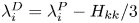 $\lambda _i^{D} = \lambda _i^{P} - H_{kk}/3$ and hence,
  $\lambda _1^{D} + \lambda _2^{D} + \lambda _3^{D} = 0$, implying
  $\lambda _1^{D} >$ and
  $\lambda _3^{D} <0$; whereas the eigenvectors are unaffected, i.e.
  $\boldsymbol {e}_i^{D} = \boldsymbol {e}_i^{P}$. Using this framework, we obtain
 \begin{align} \omega_i \omega_j H_{ij} = \lambda_i^{P} (\boldsymbol{e}_i^{P} \boldsymbol{\cdot} {\boldsymbol{\omega}})^2 ,\quad \omega_i \omega_j H_{ij}^{D} = \lambda_i^{D} (\boldsymbol{e}_i^{P} \boldsymbol{\cdot} {\boldsymbol{\omega}})^2 ,\quad \omega_i \omega_j H_{ij}^{I} = \varOmega (\varOmega - \varSigma)/6 , \end{align}
which decomposes the correlation between vorticity and the pressure Hessian into individual contributions from each eigendirection. Similarly, the terms  $\omega _i W_i$ and
  $W_i W_i$ can be decomposed in the eigenframe of the strain tensor, illustrating the importance of the alignments between vorticity vector and the eigenvectors of strain. We refer to our recent works (Buaria et al. Reference Buaria, Bodenschatz and Pumir2020a, Reference Buaria, Pumir and Bodenschatz2022) for a discussion of these properties, On the other hand, the contribution
  $S_{ij} H_{ij}$ in (2.6) can be written as
 \begin{equation} S_{ij} H_{ij} = \lambda_i^{P} \lambda_j (\boldsymbol{e}_i^{P} \boldsymbol{\cdot} \boldsymbol{e}_j )^2 . \end{equation}
Since,  $S_{ij} H_{ij}^{I} = 0$ from incompressibility, it also follows that
 \begin{equation} S_{ij} H_{ij} = S_{ij} H_{ij}^{D} = \lambda_i^{D} \lambda_j (\boldsymbol{e}_i^{P} \boldsymbol{\cdot} \boldsymbol{e}_j )^2 . \end{equation}
3. Numerical approach and database
The data utilized here are the same as in several recent works (Buaria & Sreenivasan Reference Buaria and Sreenivasan2020; Buaria et al. Reference Buaria, Bodenschatz and Pumir2020a,Reference Buaria, Pumir and Bodenschatzb; Buaria & Pumir Reference Buaria and Pumir2021; Buaria & Sreenivasan Reference Buaria and Sreenivasan2022a, Reference Buaria and Sreenivasan2023b) and are generated using DNS of incompressible Navier–Stokes equations, for the canonical set-up of isotropic turbulence in a periodic domain. The simulations are carried out using highly accurate Fourier pseudospectral methods with second-order Runge–Kutta integration in time, and the large scales are forced numerically to achieve statistical stationarity (Rogallo Reference Rogallo1981). A key characteristic of our data is that we have achieved a wide range of Taylor-scale Reynolds number  ${R_\lambda }$, going from 140–1300, while maintaining excellent small-scale resolution, which is as high as
  $k_{\rm max} \eta \approx 6$, where
  $k_{max} = \sqrt {2}N/3$, is the maximum resolved wavenumber on a
  $N^3$ grid, and
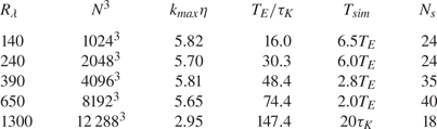
  $\eta$ is the Kolmogorov length scale. Convergence with respect to resolution and statistical sampling has been adequately established in previous works. For convenience, we summarize the DNS database and the simulation parameters in table 1; additional details can be obtained in our prior works cited earlier.
Table 1. Simulation parameters for the DNS runs used in the current work: the Taylor-scale Reynolds number ( ${R_\lambda }$); the number of grid points (
 $N^3$); spatial resolution (
 $k_{max}\eta$); ratio of large-eddy turnover time (
 $T_E$) to Kolmogorov time scale (
 $\tau _K$); length of simulation (
 $T_{sim}$) in statistically stationary state; the number of instantaneous snapshots (
 $N_s$) used for each run to obtain the statistics.
4. Role of pressure Hessian on vorticity amplification
4.1. Unconditional statistics
Table 2 lists various unconditional statistics characterizing the role of the pressure Hessian on vortex stretching, based on (2.7), at different  ${R_\lambda }$. All quantities are appropriately non-dimensionalized by the Kolmogorov time scale
  $\tau _K$, and henceforth, should be interpreted as such (unless otherwise mentioned). We first consider the eigenvalues of the pressure Hessian. Owing to homogeneity
  $\langle H_{ii} \rangle = 0$; thus,
  $\sum _{i=1}^{3} \langle \lambda _i^{P} \rangle = 0$ and
  $\langle \lambda _i^{P} \rangle = \langle \lambda _i^{D} \rangle$. Table 2 reveals that the individual averages of the eigenvalues are approximately equal to
 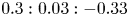 $0.3: 0.03: -0.33$, without any appreciable dependence on
  ${R_\lambda }$. The intermediate eigenvalue is overall positive on average but its magnitude is substantially smaller than the other two, and essentially close to zero.
Table 2. Unconditional averages of various quantities associated with correlation of vorticity and pressure Hessian, based on (2.7). Here  $\lambda _i^{P}$, for
  $i=1,2,3$, are the eigenvalues of pressure Hessian, with corresponding eigenvectors
  $\boldsymbol {e}_i^{P}$. All quantities are appropriately normalized by the Kolmogorov time scale
  $\tau _K$.

Similarly, the mean square of alignment cosines between vorticity and eigenvectors of pressure Hessian,  $\langle (\boldsymbol {e}_i^{P} \boldsymbol {\cdot } \hat {{\boldsymbol {\omega }}})^2 \rangle$, where
  $\hat {{\boldsymbol {\omega }}}$ denotes the unit vector parallel to
  ${\boldsymbol {\omega }}$, are also essentially independent of
  ${R_\lambda }$. Note that the square of cosines sum up to unity for all three directions. Additionally, they are bounded between 0 and 1 for each individual direction, respectively, for the case of perfect orthogonal and parallel alignment; whereas for a uniform distribution of the alignment cosine, the mean square average is
  $1/3$. From table 2, we observe that the measured alignments do not deviate significantly from
  $1/3$, with a weak preferential alignment of vorticity with the intermediate eigenvector of the pressure Hessian.
It is worth noting that while a uniform distribution of the alignment cosine implies the second moment is  $1/3$, the reverse is not necessarily true. Thus, it is useful to also inspect the p.d.f. of the alignment cosines (Chevillard et al. Reference Chevillard, Meneveau, Biferale and Toschi2008), which are shown in figure 1. The solid and dashed curves correspond to
  ${R_\lambda }=1300$ and
  $140$, respectively, demonstrating that the alignments are independent of
  ${R_\lambda }$. The distributions for
  $|\boldsymbol {e}_1^{P} \boldsymbol {\cdot } \hat {{\boldsymbol {\omega }}}|$ and
  $|\boldsymbol {e}_1^{P} \boldsymbol {\cdot } \hat {{\boldsymbol {\omega }}}|$ conform with expectation from their second moments in table 2, indicating weak preferential orthogonal and parallel alignment, respectively. However, for
  $|\boldsymbol {e}_3^{P} \boldsymbol {\cdot } \hat {{\boldsymbol {\omega }}}|$, we observe an anomalous behaviour, showing simultaneous preferential orthogonal and parallel alignments, which cancel each other out when evaluating the second moment. Note that the limiting cases of 0 or 1 for the second moment of alignment cosines do not present such an anomaly for the p.d.f.s. In fact, we will see later that when considering conditional statistics, the alignments are substantially enhanced for extreme vorticity events (such that using the second moment only does not lead to any ambiguity).

Figure 1. Probability density function (p.d.f.) of alignment cosines between vorticity and eigenvectors of pressure Hessian at  ${R_\lambda }=1300$ (solid lines) and
  ${R_\lambda }=140$ (dashed lines).
Finally, we consider the net contributions to the budget of vortex stretching (as per (2.7)). Table 2 shows separately the mean contributions from the deviatoric and isotropic components of the pressure Hessian and their sum  $\langle \omega _i \omega _j H_{ij} \rangle$, contrasted with the nonlinear term
  $\langle W_i W_i \rangle$. Remarkably, the deviatoric and isotropic contributions are comparable in magnitude, but opposite in sign. Taking into account the negative sign before the pressure Hessian term in (2.7), it follows that
  ${\boldsymbol {H}}^{D}$ favours vortex stretching, whereas
  ${\boldsymbol {H}}^{I}$ inhibits it. This essentially establishes that non-local effects of the pressure field enable vortex stretching (Ohkitani & Kishiba Reference Ohkitani and Kishiba1995). This also conforms with non-locality of vortex stretching as highlighted in recent studies (Hamlington et al. Reference Hamlington, Schumacher and Dahm2008; Buaria & Pumir Reference Buaria and Pumir2021); however, it is worth noting that the non-locality in these studies was investigated in the context of the Biot–Savart relation between vorticity and strain. We will further elaborate on this connection later.
The strong cancellation between the deviatoric and isotropic contributions results in a weakly positive value of  $\langle \omega _i \omega _j H_{ij} \rangle$, implying that pressure Hessian overall weakly opposes vortex stretching – which is primarily a local effect stemming from the dominant isotropic contribution of pressure Hessian. Both the deviatoric and isotropic contributions become stronger with
  ${R_\lambda }$, but the latter is always slightly stronger. In contrast, the term
  $\langle W_i W_i\rangle$, also given in table 2, is positive by definition, and thus always enables vortex stretching. This term increases with
  ${R_\lambda }$ and is noticeably larger than
  $\langle \omega _i \omega _j H_{ij} \rangle$ (at all
  ${R_\lambda }$). This leads to the (anticipated) result that the nonlinear effects in turbulence predominantly enable vortex stretching, with a net positive energy cascade from large to small scales (Batchelor Reference Batchelor1953; Betchov Reference Betchov1956; Kerr Reference Kerr1985). Although not shown, the
  ${R_\lambda }$ dependence of these quantities conforms with an approximate power law of
  $R_\lambda ^{0.39}$ in nominal agreement with fourth-order moment of velocity derivatives (Gylfason, Ayyalasomayjula & Warhaft Reference Gylfason, Ayyalasomayjula and Warhaft2004; Buaria & Sreenivasan Reference Buaria and Sreenivasan2022b).
4.2. Conditional statistics
In the previous subsection, we considered unconditional statistics, which provide an overall global perspective of the flow. To specifically characterize the extreme events or regions of intense vorticity, we condition the statistics on the magnitude of vorticity; specifically, we will use  $\varOmega \tau _K^2$ (or equivalently,
  $\varOmega /\langle \varOmega \rangle$), to quantify the extremeness of an event with respect to the mean field.
Figure 2 shows the conditional mean square of alignment cosines between vorticity and the eigenvectors of pressure Hessian, at various  ${R_\lambda }$. For weak enstrophy, all the curves are at
  $1/3$, consistent with a uniform distribution of cosines. For
  $\varOmega \tau _K^2 \approx 1$, we notice that vorticity has a weak preferential alignment with
  $\boldsymbol {e}^{P}_2$, in agreement with the unconditional results in table 2. However, for extreme events, a different picture emerges and vorticity almost perfectly aligns with
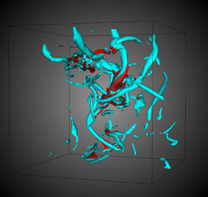
  $\boldsymbol {e}^{P}_3$ (becoming orthogonal to both first and second eigenvectors). This alignment can be explained by considering the familiar picture of intense vorticity being arranged in tube-like structures (Jiménez et al. Reference Jiménez, Wray, Saffman and Rogallo1993; Ishihara et al. Reference Ishihara, Kaneda, Yokokawa, Itakura and Uno2007; Buaria et al. Reference Buaria, Pumir, Bodenschatz and Yeung2019), as discussed at the end of the present subsection.
Figure 2. Conditional expectation (given enstrophy  $\varOmega$) of second moment of alignment cosines between vorticity unit vector (
 $\hat {{\boldsymbol {\omega }}}$) and eigenvectors of pressure Hessian (
 $\boldsymbol {e}_i^{P}$), at various
  ${R_\lambda }$.
Figure 3 shows the conditional expectation of the eigenvalues of pressure Hessian. To focus on extreme events, the abscissa is set to  $\varOmega \tau _K^2 \geqslant 1$. The identity
  $\sum _i \lambda _i^{P} = \nabla ^2 P = (\varOmega - \varSigma )/2$ implies that
 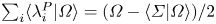 $\sum _i \langle \lambda _i^{P} | \varOmega \rangle = (\varOmega - \langle \varSigma |\varOmega \rangle )/2$. Recent numerical works (Buaria et al. Reference Buaria, Pumir, Bodenschatz and Yeung2019, Reference Buaria, Bodenschatz and Pumir2020a; Buaria & Pumir Reference Buaria and Pumir2022) have shown that for large enstrophy,
  $\langle \varSigma |\varOmega \rangle \sim \varOmega ^\gamma$, where the exponent
  $\gamma < 1$, but weakly increases with
  ${R_\lambda }$ (with
  $\gamma \to 1$ being the asymptotic limit). Thus, while the average sum of eigenvalues is zero for the mean field, it is strongly positive in regions of intense enstrophy. In fact, to the leading order, one can anticipate that
  $\langle \lambda _i^{P} | \varOmega \rangle \sim \varOmega$ when
  $\varOmega \tau _K^2 \gg 1$. Figure 3(a) shows the quantity
  $\langle \lambda _i^{P} | \varOmega \rangle / \varOmega$. The behaviour of the averaged eigenvalues at
  $\varOmega \tau _K^2 =1$ is consistent with the results in table 2. However, in regions of intense enstrophy, the first two eigenvalues are strongly positive, whereas the third eigenvalue is essentially zero. Once again, no appreciable dependence on
  ${R_\lambda }$ is seen for this case.
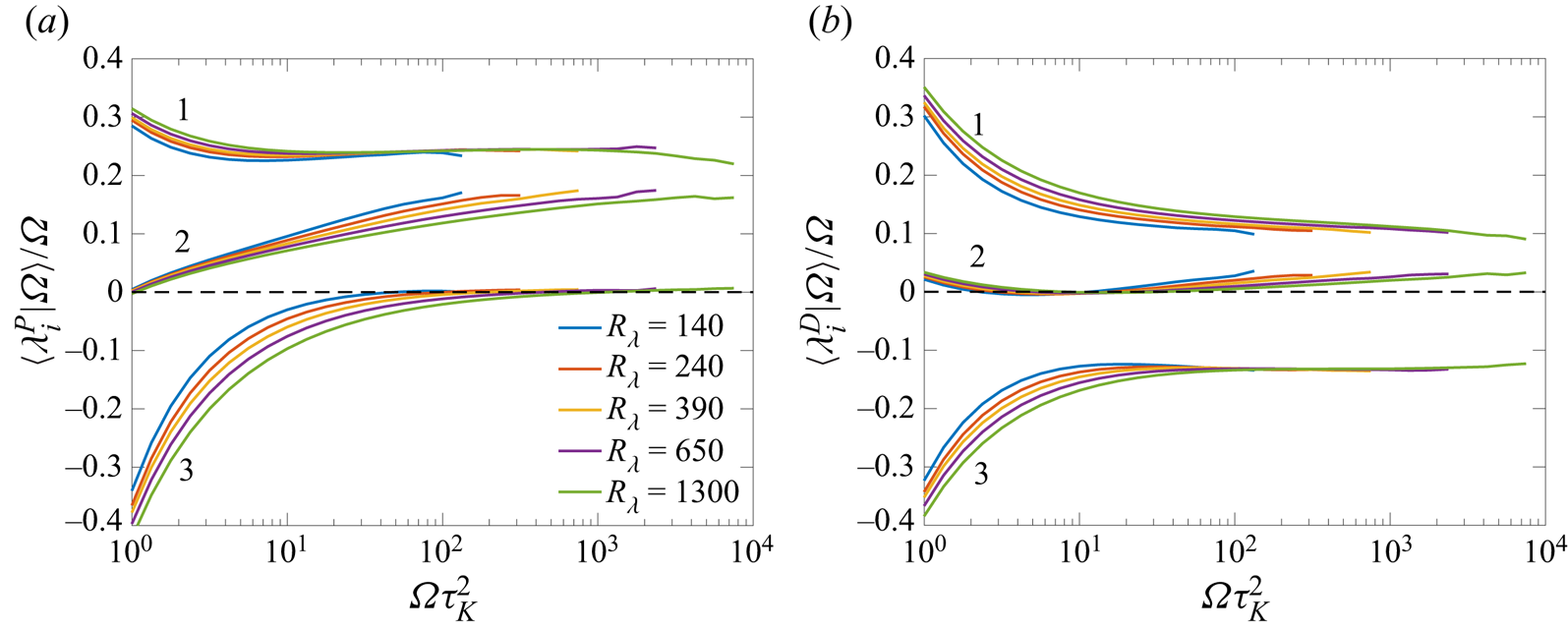
Figure 3. (a) Conditional expectations (given enstrophy  $\varOmega$) of the eigenvalues of pressure Hessian, for various
  ${R_\lambda }$. (b) Conditional expectations of the eigenvalues of the deviatoric part. The legend in panel (a) also applies to panel (b).
Given that vorticity is almost perfectly aligned with third eigenvector of the pressure Hessian and the corresponding eigenvalue is close to zero, the behaviour of the term  $\omega _i \omega _j H_{ij}$ cannot be easily inferred. Figure 4(a) shows the conditional expectation
  $\langle \omega _i \omega _j H_{ij} |\varOmega \rangle /\varOmega ^2$, along with the individual contributions in each eigendirection. The normalization by
  $\varOmega ^2$ comes from simple dimensional grounds. For
  $\varOmega \tau _K^2 \simeq 1$, the contributions from the first and third eigendirections are expectedly positive and negative, respectively, largely cancelling each other to give a weakly positive net contribution (whereas the contribution from second direction is essentially negligible). However, for
  $\varOmega \tau _K^2 \gg 1$, the contributions from all directions become positive and comparable. Thus, in regions of intense vorticity, the role of pressure (Hessian) is to oppose vortex stretching.
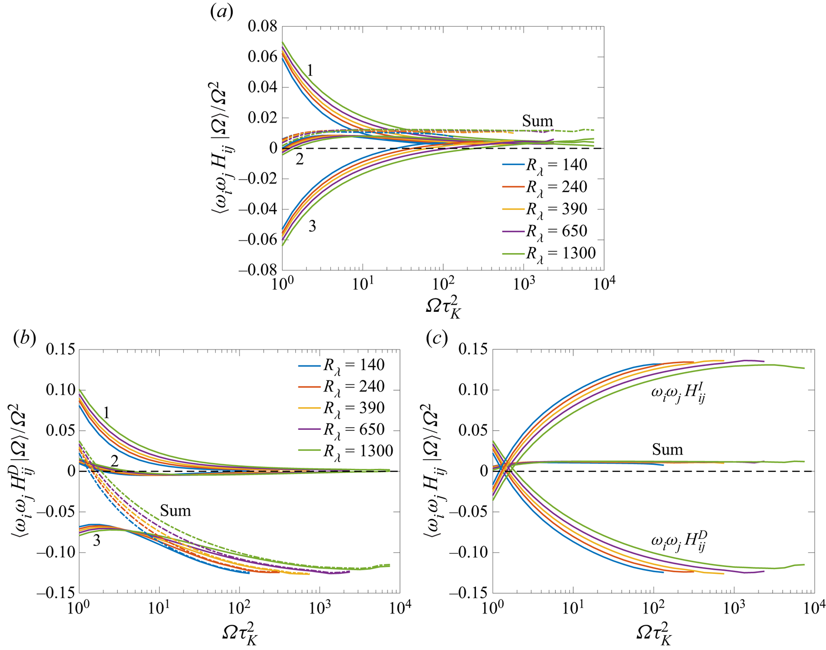
Figure 4. (a) Conditional expectation (given enstrophy  $\varOmega$) of the term
  $\omega _i \omega _j H_{ij}$ (marked as sum) and individual contributions from each eigendirection of pressure Hessian (in solid lines). The quantities are normalized by
  $\varOmega ^2$ to reveal a plateau-like behaviour for
  $\varOmega \tau _K^2 \gg 1$. (b) Same as panel (a), but for
  $\omega _i \omega _j H_{ij}^{D}$, (the contribution from the deviatoric part of pressure Hessian). (c) The net contributions from a and b are further contrasted with
  $\omega _i \omega _j H_{ij}^{I}$ (the contribution from isotropic part of pressure Hessian).
To better understand this result, we consider next the contributions from the deviatoric and the isotropic components of the pressure Hessian. The sum of eigenvalues of the deviatoric part  ${\boldsymbol {H}}^{D}$ is always constrained to be zero, i.e.
  $\sum _i \lambda _i^D = 0$, and thus,
  $\sum _i \langle \lambda _i^{D} | \varOmega \rangle = 0$. Figure 3(b) shows the conditional expectation
  $\langle \lambda _i^{D} | \varOmega \rangle / \varOmega$. While the results shown in figure 3(b) for
  $\varOmega \tau _K^2 \simeq 1$ are essentially identical to
  $\langle \lambda _i^P | \varOmega \rangle$, the behaviour for
  $\varOmega \tau _K \gg 1$ is different, with the first and second eigenvalues being always positive (with the second being noticeably weaker), whereas third eigenvalue is always negative (perfectly cancelling the contribution from other two). Thus, from the results in figures 2 and 3(b), it can be anticipated that
  $\langle \omega _i \omega _j H^{D}_{ij} |\varOmega \rangle$ is negative in regions of intense enstrophy. The contribution of the isotropic component is also easy to understand, since
  $\langle \omega _i \omega _j H^{I}_{ij} |\varOmega \rangle = \langle \varOmega (\varOmega - \varSigma ) |\varOmega \rangle /6 = (\varOmega ^2 - \varOmega \langle \varSigma |\varOmega \rangle )/6$. Using
  $\langle \varSigma |\varOmega \rangle \sim \varOmega ^\gamma$ (with
  $\gamma < 1$) implies that
  $\langle \omega _i \omega _j H^{I}_{ij} |\varOmega \rangle$ is positive in regions of intense enstrophy. We verify these expectations in figures 4(b) and 4(c).
Figure 4(b) shows the conditional expectation  $\langle \omega _i \omega _j H_{ij}^{D} |\varOmega \rangle /\varOmega ^2$, along with the individual contributions in each eigendirection. It can be clearly seen that for large enstrophy, the contributions from both first and second eigendirections are essentially zero and the third eigendirection completely dominates the overall sum (as explained earlier). This again establishes that the non-local portion of the pressure Hessian actually enables vortex stretching. In figure 4(c), we compare the contributions from the deviatoric and isotropic components, together with the overall average. We notice that the isotropic contribution is strongly positive, cancelling the deviatoric contribution to give a weakly net positive average. Once again, this shows that the depletion of vortex stretching by pressure Hessian is local.
It is worth noting that many qualitative aspects of the previously discussed results can be explained by noting that intense enstrophy is found in tube-like vortices (Jiménez et al. Reference Jiménez, Wray, Saffman and Rogallo1993; Ishihara et al. Reference Ishihara, Kaneda, Yokokawa, Itakura and Uno2007; Buaria et al. Reference Buaria, Pumir, Bodenschatz and Yeung2019), for which the Burgers vortex model is a good first-order approximation (Burgers Reference Burgers1948; Jiménez et al. Reference Jiménez, Wray, Saffman and Rogallo1993). For the simple case of a Burgers vortex, pressure is minimum and constant along the axis of the vortex. This implies that the smallest (third) eigenvalue of the pressure Hessian is zero and the corresponding eigenvector is perfectly aligned with vorticity; whereas the first two eigenvalues are positive and the corresponding eigenvectors are perfectly orthogonal to vorticity (Andreotti Reference Andreotti1997). Indeed, these expectations are qualitatively consistent with the results shown in figures 2 and 3. However, we note that the precise structure of vortices in turbulence is different than the Burgers vortex in some very crucial aspects. For instance, due to the structural properties of the Burgers vortex, the term  $\omega _i \omega _j H_{ij}$ is essentially zero, which is not the case in turbulence. Additionally, vorticity is perfectly axial in the Burgers vortex, but not real turbulent vortices, and there is some noticeable degree of Beltramization (Choi, Kim & Lee Reference Choi, Kim and Lee2009; Buaria et al. Reference Buaria, Pumir and Bodenschatz2020b) – an effect that is essential to the self-attenuation mechanism analysed in Buaria et al. (Reference Buaria, Pumir and Bodenschatz2020b) and Buaria & Pumir (Reference Buaria and Pumir2021). In fact, we will discuss in the next subsection that the net positive contribution from the pressure Hessian as observed in figure 4 is in fact connected to the self-attenuation mechanism observed in Buaria et al. (Reference Buaria, Pumir and Bodenschatz2020b) and Buaria & Pumir (Reference Buaria and Pumir2021).
4.3. Contrasting nonlinear and pressure Hessian contributions
Table 2 demonstrates that the (unconditional) contribution  $\langle W_i W_i \rangle$ is substantially larger than
  $\langle \omega _i \omega _j H_{ij}\rangle$ at all
  ${R_\lambda }$. A comparison of the conditional result is first made in figure 5(a). Evidently, the nonlinear term prevails over the pressure Hessian term at
  $\varOmega \tau _K^2 \simeq 1$, in essential agreement with the observation in table 2. However, for intense enstrophy, we notice a substantial reduction in the nonlinear term
  $\langle W_i W_i | \varOmega \rangle /\varOmega ^2$ relative to the pressure Hessian term
  $\langle \omega _i \omega _j H_{ij} | \varOmega \rangle /\varOmega ^2$, with the latter being approximately constant. Since
  $W_i = \omega _j S_{ij}$, it follows that
  $\langle W_i W_i |\varOmega \rangle \sim \langle \varOmega \varSigma |\varOmega \rangle \sim \varOmega ^{1+\gamma }$. In contrast, we find
  $\langle \omega _i \omega _j H_{ij} |\varOmega \rangle \sim \varOmega ^2$. Thus, the observation in figure 5(a) essentially shows that the pressure Hessian term grows significantly faster than the nonlinear term as
  $\varOmega$ increases, such that for large enough
  $\varOmega$, the pressure Hessian contribution eventually becomes stronger than the nonlinear contribution (as indeed seen in figure 5a). To show this more clearly, figure 5(b) shows the ratio between the two terms, which is close to zero at
  $\varOmega \tau _K^2 =1$, but steadily increases and becomes greater than unity at large
  $\varOmega$ for every
  ${R_\lambda }$. Hence, the attenuating effect of pressure Hessian eventually prevails over the nonlinear term
  $W_i W_i$. Interestingly, the crossover point in
  $\varOmega$ increases with
  ${R_\lambda }$, which essentially is a reflection of intermittency and
  $\gamma$ slowly increasing with
  ${R_\lambda }$.
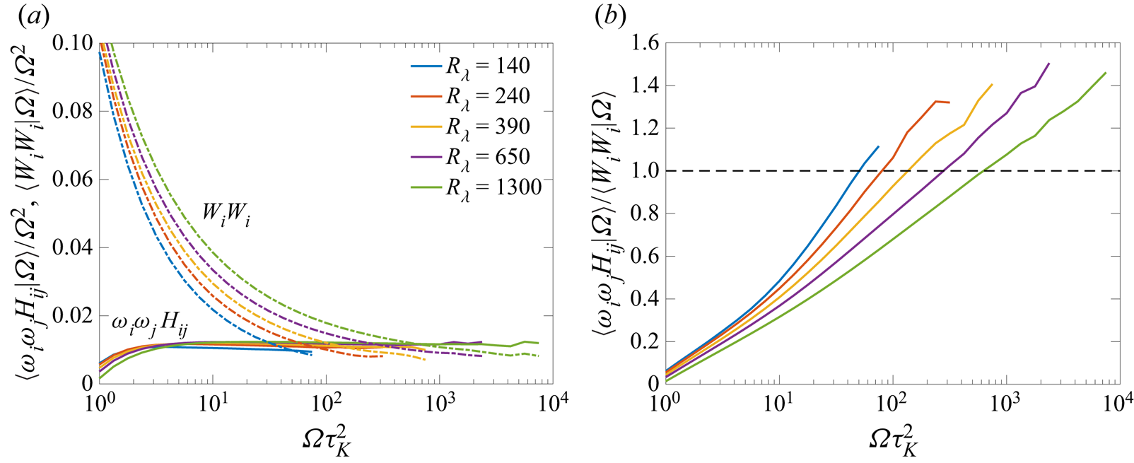
Figure 5. (a) Conditional expectations (given enstrophy  $\varOmega$) of the nonlinear and pressure Hessian contributions to the dynamics of vortex stretching vector, as given in (2.7). (a) The ratio of two terms, revealing that pressure Hessian contribution overtakes the nonlinear contribution at large
  $\varOmega$.
Further insight on the attenuation induced by the pressure Hessian in regions of intense vorticity can be obtained by rewriting (2.7) for the conditional field,
 \begin{equation} \frac{{\rm D} \langle \omega_i W_i |\varOmega \rangle }{{\rm D}t} = \langle W_i W_i | \varOmega \rangle + (-\langle \omega_i \omega_j H_{ij}^{D} |\varOmega \rangle) - (\langle \omega_i \omega_j H_{ij}^{I} |\varOmega \rangle) + \text{viscous terms} . \end{equation}
Note that the left-hand side is not zero even in stationary turbulence. We essentially observe that the first two terms on the right-hand side are positive, whereas the third term is negative, i.e. vortex stretching is enabled by the nonlinear term (which is local) and the deviatoric pressure Hessian (which is non-local), whereas the isotropic pressure Hessian (which is local) strongly opposes it. For weak or moderate  $\varOmega$, the positive contribution prevails, resulting in a net positive rate of change of vortex stretching leading to increased vorticity amplification. However, for large
  $\varOmega$, the negative contribution from
  $H_{ij}^{I}$ prevails, leading to a negative rate of change of vortex stretching. In all cases, the viscous terms are ignored, which are negligibly small at large
  ${R_\lambda }$ (although not shown, this can be anticipated).
We stress that, although the pressure Hessian is known to attenuate vortex stretching (Tsinober et al. Reference Tsinober, Ortenberg and Shtilman1999), the results in figure 5 indicate that this attenuation overwhelms even the nonlinear terms in regions of most intense vorticity. This points to an inviscid regularizing mechanism, which can be traced back to the prevalence of the contribution of  $H^I$, which can be understood as local (Ohkitani & Kishiba Reference Ohkitani and Kishiba1995). A very similar observation for attenuation of vorticity amplification was also recently uncovered in Buaria et al. (Reference Buaria, Pumir and Bodenschatz2020b) and Buaria & Pumir (Reference Buaria and Pumir2021). In these works, the non-locality of vortex stretching was analysed by writing strain as the Biot–Savart integral of vorticity and decomposing it into local and non-local contributions. The local contribution is obtained by integrating in a sphere of radius
  $R$, whereas the remaining integral is the non-local contribution. Thereafter, it was observed that vortex stretching is engendered by the non-local contribution and remarkably, the local contribution acts to attenuate intense vorticity, also representing an inviscid mechanism to counter vorticity amplification. It stands to reason that the self-attenuation mechanism identified in Buaria et al. (Reference Buaria, Pumir and Bodenschatz2020b) and Buaria & Pumir (Reference Buaria and Pumir2021) is essentially related to the local pressure mechanism identified in this work. An important underlying connection between them is that they both act only when enstrophy becomes sufficiently strong and this critical value increases with
  ${R_\lambda }$ (Buaria et al. Reference Buaria, Pumir and Bodenschatz2020b). Nevertheless, we note that precisely underpinning the causality between the two mechanisms requires further analysis, particularly by considering Lagrangian particle trajectories, as evident from (4.1). Such an analysis will be considered in a future work.
5. Role of pressure Hessian on strain amplification
While the previous section focused on the role of the pressure Hessian on vorticity amplification, we characterize here the role of the pressure Hessian on strain amplification, based on (2.6). Homogeneity implies that  $\langle S_{ij} H_{ij} \rangle = 0$, so there is no net contribution from the pressure Hessian to the budget of
  $\varSigma$. Nevertheless, the situation is quite different when isolating extreme events, with prior studies showing that pressure Hessian opposes strain amplification in regions of intense strain (Nomura & Post Reference Nomura and Post1998; Tsinober et al. Reference Tsinober, Ortenberg and Shtilman1999; Lawson & Dawson Reference Lawson and Dawson2015; Buaria et al. Reference Buaria, Pumir and Bodenschatz2022) (and thus, amplifies weak strain). In our recent work (Buaria et al. Reference Buaria, Pumir and Bodenschatz2022), we already analysed many aspects of strain amplification especially by focusing on individual eigenvalues of strain. Here, we present a complementary analysis focusing on eigenvalues of the pressure Hessian, in the spirit of the analysis in the previous section.
5.1. Unconditional statistics
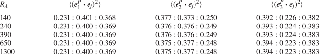
We first analyse the alignment cosines between eigenvectors of strain and the pressure Hessian, as measured by  $\langle (\boldsymbol {e}_i^{P} \boldsymbol {\cdot } \boldsymbol {e}_j)^2 \rangle$ for
  $i,j=1,2,3$. The (unconditional) average of eigenvalues of the pressure Hessian can be found in table 2, whereas those of the strain tensor were previously discussed in Buaria et al. (Reference Buaria, Bodenschatz and Pumir2020a). Table 3 lists all the nine individual terms for various
  ${R_\lambda }$, revealing no particularly strong alignment between the eigenvectors of strain and the pressure Hessian. The strongest alignment corresponds to
  $\langle (\boldsymbol {e}_1^{P} \boldsymbol {\cdot } \boldsymbol {e}_2)^2 \rangle \approx 0.4$, which is only marginally larger than
  $1/3$. Moreover, all alignment results are virtually independent of
  ${R_\lambda }$ as it was earlier the case for the alignment between vorticity and eigenvectors of pressure Hessian.
Table 3. Second moment of alignment cosines between the eigenvectors of pressure Hessian ( $\boldsymbol {e}_i^{P}$) and strain (
 $\boldsymbol {e}_j$), at various
  ${R_\lambda }$.
To rule out any anomalous behaviour, figure 6 shows the p.d.f.s of the alignment cosines. While the distributions are not exactly uniform, it can be seen that they are essentially consistent with the behaviour anticipated from their second-order moments in table 3, i.e. demonstrating some weak preferential alignment for moments larger than  $1/3$ (and vice versa). The most notable alignments are between
  $\boldsymbol {e}_2$ and
  $\boldsymbol {e}^P_1$,
  $\boldsymbol {e}^P_2$, which can be loosely understood by also considering alignment of vorticity with the eigenvectors of strain and pressure Hessian. Nevertheless, it is evident that none of the alignments are particularly strong. In all the panels, the solid and dashed lines at
  ${R_\lambda }=1300$ and
  $140$, respectively, near-perfectly coincide, showing that the alignment results are independent of
  ${R_\lambda }$.
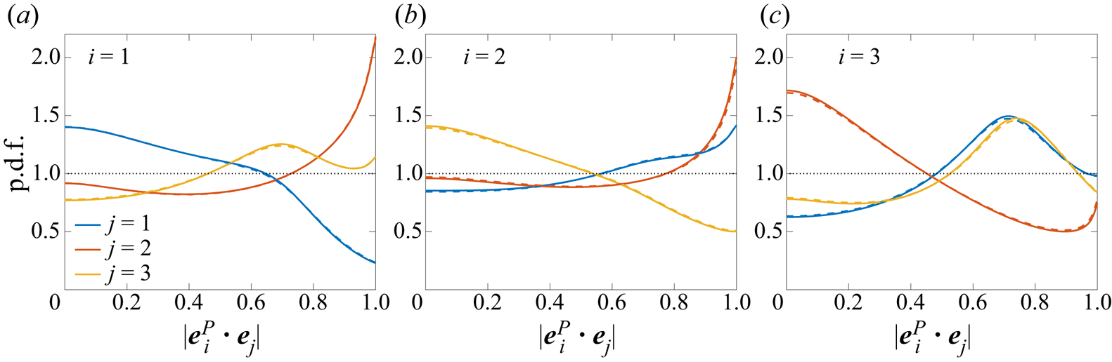
Figure 6. The p.d.f. of alignment cosines between eigenvectors of pressure Hessian ( $\boldsymbol {e}_i^{P}$) and strain (
 $\boldsymbol {e}_j$), at
  ${R_\lambda }=1300$ (solid lines) and
  ${R_\lambda }=140$ (dashed lines).
5.2. Conditional statistics
To analyse the extreme strain events, we now consider various statistics conditioned on  $\varSigma \tau _K^2$ (which equals
  $\varSigma /\langle \varSigma \rangle$). Figure 7 shows the conditional alignment between eigenvectors of strain and pressure Hessian as measured by
  $\langle (\boldsymbol {e}_i^{P} \boldsymbol {\cdot } \boldsymbol {e}_j)^2 | \varSigma \rangle$. For clarity, we only show
  ${R_\lambda }=1300$ (solid lines) and
  ${R_\lambda }=650$ (dashed lines). The dependence on
  ${R_\lambda }$ is very weak, and results at lower
  ${R_\lambda }$ (not shown) essentially follow the same trends. Overall, the alignment results indicate that there is no strong preferential alignment between strain and the pressure Hessian, even when extreme events are considered. The strongest alignments, parallel and orthogonal, are observed for
  $j=3$ and
  $j=2$, respectively, both with
  $i=3$, but the deviations from
  $1/3$ remain weak.
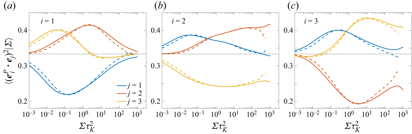
Figure 7. Conditional expectation (given  $\varSigma$) of second moment of alignment cosines between eigenvectors of pressure Hessian (
 $\boldsymbol {e}_i^{P}$) and strain (
 $\boldsymbol {e}_j$), at
  ${R_\lambda }=1300$ (solid lines) and
  ${R_\lambda }=650$ (dashed lines).
The conditional expectations of the eigenvalues of the pressure Hessian, and of its deviatoric part, are shown in figures 8(a) and 8(b), respectively. In both cases, we observe that the first and third eigenvalues are strongly positive and negative, respectively, and the second eigenvalue is very close to zero. The eigenvalues of the pressure Hessian satisfy  $\langle (\lambda _1^{P} + \lambda _2^{P} + \lambda _3^{P}) | \varSigma \rangle = \langle (\varOmega - \varSigma ) | \varSigma \rangle$. Since
  $\langle \varOmega |\varSigma \rangle \sim \varSigma$, but with a prefactor which is slightly smaller than unity (Buaria & Pumir Reference Buaria and Pumir2022; Buaria et al. Reference Buaria, Pumir and Bodenschatz2022), it follows that the sum of eigenvalues
  $\lambda _i^P$ divided by
  $\varSigma$ is a small, negative constant. Indeed, this is the observation in figure 8(a), which shows that
  $\langle -\lambda _3^{P} |\varSigma \rangle \gtrsim \langle \lambda _1^{P} |\varSigma \rangle$, whereas
  $\langle \lambda _2^{P} |\varSigma \rangle \approx 0$. On the contrary, the sum of eigenvalues of the deviatoric part is exactly zero. Indeed, figure 8(b) conforms with this expectation, with
  $\langle -\lambda _3^{D} |\varSigma \rangle \gtrsim \langle \lambda _1^{D} |\varSigma \rangle$ being still true, but
  $\langle \lambda _2^{D} |\varSigma \rangle$ is weakly positive, ensuring that the sum of the eigenvalues is zero.
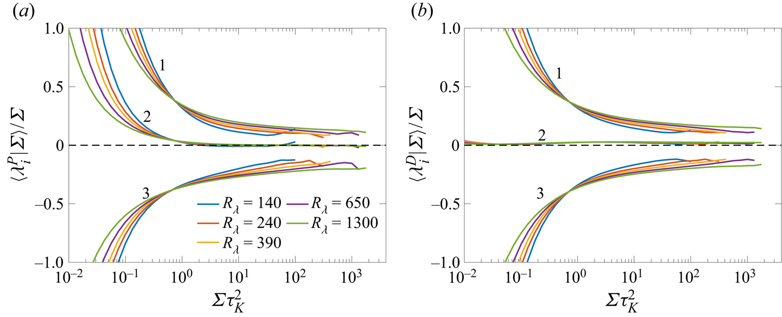
Figure 8. (a) Conditional expectation (given  $\varSigma$) of the eigenvalues of pressure Hessian, at various
  ${R_\lambda }$. (b) Conditional expectation of the eigenvalues of the deviatoric part.
Figure 9 shows the conditional expectation of the correlation  $S_{ij} H_{ij}$, together with the individual contributions from the eigendirections of pressure Hessian; figure 9(a) shows the result for pressure Hessian and its eigenvalues and figure 9(b) shows the corresponding result for the deviatoric part. Note that despite
 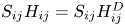 $S_{ij} H_{ij} = S_{ij} H_{ij}^{D}$, the individual contributions from their respective eigendirections differ. Given the lack of any strong alignment between strain and the pressure Hessian eigenvectors, it can be anticipated that the largest contribution to
  $S_{ij} H_{ij}$ would arise from their largest eigenvalues, i.e. the product
  $\lambda _3^{P} \lambda _3$ (or
  $\lambda _3^{D} \lambda _3$). Additionally, this contribution would be positive, since both these eigenvalues are negative. Indeed, figure 9(a,b) confirms this expectation. For both figure 9(a) and figure 9(b), the largest contribution is positive and corresponds to
  $i=3$. In contrast, the contribution for
  $i=1$ is negative, since it is dominated by the product
  $\lambda _1^{P} \lambda _3$, (or
  $\lambda _1^{D} \lambda _3$ for figure 9b). The behaviour for
  $i=2$ is not as straightforward to predict, since the alignments are non-trivial for this case. Interestingly, we observe that the contribution from
  $i=2$ is negative in figure 9(a), but weakly positive in figure 9(b). For large
  $\varSigma$, all the contributions (as divided by
  $\varSigma ^{3/2}$) appear approximately constant, implying a simple scaling (Buaria et al. Reference Buaria, Pumir and Bodenschatz2022).

Figure 9. Individual contributions to (a)  $\langle S_{ij} H_{ij} |\varSigma \rangle = \langle \lambda _i^{P} \lambda _j ( \boldsymbol {e}_i^{P} \boldsymbol {\cdot } \boldsymbol {e}_j )^2 | \varSigma \rangle$, and (b)
 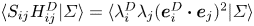 $\langle S_{ij} H_{ij}^{D} |\varSigma \rangle = \langle \lambda _i^{D} \lambda _j ( \boldsymbol {e}_i^{D} \boldsymbol {\cdot } \boldsymbol {e}_j )^2 | \varSigma \rangle$, from their eigendirections. Note, the summation is only implied over
  $j$, and results for each
  $i$ are shown. The quantities have been rescaled by
  $\varSigma ^{3/2}$. The solid lines are for
  ${R_\lambda }=1300$ and dashed lines for
  ${R_\lambda }=650$. The black lines given the total sum over all eigendirections.
The main observation from figure 9 is that the pressure Hessian term attenuates strong strain and amplifies weak strain (since the net effect has to be zero). Nevertheless, as evident from (2.6), strain amplification involves other nonlinear mechanisms. Their relative amplitudes were already compared in Buaria et al. (Reference Buaria, Pumir and Bodenschatz2022). For completeness, figure 10 shows the conditional expectations of the various inviscid terms involved in the budget equation for strain (together with their corresponding signs). All terms are once again normalized by  $\varSigma ^{3/2}$. It can be seen that the self-amplification term is the largest contribution and the primary mechanism for generating intense strain. In contrast, the vortex stretching contribution always opposes strain amplification, whereas the pressure Hessian term opposes intense strain but amplifies weak strain. When considering strong strain events (
 $\varSigma \tau _K^2 > 1$), the pressure Hessian term is noticeably weaker than vortex stretching term, and both are considerably weaker than the strain self-amplification term.
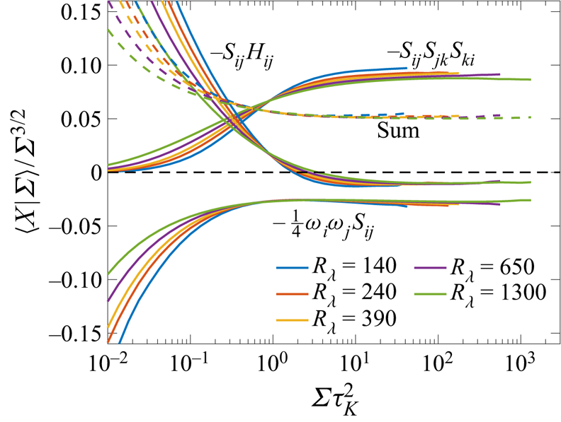
Figure 10. Conditional expectations (given  $\varSigma$) of various inviscid terms on the right-hand side of (2.6). All quantities are normalized by
  $\varSigma ^{3/2}$ revealing a plateau like behaviour for
  $\varSigma \tau _K^2 > 1$.
6. Summary and conclusions
The pressure field, via its Hessian tensor, plays a direct role in the dynamics of velocity gradient tensor  $A_{ij}$ in turbulence. Since pressure Hessian
  $H_{ij}$ is a symmetric tensor, its effect on the amplification of strain
  $S_{ij}$ (the symmetric part of
  $A_{ij}$) is explicit. However, its influence on amplification of vorticity vector
  $\omega _i$ (the skew-symmetric part of
  $A_{ij}$) comes as a second-order effect through the dynamics of the vortex stretching vector
  $W_i = \omega _j S_{ij}$. However, studies directly investigating the role of pressure Hessian on gradient amplification have been limited in the literature and when available, restricted to low Reynolds numbers. In this paper, utilizing a massive DNS database of isotropic turbulence across a wide range of Taylor-scale Reynolds numbers (
 $140 \leqslant {R_\lambda } \leqslant 1300$), we systematically investigate various statistical correlations underpinning the role of the pressure Hessian on gradient amplification and the formation of extreme events.
Overall, the pressure Hessian acts to deplete vortex stretching (and also strain amplification, which is discussed soon). Decomposing the pressure Hessian into its isotropic (local) and deviatoric (non-local) components reveals that the former opposes vortex stretching, whereas the latter favours it. There is strong cancellation between the two, such that the isotropic contribution ultimately prevails, although the net effect is significantly weaker than the nonlinear mechanism (which always enables vortex stretching). However, when the statistics are conditioned on enstrophy  $\varOmega =\omega _i \omega _i$, we find that the inhibiting effect of pressure Hessian prevails over the nonlinear mechanism, essentially leading to net depletion of vortex stretching. This depletion, which comes from the local isotropic part, suggests a natural connection to the self-attenuation mechanism recently identified in Buaria et al. (Reference Buaria, Pumir and Bodenschatz2020b) and Buaria & Pumir (Reference Buaria and Pumir2021) whereby it was shown that the self-induced local strain in regions of intense vorticity acts to attenuate further growth of vorticity. However, additional investigation is required to reinforce this connection, particularly by analysing the temporal dynamics of velocity gradients in the Lagrangian framework, which will be the subject of future work.
We further analyse the contribution of the pressure Hessian to vortex stretching in its eigenframe. For the mean field, the sum of eigenvalues is zero, resulting in the first (largest) and third (smallest) eigenvalues being nearly equal in magnitude, but opposite in sign; the second (intermediate) eigenvalue is weakly positive but essentially close to zero. No particular strong alignment is observed between vorticity and the eigenvectors of the pressure Hessian. However, when considering conditional statistics, the third eigenvalue becomes close to zero, and both the first and second eigenvalues are positive. At the same time, vorticity near perfectly aligns with the third eigenvector (while being orthogonal to other two). Structurally, this conforms with the well-known notion that intense vorticity in turbulence is arranged in tubes, which approximately correspond to the Burgers vortex. However, key differences remain, which essentially give rise to the self-attenuation mechanism, as elucidated in Buaria et al. (Reference Buaria, Pumir and Bodenschatz2020b). Considering the deviatoric and isotropic components separately allows for a simpler interpretation of how the pressure Hessian overall affects vortex stretching. Overall, not particularly strong dependence on Reynolds number is observed for all the statistics considered.
We also investigate the role of the pressure Hessian on strain amplification, which is more direct, since both tensors are symmetric. Overall, the pressure Hessian does not contribute to the budget of strain, as their correlation is zero (using homogeneity). However, when considering conditional statistics, we find that the pressure Hessian acts to oppose intense strain, but amplifies weak strain, essentially driving strain fluctuations towards the mean amplitude. Complementary to the analysis presented in Buaria et al. (Reference Buaria, Pumir and Bodenschatz2022), we focus here on the eigenframe of the pressure Hessian. As before, the first and third eigenvalues of the pressure Hessian are comparable in magnitude, but opposite in sign. This behaviour also applies when conditioning on strain magnitude. No strong alignments are observed between eigenvectors of strain and the pressure Hessian, both for unconditional and conditional fields. Because of this, the resulting behaviour strain and the pressure Hessian correlation can be deduced simply from the product of their eigenvalues. We contrast the strength of the pressure Hessian term with other nonlinear mechanisms controlling strain amplification, viz. the self-amplification term and vortex stretching. Evidently, the self-amplification term always amplifies strain; however, vortex stretching always opposes it, with its magnitude significantly weaker. The opposition from the pressure Hessian term is even weaker.
Finally, we note that many of the conditional statistics investigated here follow simple power law dependencies on vorticity or strain magnitude (when considering extreme events). We have identified these power laws in various figures as necessary. These results should prove valuable in statistical modelling of enstrophy or energy dissipation rate, particularly in p.d.f. methods (Pope Reference Pope2000). Additionally, the various conditional statistics of the pressure Hessian should also provide valuable benchmarks for Lagrangian modelling of velocity gradient dynamics (Meneveau Reference Meneveau2011). These aspects will be explored in future work.
Acknowledgements
We gratefully acknowledge the Gauss Centre for Supercomputing e.V. for providing computing time on the supercomputers JUWELS and JUQUEEN at Jülich Supercomputing Centre (JSC), where the simulations and data analyses reported in this paper were performed. A.P. acknowledges discussions with Haitao Xu and Ping-Fan Yang.
Declaration of interests
The authors report no conflict of interest.
Data availability statement
The data that support the findings of this study are available from the corresponding author upon reasonable request.
Author contributions
D.B. performed the numerical simulations and data analyses. All authors designed the research, interpreted the data and wrote the manuscript.


 Open access