


1. Introduction
Turbulent flow over rough walls has long been a subject of research as the rough walls influence the flow characteristics, such as heat and momentum transports. While turbulent flows over smooth walls are well understood, the characteristics of turbulent flows over rough walls are less predictable than those of smooth walls because the flows are subjected to properties of the roughness (Raupach, Antonia & Rajagopalan Reference Raupach, Antonia and Rajagopalan1991; Krogstad & Antonia Reference Krogstad and Antonia1994; Jiménez Reference Jiménez2004; Kadivar, Tormey & McGranaghan Reference Kadivar, Tormey and McGranaghan2021), such as the roughness packing density (i.e. closely packed or sparsely packed), roughness geometry (i.e. regular roughness such as sinusoidal, cubical and spherical or irregular/random roughness), in-plane wavelengths (i.e. varying two-dimensional or three-dimensional roughness heights) and flow types between different geometries such as pipe, closed channel and boundary layer flows. Thus, developing a universal model to predict, e.g. frictional drag on rough walls, remains challenging (Flack & Schultz Reference Flack and Schultz2010, Reference Flack and Schultz2014; Chung et al. Reference Chung, Hutchins, Schultz and Flack2021).
One of the longstanding interests in studying rough-wall-bounded turbulent flows is to assess the validity of Townsend's wall similarity hypothesis (Townsend Reference Townsend1956). The wall similarity hypothesis conjectured that the turbulence above the roughness sublayer extending to the outer region is independent of the wall surface conditions at sufficiently high Reynolds numbers. The statement equivalently states that both the turbulence intensity and the velocity defect profiles scale with friction velocity, independent of roughness and Reynolds number in the outer region, namely the outer-layer similarity (Raupach et al. Reference Raupach, Antonia and Rajagopalan1991; Jiménez Reference Jiménez2004; Flack & Schultz Reference Flack and Schultz2014; Chung et al. Reference Chung, Hutchins, Schultz and Flack2021), among others. Turbulent boundary layer (TBL) flows over regular/irregular and two/three-dimensional roughnesses were studied experimentally and numerically to explore how different types of roughness elements impact on the mean flow and turbulence quantities (e.g. Krogstad, Antonia & Browne (Reference Krogstad, Antonia and Browne1992), Krogstad & Antonia (Reference Krogstad and Antonia1994), Flack, Schultz & Shapiro (Reference Flack, Schultz and Shapiro2005), Krogstad et al. (Reference Krogstad, Andersson, Bakken and Ashrafian2005), Lee & Sung (Reference Lee and Sung2007), Volino, Schultz & Flack (Reference Volino, Schultz and Flack2011), Flack & Schultz (Reference Flack and Schultz2014), Medjnoun et al. (Reference Medjnoun, Rodriguez-Lopez, Ferreira, Griffiths, Meyers and Ganapathisubramani2021), Abdelaziz et al. (Reference Abdelaziz, Djenidi, Ghayesh and Chin2022), among others. Rough-wall TBL studies by Krogstad et al. (Reference Krogstad, Antonia and Browne1992) suggested that the mean velocity and turbulence intensity profiles were affected by the roughness well into the outer region of the TBL, as well as showing an increased fourth quadrant activity of the Reynolds shear stress near the roughness surface. It was concluded that the roughness effects were not confined to the near-wall region (Krogstad & Antonia Reference Krogstad and Antonia1994). Krogstad et al. (Reference Krogstad, Andersson, Bakken and Ashrafian2005) studied rod-roughened turbulent channel flows and showed that no influence of surface roughness in the outer region was observed in the first-order mean flow statistics, but evidence of outer flow dissimilarity was observed from the second-order statistics and in terms of the turbulence structures.
Recent studies on rough-wall flows have yielded different conclusions because the outer-layer similarity depends on a great variety of factors, such as the roughness topology, type of flow and roughness length scales (for a comprehensive discussion, see the recent review (Chung et al. Reference Chung, Hutchins, Schultz and Flack2021)). There are fundamental differences between TBL flows over two-dimensional roughness and three-dimensional roughness, e.g. Flack et al. (Reference Flack, Schultz and Shapiro2005), Schultz & Flack (Reference Schultz and Flack2005), Volino, Schultz & Flack (Reference Volino, Schultz and Flack2009), Wu & Christensen (Reference Wu and Christensen2010), Volino et al. (Reference Volino, Schultz and Flack2011), Lee, Sung & Krogstad (Reference Lee, Sung and Krogstad2011), Krogstad & Efros (Reference Krogstad and Efros2012a), Flack & Schultz (Reference Flack and Schultz2014), Yang et al. (Reference Yang, Sadique, Mittal and Meneveau2016), among others. Volino et al. (Reference Volino, Schultz and Flack2009) studied the outer-layer structure of a TBL over two-dimensional roughness and found that the two-dimensional roughness enhanced the flow motions associated with the roughness length scale, resulting in outer-layer modifications of the Reynolds stresses. Lee & Sung (Reference Lee and Sung2007) performed direct numerical simulation (DNS) studies of TBL over two-dimensional surface roughness and reported dissimilarities of the Reynolds stresses in the outer region between rough-wall and smooth-wall flows. Subsequently, Lee et al. (Reference Lee, Sung and Krogstad2011) conducted DNS of a TBL over a cube-roughened wall with three-dimensional disturbances. They found that two-dimensional and three-dimensional surface elements affect the Reynolds stress distributions in the outer layer. Flack et al. (Reference Flack, Schultz and Shapiro2005) and Schultz & Flack (Reference Schultz and Flack2005) studied the TBLs over three-dimensional regular and irregular rough surfaces and found that the first-, second- and higher-order turbulent statistics outside the roughness sublayer were independent of the wall conditions. The wall independence was confirmed by quadrant analysis of the Reynolds shear stress, which indicated that the differences in the rough-wall boundary layers were confined to the near-wall region (with distance of the order of the equivalent sand roughness height). There is a suggestion that sufficient scale separation is necessary between the roughness length scale and the outer length scale of the flow, i.e. the boundary layer thickness is large compared with the equivalent sand roughness height  $\delta /k_s\geq 40$ or equivalently, between boundary layer thickness and roughness height $\delta /k$ (Jiménez Reference Jiménez2004). However, it has been shown that the criterion using sand roughness height depends on the roughness type and is not universally applicable. The outer-layer similarity may not solely depend on $\delta /k_s$ or $\delta /k$ but also depends on the roughness morphology (Placidi & Ganapathisubramani Reference Placidi and Ganapathisubramani2018; Womack et al. Reference Womack, Volino, Meneveau and Schultz2022). Volino et al. (Reference Volino, Schultz and Flack2011) studied two-dimensional bars and three-dimensional cubes in TBLs. The authors found that two-dimensional bars with a much smaller roughness height, or $k_s/\delta$, cause a much more significant effect on turbulent structures than the three-dimensional cubes in the outer part of the boundary layer. Yang et al. (Reference Yang, Sadique, Mittal and Meneveau2016) showed that two-dimensional roughness generally has relatively stronger sheltering effects than three-dimensional roughness, due to a smaller roughness height-to-width ratio. Krogstad & Efros (Reference Krogstad and Efros2012a) suggested that for transverse bar roughness, relatively high $\delta /k$ and Reynolds number are required for outer-layer similarity to hold.
It is still a question whether or not TBLs over three-dimensional sinusoidal roughness will follow a similar trend to the previous pipes and channels studies, in which evidence of the outer-layer similarity in internal flows for certain  $k_s^+$ thresholds was observed (Chan et al. Reference Chan, Macdonald, Chung, Hutchins and Ooi2015; Ma et al. Reference Ma, Xu, Sung and Huang2020). For example, there have been studies showing that TBL over cube roughness, in which the wall-similarity could not be observed, which was viewed as the fundamental difference between external and internal flows (TBL, pipe and channel flows) (Lee et al. Reference Lee, Sung and Krogstad2011). The diagnostic plot reveals a linear asymptote between the mean flow and turbulent fluctuation, in the region extending from the logarithmic region to the outer wake region of zero-pressure-gradient (ZPG) TBLs (Alfredsson, Segalini & Örlü Reference Alfredsson, Segalini and Örlü2011; Castro, Segalini & Alfredsson Reference Castro, Segalini and Alfredsson2013), independent of whether the surface condition is smooth or fully rough. However, it can be observed that the universal scaling does not seem to apply across different flow types, such as when comparing the results of rough-wall ZPG TBLs with the channel studies (Forooghi et al. Reference Forooghi, Stroh, Schlatter and Frohnapfel2018; Stroh et al. Reference Stroh, Schäfer, Frohnapfel and Forooghi2020). In addition, it is worth noting that some of the observed roughness effects exhibit dependencies on Reynolds numbers. The roughness effects may undergo significant changes with increased friction Reynolds number and $k^+$, leading to an increasing roughness function (Busse, Thakkar & Sandham Reference Busse, Thakkar and Sandham2017).
Nevertheless, there is much literature on numerical studies of turbulent pipe and channel flows over three-dimensional regular closely packed roughness, e.g. DNS of cube arrays in channel flows (Leonardi & Castro Reference Leonardi and Castro2010; Xu et al. Reference Xu, Altland, Yang and Kunz2021), DNS of open channel flows over spherical shaped elements (Chan-Braun, García-Villalba & Uhlmann Reference Chan-Braun, García-Villalba and Uhlmann2011), three-dimensional sinusoidal roughness in DNS of pipe flows (Chan et al. Reference Chan, Macdonald, Chung, Hutchins and Ooi2015) and in DNS of channel flows (Macdonald et al. Reference Macdonald, Chan, Chung, Hutchins and Ooi2016; Ma et al. Reference Ma, Xu, Sung and Huang2020). Also, the examples of simulations of TBLs with three-dimensional regular roughness most commonly found in the literature are studies of cubical roughness in TBLs (e.g. Lee et al. Reference Lee, Sung and Krogstad2011, Reference Lee, Seena, Lee and Sung2012; Nadeem et al. Reference Nadeem, Lee, Lee and Sung2015; Blackman & Perret Reference Blackman and Perret2016; Yang et al. Reference Yang, Sadique, Mittal and Meneveau2016; Hwang & Lee Reference Hwang and Lee2018; Yang et al. Reference Yang, Xu, Huang and Ge2019). In comparison, there have been relatively limited investigations of spatially developing TBLs over three-dimensional sinusoidal roughnesses. One of the aims of the present study is to investigate the three-dimensional sinusoidal rough wall in TBLs at a higher Reynolds number range than previous studies to examine the outer-layer similarity and provide a new data set for TBLs with three-dimensional sinusoidal roughnesses.
The range of Reynolds numbers considered in the present study is determined by the simulation of spatially developing TBL that require a sufficiently long streamwise domain extent for the smooth-wall inflow to develop a fully rough-wall flow state. The present study also attempts to provide an in-depth analysis of Reynolds stress and dispersive stress transports. The Reynolds stress and dispersive stress transports arise because of the strong spatial inhomogeneities with rough-wall flows. This paper attempts to gain better insight into the development of two types of kinetic energy transports during TKE and dispersive kinetic energy generation and provides a relatively more straightforward but valuable model for studying kinetic energy balance in rough-wall flows.
Although the Reynolds and dispersive stresses for regular and irregular roughness surfaces were intensively studied by, for example, Poggi, Katul & Albertson (Reference Poggi, Katul and Albertson2004), Coceal et al. (Reference Coceal, Thomas, Castro and Belcher2006), Coceal, Thomas & Belcher (Reference Coceal, Thomas and Belcher2007b), Bailey & Smits (Reference Bailey and Smits2010), Anderson et al. (Reference Anderson, Barros, Christensen and Awasthi2015), Vanderwel et al. (Reference Vanderwel, Stroh, Kriegseis, Frohnapfel and Ganapathisubramani2019), Ma, Alamé & Mahesh (Reference Ma, Alamé and Mahesh2021), Womack et al. (Reference Womack, Volino, Meneveau and Schultz2022) and many others, there remains a need for more in-depth analysis and a demand for simple and convenient methods to investigate the distributions of Reynolds and dispersive stresses. Recently, Vanderwel et al. (Reference Vanderwel, Stroh, Kriegseis, Frohnapfel and Ganapathisubramani2019) studied a TBL over ridge-type roughness and found that the dispersive stress was not only present in the vicinity of the surface roughness but also strongly augments the Reynolds stress in the outer region:  $y/\delta > 0.1$. Vanderwel et al. (Reference Vanderwel, Stroh, Kriegseis, Frohnapfel and Ganapathisubramani2019) demonstrated that the formation of the large-scale secondary motions may play an essential role in the outer-layer distribution of the dispersive stress for both regular and irregular roughness flows. On the other hand, Ma et al. (Reference Ma, Alamé and Mahesh2021) conducted DNS of turbulent channel flow over random rough surfaces and found that the dispersive stresses are mostly confined to the roughness sublayer. The distribution of the dispersive stress varies with different types of roughness and flow geometry. Different types and arrangements of roughness exhibit distinct characteristics of the secondary flow, which in turn influence the distribution of dispersive stress (Stroh et al. Reference Stroh, Schäfer, Frohnapfel and Forooghi2020; Womack et al. Reference Womack, Volino, Meneveau and Schultz2022). The Reynolds and dispersive energy transport equations are valuable tools for the detailed analysis of the energy processes associated with turbulent and dispersive stress distribution. The second aim of this study is to present an analysis of these energy components, exploring their transport mechanisms and respective contributions to the overall energy distribution.
2. Methodology
2.1. Numerical method
An incompressible ZPG TBL over a three-dimensional sinusoidal rough wall has been considered. The streamwise, wall-normal and spanwise coordinates are denoted interchangeably as  $\boldsymbol {x} = (x,y,z)$ or $x_i$ ( $i=1,2,3$). The corresponding instantaneous velocity components are denoted interchangeably as $\boldsymbol {{u}} = ({u},{v},{w})$ or ${u}_i$. Time-averaged quantities are denoted by an overbar $(\bar {{\cdot }})$ and their fluctuation based on the Reynolds decomposition is denoted by a prime $(')$. The superscript $+$ refers to scaling with the friction velocity $u_\tau = \sqrt {\tau _w/\rho }$ and kinematic viscosity $\nu$, where $\tau _w$ is the mean wall shear stress and $\rho$ is the constant fluid density. The incompressible Navier–Stokes equations are solved using the spectral solver SIMSON (Chevalier, Lundbladh & Henningson Reference Chevalier, Lundbladh and Henningson2007). The computational domains in the streamwise, wall-normal and spanwise directions are, respectively, $L_x \times L_y \times L_z = 8000 \delta _0^* \times 200 \delta _0^* \times 240 \delta _0^*$ using $8192 \times 641 \times 768$ spectral modes, where $\delta _0^*$ is the displacement thickness at the inlet of the domain.
Spatial discretisation is based on a Fourier series with 3/2 zero-padding for dealiasing in the streamwise and spanwise directions, and the number of grid points in the streamwise and spanwise direction is therefore increased by a factor of 3/2 due to the dealiasing. A Chebyshev polynomial is employed in the wall-normal direction. To impose a streamwise periodic boundary condition, a fringe region is employed close to the end of the computational domain. The flow is damped via a volume force in the fringe region until it returns to the inflow condition (Schlatter & Örlü Reference Schlatter and Örlü2010). A low-amplitude volume force trip is applied to the Navier–Stokes equations at the region close to the inlet to trigger a rapid transition to turbulent flow (Schlatter & Örlü Reference Schlatter and Örlü2012). The time advancement is carried out by a second-order Crank–Nicolson scheme for the viscous terms and a third-order four-stage Runge–Kutta scheme for the nonlinear terms (Chevalier et al. Reference Chevalier, Lundbladh and Henningson2007).
2.2. Roughness implementation and description
In this study, the rough wall is a three-dimensional surface defined as
 \begin{equation} {h_k}(x,z) = h_0 + h_0 \cos\left( \frac{2 {\rm \pi}x}{\varOmega_x} \right)\cos\left( \frac{2 {\rm \pi}z}{\varOmega_z} \right). \end{equation}
 Figure 1 shows a schematic diagram of the rough wall. Here,  $\varOmega _x$ and $\varOmega _z$ are the streamwise and spanwise roughness wavelengths, which are fixed constants. We let $\varOmega _x = \varOmega _z = \varOmega$ so that the roughness is regular. Here $h_0$ is the roughness half-height, i.e. half of the peak to trough roughness height. From (2.1), we define the roughness height as the semiamplitude, i.e. $k=h_0$. The rough wall is modelled by the immersed boundary method (IBM). The IBM constitutes an extra forcing term introduced to the Navier–Stokes equation, where no-slip and non-penetration boundary conditions are obtained on the rough wall by enforcing zero velocities at the nearest grid points. The same numerical scheme has been successfully implemented in previous studies (Chan & Chin Reference Chan and Chin2022; Chan et al. Reference Chan, Örlü, Schlatter and Chin2022). Regarding the grid resolution for the surface roughness, first, in the present simulation, all the cases are expected to be in the fully rough regime. The wall-normal grid resolution near the rough-wall region was determined such that the grid spacing is less than $\Delta y^+_{rough,max} < 3$ in wall units. There are at least 54 Chebyshev collocation points within the region $y^+ < \max (h_k^+)$. Second, the ratios of the computational grid sizes to the roughness streamwise and spanwise wavelengths are, respectively, $\Delta x \simeq \varOmega _x/30$ and $\Delta z \simeq \varOmega _z/90$. The resolutions in the streamwise, wall-normal and spanwise directions are to ensure that the simulation is sufficient to capture the full range of length scales, including for both TBL and rough walls, as discussed by previous studies regarding grid resolution requirements for rough-wall simulations (Coceal et al. Reference Coceal, Thomas, Castro and Belcher2006; Busse, Lützner & Sandham Reference Busse, Lützner and Sandham2015). As suggested by Busse et al. (Reference Busse, Lützner and Sandham2015) for most irregular rough surfaces, $\varOmega _{min}>12$ grid points per smallest wavelength of the surface give good resolutions of the surface topographies. It is expected that this can be applied to regular rough surfaces with a relatively larger and constant wavelength. The resolution of the present simulation is listed in table 1. Cases rDNS1, rDNS2 and rDNS3 are obtained from the same DNS and correspond to different Reynolds numbers. It is important to note that the sinusoidal roughness used in these cases is identical (i.e. with constant $k/\delta _0^\ast$), see also table 2. The data set for the smooth-wall reference case, sDNS, is from Chan, Schlatter & Chin (Reference Chan, Schlatter and Chin2021). Regarding the grid resolution for the DNS of TBL, the Kolmogorov length scale $\eta \equiv (\nu ^3/\epsilon )^{1/4}$ or $\eta ^+ \equiv (\epsilon ^+)^{-1/4}$ is computed based on the local average rate of energy dissipation per unit mass, i.e. $\epsilon = 2\nu \overline {\langle {s_{ij}s_{ij}}\rangle }$ where $s_{ij}$ is the fluctuating rate of the strain tensor (Pope Reference Pope2000). From table 3, the grid resolutions are of the order of $\eta$ (i.e. $\Delta y^+ < 10\eta ^+$). Also, the computational time step $\Delta t^+$ is shown to be much lower than the Kolmogorov time scale, which is defined as $t_\eta \equiv (\nu /\epsilon )^{1/2}$ or $t_\eta ^+ \equiv (\epsilon ^+)^{-1/2}$. Overall, the numerical set-up, including the domain size and grid resolution, are comparable with those employed in previous studies on rough-wall DNS of TBL (Lee et al. Reference Lee, Sung and Krogstad2011; Cardillo et al. Reference Cardillo, Chen, Araya, Newman, Jansen and Castillo2013; Nadeem et al. Reference Nadeem, Lee, Lee and Sung2015). The computed Kolmogorov length and time scales in the present simulation suggest that the simulation is well resolved (Moin & Mahesh Reference Moin and Mahesh1998; Choi & Moin Reference Choi and Moin1994). Figure 2 shows the instantaneous streamwise velocity, mean streamwise velocity and mean streamwise vorticity contours, confirming that the rough-wall implementation is satisfactory. The present DNS was run for at least $\Delta T u_\tau ^2/\nu \approx 14\,600$ before statistics were collected. Statistics were taken and averaged for at least $\Delta T u_\tau ^2/\nu \approx 8800$.

Figure 1. Schematic of the roughness geometry. Here,  $\varOmega _x$ and $\varOmega _z$ are the streamwise and spanwise roughness wavelengths; $h_0$ is the roughness half-height (i.e. half of the peak to trough roughness height).
Table 1. Computation domain sizes and resolutions for smooth- and rough-wall cases. The reference smooth-wall case sDNS is from Chan et al. (Reference Chan, Schlatter and Chin2021). Here,  $N_x$, $N_y$ and $N_z$ are the numbers of spectral collocation points in the streamwise, wall-normal and spanwise directions, respectively; $L_x$, $L_y$ and $L_z$ are the domain sizes scaled by $\delta _0^\ast$ in the streamwise, wall-normal and spanwise directions, respectively; $\delta _0^*$ is the displacement thickness at the inlet of the domain; $\Delta x^+$, $\Delta y_{min}^+$, $\Delta y_{max}^+$ and $\Delta z^+$ are the corresponding grid resolutions in wall units.

Table 2. Reynolds numbers and rough-wall parameters of smooth-wall and rough-wall cases. Here  $Re_\tau \equiv \delta ^+$, where $\delta$ is the boundary layer thickness; $Re_\theta \equiv U_\infty \theta /\nu$, where $\theta$ is the momentum thickness; $h_{rms}^+$ is the root-mean-square roughness height (2.2); $ES$ is the effective slope (2.4); $h_a$ is the mean roughness height (2.3); $k^+$ is the roughness height defined as the semiamplitude; $\varOmega$ is the roughness wavelength; $u_\tau /U_\infty$ is the friction velocity; and $e$ is the wall offset.
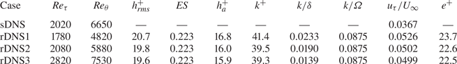
Table 3. Grid resolutions for the rough-wall TBL. Here,  $\epsilon ^+ \equiv 2\nu \overline {\langle {s_{ij}s_{ij}}\rangle }^+$ where $s_{ij}$ is the fluctuating rate of the strain tensor (Pope Reference Pope2000). For the TKE transport, we denote $\epsilon ''^+_K = (1/2)\epsilon ^+$. Here, $\eta ^+ \equiv (\epsilon ^+)^{-1/4}$ is the Kolmogorov length scale, and $t_\eta ^+ \equiv (\epsilon ^+)^{-1/2}$ is the Kolmogorov time scale.


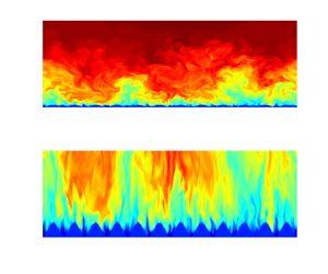
Figure 2. Realisations of rough-wall TBL. (a) Instantaneous streamwise velocity contour  $u/U_\infty$ (normalised by the free stream velocity $U_\infty$) at $Re_\tau = 2820$ ( $x/\delta _0^\ast =6500$). (b,c) Time-averaged streamwise velocity contour (and isolines) $\bar {u}/U_\infty$ and time-averaged streamwise vorticity contour $\bar {\omega }_x^+$ at $Re_\tau = 2820$ ( $x/\delta _0^\ast =6500$). High-momentum paths (HMP) and low-momentum paths (LMP) are indicated by dashed and solid lines, respectively. (d) Instantaneous streamwise velocity $u/U_\infty$ (flow from left to right) at $x/\delta _0^\ast = 2780-3075$ ( $Re_\tau \approx 1700$), $z/\delta _0^\ast = 130$.
Parameters that characterise the roughness surface are listed in table 2. The global averaged boundary layer parameters variations in the streamwise direction, including the (a) boundary layer thickness, (b) displacement thickness, (c) momentum thickness and (d) shape factor, are presented in figure 3. Compared with the smooth-wall TBL, the rough-wall TBL exhibits higher boundary layer parameters at the same streamwise distance. An important parameter to compare is the shape factor  $H$, defined as the ratio of displacement to momentum thickness, characterising the development state of a boundary layer. The shape factor converges at approximately $x/\delta _0^\ast \geq 2500$ or equivalently at approximately $Re_\tau \geq 1700$, indicating a fully developed turbulent state. The root-mean-square roughness height is defined as
 \begin{equation} h^2_{rms} = \frac{1}{A_{xz}}\iint\left(h_k(x,z)-h_m\right)^2\,\mathrm{d}\,x\, \mathrm{d}z, \end{equation}
where  $A_{xz} = L_x L_z$ is the roughness surface area and $h_m = h_0$ is the roughness mean height. The average height of the roughness is defined as
 \begin{equation} h_a = \frac{1}{A_{xz}}\iint\left|h_k(x,z)-h_m\right|\,\mathrm{d}\,x\, \mathrm{d}z. \end{equation}
For three-dimensional sinusoidal surfaces,  $h_a$ is simply linked to the root-mean-square roughness height as $h_a = (4/{\rm \pi} ^2)h_0 = (8/{\rm \pi} ^2)h_{rms}$. The parameter that defines the steepness of the roughness topography is the effective slope. For three-dimensional roughness, the effective slope can be defined as (Napoli, Armenio & De-Marchis Reference Napoli, Armenio and De-Marchis2008; Chan et al. Reference Chan, Macdonald, Chung, Hutchins and Ooi2015; Ma et al. Reference Ma, Xu, Sung and Huang2020)
 \begin{equation} ES = \frac{1}{A_{xz}}\iint\left|{\partial_x h_k(x,z)}\right|\,\mathrm{d}\,x\, \mathrm{d}z. \end{equation}
The effective slope is used to characterise the geometry of irregular roughnesses. It is shown that the effective slope relates to the solidity parameter  $\varLambda$ such that $ES = 2\varLambda$ (Napoli et al. Reference Napoli, Armenio and De-Marchis2008). The solidity is the ratio between the total projected frontal roughness area and the wall-parallel projected area (Napoli et al. Reference Napoli, Armenio and De-Marchis2008; Macdonald et al. Reference Macdonald, Chan, Chung, Hutchins and Ooi2016; Forooghi et al. Reference Forooghi, Stroh, Magagnato, Jakirlić and Frohnapfel2017) (and for a smooth-wall $\varLambda =0$). For regular roughness, the effective slope accounts for the streamwise periodicity of the roughness pattern and the roughness height. In the present case, $ES = (8k/{\rm \pi} \varOmega )$.

Figure 3. Global averaged boundary layer parameter variations in the streamwise direction between smooth-wall and rough-wall cases: (a) boundary layer thickness  $\delta$; (b) displacement thickness $\delta ^*$; (c) momentum thickness $\theta$; and (d) shape factor $H$.
$H$.
2.3. Velocity decomposition
In addition to the velocity fluctuation obtained based on the Reynolds decomposition. The velocity fluctuation is also obtained based on the triple decomposition (also known as the double-averaging procedure) (Raupach & Shaw Reference Raupach and Shaw1982; Nikora et al. Reference Nikora, Goring, McEwan and Griffiths2001). The triple decomposition differs from the Reynolds decomposition, where the time-averaged quantity is further averaged in the spatial direction, resulting in an additional dispersive fluctuation (also known as the coherent fluctuation) representing the spatial variation of the time-averaged flow,
 $$\begin{gather} q(x,y,z,t) = \bar{q} (x,y,z) + q'(x,y,z,t), \end{gather}$$
 $$\begin{gather}q(x,y,z,t) = \langle \bar{q} \rangle (x,y) + q'(x,y,z,t) + \tilde{q}(x,y,z), \end{gather}$$
where  $q$ represents an instantaneous fluid-defined flow variable; $\bar {q}$ denotes the time-averaged value; $q'$ denotes the corresponding fluctuation (i.e. turbulent fluctuation) based on the Reynolds decomposition (2.5); and $\tilde {q}$ denotes the corresponding dispersive fluctuation. The $\langle {\cdot } \rangle$ denotes a spatial-averaging procedure,
 \begin{equation} \langle \bar{q} \rangle(x,y) = \frac{1}{L_{z,f}(x,y)}\int_{z,f}{ \bar{q}(x,y,z)} \,\mathrm{d}z, \end{equation}
where  $L_{z,f}$ is the spanwise width occupied by fluid and $0 < L_{z,f}(x,y)/L_z \leq 1$. Accordingly, the dispersive fluctuation $\tilde {q}$ represents the induced-spatial variation of the time-averaged flow due to the presence of roughness. From the triple decomposition (2.6) let $q=u_i$, the total velocity fluctuations can be defined as
 \begin{equation} {u}''_{i}(\boldsymbol{x},t) = {u}'_{i}(\boldsymbol{x},t) + \tilde{{u}}_{i}(\boldsymbol{x}), \end{equation}
where, by definition,  $\overline {u''_i} = \tilde {{u}}_{i}$, and the Reynolds (turbulent) stress tensor $\overline {{u}'_{i} {u}'_{j}}$ can be written as (e.g. Türk et al. Reference Türk, Daschiel, Stroh, Hasegawa and Frohnapfel2014; Vanderwel et al. Reference Vanderwel, Stroh, Kriegseis, Frohnapfel and Ganapathisubramani2019; Ma et al. Reference Ma, Alamé and Mahesh2021)
 \begin{equation} \overline{{u}'_{i} {u}'_{j}} (\boldsymbol{x} ) = \overline{{u}''_{i} {u}''_{j}} (\boldsymbol{x} ) - \tilde{{u}}_{i} \tilde{{u}}_{j} (\boldsymbol{x} ), \end{equation}
where, on the right-hand side of (2.9), the first term represents the total stress tensor, and the second term represents the dispersive stress tensor.
2.4. Friction velocity estimation
There are several direct and indirect methods for computing the friction velocity  $u_\tau$ values. The direct method is based on the streamwise and wall-normal components of the mean momentum equation by assuming that the boundary layer is two-dimensional. The integrated mean momentum equation can be solved numerically and is generally suitable for data collected from numerical simulations with sufficient streamwise measurements. The mean momentum integral equation reads as (Brzek et al. Reference Brzek, Cal, Johansson and Castillo2007)
 \begin{align} \tau_w(x) &= \left.\nu {\partial_y \bar{u}}\right\vert_{y_a}-\left.\overline{u'v'}\right\vert_{y_a} + \int U_\infty{\partial_x U_\infty}\,\mathrm{d} y\nonumber\\ &\quad -\int \partial_x(\overline{u'u'}) - \partial_x(\overline{v'v'}) \,\mathrm{d} y - \int {\partial_x ({\bar{u} \,\bar{u}}) } \,\mathrm{d} y - \left.\bar{u}\,\bar{v}\right\vert_{y_a}, \end{align}
for an arbitrary chosen wall-normal location  $y_a >e$. The friction velocity based on the mean wall shear stress is defined as
 \begin{equation} (u_\tau/U_\infty)^2 = (\tau_w/(\rho U_\infty^2))^2 = C_f/2. \end{equation}
A limitation of this method is that it is computationally more costly than most other methods, especially for the DNS of TBL. Apart from the direct approach, there are also several indirect approaches to compute the friction velocity. Many indirect approaches often require much fewer flow measurements, especially when the near-wall measurement is not available, and thus are commonly used for numerical and experimental data sets. The modified Clauser method computes the friction velocity by fitting the rough-wall data to an assumed log-law region of the mean velocity profile (Perry & Li Reference Perry and Li1990). A limit is that the choice of  $u_\tau$ and virtual origin of the wall might not be unique at low Reynolds numbers. Another possible method is based on the assumption of outer-layer similarity (see e.g. Monty et al. Reference Monty, Allen, Lien and Chong2011). From this approach, one first computes a pair of initial values for the friction velocity and virtual wall offset based on the modified Clauser method. Then, one assumes that the outer-layer similarity holds for the mean velocity and streamwise velocity fluctuation intensity profile under outer scaling and systematically fits the rough-wall data to the smooth-wall data and minimises the combined difference for a range of $u_\tau$. Subsequently, the assumption of outer-layer similarity is checked by plotting outer-scaled data using the assumed friction velocity and virtual wall origin. The argument implies that the outer-layer similarity hypothesis is invalid if outer-scaled data do not collapse well. Recently, Kumar & Mahesh (Reference Kumar and Mahesh2022) proposed an indirect method to determine the wall shear stress based on a mean stress model (Kumar & Mahesh Reference Kumar and Mahesh2021). This method does not require near-wall measurements and is applicable to both smooth- and rough-wall TBL. In this study, the friction velocity is computed based on the mean stress model. The friction velocity is recast as
 \begin{equation} u_\tau = \frac{1}{\zeta_1-\zeta_0}\int_{\zeta_0}^{\zeta_1} \left\langle\sqrt{\frac{{\varTheta}(\zeta)}{1-\bar{u}(\zeta)\bar{v}(\zeta)/U_eV_e}}\right\rangle \,\mathrm{d}\zeta, \end{equation}
where  $\varTheta$ is the sum of viscous stress and Reynolds shear stress, $\zeta =y_e/\delta$, $U_e = \bar {u}(y_e=\delta )$ and $V_e = \bar {v}(y_e=\delta )$, where $y_e^+ = (y^+-e^+)$, and $e$ is offset from the reference virtual plane for rough-wall TBL (table 2). In the present study, the offset is defined as the location of the zero mean streamwise velocity at the farthest point from the wall: a condition that is also satisfied by the no-slip condition at the surface of the smooth-wall case. The boundary layer thickness is thus defined as $\delta = \langle y(\bar {u}=0.99 U_\infty )-y(\bar {u} = 0) \rangle$ or $\delta = \langle y(\bar {u} = 0.99 U_\infty )-e\rangle$. In this paper $\zeta _1 = 0.35$ and $\zeta _0 = 0.2$ are used based on ideal values according to Kumar & Mahesh (Reference Kumar and Mahesh2022). We define the friction velocity based on this method as it does not require an adjustment to account for wall roughness and has been shown to be robust over a range of Reynolds numbers for both smooth- and rough-wall ZPG TBL (Kumar & Mahesh Reference Kumar and Mahesh2022). It is relatively insensitive to the choice of the virtual origin of the wall, the shape factor $H$ and the size of the data set. It is, therefore, suitable for the current data set, and a robust friction velocity value can be obtained at a reasonable computational expense.
Additional comparisons between the friction velocity  $u_{\tau,1}$ obtained based on the mean stress model (Kumar & Mahesh Reference Kumar and Mahesh2022) and the comprehensive shear stress (CSS) method (Womack, Meneveau & Schultz Reference Womack, Meneveau and Schultz2019) are presented. Unlike the mean stress model, the CSS method is an iterative method based on the rescaled mean momentum integral equation and the log-law equation. To determine the friction velocity, $u_{\tau,2}$, the total shear stress balance was first fitted in the range $0.15 < (y-e_2)/\delta < 0.3$, where $\delta = \langle y(\bar {u} = 0.99 U_\infty )-e_2\rangle$. The log-law equation was then fitted in the range $0.07 < (y-e_2)/\delta < 0.15$ to estimate the roughness length $l_{s,2}$ and the wall offset
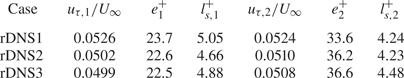
  $e_2$ (Volino & Schultz Reference Volino and Schultz2018; Womack et al. Reference Womack, Meneveau and Schultz2019, Reference Womack, Volino, Meneveau and Schultz2022). Table 4 shows the friction velocity computed based on the mean stress model and the CSS method. Overall, the mean stress model consistently yields similar results to the CSS method. It was also checked that the small discrepancy in the actual value of friction velocity does not affect the inner-scaled profiles discussed in the results section. Therefore, in the results section, the friction velocity is based on the mean stress model. The $u_\tau$ values computed based on (2.12) for the rough-wall cases are listed in table 2.
Table 4. Friction velocity estimation based on the mean stress model ( $u_{\tau,1}$) (Kumar & Mahesh Reference Kumar and Mahesh2022) and CSS method ( $u_{\tau,2}$) (Womack et al. Reference Womack, Meneveau and Schultz2019). Here, $l_{s,1}^+$ and $l_{s,2}^+$ denote the roughness length estimated based on $(u_{\tau,1}, e_1^+)$ and $(u_{\tau,2}, e_2^+)$, respectively.
3. Results and discussion
3.1. Mean velocity flow
The mean velocity profile in rough-wall flow relating to the roughness Reynolds number  $k^+$ is expected to follow the log-law profile in the form of
 \begin{equation} \langle\bar{u}\rangle^+= U^+= \frac{1}{\kappa}\ln (y_e^+) + B - \Delta U^+, \end{equation}
where the von Kármán constant is  $\kappa = 0.384$, the smooth-wall intercept is $B=4.17$ (Marusic et al. Reference Marusic, Monty, Hultmark and Smits2013; Womack et al. Reference Womack, Volino, Meneveau and Schultz2022). Here $\Delta U^+$ is the Hama roughness function that measures the downward shift in the log law region compared with the smooth-wall case (Hama Reference Hama1954). Figure 4(a) presents the inner-scaled mean velocity profiles for the rough-wall TBL and smooth-wall TBL. The mean velocity profiles of the rough-wall TBL at three different Reynolds numbers clearly present a constant downward shift in the logarithmic overlap region compared with smooth-wall TBL. The rough-wall profiles exhibit a log–linear region with a slope of approximately $1/\kappa$ between approximately $200 \leq y_e^+ \leq 400$. The roughness function $\Delta U^+$, is thus determined based on (3.1) at $y_e^+ \simeq 200-400$ with the inner-scaled profile for the smooth-wall case. This gives $\Delta U^+ \simeq 8.3$ for rough-wall cases rDNS1, rDNS2 and rDNS3, indicating that all the rough-wall cases are in the fully rough regime. The roughness function associated with the present sinusoidal roughness is greater than that observed for cube roughness (Lee et al. Reference Lee, Sung and Krogstad2011). The difference in the roughness function can be attributed to various roughness parameters, including the roughness aspect ratio, effective slope and skewness factor. Previous studies have also shown that the roughness function is indeed influenced by the $k^+$ and Reynolds number for both irregular and regular surfaces. Specifically, the roughness effects tend to increase with the friction Reynolds number and $k^+$ (Chan et al. Reference Chan, Macdonald, Chung, Hutchins and Ooi2015; Busse et al. Reference Busse, Thakkar and Sandham2017; Ma et al. Reference Ma, Xu, Sung and Huang2020). Notably, investigations conducted by Volino et al. (Reference Volino, Schultz and Flack2011) and Lee et al. (Reference Lee, Sung and Krogstad2011) on cubical roughness have provided evidence of the dependence on $k^+$ and $Re_\tau$, which is associated with an increasing roughness function. Similar observations have been made for three-dimensional sinusoidal roughness in turbulent channel flows, as demonstrated in the study by Ma et al. (Reference Ma, Xu, Sung and Huang2020). Since the present case is in the fully rough regime (Flack & Schultz Reference Flack and Schultz2010), the equivalent sand grain roughness, $k_s^+ = k_su_\tau /\nu$, is estimated based on the $\Delta U^+ - k_s^+$ relationship as
 \begin{equation} \ln k_s^+= \kappa(\Delta U^+ + 8.5-B), \end{equation}
for the collapsing of rough surfaces in the fully rough regime where  $\Delta U^+ > 7.0$ (Flack & Schultz Reference Flack and Schultz2010) and this gives $k_s^+ \simeq 128$ for all rough-wall cases. The equivalent sand grain roughness is a common roughness length scale used to compare the roughness function between different types of roughness flows with uniform sand grains by Nikuradse (Reference Nikuradse1933). In addition, we obtain the relationship $k_s^+ \simeq 3.2 k^+$ for the present sinusoidal roughness. This value is slightly smaller than those reported by Chan et al. (Reference Chan, Macdonald, Chung, Hutchins and Ooi2015) and Ma et al. (Reference Ma, Xu, Sung and Huang2020) for three-dimensional sinusoidal roughness. Figure 4(b) presents the mean velocity profile in a velocity-defect form where the flow similarity in the outer part of the boundary layer can be observed, suggesting that the direct influence of roughness is mainly confined to the roughness sublayer, $y_e^+ < y^+_r$, where the roughness sublayer is typically assumed to have a wall-normal extent of five times of the roughness height or $y^+_r \leq 5(k^+)$ (Jiménez Reference Jiménez2004; Lee et al. Reference Lee, Sung and Krogstad2011; Chung et al. Reference Chung, Hutchins, Schultz and Flack2021). The flow similarity manifests as outer-layer or wall similarity (Townsend Reference Townsend1956), which states that in the outer region of the flow, regardless of smooth or rough surface conditions, the turbulent motion is independent of the surface condition and that implies mean flow and turbulent statistics agree well between smooth- and rough-wall cases in the outer region of the flow (Raupach et al. Reference Raupach, Antonia and Rajagopalan1991; Chung et al. Reference Chung, Hutchins, Schultz and Flack2021; Kadivar et al. Reference Kadivar, Tormey and McGranaghan2021). The mean defect velocity profiles in TBLs over various roughness types are plotted in figure 4(b) for comparison. The mean defect velocity profiles also exhibit similarity in the outer region when compared with profiles obtained for staggered cubes, transverse rods and bars. The equivalent sand grain roughness $k_s^+$ ranges from the transitionally rough regime, $k_s^+ = 57.9$ for staggered cubes (Lee et al. Reference Lee, Sung and Krogstad2011) to the fully rough regime, $k_s^+ = 755$ for large bars (Volino et al. Reference Volino, Schultz and Flack2011). This similarity suggests that the mean flow may be minimally affected by the differences in roughness types between sinusoidal and cubical rough surfaces.

Figure 4. (a) Mean streamwise velocity profile and (b) mean velocity defect profile. Coloured symbols are rDNS1 (red  $\triangle$), rDNS2 (blue $\circ$), rDNS3 (green $\square$). Solid black line is sDNS. The dashed lines for the sDNS case denote linear $\langle \bar {u} \rangle ^+ = y^+$ and log-law region $\langle \bar {u} \rangle ^+ = 1/\kappa \log y^+ + C$ with $\kappa = 0.384$, $C=4.17$. $(c,d)$ Profiles of Reynolds shear stress $\langle \overline {-u'v'} \rangle ^+$ and dispersive shear stress $\langle {-\tilde {u}\tilde {v}} \rangle ^+$ in (c) inner and (d) outer coordinates. Dashed lines denote the dispersive shear stress for rDNS1 (red), rDNS2 (blue), rDNS3 (green). The vertical dashed line in (c) denotes the maximum height of the roughness, $k_e^+ = 2k^+-e^+$ for the case rDNS1 with magnitude similar to that of rDNS2 and rDNS3. Black symbols in (b,d) are ( $\triangle$) small square transverse bars, ( $\bullet$) staggered cubes and ( ${_{_\bigtriangledown}}$) large square transverse bars (Volino et al. Reference Volino, Schultz and Flack2011); ( $\circ$) transverse rods and ( $\square$) staggered cubes (Lee, Sung & Krogstad Reference Lee, Sung and Krogstad2011).
3.2. Reynolds and dispersive stresses
Figure 4(c,d) shows profiles of the Reynolds shear stress and dispersive shear stress obtained by (2.9) and plotted in inner and outer coordinates. Figure 4(c) shows that for the Reynolds shear stress, the Reynolds number effect (the Reynolds number increases in the arrow direction) is seen in the outer region  $y_e^+ > 10^3$, and the case rDNS2 ( $Re_\tau =2080$) collapses well to the sDNS ( $Re_\tau =2020$) because of the similar Reynolds numbers. The Reynolds number effect is small when plotting the Reynolds shear stress in outer coordinates, as shown in figure 4(d). The Reynolds shear stress profile is further compared across the present roughness type and various other roughness types in figure 4(d). The evidence of outer-layer similarity is less pronounced in the Reynolds shear stress profile, particularly when comparing the large square transverse bars with the other cases. This observation aligns with the findings of Volino et al. (Reference Volino, Schultz and Flack2011), who noted that the outer-layer effects appear to be more prominent in the Reynolds shear stress profile of rough-wall TBLs. The difference in the outer layer may be attributed to the roughness dimensions rather than solely being a result of variations in $k^+$ or $k/\delta$ values. Compared with the Reynolds shear stress, the dispersive shear stress is mainly confined to the roughness sublayer. This is consistent with the observations of Poggi et al. (Reference Poggi, Katul and Albertson2004), Coceal et al. (Reference Coceal, Thomas, Castro and Belcher2006), Coceal et al. (Reference Coceal, Thomas and Belcher2007b) and Bailey & Stoll (Reference Bailey and Stoll2013) for flow over regular plant canopies and is similar to the observation of Ma et al. (Reference Ma, Alamé and Mahesh2021) for random rough surfaces. The Reynolds normal stress components are plotted in figure 5.

Figure 5. Reynolds and dispersive stress profiles. Legend as per figure 4.
For figure 5(a–c), the near-wall peak of the streamwise Reynolds stress, which is observed in the smooth-wall case, is not observed in the rough-wall cases, while the wall-normal and spanwise Reynolds stress components increase in magnitude at  $100 \leq y_e^+ \leq 500$ for all cases. The increase in magnitude for the spanwise component is more pronounced than that of the wall-normal component. Overall, the variation in the streamwise turbulence intensity and the increases in the wall-normal and spanwise turbulence intensities at a matched Reynolds number are consistent with the observations by Krogstad & Antonia (Reference Krogstad and Antonia1999) and Chan et al. (Reference Chan, Macdonald, Chung, Hutchins and Ooi2015). For all Reynolds normal stress components, the rDNS2 case collapses to the sDNS case in the outer region, as the Reynolds numbers for both cases are similar. Therefore, the slight discrepancies for all three Reynolds stress components between the smooth-wall case, and the rough-wall cases rDNS1 and rDNS3, are due to the Reynolds number effect. Additionally, the dispersive normal stresses and dispersive shear stress are primarily confined to the roughness sublayer, suggesting that the secondary motion is confined within the roughness layer. For figure 5(d–f), similarity in the variance in the outer region between the smooth-wall case and the present rough-wall cases is observed. Interestingly, for the rough-wall cases, small $Re_\tau$ dependence may be observed, as indicated by the arrow. However, this is not observed for rough-pipe flows (Chan et al. Reference Chan, Macdonald, Chung, Hutchins and Ooi2015). The streamwise Reynolds stress profiles between the present and various previous roughness types are compared again in figure 5(d). A similarity is observed between most of the profiles in the outer region $y_e > 0.8 \delta$ for different roughness geometries. However, for $y_e < 0.8 \delta$, a noticeable deviation of the inner-scaled streamwise Reynolds stress is evident, and strongly depends on the specific roughness type.
3.3. Linear asymptote in the diagnostic plot
Outer-layer behaviour in the streamwise mean velocity and root-mean-square turbulent fluctuation is further examined through the diagnostic plot (Alfredsson et al. Reference Alfredsson, Segalini and Örlü2011, Reference Alfredsson, Örlü and Segalini2012; Alfredsson, Segalini & Örlü Reference Alfredsson, Segalini and Örlü2021). The diagnostic plot reveals that, at least in the case of smooth-wall ZPG TBLs, within the flow region extending from the logarithmic region and reaching almost the entire outer wake region, a linear asymptote exists between streamwise mean velocity and root-mean-square turbulent fluctuation, characterised by  ${\langle \overline {u'u'}\rangle }^{1/2}/\langle \bar {u} \rangle = a - b \langle \bar {u} \rangle /U_\infty$, where $a$ and $b$ are constants obtained from smooth-wall data.
Castro et al. (Reference Castro, Segalini and Alfredsson2013) further showed that in the case of transitional and fully rough ZPG TBLs, the rough-wall linear asymptote may also be expressed by  ${\langle \overline {u'u'}\rangle }^{1/2}/\langle \bar {u} \rangle = \hat {a}-\hat {b} \langle \bar {{u}} \rangle /U_\infty$. Subsequently, Castro et al. (Reference Castro, Segalini and Alfredsson2013) proposed a modified form of the rough-wall linear asymptote, i.e. ${\langle \overline {u'u'}\rangle }^{1/2}/\langle (\bar {u}+\Delta U) \rangle = \hat {a}-\hat {b} \langle (\bar {u}+\Delta U) \rangle /(U_\infty +\Delta U)$. In this modified form where $\Delta U$ is the roughness function, and $\tilde {a} \simeq a$, $\tilde {b} \simeq b$. This suggests a universal scaling between the streamwise mean velocity and root-mean-square turbulent fluctuation, applicable to both smooth-wall and rough-wall ZPG TBLs (at least in fully rough conditions). This universality appears to be independent of the friction velocity value and the choice of wall offset (Castro et al. Reference Castro, Segalini and Alfredsson2013).
Figure 6(a) displays the diagnostic plot for data sets of smooth-wall and rough-wall TBLs, including the present sinusoidal roughness cases and data sets from prior studies on rough-wall TBLs.

Figure 6. (a) Diagnostic plot of the mean streamwise velocity and root-mean-square turbulent fluctuation (Alfredsson et al. Reference Alfredsson, Segalini and Örlü2011; Alfredsson, Örlü & Segalini Reference Alfredsson, Örlü and Segalini2012) and (b) modified empirical scaling form (Castro et al. Reference Castro, Segalini and Alfredsson2013). Solid black line: sDNS. Coloured symbols are rDNS1 (red  $\triangle$), rDNS2 (blue $\circ$) and rDNS3 (green $\square$). The red dashed line denotes linear smooth-wall asymptote, ${\langle \overline {u'u'}\rangle }^{1/2}/\langle \overline {u} \rangle = a - b \langle \overline {u} \rangle /U_\infty$, where ${a = 0.25}, {b = 0.21}$. The black dashed line denotes linear rough-wall asymptote, ${\langle \overline {u'u'}\rangle }^{1/2}/\langle \overline {u} \rangle = \hat {a}-\hat {b} \langle \overline {{u}} \rangle /U_\infty$, where ${\hat{a} = 0.34}, {\hat{b} = 0.29}$. Black symbols in (a,b) are ( $\circ$) (Flack, Schultz & Connelly Reference Flack, Schultz and Connelly2007), ( $\square$) (Krogstad & Efros Reference Krogstad and Efros2012), ( $\ast$) (Brzek et al. Reference Brzek, Cal, Johansson and Castillo2008), ( $\diamond$) (Medjnoun et al. Reference Medjnoun, Rodriguez-Lopez, Ferreira, Griffiths, Meyers and Ganapathisubramani2021), ( $+$) (Amir & Castro Reference Amir and Castro2011) and (— - — -) (Forooghi et al. Reference Forooghi, Stroh, Schlatter and Frohnapfel2018).
It can be observed that both smooth-wall and rough-wall TBLs exhibit distinct linear asymptotes. The present sinusoidal roughness cases and other rough-wall cases collapse to a rough-wall linear asymptote with  $\hat {a} = 0.34$ and $\hat {b} = 0.29$ (Flack et al. Reference Flack, Schultz and Connelly2007; Brzek et al. Reference Brzek, Cal, Johansson and Castillo2008; Amir & Castro Reference Amir and Castro2011; Krogstad & Efros Reference Krogstad and Efros2012; Castro et al. Reference Castro, Segalini and Alfredsson2013), and the smooth-wall TBL data set aligns with a smooth-wall linear asymptote characterised by ${a} = 0.25$ and ${b} = 0.21$.
This lack of collapse between the smooth-wall and rough-wall cases is attributed to the increase in streamwise turbulent intensity, primarily due to the non-zero roughness function  $\Delta U$ observed in the rough-wall cases. This finding aligns well with the observations made by Castro et al. (Reference Castro, Segalini and Alfredsson2013) and is confirmed in figure 6(b). In figure 6(b), the modified form of the diagnostic plot is presented. The inclusion of the roughness function in the modified scaling reveals a remarkable collapse starting at $(\langle \bar {u} \rangle +\Delta U)/({U}_\infty +\Delta U) \simeq 0.4$. This collapse is observed among the present sinusoidal roughness cases, previous roughness cases and the smooth-wall case (Flack et al. Reference Flack, Schultz and Connelly2007; Brzek et al. Reference Brzek, Cal, Johansson and Castillo2008; Amir & Castro Reference Amir and Castro2011; Krogstad & Efros Reference Krogstad and Efros2012; Castro et al. Reference Castro, Segalini and Alfredsson2013). A similar argument also holds for root-mean-square total fluctuation, as demonstrated by Medjnoun et al. (Reference Medjnoun, Rodriguez-Lopez, Ferreira, Griffiths, Meyers and Ganapathisubramani2021), and is depicted in figure 6.
We have also observed that the universal scaling does not apply when comparing flow data sets of different flow types. The discrepancy is illustrated by including a turbulent channel case studied by Forooghi et al. (Reference Forooghi, Stroh, Schlatter and Frohnapfel2018). There is no collapse observed between all the rough-wall ZPG TBL cases and the turbulent channel case. Notably, prior findings reported had consistently identified universal behaviour within channel results (Forooghi et al. Reference Forooghi, Stroh, Schlatter and Frohnapfel2018; Stroh et al. Reference Stroh, Schäfer, Frohnapfel and Forooghi2020).
The analysis provides partial evidence of the universal outer-layer behaviour in the diagnostic plot between smooth-wall and rough-wall TBLs when modified to account for the  $\Delta U$. Consequently, $\Delta U$ appears to play a significant role in generating the linear collapse in the outer region between smooth-wall and rough-wall TBLs despite the different roughness morphologies and turbulence structures in the outer region of smooth-wall and rough-wall TBLs.
3.4. Spanwise length scales and mean structure angles
A comparison of turbulent structures over rough surfaces and smooth-wall-bounded flows has been undertaken using many different approaches. Examples are turbulent motions from their ‘energy’ contents, e.g. spectral analysis of the velocity fluctuating components and two-point correlations (Volino et al. Reference Volino, Schultz and Flack2007; Nugroho, Hutchins & Monty Reference Nugroho, Hutchins and Monty2013; Nadeem et al. Reference Nadeem, Lee, Lee and Sung2015; Chan et al. Reference Chan, MacDonald, Chung, Hutchins and Ooi2018) or the proper-orthogonal decomposition (Cardillo et al. Reference Cardillo, Chen, Araya, Newman, Jansen and Castillo2013; Vanderwel et al. Reference Vanderwel, Stroh, Kriegseis, Frohnapfel and Ganapathisubramani2019; Wangsawijaya & Hutchins Reference Wangsawijaya and Hutchins2022). The spanwise length scale associated with the Reynolds normal stresses distribution is investigated here using the one-dimensional wavenumber spectrum. The one-sided wavenumber cospectrum (power spectral density) is computed by
 $$\begin{gather} \varPhi_{ij}(y,k_z) = 2 \overline{\left\langle\text{Re}\left[\mathcal{F}[u'_i](y,k_z) \mathcal{F}[u'_j]^*(y,k_z) \right] \right\rangle},\quad k_z > 0, \end{gather}$$
 $$\begin{gather}\langle \overline{u'_iu'_j} \rangle(y) = \int_{0}^{\infty} \varPhi_{ij}(y,k_z)\, \mathrm{d}{k_z}=\int_{-\infty}^{\infty} k_z\varPhi_{ij}(y,k_z) \,\mathrm{d}({\ln k_z}), \end{gather}$$
where  $\mathcal {F}[u'_i]$ is the Fourier transform of the velocity fluctuation in the spanwise direction; $\mathcal {F}[u'_j]^*$ is the complex conjugate of $\mathcal {F}[u'_j]$. The $\text {Re}[{\cdot }]$ is the real part of the cross-wavenumber spectral density function (Bendat & Piersol Reference Bendat and Piersol2011). Here $k_z$ is the spanwise wavenumber. The factor of two accounts for the expected value of the negative $k_z$ part, which is identical to its positive $k_z$ counterpart, and we only consider the positive wavenumber range $k_z >0$. The expected value is taken as the ensemble averaging over all realisations. The spanwise wavelength is thus defined as $\lambda _z = 2{\rm \pi} /k_z$ for $\lambda _z > 0$.
Figure 7 shows the spanwise premultiplied energy spectra between the smooth-wall and rough-wall cases with the smallest and largest  $Re_\tau$. For the streamwise velocity spectra $k_z \varPhi ^+_{u'u'}$ compared with the smooth-wall case as shown in figure 7(a,b), the inner peak at ${\lambda _z}^+ \simeq 100$ and $y^+ \simeq 15$ characterises the near-wall structures in the smooth-wall case and is found at higher $y^+$ and $\lambda _z^+$ values, suggesting that the near-wall cycle exists but is shifted above the plane of the crests with increased spanwise wavelength. This is consistent with the observations of Chan et al. (Reference Chan, MacDonald, Chung, Hutchins and Ooi2018). Also, it can be seen from figure 7(a,b) that the outer peak is located at ${\lambda _z} \simeq 0.7\delta$ and $y \simeq 0.15\delta$, which scales with the outer variable and characterises very large-scale motions (Kim & Adrian Reference Kim and Adrian1999; Tomkins & Adrian Reference Tomkins and Adrian2005; Guala, Hommema & Adrian Reference Guala, Hommema and Adrian2006; Hutchins & Marusic Reference Hutchins and Marusic2007; Monty et al. Reference Monty, Hutchins, NG, Marusic and Chong2009). The outer peak suggests that differences in the location and energy contribution in the large spanwise wavelengths are observed. This may indicate potential influences on the outer-layer motions from large spanwise wavelength structures due to roughness elements. For the energy spectra of wall-normal and spanwise velocity components, figure 7(c–f) suggests that, although no distinct double peaks can be observed in the profiles, more energy appears to reside at higher $y_e^+$ and $\lambda _z^+$ values. This seems to reflect the increased wall-normal and spanwise Reynolds stress components as observed previously in figure 5(b,c). The increase of the wall-normal Reynolds stress is likely attributed to the increase in the turbulent mixing of high-speed and low-speed fluids between the near-wall and outer regions, as observed in previous studies (Chan et al. Reference Chan, MacDonald, Chung, Hutchins and Ooi2018; Yang & Anderson Reference Yang and Anderson2018; Vanderwel et al. Reference Vanderwel, Stroh, Kriegseis, Frohnapfel and Ganapathisubramani2019).

Figure 7. One-dimensional spanwise wavenumber premultiplied energy spectra: (a,c,e) rDNS1 ( ${Re_\tau =1780}$, $x = 3000\delta _0^\ast$) and (b,d, f) rDNS3 ( $Re_\tau = 2820$, $x = 6500\delta _0^\ast$). (a,b) Streamwise velocity $k_z \varPhi ^+_{u'u'}$, (c,d) wall-normal velocity $k_z \varPhi ^+_{v'v'}$ and (e, f) spanwise velocity $k_z \varPhi ^+_{w'w'}$ components for (colour and solid contours lines) rDNS cases and (dashed contour lines) sDNS case. The contour levels are (a,b) $0.5[0.5]2$, (c,d) 0.25 and 0.5, (e, f) 0.25, 0.5 and 0.75, respectively. The white symbol $\times$ marks the classic near-wall peak and the white symbol $\circ$ marks the outer peak observed in $k_z \varPhi ^+_{u'u'}$ of the sDNS case.
The mean SIA characterises the average structure inclination angle of the wall-attached motions, which are found to be populated in the logarithmic and outer regions where they are rooted in the near-wall region and inclined at an angle to the mean flow (Marusic & Heuer Reference Marusic and Heuer2007; Volino et al. Reference Volino, Schultz and Flack2007). The SIA is typically inferred by deducing the local maximum value of the streamwise cross-correlation function between streamwise velocity fluctuations ( $u'$) at a reference wall-normal location $y_r$ and at a wall-normal location in the log region ( $y_o$) (Marusic & Heuer Reference Marusic and Heuer2007),
 \begin{equation} R_{u_r u}(\Delta x, y) = \frac{\langle \overline{ u'(x,y_r,z) u'(x+\Delta x,y,z)} \rangle}{\sqrt{\langle \overline{u'(y_r)^2} \rangle}\sqrt{\overline{u'(y)^2}}}, \quad y \geq y_r, \end{equation}
where  $y_r$ denotes the wall-normal location in the roughness sublayer.
For smooth-wall-bounded turbulent flows, the reported range of the SIA is typically between  $10^\circ$ to $16^\circ$ in experimental and numerical studies of ZPG TBLs, and channel flows (Marusic & Heuer Reference Marusic and Heuer2007; Deshpande, Monty & Marusic Reference Deshpande, Monty and Marusic2019; Cheng, Shyy & Fu Reference Cheng, Shyy and Fu2022). For rough-wall-bounded turbulent flows, the inclination angle is obtained by the least-squares fitted line using points from farthest up and downstream of the correlation peak on the contour levels from 0.4 to 0.9, centred at $y/\delta = 0.2$ and above (Volino et al. Reference Volino, Schultz and Flack2007). Figure 8 shows the angles obtained from the least-squares method for the cases rDNS1 and rDNS3 with the smallest and largest $Re_\tau$, which are in the range $19^\circ \unicode{x2013}21^\circ$. The angles are bounded by a wide range of values of $12^\circ \unicode{x2013}38^\circ$ reported in the literature for TBL over woven mesh and cubical roughness (Krogstad & Antonia Reference Krogstad and Antonia1994; Coceal et al. Reference Coceal, Dobre, Thomas and Belcher2007a; Volino et al. Reference Volino, Schultz and Flack2007; Lee et al. Reference Lee, Sung and Krogstad2011; Volino et al. Reference Volino, Schultz and Flack2011). The discrepancy can only be attributed to different roughness types. Overall, the result is generally consistent with the literature that the SIA for rough-wall-bounded flows is either higher or similar compared with a smooth wall at the same Reynolds numbers (Krogstad & Antonia Reference Krogstad and Antonia1994; Castro, Cheng & Reynolds Reference Castro, Cheng and Reynolds2006; Coceal et al. Reference Coceal, Dobre, Thomas and Belcher2007a; Volino et al. Reference Volino, Schultz and Flack2007; Lee et al. Reference Lee, Sung and Krogstad2011; Volino et al. Reference Volino, Schultz and Flack2011; Yuan & Piomelli Reference Yuan and Piomelli2014).

Figure 8. Cross-correlation between  $u'(y_r)$ ( $y_r/\delta = 0.2$) and $u'(y)$ for (a) rDNS1 and (b) rDNS3. The inclination angle is defined as the least-squares fit from points farthest away from the self-correlation peak at contour levels from $0.4$ to $0.9$ with increment of $0.1$ (Volino, Schultz & Flack Reference Volino, Schultz and Flack2007), which is highlighted as red dashed lines. Solid white lines are contour levels in increments of 0.1. Black dashed lines highlight the $\Delta x_p$ corresponding to the streamwise inclination angle (SIA) $\theta _m^w = \arctan ((y_o-y_r)/\Delta x_p) = 45^\circ$.
3.5. Total stress transports
The transports of total, Reynolds and dispersive normal stresses are investigated using the triple-decomposed kinetic energy transport equations. By introducing the triple velocity decomposition (2.6) to the incompressible Navier–Stokes equations, the transport equations for the total/turbulent/dispersive stresses are obtained by multiplying the total/turbulent/dispersive velocity fluctuations with the incompressible Navier–Stokes equations and taking the time average; then interchanging  $i$ and $j$ components and summing up the resulting equation. The transport equations for total/turbulent/dispersive stresses are obtained as (refer to Appendix A)
 \begin{gather} {{\mathsf{C}}_{ij}'' = {{\mathsf{P}}''_{ij}} + {{\mathsf{D}}''_{ij}} + \varPi''_{ij} + {\mathsf{D}}''_{\nu,ij} - \epsilon_{ij}'',} \end{gather}
 \begin{gather} {{\mathsf{C}}'_{ij} = {{\mathsf{P}}'_{ij}}+ {{\mathsf{D}}'_{ij}} + {{\mathsf{T}}_{ij}} + \varPi'_{ij}+ {\mathsf{D}}'_{\nu,_{ij}} - \epsilon_{ij}'}, \end{gather}
 \begin{gather} {\tilde{{\mathsf{C}}}_{ij} = \tilde{{\mathsf{P}}}_{ij} + \tilde{{\mathsf{D}}}_{ij} - {{\mathsf{T}}_{ij}} + \tilde{\varPi}_{ij}+ \tilde{{\mathsf{D}}}_{\nu,ij} - \tilde{\epsilon}_{ij}}. \end{gather}
The capital letters from left to right are, respectively,  ${\mathsf{C}}_{ij}$ convection tensor, ${\mathsf{P}}_{ij}$ production tensor, ${\mathsf{D}}_{ij}$ turbulent diffusion tensor, $\varPi _{ij}$ velocity-pressure gradient tensor, ${\mathsf{D}}_{\nu,ij}$ viscous diffusion tensor and $\epsilon _{ij}$ dissipation tensor. The notations $('')$, $(')$ and $(\tilde {{\cdot }})$ denote total, turbulent and dispersive components, respectively. It can easily be verified that the sum of (3.7) and (3.8) is equal to (3.6) (refer to Appendix A). Equation (3.7) is the Reynolds stress transport equation when the dispersive stress tensor is negligible (Rotta Reference Rotta1951; Tennekes & Lumley Reference Tennekes and Lumley1972; Pope Reference Pope2000). In (3.7) and (3.8), in addition to the terms that are reminiscent of those in (3.6), i.e. convection, production, turbulent diffusion, viscous diffusion, velocity-pressure gradient and viscous dissipation, the additional term ${\mathsf{T}}_{ij}$ is found in both (3.7) and (3.8) of opposite sign. One can interpret this term as an intercomponent transfer between Reynolds and dispersive stresses. To obtain the transport equations for total, turbulent and dispersive kinetic energy components (i.e. the sum of the normal stresses), we let $i=j$ in (3.6), (3.7) and (3.8) and multiplied the equations by $1/2$. We simplified the analysis by averaging quantities in the spanwise direction and defined the averaged form of the kinetic energy components as
 \begin{equation} K''(x,y) = \frac{1}{2} \langle \overline{u''^2_i} \rangle = \underbrace{\frac{1}{2} \langle \overline{u'^2_i} \rangle}_{K'} + \underbrace{\frac{1}{2} \langle {\tilde{u}^2_i} \rangle}_{\tilde{K}}, \end{equation}
where  $K''$, $K'$ and $\tilde {K}$ are functions of the streamwise and wall-normal coordinates $(x,y)$. Here, the Einstein summation convention is assumed. We denote TKE and dispersive kinetic energy as $K'$ and $\tilde {K}$, respectively. The $K''$ is the sum of the $K'$ and $\tilde {K}$ and represents the total fluctuating kinetic energy apart from the mean flow kinetic energy.
Profiles of the  $K''$, $K'$ and $\tilde {K}$ transport terms of the rough-wall cases are plotted in figure 9 and are compared with the $K'$ transport equation of the smooth-wall case. The inset plots are the same profiles plotted in outer coordinates. For the rough-wall cases, the peak production of $K'$ is shifted towards $y_e^+ \simeq k_e^+$, where the maximum roughness height $k_e^+ = 2k^+-e^+$ is defined for rDNS1, which is similar to that for rDNS2 and rDNS3. The peak production of $K'$ that usually occurs within the viscous buffer layer $y^+ \simeq 11$ (smooth-wall case) is weakened in the presence of the rough wall. The location of the peak of ${\mathsf{P}}'^+_K$ suggests that the mean shear is strongest near the crest of the roughness elements. As expected, the roughness influences the location of the peak mean shear at the near wall region, which is commonly observed in previous studies on turbulent rough-wall flows (e.g. Coceal et al. Reference Coceal, Thomas, Castro and Belcher2006; Ganju, Bailey & Brehm Reference Ganju, Bailey and Brehm2022). Because the mean flow velocity over the roughness crest is relatively high while the mean flow velocity below the roughness is relatively much slower, the differences in the mean flow velocity result in a substantial shear near the roughness crests. The strong shear near the crests also contributes to the production of $\tilde {K}$, which occurs locally at $0 < y_e^+ \lesssim 2k_e^+$. The magnitude of the production of $\tilde {K}$ is much smaller than that of the production of $K'$, but the location of the peak $\tilde {{\mathsf{P}}}^+_K$ matches with the peak ${\mathsf{P}}'^+_K$ observed at $y_e^+ \simeq k_e^+$ where the peak mean shear occurs. When the profiles are plotted in outer coordinates as shown in the inset plots, the ${\mathsf{P}}'^+_K$ for all rough wall cases clearly show similar rates as the smooth-wall case and collapse onto the smooth-wall profile reasonably well for $y_e/\delta > 0.1$, while the $\tilde {{\mathsf{P}}}^+_K$ occurs locally at the roughness sublayer, i.e. $y^+ = O(k^+)$ and decreases to zero above the roughness sublayer.

Figure 9. Profiles of the terms in the transport equations for  $K''$ (3.6), $K'$ (3.7) and $\tilde {K}$ (3.8). Here, ${\mathsf{P}}_K$ is the production term; $\epsilon _K$ is the dissipation term; ${\mathsf{D}}_K$ and ${\mathsf{D}}_{\nu,K}$ are the diffusion terms; $\varPi _K$ is the velocity-pressure gradient. The notations $('')$, $(')$ and $(\tilde {{\cdot }})$ denote total, turbulent and dispersive components, respectively. Vertical dashed line indicates the height of the roughness, $k_e^+ = 2k^+-e^+$. Solid black lines (------) denote the terms based on (3.6) for the reference smooth-wall case. Each inset plot shows same profile plotted in outer coordinate $y_e/\delta$.
The viscous dissipation of  $K'$, or $\epsilon '^+_K$ in brief, has a local minimum at the $y_e^+ \simeq k_e^+$ that matches the wall-normal location of the peak shear of production (peak ${\mathsf{P}}'^+_K$). We also noted that very close to the wall $y_e^+ < 0$ (not shown for brevity), the viscous diffusion ( ${\mathsf{D}}'^+_{\nu,K}$) and $\epsilon '^+_K$ approach a balance, where $\epsilon '^+_K$ has a global minimum. The imbalance between ${\mathsf{P}}'^+_K$ and $\epsilon '^+_K$ across $y_e^+ \lesssim 2k_e^+$ is associated with the four different transport terms that act as the local sources and sinks (i.e. ${\mathsf{C}}'_K$, ${\mathsf{D}}'_K$, ${\mathsf{T}}_K$ and ${\mathsf{D}}'_{\nu,K}$). In the inset plots, the profile of $\epsilon '^+_K$ collapses well to the smooth-wall profile in the outer coordinate $y_e/\delta > 0.1$.
Compared with  $\epsilon '^+_K$, it is interesting to note that the dissipation of $\tilde {K}$( $\tilde {\epsilon }^+_K$) has a global minimum at a similar wall-normal location $y_e^+ \simeq k_e^+$, suggesting both the production and dissipation of $\tilde {K}$ ( $\tilde {{\mathsf{P}}}^+_K$ and $\tilde {\epsilon }^+_K$) occur locally at $0 < y_e^+ \lesssim 2(k_e^+)$. This also suggests that $\tilde {K}$ is typically a local phenomenon within the roughness sublayer due to localised strong mean shear in the vicinity of the roughness crests.
For the rough-wall cases, the spatial transport term ( ${\mathsf{D}}'^+_K$) is more pronounced at a higher wall-normal location. The ${\mathsf{D}}'^+_K$ has a local minimum at $y_e^+ \simeq k_e^+$, therefore acting as a local sink of $K'$ to redistribute energy from local production towards the wall region where the local dissipation rate is higher than the local production rate, i.e. $y_e^+ \lesssim 7$ (i.e. including also $y_e^+ < 0$ where the dissipation $\epsilon '^+_K$ reaches a global minimum). Moreover, the dispersive spatial transport term ( $\tilde {{\mathsf{D}}}^+_K$) has a global maximum at around $y_e^+ \simeq k_e^+$, which acts as a local source of $\tilde {K}$ to balance the convection and intercomponent transfer terms, as shown later in this section.
The spatial transport term  ${\mathsf{D}}'_K$ can be expressed as a sum of three terms
 \begin{equation} {\mathsf{D}}'_K(x,y) = \underbrace{-\frac{1}{2} \left\langle {\partial_k(\overline{u'_iu'_iu'_k})} \right\rangle}_{{\mathsf{D}}'_{K,1}} \underbrace{-\frac{1}{2} \left\langle {\partial_k(\overline{u'_iu'_i}\tilde{u}_k)} \right\rangle }_{{\mathsf{D}}'_{K,2}} \underbrace{-\frac{1}{2} \left\langle [2{\partial_k(\overline{ u'_iu'_k}\tilde{u}_i)}] \right\rangle}_{{\mathsf{D}}'_{K,3}}, \end{equation}
and the dispersive spatial transport term  $\tilde {{\mathsf{D}}}_K$ can be expressed as
 \begin{equation} \tilde{{\mathsf{D}}}_K(x,y) ={-}\frac{1}{2} \left\langle{\partial_k({ \tilde{u}_i\tilde{u}_i\tilde{u}_k})} \right\rangle. \end{equation}
From the decomposition (3.10), the  ${\mathsf{D}}^\prime _{K,1}$ is the turbulent spatial transport term in the classic Reynolds stress transport equation and $(\overline { u'_iu'_iu'_k})$ denote the spatial fluxes of Reynolds stresses (Pope Reference Pope2000). Here ${\mathsf{D}}^\prime _{K,2}$ and ${\mathsf{D}}^\prime _{K,3}$ are additional terms that represent the turbulent-dispersive spatial transport in each direction $x_k$ by the turbulent-dispersive spatial fluxes: ${(\overline { u'_iu'_i}\tilde {u}_k)}$ and ${(\overline { u'_iu'_k}\tilde {u}_i)}$, respectively. The additional terms ${\mathsf{D}}_{K,2}$ and ${\mathsf{D}}_{K,3}$ appear only when $\overline {u''_i} = \widetilde {u_i} \neq 0$, this also implies that the dispersive spatial transport $\tilde {{\mathsf{D}}}_K$ in (3.11) is not necessarily zero. Figure 10(a) shows the decomposition of ${\mathsf{D}}'_K$ based on (3.10). It is clear that the turbulent spatial transport term ${\mathsf{D}}_{K,1}$ (dashed lines) and the turbulent-dispersive spatial transport term ${\mathsf{D}}_{K,3}$ (dash–dotted lines) are responsible for the transport of $K'$ from $y_e^+ \simeq k_e^+$ towards the near-wall region (i.e. ${\mathsf{D}}_{K,1}$ and ${\mathsf{D}}_{K,3}$ are positive for $y_e^+ < 10$). It is also noted that ${\mathsf{D}}_{K,2}$ (dotted lines) is always negative below $y_e^+ \simeq k_e^+$ and acts as a local sink for transporting $K'$. Overall, the finding suggests that the spatial transport of TKE is strongly affected by the additional turbulent-dispersive spatial fluxes that emerge due to the roughness. Figure 10(a) clearly shows that the two spatial fluxes ${(\overline { u'_iu'_i}\tilde {u}_k)}$ and ${(\overline { u'_iu'_k}\tilde {u}_i)}$ (corresponding to the ${\mathsf{D}}_{K,2}$ and ${\mathsf{D}}_{K,3}$ terms) play a central role in the transport of $K'$ in the rough-wall case, compared with the smooth-wall TBL case whereby the spatial transport $K'$ is governed by the spatial fluxes $(\overline { u'_iu'_iu'_k})$.

Figure 10. Profiles of the (a) diffusion terms  ${\mathsf{D}}'_K$ based on decomposition (3.10): rDNS1 (red); rDNS2 (blue); rDNS3 (green). The inset plot shows the same profile plotted in outer coordinate. (b,c) The convection terms ${\mathsf{C}}'_K$ and $\tilde {{\mathsf{C}}}_K$ for case rDNS1. (d) The inter-transport term ${\mathsf{T}}_K$: (red) rDNS1; (blue) rDNS2; (green) rDNS3. Inset plot shows terms composed of ${\mathsf{T}}_K$ in the case rDNS1, where the symbols are red $(\diamond )$ $\tilde {u} (\overline {u'\partial _x u'})$, $(\circ )$ $\tilde {u}\partial _y (\overline {v'\partial _y u'})$, $(\square )$ $\tilde {u}\, (\overline {w'\partial _z u'})$; blue $(\diamond )$ $\tilde {v} (\overline {u'\partial _x v'})$, $(\circ )$ $\tilde {v} (\overline {v'\partial _y v'})$, $(\square )$ $\tilde {v} (\overline {w'\partial _z v'})$; green $(\diamond )$ $\tilde {w} (\overline {u'\partial _x w'})$, $(\circ )$ $\tilde {w} (\overline {v'\partial _y w'})$, $(\square )$ $\tilde {w} (\overline {w'\partial _z w'})$. The vertical dashed line denotes the height of the roughness, $k_e^+ = 2k^+-e^+$.
For the rough-wall cases, the viscous diffusion term  ${\mathsf{D}}'^+_{\nu,K}$ becomes less pronounced at the near wall region ( $0 < y_e^+ < 15$) compared with the smooth-wall case. Compared with ${\mathsf{D}}'^+_{\nu,K}$, the $\tilde {{\mathsf{D}}}^+_{\nu,K}$ acts clearly as a local source, similar to the $\tilde {{\mathsf{D}}}^+_K$ as shown previously. This suggests that the turbulent and dispersive viscous diffusion terms are important source terms for the $\tilde {K}$ transport near the crest of the roughness elements (i.e. $y_e^+ \simeq k_e^+$). On the other hand, the two pressure transport terms $\varPi '^+_K$ and $\tilde {\varPi }^+_K$ terms are relatively small compared with all other terms. This suggests that the velocity-pressure gradient correlations do not play a significant role in the $K'$ and $\tilde {K}$ transports compared with the spatial transport terms. In the perspective of $K'$ and $\tilde {K}$ transports for the present rough-wall TBL, the role of $\varPi '^+_K$ is a wall-normal transport of a small fraction of $K'$ from the roughness canopy upwards to $y_e^+ \simeq k_e^+$, while the $\tilde {\varPi }^+_K$ transports a small fraction of $\tilde {K}$ from $y_e^+ \simeq k_e^+$ downwards towards the roughness canopy.
3.6. Convection and intercomponent transfer between  $K'$ and $\tilde {K}$


In this section, the two additional terms of interest are convection terms  ${\mathsf{C}}'_K$ and $\tilde {{\mathsf{C}}}_K$ and the intercomponent transfer term ${\mathsf{T}}_K$. For the smooth-wall case, the convection term is zero and the $K'$ balance is obtained by the remaining five terms, whilst this does not hold for the rough-wall cases.
Figure 10(b) shows the convection term  ${\mathsf{C}}'_K$ associated with the $K'$ transport in the rough-wall case rDNS1 (where the trends for the cases rDNS2 and rDNS3 are similar to case rDNS1). The (turbulent component) convection terms ${\mathsf{C}}'_{K}$ can be approximated by
 \begin{equation} {\mathsf{C}}'_{K}(x,y) = \frac{1}{2}\left\langle U_k{{\partial_k(\overline{ u'_iu'_i})}}\right\rangle \approx \underbrace{\frac{1}{2}\left\langle U{{\partial_x(\overline{ w'w'})}}\right\rangle}_{{\mathsf{C}}'_{K,31}} + \underbrace{\frac{1}{2}\left\langle V{{\partial_y(\overline{ u'u'})}}\right\rangle}_{{\mathsf{C}}'_{K,12}}. \end{equation}
We can observe that the  ${\mathsf{C}}'_{K,31}$ and ${\mathsf{C}}'_{K,12}$ involved in the convection term ${\mathsf{C}}'_K$ have significant and different contributions to the transport of the $K'$. The ${\mathsf{C}}'_{K,31}$ relates to the transport of the spanwise component of the $K'$ in the streamwise direction by the mean flow velocity $U$ at $y_e^+ \simeq k_e^+$, and ${\mathsf{C}}'_{K,12}$ relates to the transport of the streamwise component of the $K'$ in the wall-normal direction by the secondary flow component $V$ and contributes to the near-wall transport $y_e^+ < k_e^+$. Therefore, the convection term of $K'$ transport can be interpreted as terms that relate the strength of the mean streamwise flow, wall-normal secondary flow, and the anisotropic distribution of the wall-parallel turbulent momentum fluxes ( $\partial _x\overline {w'w'}$ and $\partial _y\overline {u'u'}$). Figure 10(c) shows the (dispersive component) convection term $\tilde {{\mathsf{C}}}_K$ associated with the transport of $\tilde {K}$. Although $\tilde {{\mathsf{C}}}_K$ is composed of multiple components, from the figure, we can clearly observe that $\tilde {{\mathsf{C}}}_K$ is dominated by two terms, which can be written as
 \begin{equation} \tilde{{\mathsf{C}}}_{K}(x,y) = {\left\langle\tilde{u}_i{{\partial_k({ U_iU_k})}} \right\rangle} + {\frac{1}{2} \left\langle U_k{{\partial_k({ \tilde{u}_i\tilde{u}_i})}}\right\rangle} \approx \underbrace{\frac{1}{2} \left\langle U{{\partial_x({ \tilde{u}\tilde{u}})}}\right\rangle}_{\tilde{{\mathsf{C}}}_{K,11}} + \underbrace{\frac{1}{2} \left\langle U{{\partial_x({ \tilde{v}\tilde{v}})}}\right\rangle}_{\tilde{{\mathsf{C}}}_{K,21}}. \end{equation}
The reduced form of  $\tilde {{\mathsf{C}}}_{K}$ in (3.13) suggests that the local streamwise inhomogeneity ( $U\partial _x({\cdot })$) introduced by the surface roughness contributes to the convection of $\tilde {K}$. There is a significant variation in the streamwise gradient of the streamwise dispersive stress where $\tilde {{\mathsf{C}}}_{K,11}$ is negative at $y_e^+ < 30$, and becomes positive at $y_e^+ > 30$ and peaks at $y_e^+ \simeq k_e^+$. The local maximum streamwise turbulence intensity occurs at the region close to the roughness crest height due to the wall-normal turbulent momentum transfer of high- and low-( $u'$) speed fluids (Chan et al. Reference Chan, Macdonald, Chung, Hutchins and Ooi2015). In analogy to this observation, the present results suggest that the variation in the streamwise gradient of the dispersive momentum flux relates to the wall-normal dispersive momentum transfer that occurs at the wall-normal location of the maximum streamwise dispersive intensity. This location corresponds to the proximity of the roughness crests, as illustrated in figure 5. The negative $\tilde {{\mathsf{C}}}_{K,11}$ may be associated with the low-( $\tilde {u}$) speed region, and transports a small fraction of $\langle \tilde {u}\tilde {u}\rangle$ from below the crest of the roughness elements upwards to the region very close to the roughness crests, while the positive $\tilde {{\mathsf{C}}}_{K,11}$ may be associated with the high-( $\tilde {u}$) speed region that brings a small fraction of $\langle \tilde {u}\tilde {u}\rangle$ from the region very close to the roughness crests downwards towards the wall. The critical difference between the wall-normal turbulent momentum transfer and wall-normal dispersive momentum transfer is that the former can occur between inner and outer regions, such as those for smooth-wall flows, which peaks at the streamwise turbulence intensity profile. On the other hand, wall-normal dispersive momentum transfer, for the present roughness type, only occurs locally at the roughness sublayer (attributed to the local strong mean shear), which peaks at the streamwise dispersive intensity profile, and it can be seen that $\tilde {{\mathsf{C}}}_{K,11}$ approaches zero immediately above $y_e^+ \simeq k_e^+$.
Finally, the intercomponent transfer  ${\mathsf{T}}_{ij}$ term for the smooth-wall case is necessarily zero because of the spatial homogeneity and ergodicity, implying that $\widetilde {u_i} \simeq 0$. For the rough-wall case, the intercomponent transfer term ${\mathsf{T}}_{K}$ for the $K'$ and $\tilde {K}$ transports in (3.7) and (3.8) is given by
 \begin{equation} {\mathsf{T}}_{K}(x,y) = \frac{1}{2} \left\langle {\mathsf{T}}_{ii}\right\rangle =\left\langle\tilde{u}_i{{\partial_k(\overline{ u'_iu'_k})}}\right\rangle =\left\langle\tilde{u}_i{{(\overline{ u'_k\partial_k u'_i})}}\right\rangle. \end{equation}
The  ${\mathsf{T}}_{K}$ term in the transport equations provides further insight into how energy is redistributed between $K'$ and $\tilde {K}$ because of its interpretation in (3.7) and (3.8) (see also Appendix A). It is evident that ${\mathsf{T}}_K$ is the product of the dispersive velocity fluctuations and the spatial gradients of the Reynolds stresses. Therefore, this may be interpreted as a term that relates the kinetic energy transfer between $K'$ and $\tilde {K}$ along the streamwise and wall-normal directions to the anisotropic distribution of the Reynolds stresses. The intercomponent transfer ${\mathsf{T}}_K$ of $K'$ and $\tilde {K}$ is shown in figure 10(d). The results suggest that energy is mainly transferred from $\tilde {K}$ to $K'$, which is particularly significant only in the near-wall region below $y_e^+ < k_e^+$. This energy transfer mainly results from the product of the streamwise dispersive velocity and the anisotropic distributions of the turbulent momentum fluxes, i.e. $\tilde {u} (\overline {\partial _x u' u'})$, $\tilde {u} (\overline { \partial _y u'v'})$ and $\tilde {u} (\overline {\partial _z u' w'})$ and the spanwise counterparts, as shown in the inset plot of figure 10(d) for the case rDNS1. The terms are expressed by considering continuity, i.e. the right-hand side of (3.14). Similar trends are observed for rDNS2 and rDNS3 (not shown for brevity). The dominant contributions to ${\mathsf{T}}_K$ are by the streamwise ${\mathsf{T}}_{11}$ and spanwise ${\mathsf{T}}_{33}$ components. The contribution from the wall-normal component ${\mathsf{T}}_{22}$ is minimal. In addition, only a small positive contribution of ${\mathsf{T}}_{22}$ is found above $y_e^+ \simeq k_e^+$. At the same location, the streamwise ${\mathsf{T}}_{11}$ is negative, which indicates an energy transfer from $K'$ to $\tilde {K}$. It can be concluded that this energy transfer can be attributed to the wall-normal gradient of the Reynolds shear stress $\tilde {u} (\overline {\partial _y u' v'})$ but not due to $\tilde {u}\,(\overline {\partial _x u'u'})$ and $\tilde {u} (\overline {\partial _z u'w'})$.
In this section two energy transports,  $K'$ transport and $\tilde {K}$ transport, have been analysed (figures 9 and 10). The $K'$ transport relates to the turbulent flow itself. The $\tilde {K}$ transport relates to the additional stresses induced by the spatial inhomogeneity in the roughness canopy, which is analogous to the $K'$ transport, but mainly resides within the roughness sublayer ( $y_e^+ < y_r^+$) for the present regular roughness type. For the $K'$ transport, the near-wall profiles for the rough-wall cases differ from the smooth-wall case. The energy redistribution among the spatial transport ${\mathsf{D}}'_K$, the convection ${\mathsf{C}}'_K$ and intercomponent transfer ${\mathsf{T}}_K$ exhibits qualitatively different behaviours, where the latter two would otherwise be negligible in the smooth-wall case. However, results suggest that the rough wall does not appear to influence the $K'$ transport in the outer region. The $K'$ transport profiles show good collapse to the smooth-wall profiles away from the roughness sublayer. On the other hand, in this study, the $\tilde {K}$ transport was found to be localised to the roughness sublayer. The spatial redistribution of $\tilde {K}$ is among the three terms, namely dispersive convection, dispersive viscous transport and dispersive spatial transport. The local imbalance between production, dissipation, and spatial transport terms is transferred to the $K'$ balance by the ${\mathsf{T}}_K$ term. The ${\mathsf{T}}_K$ term can be interpreted as the local transfer among the $K'$ and $\tilde {K}$ components, as formulated in (3.6) and (3.8). The results show that the leading energy transfer is from $\tilde {K}$ to $K'$ at $y_e^+ \lesssim k_e^+$, which is driven by the spatial gradients of three Reynolds stress components: $\partial _x (\overline {u'u'})$; $\partial _y (\overline {u'v'})$; and $\partial _z (\overline {u'w'})$. There is also a relatively small reverse energy transfer from $K'$ to $\tilde {K}$ occurring just above $y_e^+ \simeq k_e^+$, which is driven by the wall-normal gradient of the Reynolds shear stress $\partial _y (\overline {u'v'})$.
Finally, it must be emphasised that the present findings seem to apply to rough-wall TBLs where the dispersive stress is predominantly localised near the roughness elements. For example, Womack et al. (Reference Womack, Volino, Meneveau and Schultz2022) reported differences in the distribution of dispersive stress between regularly and randomly arranged truncated cones, where the dispersive stress was found to be negligible in the case of regular arrangements. Conversely, in the case of the random arrangements, strong secondary flows were observed over the random roughness, leading to significant dispersive stress distributions and a substantial influence on the outer layer. In this study, we have demonstrated that the dispersive stress distributions can be decomposed into various terms associated with the Reynolds stress and dispersive stress transport equations. This methodology may serve as an alternative approach to investigate the significant differences in the individual terms of the transport equations between regularly and irregularly arranged roughness elements, which govern the generation and transport of TKE, Reynolds shear stress, and dispersive stresses. It also enables the examination of the transfer between turbulent and dispersive stress tensors. Understanding the generation mechanisms of secondary flows above the roughness may be a crucial step towards better comprehending the outer-layer similarity.
4. Conclusions
The DNS of a spatially developing ZPG TBL with three-dimensional sinusoidal roughness was carried out at approximately the momentum thickness Reynolds number range  $Re_\theta = 4820\unicode{x2013}7530$, corresponding to $Re_\tau = 1780\unicode{x2013}2820$. The roughness elements are generated by a product of cosine functions, modelled by the IBM.
Comparisons were made with a DNS of smooth-wall TBL at a similar friction Reynolds number. Estimations of the Hama roughness function  $\Delta U^+$ confirmed that all cases are within the fully rough regime. This study reported the equivalent sand grain roughness, relevant roughness length scales and global boundary layer parameters. Analyses of the sinusoidal roughness effects were performed using the double-averaging procedure to decompose the velocity fluctuations into turbulent and dispersive components. The dispersive component is associated with the spatial inhomogeneity induced by the varying surface elevations. Mean and second-order rough-wall flow statistics show collapse to the smooth-wall flow statistics, suggesting that the roughness effects are likely to be confined within the roughness sublayer for this particular roughness. The results support that the wall-similarity may still hold between the present smooth-wall and rough-wall TBLs with three-dimensional sinusoidal roughness. This finding is consistent with the conclusions of numerical studies of pipe and channel flows with three-dimensional sinusoidal roughness in the literature. The sinusoidal roughness effect is further investigated by the triple-decomposed transport equations of the total, Reynolds and dispersive stress tensors, using a formulation that is analogous to the classic Reynolds stress transport equation (Appendix A). In addition to the classic transport equation of the TKE ( $K'=({1}/{2}) \langle \overline {u'^2_i} \rangle$) that characterises the energy balance in a TBL, an additional transport equation that quantifies the dispersive kinetic energy ( $\tilde {K}=({1}/{2}) \langle {\tilde {u}^2_i} \rangle$) balance has also been investigated in detail. The results show that the $K'$ transport of the rough-wall TBL is substantially different from those of the smooth-wall TBL due to the production by the mean shear, which is strongest at the roughness crests. Results also show that the spatial redistribution of $\tilde {K}$ is among the spatial transport ( ${\mathsf{D}}'_K$), the convection ( ${\mathsf{C}}'_K$) and the intercomponent transfer ( ${\mathsf{T}}_K$). In particular, the spatial transport of $K'$ is greatly influenced by two additional turbulent-dispersive spatial fluxes arising due to the roughness-induced dispersive velocity fluctuations, namely ${(\overline {u'_iu'_i}\tilde {u}_k)}$ and ${(\overline {u'_iu'_k}\tilde {u}_i)}$. The convection of $K'$ can be approximated by the mean streamwise flow. In addition, the wall-normal secondary flow played a critical role in redistributing the wall-parallel turbulent momentum fluxes. The intercomponent energy transfer between $K'$ and $\tilde {K}$ (i.e. ${\mathsf{T}}_K$) was further analysed. The ${\mathsf{T}}_K$ is mainly driven by the local anisotropic distribution of the Reynolds stress components associated with the streamwise dispersive fluctuation: $\tilde {u} \partial _x (\overline {u'u'})$; $\tilde {u} \partial _y (\overline {u'v'})$; and $\tilde {u} \partial _z (\overline {u'w'})$ and the spanwise counterparts. Overall, the profiles of the $K'$ transport show good collapse to the smooth-wall profiles only in the outer region, resembling a smooth-wall TBL, providing evidence for the wall similarity hypothesis (figures 9 and 10). In contrast to the $K'$ transport, the analysis of the $\tilde {K}$ transport revealed that the $\tilde {K}$ transport is likely a local phenomenon for the present roughness type, presumably due to the primary mean shear found in the vicinity of the roughness crests within the roughness sublayer. It was observed that the primary mean shear plays a crucial role in the $\tilde {K}$ transport, leading to enhanced dispersive momentum flux localised to the roughness crests.
Funding
The authors acknowledge the financial support of the Australian Research Council. This work was supported with supercomputing resources provided by the Phoenix HPC service at the University of Adelaide. This research was also undertaken with the assistance of resources provided at the NCI NF through the Computational Merit Allocation Scheme, supported by the Australian Government and the Pawsey Supercomputing Centre, with funding from the Australian Government and the Government of Western Australia.
Declaration of interests
The authors report no conflict of interest.
Appendix A. Stresses balance between total, Reynolds and dispersive components
The governing equation for incompressible fluid with constant density and viscosity is the incompressible Navier–Stokes equations, assuming zero forcing (e.g. zero gravity), it is given by
 \begin{gather} {{\partial_t}(u_i)} + {(u_k){\partial_k}(u_i)} ={-}{\frac{1}{\rho}{\partial_i}(p)}+{\nu\Delta(u_i)}, \end{gather}
 \begin{gather} {\partial_i u_i} = 0, \end{gather}
where  $\partial _t \equiv \partial ()/\partial t$, $\partial _i \equiv \partial ()/\partial x_i$ and $\Delta \equiv \partial ^2_k$. The streamwise, wall-normal and spanwise coordinates are denoted as $x_i$ ( $i=1, 2, 3$) or $\boldsymbol {x} = (x,y,z)$, interchangeably. The corresponding instantaneous velocity components are denoted as ${u}_i$ or $\boldsymbol {{u}} = ({u},{v},{w})$, interchangeably, and $p$ is the pressure. The flow velocity and pressure are decomposed into mean and total fluctuation components based on (2.6). The total velocity (and pressure) fluctuation can be further decomposed into a turbulent component and a dispersive component written as (Raupach et al. Reference Raupach, Antonia and Rajagopalan1991)
 \begin{equation} {u_i}(\boldsymbol{x},t) = U_i(x,y)+\underbrace{u''_i(\boldsymbol{x},t)}_{{total}} = U_i(x,y) + \underbrace{u'_i(\boldsymbol{x},t)}_{{turbulent}} + \underbrace{\tilde{u}_i(\boldsymbol{x})}_{{dispersive}}, \end{equation}
and
 \begin{equation} {\partial_i U_i} = 0,\quad {\partial_i u'_i} = 0,\quad {\partial_i \tilde{u}_i} = 0. \end{equation}
Substituting (A3) into (A1). We then multiply the governing equation by  $u''_j$ and take the temporal average of the resulting equation, assuming the Reynolds conditions (Monin & Yaglom Reference Monin and Yaglom1975). By interchanging the $i$ and $j$ and adding up the resulting equations, we obtain
 \begin{align} &{\partial_t (\overline{u''_i u''_j})} + \tilde{u}_i U_k{\partial_k U_j} + \tilde{u}_j U_k{\partial_k U_i} + {U_k}{\partial_k (\overline{u''_i u''_j})}\nonumber\\ &\quad ={-}\overline{u''_i u''_k}{\partial_k U_j} -\overline{u''_j u''_k}{\partial_k U_i} - {\partial_k}(\overline{u''_iu''_ju''_k})\nonumber\\ &\qquad-\frac{1}{\rho}\left[{\tilde{u}_j\partial_i P} + {\tilde{u}_i\partial_j P} + \overline{u''_i\partial_j {p''}} + \overline{u''_j\partial_i {p''}}\right]\nonumber\\ &\qquad+ \nu \tilde{u}_i\Delta U_j + \nu \tilde{u}_j\Delta U_i + \nu \Delta (\overline{u''_iu''_j}) -2\nu\overline{{\partial_k u''_i}{\partial_k u''_j}}, \end{align}
where the transport equation for the total stress tensor is obtained:  ${\mathsf{C}}''_{ij}(\boldsymbol {x}) := \tilde {u}_i U_k{\partial _k U_j} + \tilde {u}_j U_k{\partial _k U_i} + {U_k}{\partial _k (\overline {u''_i u''_j})}$ is the total convection; ${\mathsf{P}}''_{ij}(\boldsymbol {x}) := -\overline {u''_i u''_k}{\partial _k U_j} -\overline {u''_j u''_k}{\partial _k U_i}$ is the total production; ${\mathsf{D}}''_{ij}(\boldsymbol {x}) := -{\partial _k}(\overline {u''_iu''_ju''_k})$ is the total spatial transport; $\varPi ''_{ij}(\boldsymbol {x}) := -({1}/{\rho })[{\tilde {u}_j\partial _i P} + {\tilde {u}_i\partial _j P} + \overline {u''_i\partial _j {p''}} + \overline {u''_j\partial _i {p''}}]$ is the total pressure transport; ${\mathsf{D}}''_{\nu,ij}(\boldsymbol {x}) := \nu \tilde {u}_i\Delta U_j + \nu \tilde {u}_j\Delta U_i + \nu \Delta (\overline {u''_iu''_j})$ is the total viscous transport; $\epsilon ''_{ij}(\boldsymbol {x}) := 2\nu \overline {{\partial _k u''_i}{\partial _k u''_j}}$ is the total viscous dissipation, cf. (3.6). The term ${\partial _k}(\overline {u''_iu''_ju''_k})$ can be decomposed as follows:
 \begin{equation} {\partial_k}(\overline{u''_iu''_ju''_k}) = {\partial_k}(\overline{u'_iu'_ju'_k}) + {\partial_k}(\tilde{u}_k\overline{u'_iu'_j}) + {\partial_k}(\tilde{u}_j\overline{u'_iu'_k}) + {\partial_k}(\tilde{u}_i\overline{u'_ju'_k}) + {\partial_k}({\tilde{u}_i\tilde{u}_j\tilde{u}_k}), \end{equation}
by the product rule, (A3) and (A4). Clearly, this decomposition is not unique, but is chosen to show later that the first four terms on the right-hand side of (A6) are the turbulent and turbulent-dispersive spatial transport terms in (A10) and the last term is the dispersive spatial transport term in (A11). Obtaining the transport equation for the Reynolds stress tensor is similar. We first substitute (A3) into (A1). We then multiply the resulting equation by  $u'_j$ and take the temporal-average of the resulting equation. By interchanging the $i$ and $j$ and adding up the resulting equation, we obtain
 \begin{align}
{\partial_t (\overline{u'_i u'_j})}+ {U_k}{\partial_k
(\overline{u'_i u'_j})}&=-\overline{u'_i
u'_k}{\partial_k U_j}-\overline{u'_j u'_k}{\partial_k U_i}
- {\partial_k}(\overline{u'_iu'_ju'_k})\nonumber\\
&\quad- \tilde{u}_k{{\partial_k(\overline{ u'_iu'_j})}} -
\overline{ u'_iu'_k}{{\partial_k\tilde{u}_j}} - \overline{
u'_ju'_k}{{\partial_k\tilde{u}_i}}\nonumber\\
&\quad-\frac{1}{\rho}\left[\overline{u'_i\partial_j {p'}}
+ \overline{u'_j\partial_i {p'}}\right] + \nu \Delta
(\overline{u'_iu'_j}) -2\nu\overline{{\partial_k
u'_i}{\partial_k u'_j}}.
\end{align}
\begin{align}
{\partial_t (\overline{u'_i u'_j})}+ {U_k}{\partial_k
(\overline{u'_i u'_j})}&=-\overline{u'_i
u'_k}{\partial_k U_j}-\overline{u'_j u'_k}{\partial_k U_i}
- {\partial_k}(\overline{u'_iu'_ju'_k})\nonumber\\
&\quad- \tilde{u}_k{{\partial_k(\overline{ u'_iu'_j})}} -
\overline{ u'_iu'_k}{{\partial_k\tilde{u}_j}} - \overline{
u'_ju'_k}{{\partial_k\tilde{u}_i}}\nonumber\\
&\quad-\frac{1}{\rho}\left[\overline{u'_i\partial_j {p'}}
+ \overline{u'_j\partial_i {p'}}\right] + \nu \Delta
(\overline{u'_iu'_j}) -2\nu\overline{{\partial_k
u'_i}{\partial_k u'_j}}.
\end{align}By the product rule and (A4), we have the following terms written as:
 \begin{gather} \tilde{u}_k{{\partial_k(\overline{ u'_iu'_j})}} = {{\partial_k(\overline{ u'_iu'_j}\tilde{u}_k)}}, \end{gather}
 \begin{gather} \overline{ u'_iu'_k}{{\partial_k\tilde{u}_j}} + \overline{ u'_ju'_k}{{\partial_k\tilde{u}_i}} = {{\partial_k(\overline{ u'_iu'_k}\tilde{u}_j)}} + {{\partial_k(\overline{ u'_ju'_k}\tilde{u}_i)}} -\tilde{u}_i{{(\overline{ u'_k \partial_k u'_j})}}-\tilde{u}_j{{(\overline{ u'_k \partial_k u'_i})}}, \end{gather}
and (A7) can be written as
 \begin{align}
{\partial_t (\overline{u'_i u'_j})} + {U_k}{\partial_k
(\overline{u'_i u'_j})}&=-\overline{u'_i u'_k}{\partial_k U_j} -\overline{u'_j
u'_k}{\partial_k U_i} -
{\partial_k}(\overline{u'_iu'_ju'_k})\nonumber\\
&\quad- {{\partial_k(\overline{ u'_iu'_j}\tilde{u}_k)}} -
{{\partial_k(\overline{ u'_iu'_k}\tilde{u}_j)}} -
{{\partial_k(\overline{ u'_ju'_k}\tilde{u}_i)}}
+\tilde{u}_i{{(\overline{ u'_k \partial_k
u'_j})}}+\tilde{u}_j{{(\overline{ u'_k \partial_k
u'_i})}}\nonumber\\
&\quad-\frac{1}{\rho}\left[\overline{u'_i\partial_j {p'}}
+ \overline{u'_j\partial_i {p'}}\right] + \nu \Delta
(\overline{u'_iu'_j}) -2\nu\overline{{\partial_k
u'_i}{\partial_k u'_j}},
\end{align}
\begin{align}
{\partial_t (\overline{u'_i u'_j})} + {U_k}{\partial_k
(\overline{u'_i u'_j})}&=-\overline{u'_i u'_k}{\partial_k U_j} -\overline{u'_j
u'_k}{\partial_k U_i} -
{\partial_k}(\overline{u'_iu'_ju'_k})\nonumber\\
&\quad- {{\partial_k(\overline{ u'_iu'_j}\tilde{u}_k)}} -
{{\partial_k(\overline{ u'_iu'_k}\tilde{u}_j)}} -
{{\partial_k(\overline{ u'_ju'_k}\tilde{u}_i)}}
+\tilde{u}_i{{(\overline{ u'_k \partial_k
u'_j})}}+\tilde{u}_j{{(\overline{ u'_k \partial_k
u'_i})}}\nonumber\\
&\quad-\frac{1}{\rho}\left[\overline{u'_i\partial_j {p'}}
+ \overline{u'_j\partial_i {p'}}\right] + \nu \Delta
(\overline{u'_iu'_j}) -2\nu\overline{{\partial_k
u'_i}{\partial_k u'_j}},
\end{align}
where  ${\mathsf{C}}'_{ij}(\boldsymbol {x}) := {U_k}{\partial _k (\overline {u'_i u'_j})}$ is the turbulent convection; ${\mathsf{P}}'_{ij}(\boldsymbol {x}) := -\overline {u'_i u'_k}{\partial _k U_j} -\overline {u'_j u'_k}{\partial _k U_i}$ is the turbulent production; ${\mathsf{D}}'_{ij}(\boldsymbol {x}) := -{\partial _k}(\overline {u'_iu'_ju'_k})- {{\partial _k(\overline { u'_iu'_j}\tilde {u}_k)}} - {{\partial _k(\overline { u'_iu'_k}\tilde {u}_j)}} - {{\partial _k(\overline { u'_ju'_k}\tilde {u}_i)}}$ is the turbulent spatial transport; ${\mathsf{T}}_{ij}(\boldsymbol {x}) := \tilde {u}_i{{(\overline { u'_k \partial _k u'_j})}}+\tilde {u}_j{{(\overline { u'_k \partial _k u'_i})}}$ is the intercomponent transfer; $\varPi '_{ij}(\boldsymbol {x}) := -({1}/{\rho })[\overline {u'_i\partial _j {p'}} + \overline {u'_j\partial _i {p'}}]$ is the turbulent pressure transport; ${\mathsf{D}}'_{\nu,ij}(\boldsymbol {x}) := \nu \Delta (\overline {u'_iu'_j})$ is the turbulent viscous transport; $\epsilon '_{ij}(\boldsymbol {x}) := 2\nu \overline {{\partial _k u'_i}{\partial _k u'_j}}$ is the turbulent viscous dissipation, cf. (3.7). When $\tilde {u}_i = 0$, (A10) is the Reynolds stress transport equation (Rotta Reference Rotta1951; Tennekes & Lumley Reference Tennekes and Lumley1972; Pope Reference Pope2000) and each term is equivalent to the corresponding term in (A5), except that the intercomponent transfer is ${\mathsf{T}}_{ij} = 0$. To obtain the transport equation for dispersive momentum flux, we multiply (A1) by $\tilde {u}_j$ and take the temporal average of the resulting equation. By interchanging the $i$ and $j$ and adding up the resulting equation, we obtain
 \begin{align} &\tilde{u}_i U_k{\partial_k U_j} + \tilde{u}_j U_k{\partial_k U_i} + {U_k}{\partial_k ({\tilde{u}_i \tilde{u}_j})}\nonumber\\ &\quad={-}{\tilde{u}_i \tilde{u}_k}{\partial_k U_j} -{\tilde{u}_j \tilde{u}_k}{\partial_k U_i} - {\partial_k}({\tilde{u}_i\tilde{u}_j\tilde{u}_k}) -\tilde{u}_i{{(\overline{ u'_k \partial_k u'_j})}}-\tilde{u}_j{{(\overline{ u'_k \partial_k u'_i})}}\nonumber\\ &\qquad-\frac{1}{\rho}\left[{\tilde{u}_j\partial_i P} + {\tilde{u}_i\partial_j P} + {\tilde{u}_i\partial_j \tilde{p}} + {\tilde{u}_j\partial_i \tilde{p}}\right] + \nu \tilde{u}_i\Delta U_j + \nu \tilde{u}_j\Delta U_i + \nu {\Delta \tilde{u}_i\tilde{u}_j} -2\nu{{\partial_k \tilde{u}_i}{\partial_k \tilde{u}_j}}, \end{align}
where  $\tilde {{\mathsf{C}}}_{ij}(\boldsymbol {x}) := \tilde {u}_i U_k{\partial _k U_j} + \tilde {u}_j U_k{\partial _k U_i}$ + ${U_k}{\partial _k ({\tilde {u}_i \tilde {u}_j})}$ is the dispersive convection; $\tilde {{\mathsf{P}}}_{ij}(\boldsymbol {x}) := -{\tilde {u}_i \tilde {u}_k}{\partial _k U_j} -{\tilde {u}_j \tilde {u}_k}{\partial _k U_i}$ is the dispersive production; $\tilde {{\mathsf{D}}}_{ij}(\boldsymbol {x}) := - {\partial _k}({\tilde {u}_i\tilde {u}_j\tilde {u}_k})$ is the dispersive spatial transport; where $-{\mathsf{T}}_{ij}(\boldsymbol {x}) := -\tilde {u}_i{{(\overline { u'_k \partial _k u'_j})}}-\tilde {u}_j{{(\overline { u'_k \partial _k u'_i})}}$ is the intercomponent transfer as shown in (A10) with opposite signs; $\tilde {\varPi }_{ij}(\boldsymbol {x}) := -({1}/{\rho })[{\tilde {u}_j\partial _i P} + {\tilde {u}_i\partial _j P} + {\tilde {u}_i\partial _j \tilde {p}} + {\tilde {u}_j\partial _i \tilde {p}}]$ is the dispersive pressure transport; $\tilde {{\mathsf{D}}}_{\nu,ij}(\boldsymbol {x}) := \nu \tilde {u}_i\Delta U_j + \nu \tilde {u}_j\Delta U_i + \nu {\Delta \tilde {u}_i\tilde {u}_j}$ is the dispersive viscous transport; $\tilde {\epsilon }_{ij}(\boldsymbol {x}) := 2\nu {{\partial _k \tilde {u}_i}{\partial _k \tilde {u}_j}}$ is the dispersive viscous dissipation, cf. (3.8). By combining the two equations (A10) and (A11) together, we obtain (A5) as the term ${\mathsf{T}}_{ij}$ cancels out, and combining ${\mathsf{D}}'_{ij}$ in (A10) and $\tilde {{\mathsf{D}}}_{ij}$ in (A11), we obtain ${\mathsf{D}}''_{ij}$ by using (A6). The other terms can be reconstructed in a similar fashion according to (2.9).


 Open access