


1. Introduction
The flow of granular materials occurs in a variety of natural and industrial settings such as landslides, desert dunes, silos and rotary kilns. Unlike Newtonian fluids, the mechanics of these flows is not well understood. For several decades, researchers have attempted to develop models based on soil mechanics, metal plasticity, kinetic theory of gases, activated processes, thermodynamics, etc. Owing to the unique dynamical properties in different regimes, such as rate-independent stresses in slow flow and rate-dependent stresses in intermediate and rapid flows, it is challenging to develop a unified constitutive law which predicts the features of all the regimes satisfactorily.
Based on experiments with soils and rocks, Coulomb (1776) (cited in Schofield & Wroth Reference Schofield and Wroth1968) assumed that the material yields by sliding along rupture surfaces. The shear stress  $T$ and the normal stress
  $N$ acting on the rupture surface are related by the Coulomb yield condition
 \begin{equation} T = \mu N + c, \end{equation}
where  $\mu$ and
  $c$ are constants called the coefficient of friction or the friction coefficient and the cohesion, respectively. Subsequently, other yield conditions were proposed, and models for the kinematics were developed by assuming incompressibility and coaxiality. The latter implies that the principal axes of the stress and the rate of deformation tensors coincide.
The experiments of Reynolds (Reference Reynolds1885) showed that a dense granular material dilates (reduction in the solids fraction  $\phi$) when it deforms under shear, and vice versa. A modified version of the Coulomb model, known as critical state soil mechanics, incorporates compressibility by modifying the yield condition (Schofield & Wroth Reference Schofield and Wroth1968; Jackson Reference Jackson1983; Rao & Nott Reference Rao and Nott2008) and specifying a flow rule that relates the stress to the rate of deformation tensor. The flow rule is formulated so that it incorporates rate independence: if all the components of the rate of deformation tensor are scaled by a common factor, the stresses are unaffected.
In a modification of Coulomb's model, an empirical incompressible model was proposed wherein  $\mu = \mu (I)$ (Pouliquen & Forterre Reference Pouliquen and Forterre2002; GDR-MiDi 2004; Jop, Forterre & Pouliquen Reference Jop, Forterre and Pouliquen2005). Here,
  $I$ is called the inertial number, and is proportional to the shear rate and inversely proportional to the square root of the pressure. In the limit
  $I \rightarrow 0$, their relation for
  $\mu (I)$ tends to a positive constant, thereby recovering the Coulomb model for quasistatic flow of a cohesionless material. The friction coefficient varies monotonically with
  $I$, saturating at large values of
  $I$. Later, density variation was incorporated by assuming that
  $\phi = \phi (I)$. This
  $\mu (I)-\phi (I)$ model will be discussed in detail later.
Goodman & Cowin (Reference Goodman and Cowin1971) introduced an ‘equilibrium’ stress derived from a free energy function, and a dissipative stress given by the constitutive equation for a Newtonian fluid. The total stress tensor is the sum of the equilibrium stress tensor which depends on the solids fraction and its gradient, and the dissipative stress tensor which depends on the rate of deformation tensor. Unfortunately, there are many undetermined coefficients. The predictions for inclined chutes and vertical channels involve a length ratio that was speculated to depend on the grain size.
The occurrence of shear bands or zones of intense shearing is another striking feature of granular flow (Nedderman & Laohakul Reference Nedderman and Laohakul1980; Pouliquen & Gutfraind Reference Pouliquen and Gutfraind1996; Fenistein & Van Hecke Reference Fenistein and Van Hecke2003). The inability of the classical plasticity (frictional) model to predict these bands is attributed to the absence of a material length scale in the constitutive equations (Mühlhaus & Vardoulakis Reference Mühlhaus and Vardoulakis1987). Many models that incorporate a material length scale have been proposed, such as the Cosserat model (Mohan, Nott & Rao Reference Mohan, Nott and Rao1999; Mohan, Rao & Nott Reference Mohan, Rao and Nott2002), and various non-local models (Aranson & Tsimring Reference Aranson and Tsimring2001; Pouliquen & Forterre Reference Pouliquen and Forterre2009; Kamrin & Koval Reference Kamrin and Koval2012). Some of these will be discussed later.
The above models deal mainly with slow flow, where enduring contacts between particles is the major mode of momentum transfer. However, the  $\mu (I)$ and
  $\mu (I)-\phi (I)$ models account for inertial effects to a certain extent. In the regime of rapid flow, which is characterized by moderate to low solids fractions and high shear rates, collisions between particles and free flight of particles between collisions becomes important. Many attempts have been made to develop the constitutive equations using extensions of the kinetic theory of dense gases to account for the inelasticity of interparticle collisions and particle roughness (Lun et al. Reference Lun, Savage, Jeffrey and Chepurniy1984; Kumaran Reference Kumaran1998; Garzó & Dufty Reference Garzó and Dufty1999; Kumaran Reference Kumaran2006, Reference Kumaran2008).
Our study mainly focuses on solving and comparing the compressible  $\mu (I)$ class of models (Barker et al. Reference Barker, Schaeffer, Shearer and Gray2017; Schaeffer et al. Reference Schaeffer, Barker, Tsuji, Gremaud, Shearer and Gray2019) and non-local models (Henann & Kamrin Reference Henann and Kamrin2013; Dsouza & Nott Reference Dsouza and Nott2020) with the results of discrete element method (DEM) simulations. A preliminary analysis of a model based on kinetic theory is given in Appendix A. A simple geometry where the shear rate spans the range from slow to rapid flow is helpful in testing models. Examples include plane and cylindrical Couette cells, vertical channels and inclined chutes. The present work is confined to vertical channels of rectangular cross-section (figure 1a).

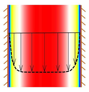
Figure 1. (a) A vertical channel with an exit slot. In (b,c), the exit slot is removed, and the periodic boundary conditions are applied in the  $y$- and
  $z$-directions. The walls are flat and frictional in (b), and are roughened by coating them with particles in a dense random packing in (c).
A granular material such as sand or glass beads is fed at the top of the channel and discharges through the exit slot at the bottom. It is assumed that the flow is steady and quantities do not vary in the  $z$-direction (figure 1a). Further, it is assumed that the flow is fully developed, so that quantities such as the velocity vary only in the
  $x$-direction. The velocity field is given by
 \begin{equation} u_x = 0 = u_z, \quad u_y = u_y(x). \end{equation}
Such a condition is expected to prevail at locations that are far from the upper free surface and the exit slot. This deceptively simple problem has been examined for several decades (Goodman & Cowin Reference Goodman and Cowin1971; Savage Reference Savage1979; Nedderman & Laohakul Reference Nedderman and Laohakul1980; Yalamanchili, Gudhe & Rajagopal Reference Yalamanchili, Gudhe and Rajagopal1994; Natarajan, Hunt & Taylor Reference Natarajan, Hunt and Taylor1995; Mohan, Nott & Rao Reference Mohan, Nott and Rao1997; Wang, Jackson & Sundaresan Reference Wang, Jackson and Sundaresan1997; Mohan et al. Reference Mohan, Nott and Rao1999; Pouliquen, Forterre & Le Dizes Reference Pouliquen, Forterre and Le Dizes2001; Ananda, Moka & Nott Reference Ananda, Moka and Nott2008), but a satisfactory model is lacking.
The DEM is a powerful tool to examine the mechanics of flowing granular materials, and has been used to study many systems such as hoppers (Zhao et al. Reference Zhao, Yang, Zhang and Chew2018), bunkers (Yu & Saxén Reference Yu and Saxén2010), vertical channels (González-Montellano, Ayuga & Ooi Reference González-Montellano, Ayuga and Ooi2011), inclined chutes (Bharathraj & Kumaran Reference Bharathraj and Kumaran2017, Reference Bharathraj and Kumaran2019) and circulating fluidized beds (Luo et al. Reference Luo, Wang, Yang, Hu and Fan2017). Data obtained from DEM simulations can be used to generate density, velocity and stress fields, which form vital benchmarks for comparison with the predictions of continuum models. Unlike the case of simple fluids such as air and water, there is no universally accepted constitutive equation for flowing granular materials. This topic has been examined for several decades, but the end is not in sight. Against this backdrop, it was felt that the proposed comparison of the predictions of continuum models with the results of DEM simulations for flow in a relatively simple geometry may serve to highlight the attractive features and defects of some of the recent models.
2. Details of the DEM
Following Cundall & Strack (Reference Cundall and Strack1979), the granular material is modelled as a collection of spherical grains that can overlap slightly. Here, we use a linear elastic spring and a viscous dashpot acting in parallel to determine the normal force  $N_f$ acting between two particles in contact (Cundall & Strack Reference Cundall and Strack1979; Shäfer, Dippel & Wolf Reference Shäfer, Dippel and Wolf1996). As the material is cohesionless,
  $N_f = 0$ when there is no overlap between the particles. A similar model is used for the tangential force
  $T_f$, but if
  $|T_f|/N_f > \mu _p$, the coefficient of interparticle friction,
  $|T_f|$ is replaced by
  $\mu _p N_f$, with a suitably chosen direction for
  $T_f$. Thus the contact forces are given by
 \begin{equation} \left.\begin{gathered} N_f ={-}k_n \delta_n \boldsymbol{n} - m_e \xi_n \boldsymbol{v}_n \\ T_f = \left\{\begin{array}{ll} -k_t \delta_t \boldsymbol{t} - m_e \xi_t \boldsymbol{v}_t, & {\rm if} \, \dfrac{\vert T_f \vert}{N_f} < \mu_p\\ -\mu_p N_f \boldsymbol{t}, & {\rm otherwise.} \end{array}\right. \end{gathered}\right\} \end{equation}
 In (2.1),  $\boldsymbol {n}$ and
  $\boldsymbol {t}$ denote the normal and tangential directions, respectively, where the former coincides with the direction of the line joining the centres of particles in contact,
  $k_n$ and
  $\xi _n$ are the spring constant and the damping constant in the normal direction, respectively,
  $\delta _n$ is the overlap in the normal direction and
  $\boldsymbol {v}_n$ is the normal component of the velocity at the contact point. For two particles of masses
  $m_1$ and
  $m_2$ that are in contact, the effective mass
  $m_e$ is defined by
 \begin{equation} m_e = \frac{m_1 m_2}{m_1 + m_2} . \end{equation}
 This approach is termed the linear spring and dashpot (LSD) model, and has been widely used (Silbert et al. Reference Silbert, Ertaş, Grest, Halsey, Levine and Plimpton2001; GDR-MiDi 2004; Chialvo, Sun & Sundaresan Reference Chialvo, Sun and Sundaresan2012; Guo & Curtis Reference Guo and Curtis2015). However, more sophisticated models for the contact force have also been used. For example, the classical Hertz model (Hertz Reference Hertz1882; Johnson Reference Johnson1987) predicts that  $N_f \propto \delta _n^{3/2}$. For tangential loading, the relation between
  $T_f$ and
  $\delta _t$ is more complicated (Johnson Reference Johnson1987; Vu-Quoc, Zhang & Lesburg Reference Vu-Quoc, Zhang and Lesburg2001). In some cases, results obtained with these models and the LSD model do not differ significantly (Di Renzo & Di Maio Reference Di Renzo and Di Maio2004; Kruggel-Emden et al. Reference Kruggel-Emden, Simsek, Rickelt, Wirtz and Scherer2007). Here, the simple LSD model is chosen as the benchmark for comparison, and computations are done using the open source code LAMMPS (Plimpton Reference Plimpton1995).
There are six parameters in the model for the contact forces between particles: the spring constants  $k_n$ and
  $k_t$, the damping constants
  $\xi _n$ and
  $\xi _t$, the coefficient of interparticle friction
  $\mu _p$ and the coefficient of particle–wall friction
  $\mu _w$. Following Debnath, Rao & Nott (Reference Debnath, Rao and Nott2017), we choose
  $k_n = 10^{6} \rho _p g d^{2}_p$,
  $k_t/k_n = 2/7$,
  $\xi _n = 180 \, \sqrt {g/d_p}$,
  $\xi _t/\xi _n = 1/2$ and
  $\mu _p = \mu _w = 0.5$, where
  $\rho _p$ and
  $d_p$ are the density and the diameter of the particle, respectively, and
  $g$ is the acceleration due to gravity. It is widely acknowledged that
  $k_n$ should be a few orders of magnitude larger for materials such as aluminium, stainless steel, brass and glass beads (see e.g. Mishra & Murty Reference Mishra and Murty2001; Silbert et al. Reference Silbert, Ertaş, Grest, Halsey, Levine and Plimpton2001; Kruggel-Emden et al. Reference Kruggel-Emden, Simsek, Rickelt, Wirtz and Scherer2007), but this would result in a very small time step being used when the equations of motion are integrated. The value chosen is believed to give reasonable results, and reflects a compromise between realistic parameter values and excessive computation time. The time step used is
 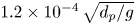 $1.2\times 10^{-4}\,\sqrt {d_p/g}$. Debnath et al. (Reference Debnath, Rao and Nott2017) estimated the lift on a disc immersed in a rotating bed of granular material, and found that modest changes in the value of
  $k_n$ by a factor of 10 do not affect the normal stresses exerted on the disc significantly. The value of
  $k_t/k_n$ is commonly used; it is obtained by considering an elastic collision between a sphere and a flat surface, assuming that the time periods for normal and tangential collisions are equal (Shäfer et al. Reference Shäfer, Dippel and Wolf1996). The chosen values of
  $k_n$ and
  $\xi _n$ imply that the coefficient of restitution in the normal direction is 0.7, and the value chosen for
  $\mu _p$ is typical of values for glass beads. The parameters for particle–wall interactions are chosen to be the same as for interparticle interactions.
As is common practice in DEM, we use a slightly polydisperse granular material, with sizes 0.9  $d_p$, 1
  $d_p$ and 1.1
  $d_p$, and having number fractions 0.3, 0.4 and 0.3, respectively. This is done to prevent the formation of ordered or ‘crystalline’ layers near the wall. Some computations were also done for monodisperse materials, and the results did not differ significantly. Only the results for polydisperse materials are presented here. As the lengths are scaled by
  $d_p$, velocities by
  $\sqrt {g d_p}$, time by
  $\sqrt {d_p/g}$ and forces by
  $\rho _p g d^{3}_p$,
  $d_p$ does not occur explicitly in the scaled equations and hence its actual value need not be specified. Without loss of generality,
  $\rho _p$,
  $d_p$ and
  $g$ are set to 1 in DEM.
The simulation box is a rectangular parallelepiped, with a bottom and four flat frictional walls, of dimensions  $2 \, W$,
  $H$ and
  $B$ in the
  $x$-,
$x$-,  $y$- and
  $z$-directions, respectively (figure 1a). Henceforth, such walls will be referred to as ‘smooth’ walls. The box is filled with particles by uniformly pouring them from the top, and allowing them to settle under the action of gravity. The mass flow rate of the material can be controlled by adjusting the width of the exit slot at the bottom (figure 1a). However, for a channel of realistic dimensions, the number of particles
  $N_p$ that can be handled by the code become excessive. As the flow is expected to be fully developed far above the exit slot, the motion of a reasonable number of particles, say
  $5\times 10^{4} \text {--} 2\times 10^{5}$, is simulated by applying periodic boundary conditions in the
  $y$- and
  $z$-directions. Thus there are no solid walls in the
  $y$- and
  $z$-directions, and no exit slot (figure 1b). Some approaches to incorporating the effect of the exit slot and the walls in the
  $z$-direction will be indicated briefly later. If a particle leaves the simulation box with a velocity
  $\boldsymbol {v}$, it re-enters at the top
  $y = H$, with the same velocity and the same values of
  $x$ and
  $z$. As noted by Allen & Tildesley (Reference Allen and Tildesley2017), the use of periodic boundary conditions suppresses spatial variations in the
  $y$- and
  $z$-directions on length scales that are comparable to the dimensions of the box. Results are presented here for
  $H = 30 \, d_p$,
  $B = 40\, d_p$ and values of
  $2\,W$ in the range
  $30\text {--}80\,d_p$. A few simulations were done with different dimensions, say
  $H = 30 \,d_p$ and
  $B = 20\,d_p$, and the results did not vary with
  $H$ and
  $B$. The flow properties vary with
  $x$-direction, as discussed in § 4. An empty head space volume (with rectangular cross-section of dimensions
  $2\,W \times B$, similar to that of the channel) is added at the top, and its height
  $\Delta H$ is adjusted such that a specified bulk solids fraction
  $\bar {\phi }$ is attained during flow. Here,
  $\bar {\phi }$ is defined as the ratio of the total volume of the material to the volume of the channel. For
  $N_p$ particles in the simulation box, the total volume of the particles is
 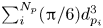 $\sum _{i}^{N_p} ({\rm \pi} /6) d^{3}_{p_i}$ and
  $2\,W \times B \times (H + \Delta H)$ is the volume of the simulation box. Some simulations are also done for the case of rough walls, where the walls are coated with a layer of stationary particles of diameter
  $d_p$ (figure 1c). The dimension
  $2\,W$ excludes the wall particles.
A preliminary study of Debnath, Kumaran & Rao (Reference Debnath, Kumaran and Rao2019) for flat frictional walls shows that there is no flow for  $\bar {\phi } > 0.62$. Steady flow occurs for
  $0.62 \geqslant \bar {\phi } \geqslant \bar {\phi }_{cr}$ and an oscillatory flow for
  $\bar {\phi }_{cr} > \bar {\phi } \geqslant \bar {\phi }_m$. Free fall under gravity occurs for
  $\bar {\phi } < \bar {\phi }_m$. Here,
  $\bar {\phi }_{cr}$ and
  $\bar {\phi }_m$ are parameters that depend on
  $2\,W/d_p$. The present work is confined to steady flow. A study on the transition to oscillatory flow and free fall will be discussed in a future work.
The simulation box is divided into bins of thickness  $1\, d_p$ in
  $x$-direction spanning over
  $(H + \Delta H)$ and
  $B$. The velocity and stresses in a bin are calculated by averaging the properties of particles whose centres are in that bin. The solids fraction
  $\phi$ is calculated as the ratio of the total volume of the material in a bin to the volume of the bin. The values of the properties are assigned to the centres of the bins. After
  $2\times 10^{7}$ time steps, when a steady and fully developed state is attained, the DEM results are time averaged over
  $5\times 10^{5}$ time steps. Except at the wall, the maximum distance
  $D_p$ between the centres of the particles in a bin is 1
  $d_p$. For the bin adjacent to the wall, if the bin width is
  $1 \, d_p$,
  $D_p$ is
  $(1/2) \, d_p$. To avoid this problem, the width of the bin adjacent to the wall is chosen as 1.5
  $d_p$. The standard deviation is very small compared with the sizes of the symbols representing the DEM results, and hence the error bars are not shown.
3. Continuum models
The classical frictional model for plane flow predicts a flat velocity profile, i.e. plug flow, with an indeterminate value for the velocity (Mohan et al. Reference Mohan, Nott and Rao1997). This is at variance with both experimental observations (Nedderman & Laohakul Reference Nedderman and Laohakul1980; Natarajan et al. Reference Natarajan, Hunt and Taylor1995; Pouliquen & Gutfraind Reference Pouliquen and Gutfraind1996; GDR-MiDi 2004; Ananda et al. Reference Ananda, Moka and Nott2008) and the DEM results to be discussed in this paper. These show shear layers near the channel walls and a plug layer near the centreline, and a lower value of the solids fraction  $\phi$ in the shear layer.
The model based on the kinetic theory of Lun et al. (Reference Lun, Savage, Jeffrey and Chepurniy1984) predicts results in good agreement with the measured velocity profiles when the centreline velocities are matched (Mohan et al. Reference Mohan, Nott and Rao1997), but  $\phi \approx \phi _{drp}$ in the plug layer, where the subscript
  $drp$ denotes dense random packing. Hence the underlying assumptions of kinetic theory, such as instantaneous collisions and molecular chaos, are likely to break down in this region. The frictional-kinetic model overcomes this defect by including frictional effects in the plug layer. However, the thickness of the shear layer is much less than that observed (Mohan et al. Reference Mohan, Nott and Rao1997).
An alternative approach is provided by the Cosserat plasticity model of Mohan et al. (Reference Mohan, Nott and Rao1999), wherein the symmetry of the stress tensor is relaxed and a balance for the couple stress is solved along with the other balances. The scaled velocity profile (velocity scaled by the centreline velocity) agrees fairly well with data. Thus this model appears to provide an elegant solution, but suffers from the defect that the profile of  $\phi$ is flat. Similarly, Pouliquen & Gutfraind (Reference Pouliquen and Gutfraind1996) developed a model based on stress fluctuations that fitted their data for the velocity profiles well, but
  $\phi$ was assumed to be constant. The qualitative observations of Natarajan et al. (Reference Natarajan, Hunt and Taylor1995) and experiments on two-dimensional flows comprised of circular cylindrical rods (Pouliquen & Gutfraind Reference Pouliquen and Gutfraind1996) suggest that the solids fraction
  $\phi$ is lower in the shear layer than near the centre.
Pouliquen (Reference Pouliquen1999) studied the flow of glass beads down an inclined chute with a rough base. He proposed a relation between the stress ratio  $\mu$ (the ratio of the shear stress to the normal stress), the mean velocity
  $u$ and the thickness
  $h$ of the flowing layer. Note that
  $\mu$ is a constant across the layer in this geometry. This relation is valid only for
  $h > h_{stop}$, where
  $h_{stop}$ is a critical thickness below which the flow stops abruptly. Pouliquen & Forterre (Reference Pouliquen and Forterre2002) examined the spreading of an initially hemispherical mass of glass beads down an inclined chute. The friction law of Pouliquen (Reference Pouliquen1999) was used, with some modifications for small values of
  $h$ to numerically solve depth-averaged equations. The predicted shape of the heap as a function of position and time matched their data well, except when the base had a static layer of material initially. Forterre & Pouliquen (Reference Forterre and Pouliquen2003) used both glass beads and sand, and fitted their data to the friction law
 \begin{equation} \frac{u}{\sqrt{g h}} ={-} \gamma_1 + \gamma_2 \, \frac{h}{h_{stop}(\theta)}, \end{equation}
where  $\gamma _1$ and
  $\gamma _2$ are constants,
  $g$ is the acceleration due to gravity and
  $\theta$ is the inclination of the chute to the horizontal. In particular,
  $\gamma _1 = 0$ for glass beads, but not for sand.
The group GDR-MiDi (2004) collated data and the results of DEM simulations from various geometries such as plane shear between horizontal plates in the absence of gravity, cylindrical Couette, inclined chute, vertical channel and rotating drum and from various papers. They found it helpful to introduce the inertial number  $I$, defined by
 \begin{equation} I = \frac{\vert S \vert \, d_p}{\sqrt{N/\rho_p}} , \end{equation}
where  $S$ is a suitable shear rate,
  $N$ is a suitable normal stress and
  $d_p$ and
  $\rho _p$ are the particle diameter and the particle density, respectively. The inertial number (or more precisely the square of
  $I$) is a rough measure of the ratio of the collisional stress to the total stress. Let
  $T$ denote a suitable shear stress. GDR-MiDi (2004) found that plane shear could be modelled by the relation
 \begin{equation} \mu = \mu (I), \end{equation}
where the friction coefficient or stress ratio is defined by
 \begin{equation} \mu \equiv \frac{\vert T \vert}{N} . \end{equation}
Equation (3.3) holds provided  $I$ is not too large. However, for inclined chutes, (3.3) was valid only for glass beads, but not for sand. This result follows from (3.1), with a non-zero value for
  $\gamma _1$. For rotating drums and heaps, the velocity profiles were not consistent with (3.3). Jop, Forterre & Pouliquen (Reference Jop, Forterre and Pouliquen2005) specified an explicit form for (3.3), and used it in their work (Jop, Forterre & Pouliquen Reference Jop, Forterre and Pouliquen2006) to solve the incompressible three-dimensional equations for flow down an inclined chute with rough sidewalls. For glass beads, good agreement was obtained between data and model predictions for the profile of the velocity at the free surface of the flowing layer.
Simulations reported in GDR-MiDi (2004) and Da Cruz et al. (Reference Da Cruz, Emam, Prochnow, Roux and Chevoir2005) show that
 \begin{equation} \phi = \phi(I), \end{equation}
where  $\phi$ is the solids fraction.
Another defect of (3.3) must be noted. Consider plane shear between horizontal plates, in the presence of gravity. If the upper plate is moved and the lower plate is stationary, this model predicts a shear layer near the moving plate, and a static bed of material near the lower plate. Pouliquen et al. (Reference Pouliquen, Cassar, Jop, Forterre and Nicolas2006) state that the thickness of the shear layer tends to zero in the limit of quasistatic flows ( $I \rightarrow 0$), whereas simulations show that it is of the order of 5–10
  $d_p$.
For plane flow, it has been shown that the incompressible  $\mu (I)$ model of Jop, Forterre & Pouliquen (Reference Jop, Forterre and Pouliquen2006) is linearly ill posed for small and large values of
  $I$ (Barker et al. Reference Barker, Schaeffer, Bohórquez and Gray2015). Here, ‘ill posed’ means that perturbations to the linearized unsteady equations grow at an unbounded rate as the wavelength of the perturbation tends to zero. By modifying the functional form of
  $\mu (I)$, Barker & Gray (Reference Barker and Gray2017) showed that the model is linearly well posed for
  $I < I_{max}$, where
  $I_{max}$ is a constant. Goddard & Lee (Reference Goddard and Lee2017) showed that the use of a higher gradient model (involving the fourth-order spatial derivatives of the velocity vector in the momentum balance) stabilizes the incompressible
  $\mu (I)$ model. We note in passing that the classical frictional model is ill posed for both incompressible flow (Schaeffer Reference Schaeffer1987) and compressible flow (Pitman & Schaeffer Reference Pitman and Schaeffer1987).
Consider the  $\mu (I) - \phi (I)$ class of models next. It has been shown (Heyman et al. Reference Heyman, Delannay, Tabuteau and Valance2017) that these are also ill posed for some flow conditions, but can be regularized by adding a term involving a quantity analogous to the bulk viscosity in the expression for the stress tensor. Let
  ${\boldsymbol{\mathsf{\sigma}}}$ denote the stress tensor, defined in the compressive sense, and
  $\boldsymbol{\mathsf{D}}$ the rate of deformation tensor, with components
 \begin{equation} {\mathsf{D}}_{ij} = \frac{1}{2} \left( {{\displaystyle \partial {u_i}} \over {\displaystyle \partial {x_j}}} + {{\displaystyle \partial {u_j}} \over {\displaystyle \partial {x_i}}} \right). \end{equation}
Goddard & Lee (Reference Goddard and Lee2018) have shown that the stress power  $\dot {\varPhi } = - {\boldsymbol{\mathsf{\sigma}}}: \boldsymbol{\mathsf{D}}$ is not always non-negative. Hence, this model is not pursued further. In any case, the bulk viscosity term vanishes for the velocity field considered here, and their model reduces to the
  $\mu (I)-\phi (I)$ model.
Another class of models is the higher gradient or ‘non-local’ models. The stresses at a point depend on the rate of deformation in a spatial region containing that point. There are many types of non-local models (Aranson & Tsimring Reference Aranson and Tsimring2001; Pouliquen et al. Reference Pouliquen, Forterre and Le Dizes2001; Pouliquen & Forterre Reference Pouliquen and Forterre2009; Wójcik & Tejchman Reference Wójcik and Tejchman2009; Henann & Kamrin Reference Henann and Kamrin2013; Bouzid et al. Reference Bouzid, Izzet, Trulsson, Clément, Claudin and Andreotti2015; Dsouza & Nott Reference Dsouza and Nott2020) and no single definition fits all of them. For example, Pouliquen et al. (Reference Pouliquen, Forterre and Le Dizes2001) and Pouliquen & Forterre (Reference Pouliquen and Forterre2009) assume that the shear rate at a point depends on the shear rates at other points, whereas Aranson & Tsimring (Reference Aranson and Tsimring2001) use an order parameter in the expression for the stress tensor. The order parameter is governed by a differential equation which describes the transition from solid-like to fluid-like behaviour. The model of Wójcik & Tejchman (Reference Wójcik and Tejchman2009) resembles that of Pouliquen & Forterre (Reference Pouliquen and Forterre2009), as the shear rate at a point is assumed to be a function of the weighted shear rates at neighbouring points. The models of Henann & Kamrin (Reference Henann and Kamrin2013) and Bouzid et al. (Reference Bouzid, Izzet, Trulsson, Clément, Claudin and Andreotti2015) are similar to the model of Aranson & Tsimring (Reference Aranson and Tsimring2001). Recently, Li & Henann (Reference Li and Henann2019) have shown that the incompressible model of Henann & Kamrin (Reference Henann and Kamrin2013) is well posed. However, the incompressible model of Bouzid et al. (Reference Bouzid, Izzet, Trulsson, Clément, Claudin and Andreotti2015) is not well posed even though higher gradients are included.
In this paper, the predictions of some of the recent well-posed models are compared with the results of simulations based on the DEM. Ill-posed behaviour is seen only when the models are used to solve the unsteady equations. The present work is an attempt to solve the steady state equations. For the models considered here, even the steady state aspects have not been studied in detail earlier in the context of flow through a vertical channel. It is hoped that the unsteady equations will be examined in the future.
3.1. Governing equations
The momentum balances for steady, fully developed flow are given by
 \begin{equation} \frac{\mbox{d} \sigma_{xx}}{\mbox{d}\kern0.7pt x} = 0; \quad \frac{\mbox{d} \sigma_{xy}}{\mbox{d}\kern0.7pt x} ={-} \rho_p \phi g , \end{equation}
where  $\sigma _{xx}$ and
  $\sigma _{xy}$ are the normal and shear stresses, defined in the compressive sense,
  $\rho _p$ is the particle density,
  $\phi$ is the solids fraction and
  $g$ is the acceleration due to gravity.
Expressing the stress components in terms of the principal stresses  $\sigma _1$ and
  $\sigma _2$, we obtain (Sokolovskii Reference Sokolovskii1965; Rao & Nott Reference Rao and Nott2008)
 \begin{equation} \sigma_{xx} = \sigma + \tau\cos (2\psi);\quad \sigma_{yy} = \sigma - \tau\cos (2\psi); \quad \sigma_{xy} ={-} \tau\sin (2\psi), \end{equation}
where
 \begin{equation} \sigma = \frac{\sigma_1 + \sigma_2}{2}; \quad \tau = \frac{\sigma_1 - \sigma_2}{2} .\end{equation}
Here,  $\sigma _1$ is the major principal stress, and
  $\psi$ is the inclination of the
  $\sigma _1$-axis relative to the
  $x$-axis (figure 1).
Thus (3.7a,b) and (3.8a–c) contain one more unknown than the number of equations. Before discussing closure of these equations, it is helpful to consider the more general case of flow parallel to the  $x$–
$x$– $y$ plane. In classical frictional models (see, for example, Mohan et al. (Reference Mohan, Nott and Rao1997)), the additional equations are provided by a yield condition
 \begin{equation} \tau = \tau(\sigma,\phi), \end{equation}
a flow rule
 \begin{equation} \cos(2\psi) \left( \frac{\partial u_y}{\partial y} + \frac{\partial u_x}{\partial x}\right) - \left(\frac{\partial \tau}{\partial \sigma}\right) \left( \frac{\partial u_y}{\partial y} - \frac{\partial u_x}{\partial x} \right) = 0 \end{equation}
and the coaxiality condition, which enforces the alignment of the principal axes of the stress and rate of deformation tensors
 \begin{equation} \cos(2\psi) \left( \frac{\partial u_x}{\partial y} + \frac{\partial u_y}{\partial x}\right) - \sin(2\psi) \left( \frac{\partial u_y}{\partial y} - \frac{\partial u_x}{\partial x} \right) = 0 . \end{equation}
In particular, (3.11) represents an associated flow rule.
3.2. The model of Barker et al. (Reference Barker, Schaeffer, Shearer and Gray2017)
Recently, Barker et al. (Reference Barker, Schaeffer, Shearer and Gray2017) have formulated a model for plane flow that is well posed by incorporating the inertial number  $I$ into the frictional equations described above. The coaxiality condition (3.12) is retained, but the yield condition and the flow rule are replaced by
 \begin{equation} \tau = Y(\sigma, \phi,I); \quad \left( {{\displaystyle \partial {u_x}} \over {\displaystyle \partial {x}}} + {{\displaystyle \partial {u_y}} \over {\displaystyle \partial {y}}} \right) = f(\sigma,\phi,I) S^{\prime},\end{equation}
where  $S^{\prime }$ is an equivalent shear rate, defined by
 \begin{equation} S^{\prime} = \sqrt{2 {\mathsf{D}}^{\prime}_{ij} {\mathsf{D}}^{\prime}_{ji}} ,\end{equation}
and
 \begin{equation} {\mathsf{D}}^{\prime}_{ij} = \frac{1}{2} \left( {{\displaystyle \partial {u_i}} \over {\displaystyle \partial {x_ j}}} + {{\displaystyle \partial {u_j}} \over {\displaystyle \partial {x_i}}} \right) - \frac{1}{2} \, {{\displaystyle \partial {u_k}} \over {\displaystyle \partial {x_k}}} \, \delta_{ij}. \end{equation}
Here, repeated indices imply summation, and  $\delta _{ij}$ is the Kronecker delta. The form of the coaxiality condition given in Barker et al. (Reference Barker, Schaeffer, Shearer and Gray2017) differs from (3.12), but can be shown to be equivalent after some manipulations. The alternative form is also discussed in § 3 of Barker et al. (Reference Barker, Schaeffer, Shearer and Gray2017).
Because of the incorporation of  $I$, (3.13a,b) does not represent classical frictional behaviour. However, for ease of exposition, we retain the terms ‘yield condition’ and ‘flow rule’.
For the equations to be well posed, the yield function  $Y$ and flow rule function
  $f$ are required to satisfy certain conditions. To relate these equations to the
  $\mu (I)$ model, Barker et al. (Reference Barker, Schaeffer, Shearer and Gray2017) proposed the forms
 \begin{equation} \left.\begin{gathered} \tau = Y(\sigma,\phi,I) = \alpha (I) \sigma - \frac{\sigma^{2}}{C(\phi)} \\ f(\sigma, \phi, I) = \beta(I) - \frac{2 \sigma}{C(\phi)} \end{gathered}\right\}, \end{equation}
where  $\sigma$ is the mean stress defined by (3.9a,b) and
 \begin{equation} \left.\begin{gathered} \alpha (I) = \frac{4}{5} \mu (I) + \frac{12}{25} \, I^{{-}2/5}\int_{0}^{I} j^{{-}3/5} \mu(j)\,{\rm d}j \\ \beta (I) ={-}\frac{2}{5} \mu (I) + \frac{24}{25} \, I^{{-}2/5}\int_{0}^{I} j^{{-}3/5} \mu(j)\,{\rm d}j \\ C(\phi) = \varLambda \frac{\phi-\phi_{min}}{\phi_{max} - \phi}, \end{gathered}\right\} \end{equation}
where  $\varLambda$,
  $\phi _{min}$ and
  $\phi _{max} > \phi _{min}$ are material constants. The form suggested by Barker et al. (Reference Barker, Schaeffer, Shearer and Gray2017) for
  $C (\phi )$ is only representative of a function that increases monotonically with
  $\phi$, and has not been deduced from experimental data. It is identical in form to the expression proposed by Savage & Sayed (Reference Savage and Sayed1979) for the mean stress at a critical state or a state of isochoric deformation.
For the problem at hand, the coaxiality condition (3.12) reduces to
 \begin{equation} \frac{\mbox{d} u_y}{\mbox{d} x} \cos (2 \psi) = 0, \end{equation}
and (3.2) to
 \begin{equation} I = \frac{d_p \, \dfrac{\mbox{d} u_y}{\mbox{d} x} }{\sqrt{\sigma_{xx}/\rho_p}}, \end{equation}
where the shear rate  $S$ and the normal stress
  $N$ in (3.2) have been identified with
  $\mbox {d} u_y/ \mbox {d} x$ and
  $\sigma _{xx}$, respectively. Similarly, (3.4) is replaced by
 \begin{equation} \mu(I) = \frac{\vert \sigma_{xy} \vert}{\sigma_{xx}} . \end{equation}
 As noted by Mohan et al. (Reference Mohan, Nott and Rao1997), either (i)  $\mbox {d} u_y/\mbox {d} x = 0$, or (ii)
  $\psi = \underline {+} {\rm \pi}/4$. If (i) holds, the material moves as a plug, and there are no shear layers near the walls of the channel. This is at variance with experimental observations and the results of DEM simulations. Hence, this root must be discarded, except possibly for a plug layer near the centre of the channel.
Considering the other roots (ii), the choice  $\psi = -{\rm \pi} /4$ is ruled out as it implies that
  $\sigma _{xy} = \tau \geqslant 0$. Hence, if
  $\tau \neq 0$ at the wall
  $x = W$, the material flowing downward will exert an upward shear stress on the wall. This behaviour is unrealistic and must be avoided.
The other choice is  $\psi = {\rm \pi}/4$, which along with (3.8a–c) implies that
 \begin{equation} \sigma_{xx} = \sigma_{yy} = \sigma; \quad \sigma_{xy} ={-}\tau . \end{equation}
At the centre  $x = 0$, the velocity profile must be symmetric, and hence
  $\mbox {d} u_y/\mbox {d} x = 0$. Similarly, the shear stress
  $-\sigma _{xy} (x = 0) = \tau (x = 0) = 0$. Equation (3.19) implies that
  $I(0) = 0$, and the data of Jop, Forterre & Pouliquen (Reference Jop, Forterre and Pouliquen2005) show that
  $\mu (0) = \mu _s > 0$. It follows from (3.20) that
  $\tau (0) = \mu _s \sigma (0) = 0$, or
  $\sigma (0) = 0$. However, the momentum balance (3.7a,b) and this result imply that
  $\sigma _{xx} = \sigma = 0$ even at the wall, which is unrealistic. Hence, neither of the roots
  ${\textrm {d}u_y}/{\textrm {d} x} = 0$ and
  $\psi = {\rm \pi}/4$ apply throughout the domain
  $0 < x < W$.
One approach to resolve this problem is to postulate a plug layer of thickness  $x_p$ near the centre, where
  $\mbox {d} u_y/\mbox {d}x = 0$, and a shear layer of thickness
  $(W - x_p)$ near the wall. In the shear layer,
  $\psi = {\rm \pi}/4$ and appropriate matching conditions are used at the interface
  $x = x_p$. A similar approach was used by Mohan et al. (Reference Mohan, Nott and Rao1997) for the frictional-kinetic equations.
In the plug layer  $(0 \leqslant x \leqslant x_p)$, the material does not deform and the solids fraction
  $\phi$ is assumed to be a constant
  $\equiv \phi _p$. The momentum balances imply that
 \begin{equation} \left.\begin{gathered} \sigma_{xx} = {\rm const.} = \sigma + \tau\cos (2\psi) \equiv N\\ - \sigma_{xy} = \tau \sin (2\psi) = (\rho_pg\phi_p) x \end{gathered}\right\}.\end{equation}
 In the shear layer  $(x_p < x \leqslant W)$,
  $\psi = {\rm \pi}/4$ and the momentum balances reduce to
 \begin{equation} \left.\begin{gathered} \sigma_{xx} = {\rm const.} = \sigma = N \\ \frac{\mbox{d} \tau}{\mbox{d} x} = \rho_p \phi g \end{gathered}\right\},\end{equation}
where (3.21a,b) has been used. As  $\partial u_k/\partial x_k = 0$, the flow rule (3.13b) reduces to
  $f = 0$, or using (3.16)
 \begin{equation} \sigma = N = \beta(I) C(\phi)/2. \end{equation}
Applying the above conditions and using (3.16)
 \begin{equation} \tau = Y(\sigma,\phi,I) = \mu(I) \sigma = \mu(I)N. \end{equation}
An explicit expression is needed for  $\mu (I)$; here, we use the expression of Jop, Forterre & Pouliquen (Reference Jop, Forterre and Pouliquen2005), which is given by
 \begin{equation} \mu(I) = \mu_s + \frac{\Delta \mu}{(I_0/I) + 1} ,\end{equation}
where  $\mu _s$,
  $\Delta \mu$, and
  $I_0$ are positive constants. Equation (3.24) is linear in
  $\phi$, and can be solved to obtain
 \begin{equation} \phi = \frac{ \beta(I) \varLambda \phi_{min}+ 2 N \phi_{max}}{\beta(I) \varLambda + 2 N} . \end{equation}
 Using (3.27), (3.17) and (3.26), (3.23) is integrated from  $x = x_p$ to
  $x = W$ with the initial condition
 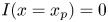 $I(x = x_p) = 0$. The MATLAB routine ODE45 is used for numerical integration, and the integral in the expression for
  $\beta (I)$ in (3.17) is evaluated using Gauss–Legendre four point quadrature. In the limit
  $I \rightarrow 0$, the integral can be evaluated analytically, giving
  $\beta (I) = 2\mu _s$.
To obtain the thickness  $x_p$ of the plug layer, the stresses and the velocity gradient at
  $x_p^{-}$ must be matched to the corresponding values at
  $x_p^{+}$. At
  $x = x_p$,
  $I(x_p)=0$ and
 \begin{align} -\sigma_{xy}(x = x_p^{-}) &= (\rho_p \phi_p g ) x_p ={-}\sigma_{xy}(x = x_p^{+}) \nonumber\\ &= \tau = \mu(I(x = x_p)) \sigma = \mu(I(x = x_p)) N. \end{align}
As  $I(x_p^{-}) = 0$, (3.26) and (3.28) imply that
  $\mu (x = x_p) = \mu _s$. Substituting
  $I = 0$,
  $\phi _p$ can be obtained from (3.27), and hence
 \begin{equation} x_p = \frac{\mu_s N}{\rho_p \phi_p g } . \end{equation}
Equation (3.19) implies that the velocity profile is governed by
 \begin{equation} \frac{\mbox{d} u_y}{\mbox{d} x} = \frac{I}{d_p}\, \sqrt{\frac{N}{\rho_p}} . \end{equation}
 As there is one unknown parameter, namely, the normal stress  $N$, and one condition is needed to integrate (3.30), two conditions have to be specified. Here, the bulk solids fraction
 \begin{equation} \bar{\phi} \equiv \frac{1}{W} \int_{0}^{W} \phi \, \mbox{d} x ,\end{equation}
and the mass flow rate
 \begin{equation} \dot{M}\equiv 2 \rho_p B \int_{0}^{W} (- u_y) \phi \, \mbox{d} x , \end{equation}
where  $B$ is the thickness of the channel in the
  $z$-direction (figure 1), are matched to the DEM results.
In the DEM,  $\dot {M}$ is fixed by specifying
  $\bar {\phi }$ for a fixed value of
  $2\,W$, but it appears that for the continuum models, both the parameters can be specified independently. In the latter case, the additional degree of freedom arises because we are unaware of a suitable velocity or stress boundary condition (b.c.) that can be specified at the wall.
For example, a modified form of the b.c. proposed by Mohan et al. (Reference Mohan, Nott and Rao1999) is given by
 \begin{equation} u_y(x=W) - u_{wall} ={-} l_u \,\frac{\mbox{d} u_y}{\mbox{d} x} , \end{equation}
where  $u_{wall}$ is the velocity of the wall and
  $l_u$ is a material parameter called the slip length. In our case,
  $u_{wall} = 0$. Equation (3.33) is due to Tejchman & Gudehus (Reference Tejchman and Gudehus1993) and Tejchman & Wu (Reference Tejchman and Wu1993), who expressed it in terms of displacement and rotation. Subsequently, Mohan et al. (Reference Mohan, Nott and Rao1999, Reference Mohan, Rao and Nott2002) rewrote it in terms of the velocity and the angular velocity
  $\omega$. As noted by Batchelor (Reference Batchelor1967),
  $\omega$ is equal to half the vorticity
  $\mbox {d} u_y/ \mbox {d} x$ for a classical continuum. However, the value of
  $l_u$ is not known a priori. Hence it is calculated using (3.33) after the velocity field has been obtained. We shall see later that
  $l_u$ varies with
  $\bar {\phi }$ and the channel width
  $2\,W$ for the models used here, and hence (3.33) is not a realistic b.c. for most of the models.
There are similar reservations about the wall friction b.c.
 \begin{equation} \mu(x=W) = \mu_w = \frac{-\sigma_{xy}(x = W)}{N} = \frac{\tau(x = W)}{N} = \tan \delta, \end{equation}
where (3.21a,b) has been used and  $\delta$ is called the angle of wall friction. Equation (3.34) has been commonly used in the in the literature on slow flow (Brennen & Pearce Reference Brennen and Pearce1978; Nedderman et al. Reference Nedderman, Tüzün, Savage and Houlsby1982; Dsouza & Nott Reference Dsouza and Nott2020) but may not be appropriate when the inertial effects are important near the wall. Integrating the second of (3.7a,b) from
  $x = 0$ to
  $x = W$ using an initial condition
  $\sigma _{xy} (x = 0) = 0$, and using (3.31) and (3.34)
 \begin{equation} \tan \delta = \frac{\bar{\phi}}{\tilde{N}} , \end{equation}
where  $\tilde {N} = N/ (\rho _p gW)$.
The model of Barker et al. (Reference Barker, Schaeffer, Shearer and Gray2017) differs from  $\mu (I)-\phi (I)$ model as it is shown to be well posed, and (3.27) implies that
  $\phi$ depends on
  $I$ and the normal stress
  $N$.
$N$.
3.3. The model of Schaeffer et al. (Reference Schaeffer, Barker, Tsuji, Gremaud, Shearer and Gray2019)
This builds on the work of Barker et al. (Reference Barker, Schaeffer, Shearer and Gray2017), by proposing an ad hoc expression for the yield function  $Y$ and deducing the expression for the flow rule function
  $f$. It is shown that the resulting equations are well posed. Thus this model involves fewer assumptions than that of Barker et al. (Reference Barker, Schaeffer, Shearer and Gray2017), as the latter proposes ad hoc expressions for both
  $Y$ and
  $f$.
$f$.
Schaeffer et al. (Reference Schaeffer, Barker, Tsuji, Gremaud, Shearer and Gray2019) conducted gravity-free DEM simulations of the plane shear of discs, and found that  $\mu = \mu (I)$. They fitted the data to (3.26), thereby determining the values of
  $\mu _s$,
  $\Delta \mu$ and
  $I_0$. They also found that
 \begin{equation} I = \varPsi (\phi) \equiv \frac{\phi_c - \phi}{a} , \end{equation}
where  $\phi _c$ and
  $a$ are constants. We shall use different data for parameter estimation as our grains are assumed to be spherical.
Retaining the coaxiality condition (3.12), a new yield condition dependent on  $I$,
$I$,  $\sigma$ and
  $\varPsi$ is chosen as
 \begin{equation} \tau = Y(\sigma, I, \phi) = \mu(\varPsi (\phi)) \sigma \frac{I}{\varPsi (\phi)} . \end{equation}
 Note that  $I \neq \varPsi (\phi )$ in general. The
  $\mu (I) - \phi (I)$ model is recovered in cases where
  $I = \varPsi (\phi )$. To make the system well posed, it turns out that (Barker et al. Reference Barker, Schaeffer, Shearer and Gray2017)
 \begin{equation} f(\sigma, I, \phi) = f(I,\phi) = \frac{1}{4}\; \mu(\varPsi(\phi)) \left( \frac{I}{\varPsi(\phi)} - \frac{\varPsi(\phi)}{I} \right) . \end{equation}
 For steady, fully developed flow  $\partial u_k/\partial x_k = 0$. Hence, (3.13b) and (3.38) imply that
 \begin{equation} I = \varPsi (\phi) . \end{equation}
Using (3.36), we obtain
 \begin{equation} \phi = \phi_c - aI. \end{equation}
For this special case, the model of Schaeffer et al. (Reference Schaeffer, Barker, Tsuji, Gremaud, Shearer and Gray2019) is identical to the  $\mu (I) - \phi (I)$ model. However, they have shown that for unsteady one-dimensional flow, the model leads to well-posed behaviour of the numerical solutions, in contrast to the
  $\mu (I) - \phi (I)$ model.
To the best of our knowledge, the only other papers that have applied the  $\mu (I) - \phi (I)$ model to channel flow are those of Pouliquen et al. (Reference Pouliquen, Forterre and Le Dizes2001) and Pouliquen et al. (Reference Pouliquen, Cassar, Jop, Forterre and Nicolas2006). The present work differs from theirs in the following respects: (i) they use a no-slip condition at the wall, whereas we permit slip, (ii) they state that the shear stress
  $\tau$ and hence the friction coefficient
  $\mu = \tau /N$ vary linearly with
  $x$, whereas we find that this is not an exact result but holds to a good approximation, (iii) results are presented here for a range of channel widths
  $2\,W$ and bulk solids fractions
  $\bar {\phi }$, but only for one value of
  $\bar {\phi }$ and an unspecified value of
  $2\,W$ in their work, (iv) as experimental data and DEM results were not available at that time, model predictions could not be compared with these in their work, whereas extensive comparisons with DEM results are presented here. However, we greatly appreciate their efforts to solve this problem.
Using (3.26) and (3.40), and noting that  $\tau = \mu (I) N$, the momentum balance (3.23) is integrated from
  $x_p$ to
  $W$ with the initial condition
  $I(x = x_p) = 0$. The solids fraction in the plug layer is given by
  $\phi _p = \phi _c$ as
  $I = 0$ (see (3.36) and the thickness of the plug layer is given by (3.29). This implicitly assumes that the DEM results used to deduce the forms of
  $\mu (I)$ and
  $\phi (I)$ are valid in the limit
  $I \rightarrow 0$, even though the smallest value of
  $I$ for the results is about 0.002. The form (3.40) permits the momentum balance (3.23) to be integrated analytically, resulting in
 \begin{equation} \frac{1}{(I_0+(\phi_c/a))^{2}} \ln\left|\frac{I_0+I}{(\phi_c/a)-I} \right| - \frac{1}{(I_0+(\phi_c/a))(I_0+I)} = \frac{a}{I_0\Delta \mu} \frac{\rho_pg x}{N} + k , \end{equation}
where the integration constant  $k$ is evaluated by using the initial condition
  $I(x_p) = 0$. The solids fraction is obtained using (3.40), and
  $N$ by matching
  $\bar {\phi }$ to the DEM result. To obtain the velocity profile, (3.30) is integrated using (3.41) similarly, as discussed in § 3.2.
3.4. The model of Henann & Kamrin (Reference Henann and Kamrin2013)
For three-dimensional flow, Henann & Kamrin (Reference Henann and Kamrin2013) define an equivalent shear stress by
 \begin{equation} \tau^{\prime} = (\sigma^{\prime}_{ij} \sigma^{\prime}_{ji} / 2)^{1/2} ,\end{equation}
where
 \begin{equation} \sigma^{\prime}_{ij} \equiv \sigma_{ij} - p \delta_{ij}; \quad p \equiv \sigma_{kk}/3 ,\end{equation}
and  $p$ is the mean stress or the pressure. Their constitutive equation is given by
 \begin{equation} \sigma_{ij} = p \delta_{ij} - 2 \frac{p}{f} \,{\mathsf{D}}_{ij}, \end{equation}
where the stresses are defined in the compressive sense and the quantity  $f$ is called the granular fluidity. It is defined by
 \begin{equation} f \equiv S^{\prime}/\mu ,\end{equation}
where the shear rate  $S^{\prime }$ is defined by (3.14), with (3.15) replaced by
 \begin{equation} {\mathsf{D}}^{\prime}_{ij} = \frac{1}{2} \left({{\displaystyle \partial {u_i}} \over {\displaystyle \partial {x_ j}}} + {{\displaystyle \partial {u_j}} \over {\displaystyle \partial {x_i}}} \right) - \frac{1}{3}\, {{\displaystyle \partial {u_k}} \over {\displaystyle \partial {x_k}}} \, \delta_{ij}, \end{equation}
and
 \begin{equation} \mu \equiv \tau^{\prime}/p . \end{equation}
Here,  $\tau ^{\prime }$ is given by (3.42).
Because  $f$ is governed by a differential equation, this model is called a non-local model in the sense of GDR-MiDi (2004). At a steady state, this equation is assumed to be given by (Kamrin & Henann Reference Kamrin and Henann2015; Zhang & Kamrin Reference Zhang and Kamrin2017)
 \begin{equation} A^{2} d_p^{2} \nabla^{2} f = \Delta \mu \left( \frac{\mu_s - \mu}{\mu_s + \Delta \mu - \mu} \right) f + \frac{\Delta \mu}{I_0} \, \sqrt{\frac{\rho_p d_p^{2}}{p}}\, \mu f^{2} , \end{equation}
where  $I_0$,
  $\Delta \mu$,
  $\mu _s$ and
  $A$ are constants.
Equation (3.48) differs from the equation used by Kamrin & Koval (Reference Kamrin and Koval2012) and Henann & Kamrin (Reference Henann and Kamrin2013), who linearized the term involving  $f^{2}$ about a local value of the fluidity
  $f_{loc}$. The latter was assumed to be a function of the inertial number
  $I$. As suggested by one of the referees, we use the more complete form (3.48). Thus the present analysis deals with a modified version of the model of Henann & Kamrin (Reference Henann and Kamrin2013). They assume that
  $\phi = \textrm {const}.$, which is a drawback of the model. They suggested that
  $\phi$ could be treated as a function of
  $I$, thereby relaxing this constraint. However, it was not implemented in their paper. Some results obtained with
  $\phi = \phi (I)$ are presented here.
Let us now consider the case of steady, fully developed flow. Equation (3.44) implies that
 \begin{equation} \sigma_{xx} = \sigma_{yy} = \sigma_{zz} = p; \quad \sigma_{xy} = \sigma_{yx} ={-} \frac{ p }{f} \, \frac{\mbox{d} u_y}{ \mbox{d} x}. \end{equation}
Using (3.49a,b), the momentum balances reduce to
 \begin{equation} p = \mbox{const.} \equiv N; \quad\frac{\mbox{d}}{\mbox{d} x} \left( \frac{ p }{f} \, \frac{\mbox{d} u_y}{ \mbox{d} x} \right) = \rho_p \phi g. \end{equation}
 Integrating (3.50b) with  $\phi = \textrm {const}. = \phi _p$ and using the b.c. of vanishing shear stress at
  $x = 0$, we obtain
 \begin{equation} \frac{N}{f} \frac{\mbox{d} u_y}{\mbox{d} x} = \rho_p\, \phi_p g x . \end{equation}
Henceforth,  $\phi _p$ is set equal to the bulk solids fraction
  $\bar {\phi }$ obtained from the DEM results.
Using (3.42), (3.47), (3.49a,b) and (3.51), we obtain
 \begin{equation} \mu = \frac{\vert \sigma_{xy} \vert}{p} = \left \vert \frac{1}{f} \, \frac{ \mbox{d} u_y}{\mbox{d} x} \right \vert = \frac{1}{f} \, \frac{ \mbox{d} u_y}{\mbox{d} x} = \frac{\rho_p \phi_p g }{N} x ,\end{equation}
as  $\mbox {d} u_y/\mbox {d} x$ is expected to be
  ${\geqslant }0$ for downward flow, and
  $f$ should be non-negative (see (3.45)).
The equation for the fluidity (3.48) reduces to
 \begin{equation} \frac{ \mbox{d}^{2} f}{ \mbox{d} x^{2}} = \frac{\Delta \mu}{A^{2} d_p^{2}} \left( \frac{\mu_s - \mu}{\mu_s + \Delta \mu - \mu} \right) f + \frac{\Delta \mu}{I_0 A^{2} d_p^{2}} \, \sqrt{\frac{\rho_p d_p^{2}}{N}} \mu f^{2} . \end{equation}
Two b.c.s are needed for (3.53). Henann & Kamrin (Reference Henann and Kamrin2013) assume that the gradient of  $f$ in the direction normal to a boundary vanishes. Here, it implies that
  $\mbox {d} f/\mbox {d} x = 0$ at the walls
  $x = \underline {+} W$. As (3.53) is solved only in the region
  $0 \leqslant x \leqslant W$, let us consider the b.c. at
  $x = 0$ first. The vertical velocity
  $u_y$ is expected to be an even function of
  $x$. Expanding
  $u_y$ in a Taylor series about
  $x = 0$, we obtain
 \begin{equation} u_y = a + b x^{2} + {O}(x^{4}); \quad x \rightarrow 0 , \end{equation}
where  $a$ and
  $b$ are constants. Hence the shear rate
  $S^{\prime }$ is given by
  $S^{\prime } = 2 b x + {O} (x^{3})$. Using this result along with (3.45) and (3.52), we obtain
 \begin{equation} f = \frac{2 b}{c} + {O}(x^{2}); \quad x \rightarrow 0 , \end{equation}
where  $c$ is a constant. Hence one b.c. is given by
 \begin{equation} \frac{ \mbox{d} f}{ \mbox{d} x} (0) = 0 . \end{equation}
As a physically appealing b.c. is lacking at  $x = W$, we follow Zhang & Kamrin (Reference Zhang and Kamrin2017) and set
 \begin{equation} f (x = W) \equiv f_w = f_{dem} , \end{equation}
where  $f_{dem}$ is the value of
  $f$ obtained from the DEM results. By analogy with the slip b.c. (3.33), a possible alternative b.c. for
  $f_w$ may be
 \begin{equation} f_w = l_f \left\vert \frac{\mbox{d}f}{\mbox{d}\kern0.7pt x}\right\vert , \end{equation}
where  $l_f$ is a slip length associated with the fluidity. Values of
  $l_f$ are obtained from the DEM results and the model predictions, as discussed in § 4.4.
The MATLAB routines ODE45 and FSOLVE are used to integrate (3.53) and for iterative matching of the b.c.s, respectively. Here,  $\phi _p$ is chosen as
  $\bar {\phi }$, which is consistent with the selection for comparisons with the DEM and the other models. To obtain the velocity profile, (3.51) has to be integrated, and two more conditions are needed as the normal stress
  $N$ is not known a priori. Because of the lack of appropriate b.c.,
  $N$ and the mass flow rate
  $\dot {M}$ are matched to the DEM results. The structure of (3.53) and the b.c. permits an approximate solution, as discussed in § 4.4.2.
To relax the assumption that  $\phi = \textrm {const}.$, some results are also presented with
  $\phi = \phi (I)$, where the functional form (3.40) is used. The equations will be solved in similarly, as discussed in § 3.2, and
  $N$ will be predicted by matching
  $\bar {\phi }$ to the DEM results.
As noted by one of the referees, (3.53) has been solved earlier by Zhang & Kamrin (Reference Zhang and Kamrin2017). However, the friction coefficient  $\mu$ has been taken from the DEM results (K. Kamrin, private communication 2021), and hence it is not a complete solution of the model equations (3.49a,b), (3.50a,b), (3.52) and (3.53). There is no mention of the
  $\phi$ and
  $u_y$ profiles in their paper, a gap that has been filled in the present work. Some other aspects of this model are discussed in § 4.4.
3.5. The model of Dsouza & Nott (Reference Dsouza and Nott2020)
Dsouza & Nott (Reference Dsouza and Nott2020) start with the classical frictional model that involves a yield condition and a flow rule (Srivastava & Sundaresan Reference Srivastava and Sundaresan2003; Rao & Nott Reference Rao and Nott2008). Integrating the flow rule over a representative volume with an effective radius  $\ell$, and ignoring terms of
  ${O}(\ell ^{4})$ and higher in the stresses, the constitutive equations are given by
 \begin{equation} \left.\begin{gathered}
\sigma_{ij} = p \delta_{ij} - \frac{2 \mu_*}{S^{\prime}} (
p_c {\mathsf{D}}'_{ij} - \ell^{2} \varPi \nabla^{2} {\mathsf{D}}'_{ij} ) \\ p_c =
\varPi - \ell^{2} \, \frac{\mbox{d} \varPi}{\mbox{d} \phi}
\, \nabla^{2}\phi \\ p = p_c \left( 1-
\frac{\mu_b}{S^{\prime}} \, \boldsymbol{\nabla}
\boldsymbol{\cdot} \boldsymbol{u} \right) + \ell^{2} \varPi
\frac{\mu_b}{S^{\prime}} \nabla^{2} \, \boldsymbol{\nabla}
\boldsymbol{\cdot} \boldsymbol{u}
\end{gathered}\right\},
\end{equation}
\begin{equation} \left.\begin{gathered}
\sigma_{ij} = p \delta_{ij} - \frac{2 \mu_*}{S^{\prime}} (
p_c {\mathsf{D}}'_{ij} - \ell^{2} \varPi \nabla^{2} {\mathsf{D}}'_{ij} ) \\ p_c =
\varPi - \ell^{2} \, \frac{\mbox{d} \varPi}{\mbox{d} \phi}
\, \nabla^{2}\phi \\ p = p_c \left( 1-
\frac{\mu_b}{S^{\prime}} \, \boldsymbol{\nabla}
\boldsymbol{\cdot} \boldsymbol{u} \right) + \ell^{2} \varPi
\frac{\mu_b}{S^{\prime}} \nabla^{2} \, \boldsymbol{\nabla}
\boldsymbol{\cdot} \boldsymbol{u}
\end{gathered}\right\},
\end{equation}
where  $\mu _*$ and
  $\mu _b$ are constants,
  $S^{\prime }$ is defined by (3.14),
  ${\mathsf{D}}^{\prime }_{ij}$ by (3.46),
  $\boldsymbol {u}$ is the velocity vector and
  $p = \sigma _{kk}/3$ is the mean stress or the pressure. The variable
  $p_c$ in (3.59) is the mean stress at a critical state or a state of isochoric motion, and
  $\varPi (\phi )$ is its ‘local’ contribution. A suitable form must be specified for
  $\varPi (\phi )$, and it is chosen as (Savage & Sayed Reference Savage and Sayed1979)
 \begin{equation} \varPi (\phi) = \varLambda^{*} \, \frac{\phi - \phi_{min}}{\phi_{max} - \phi}, \ \phi \geqslant \phi_{min}; \quad \varPi = 0, \ \phi \leqslant \phi_{min} , \end{equation}
where  $\varLambda ^{*}$,
  $\phi _{min}$ and
  $\phi _{max} > \phi _{min}$ are material constants. Dsouza & Nott (Reference Dsouza and Nott2020) use the expression proposed by Johnson, Nott & Jackson (Reference Johnson, Nott and Jackson1990)
 \begin{equation} \varPi (\phi) = \varLambda^{\prime} \,\frac{(\phi - \phi_{min})^{2}}{(\phi_{max} - \phi)^{5}}, \ \phi \geqslant \phi_{min}; \quad \varPi = 0, \ \phi \leqslant \phi_{min} , \end{equation}
where  $\varLambda ^{\prime }$ is a material constant. The latter form diverges faster as
  $\phi \rightarrow \phi _{max}$ than the former. Here, we use (3.60) to solve this model. The effect of (3.61) on the predictions is discussed in § 4.
Because of the integration of the flow rule over a volume, (3.59) may be regarded as a non-local model. The authors state, but do not prove, that the model is linearly well posed.
As  $\boldsymbol {\nabla }\boldsymbol {\cdot } \boldsymbol {u} = 0$ for the velocity field (1.2a,b), (3.59) reduces to
 \begin{equation} \left.\begin{gathered} \sigma_{xx} = \sigma_{yy} = \sigma_{zz} = p = p_c = \varPi - \ell^{2} \, \frac{\mbox{d} \varPi}{\mbox{d} \phi} \, \frac{\mbox{d}^{2} \phi}{\mbox{d} x^{2}} \\ \sigma_{xy} = \sigma_{yx} ={-} \frac{ \mu_*}{S^{\prime}} \left( p_c \, \frac{ \mbox{d} u_y}{\mbox{d} x} - \ell^{2} \varPi \, \frac{\mbox{d}^{3} u_y}{\mbox{d} x^{3}} \right) \end{gathered}\right\}, \end{equation}
where
 \begin{equation} S^{\prime} = \frac{ \mbox{d} u_y}{\mbox{d} x}. \end{equation}
Using (3.62), the momentum balances reduce to
 \begin{equation} \left.\begin{gathered} p = p_c = \varPi - \ell^{2} \, \frac{\mbox{d} \varPi}{\mbox{d} \phi} \, \frac{\mbox{d}^{2} \phi}{\mbox{d} x^{2}} = \mbox{const}. \equiv N \\ \frac{\mbox{d} \sigma_{xy}}{\mbox{d} x} ={-} \frac{ \mbox{d}}{\mbox{d} x} \left( \frac{ \mu_*}{S^{\prime}} \left( p_c \, \frac{ \mbox{d} u_y}{\mbox{d} x} - \ell^{2} \varPi \, \frac{\mbox{d}^{3} u_y}{\mbox{d} x^{3}} \right) \right) ={-} \rho_p \phi g \end{gathered}\right\}. \end{equation}
 To solve (3.64), seven conditions are needed as the normal stress  $N$ is unknown a priori. The first of (3.64) depends only on
  $\phi$, and hence is solved separately using the MATLAB routine ODE45. Due to the lack of appropriate b.c. for
  $\phi$, we match the bulk solids fraction
  $\bar {\phi }$ and
  $\phi (0)$ to the DEM results. As the
  $\phi$ profile is expected to be symmetric about
  $x = 0$, we have
  $\mbox {d} \phi /\mbox {d} x (0) = 0$.
Four b.c.s are needed to solve the second of (3.64). The velocity profile is expected to be symmetric about  $x = 0$, and hence
  $\mbox {d} u_y/\mbox {d} x (0) = 0$. As the shear stress
  $\sigma _{xy} (0) = 0$, (3.62) and the condition
  $\mbox {d} u_y/\mbox {d} x (0) = 0$ imply that
 \begin{equation} \varPi \, \frac{\mbox{d}^{3} u_y}{\mbox{d} x^{3}} (0) = 0 , \end{equation}
where  $\varPi$ is given by the last of (3.59). Thus either (i)
  $\varPi (\phi ) = 0$, or (ii)
  $\mbox {d}^{3} u_y/ \mbox {d} x^{3} = 0$. The root (i) implies that
  $\phi$ has a minimum at
  $x = 0$, a condition that is at variance with our DEM results and qualitative experimental observations of low
  $\phi$ values near the wall. Hence, root (ii) is chosen and
 \begin{equation} \frac{\mbox{d}^{3} u_y}{\mbox{d} x^{3}} (0) = 0 .\end{equation}
The two additional b.c.s required are obtained by matching the mass flow rate  $\dot {M}$ and
  $u_y(0)$ to the DEM results.
Integrating the second of (3.64) once, we obtain
 \begin{equation} \frac{ \mu_*}{S^{\prime}} \left.\left( p_c \, \frac{ \mbox{d} u_y}{\mbox{d} x} - \ell^{2} \varPi \, \frac{\mbox{d}^{3} u_y}{\mbox{d} x^{3}} \right) \right\vert_x = \rho_p g \int_{0}^{x} \phi \, \mbox{d}\kern0.7pt x' . \end{equation}
With the profile of  $\phi$ at hand, we use a three-point central difference scheme for
  $q = \mbox {d}u_y/\mbox {d}x$ on the left-hand side and numerical integration (trapezoidal rule) for the integral on the right-hand side to solve (3.67). Once
  $q$ is known,
  $u_y$ is evaluated using a two-point central difference scheme.
There is a flaw in this argument, as (3.63) and the b.c.  $\mbox {d} u_y/\mbox {d} x (0) = 0$ imply that
  $S^{\prime } (0) = 0$. Hence the b.c. (3.66) implies that
  $\sigma _{xy}(0)$ becomes indeterminate. As an ad hoc measure, we replace the dimensionless shear rate
  $\tilde {S } = S^{\prime }\sqrt {W/g}$ by
  $\tilde {S} + \tilde {\epsilon }$, where
  $\tilde {\epsilon }$ is a small positive constant. The actual value used, and sensitivity to changes in its value, will be discussed in § 4. This issue merits further attention.
The structure of (3.64) and the b.c. permits an approximate solution, as discussed in § 4.5.2.
3.6. Comparison of the models
The constitutive equations and model parameters are listed in table 1. The stresses depend on  $\phi$ and the velocity gradients for the first two models. They incorporate the effect of
  $\phi$, unlike the models of Jop, Forterre & Pouliquen (Reference Jop, Forterre and Pouliquen2006) and Henann & Kamrin (Reference Henann and Kamrin2013), and well-posed models are derived without including higher gradients of the velocity. All the models involve a material length scale, either through the inertial number
  $I$, the fluidity
  $f$ or the radius of the averaging volume
  $\ell$. Hence, they are able to predict the occurrence of shear layers. The model of Henann & Kamrin (Reference Henann and Kamrin2013) assumes that
  $\phi$ is a constant, and involves the second derivatives of the fluidity
  $f$. In the model of Dsouza & Nott (Reference Dsouza and Nott2020), the stresses depend on the second derivatives of
  $\phi$, and the third derivatives of the velocity. Such models require the specification of additional b.c.s, which is an open problem at present. The b.c.s listed in table 1 are used in conjunction with the DEM results to check whether
  $l_u$,
  $\delta$, and
  $l_f$ are material parameters.
Table 1. Models, parameters and b.c.s at the wall  $(x = W)$.

3.7. Parameter values
In the model of Barker et al. (Reference Barker, Schaeffer, Shearer and Gray2017), the parameters used are  $\phi _{max}$,
  $\phi _{min}$,
  $\varLambda$,
  $\mu _s$,
  $\Delta \mu$ and
  $I_0$. The values of
  $\phi _{max}$ and
  $\phi _{min}$ used by Johnson et al. (Reference Johnson, Nott and Jackson1990) are 0.65 and 0.50, respectively, but the functional form is different. We set
  $\phi _{max} = \phi _{drp} = 0.64$, where
  $\phi _{drp}$ denotes the solids fraction corresponding to dense random packing. This value has been deduced from measurements on steel balls (Scott Reference Scott1960; Scott & Kilgour Reference Scott and Kilgour1969) and simulations of frictionless hard-sphere fluids (Berryman Reference Berryman1983). Similarly,
  $\phi _{min}$ is chosen as
  $\phi _f = 0.49$, the freezing solids fraction (Hoover & Ree Reference Hoover and Ree1968) obtained from simulations of hard-sphere fluids. Below
  $\phi _{min}$, it is assumed that there are no sustained frictional contacts. Chialvo et al. (Reference Chialvo, Sun and Sundaresan2012) performed DEM simulations of the gravity-free plane shear of spheres for inertial numbers in the range
  $10^{-5}{-} 10^{0}$. Fitting (3.26) to their data (figure 2a), we obtain
  $\mu _s = 0.38$,
  $\Delta \mu = 0.55$ and
  $I_0 = 0.29$.

Figure 2. Estimation of parameters: (a)  $\circ$, data of Chialvo et al. (Reference Chialvo, Sun and Sundaresan2012); —, (3.26), (b)
  $\circ$, ‘data’ estimated by Jyotsna & Rao (Reference Jyotsna and Rao1997) as explained in the text; black dashed line (3.60); black dotted line, (3.61), (c)
  $\circ$, DEM data obtained from the present work, —, (3.40).
Let us now discuss the estimation of the parameter  $\varLambda$ which occurs in (3.17). As
  $\partial u_k/\partial x_k = 0$, the quantity
  $\sigma$ in (3.24) is the mean stress at a critical state, which may be denoted by
  $\sigma _c$. Thus
  $\sigma _c = \beta (I) C(\phi )/2$. In the limit of quasistatic flow (
 $I \rightarrow 0$),
  $\beta (I) = 2 \mu _s$ as discussed earlier. Hence
  $C(\phi ) = \sigma _c/\mu _s$ in this limit. Using (3.17),
  $\varLambda$ can be estimated if data is available for the variation of
  $\sigma _c$ with
  $\phi$ for quasistatic flow. Fickie, Mehrabi & Jackson (Reference Fickie, Mehrabi and Jackson1989) measured
  $\phi$ along the centreline of a wedge-shaped hopper through which glass beads were flowing. Jyotsna & Rao (Reference Jyotsna and Rao1997) used an approximate expression for
  $\phi$ to fit the data and hence estimated the parameters in their expression for
  $\sigma _c (\phi )$. The results are shown by the circles in figure 2(b), and are assumed to be valid for quasistatic flow. Fitting (3.17) to this ‘data’,
  $\varLambda$ is found to be
  $555\ \textrm {N}\ \textrm {m}^{-2}$. The fit, shown by the dashed curve in figure 2(b), is reasonable but not very good. Unfortunately, the range of
  $\phi$ values for which the data are available is very narrow.
The model of Dsouza & Nott (Reference Dsouza and Nott2020) involves the local value of the mean stress at a critical state  $\varPi (\phi )$. The quantities
  $\varPi = (\sigma _{xx} + \sigma _{yy} + \sigma _{zz})_c/3$ and
  $\sigma _c = (\sigma _{xx} + \sigma _{yy})_c/2$ differ in general, even though both are defined for a critical state, which is denoted by the subscript
  $c$. For the model of Barker et al. (Reference Barker, Schaeffer, Shearer and Gray2017),
  $\sigma _{xx} = \sigma _{yy}$, but
  $\sigma _{zz}$ is undefined. On the other hand, the model of Dsouza & Nott (Reference Dsouza and Nott2020) implies that
  $\sigma _{xx} = \sigma _{yy} = \sigma _{zz}$. Ignoring this complication,
  $\varPi$ is fitted to the circles in figure 2(b) using (3.60) and (3.61). The result is
  $\varLambda ^{*} = 211\ \textrm {{N}}\ \textrm {m}^{-2}$ and
  $\varLambda ^{\prime } = 0.0988 \ \textrm {N}\ \textrm {m}^{-2}$. Equation (3.61) fits the data better but (3.60) will be used here. The effect of using (3.61) is discussed in § 4.5. For the model of Schaeffer et al. (Reference Schaeffer, Barker, Tsuji, Gremaud, Shearer and Gray2019),
  $\phi _c$ and
  $a$ are obtained by fitting (3.40) to our DEM data for
  $I$ in the range 0.002–0.2 (figure 2c). The result is
  $\phi _c = 0.613$ and
  $a = 0.31$.
For the model of Henann & Kamrin (Reference Henann and Kamrin2013), the parameters  $\mu _s$,
  $\Delta \mu$ and
  $I_0$ are taken to be the same as those estimated earlier for the model of Barker et al. (Reference Barker, Schaeffer, Shearer and Gray2017). The value of
  $A$ is set to 0.48 (Henann & Kamrin Reference Henann and Kamrin2013). For the model of Dsouza & Nott (Reference Dsouza and Nott2020),
  $\mu _* = \sin \theta$ (Prakash & Rao Reference Prakash and Rao1988) where
  $\theta$ is the angle of internal friction at a critical state. It is assumed that
  $\theta = 25^{\circ }$, a typical value for glass beads. The value of
  $\ell$ in the model of Dsouza & Nott (Reference Dsouza and Nott2020) is estimated as discussed in § 4.5.
4. Results
4.1. DEM
We first consider the trends shown by the DEM, and then compare them with the model predictions. For smooth walls, the magnitude of the scaled vertical velocity  $-u_y/\sqrt {g W}$, where
  $g$ is the acceleration due to gravity and
  $W$ is the half-width of the channel in the
  $x$-direction, decreases as
  $x$ increases (see the symbols in figure 3). This is in accord with expectation and experimental observations that the walls retard the flow of the material. For a fixed value of
  $2\,W/d_p$, the flow is expected to become faster as the bulk solids fraction
  $\bar {\phi }$ decreases. Hence
  $-u_y$ increases. Similarly, as
  $2\,W/d_p$ increases, the confining effect of the walls decreases and hence the flow is faster. Rough walls retard the flow and hence the velocities are smaller in magnitude than for the smooth walls (the insets in figure 3). Even though it is often assumed that rough walls imply no slip, this is not true for the parameter values used here.

Figure 3. Variation of the scaled vertical velocity  $-u_y/\sqrt {g W}$ with
  $x/W$ for smooth (main figures) and rough (insets) walls, where
  $g$ is the acceleration due to gravity,
  $W$ is the half-width of the channel and
  $x$ is the horizontal coordinate. The first row (a–d) and second row (e–h) correspond to
  $2\,W/d_p = 40$ and 80, respectively, where
  $d_p$ is the particle diameter:
  $\bar {\phi } = 0.62$, (a,e); 0.61, (b, f); 0.60, (c,g); 0.59, (d,h). Here,
  $\bar {\phi }$ is the bulk solids fraction. The symbols correspond to the DEM results, and the curves to the predictions of the models: Barker et al. (Reference Barker, Schaeffer, Shearer and Gray2017) (brown solid line); Schaeffer et al. (Reference Schaeffer, Barker, Tsuji, Gremaud, Shearer and Gray2019) (red dashed line); Henann & Kamrin (Reference Henann and Kamrin2013) (green dotted line); Dsouza & Nott (Reference Dsouza and Nott2020) (magenta dash-dotted line – numerical solution, blue – approximate solution).
The thickness  $\varDelta$ of the shear layer is chosen as
  $W - x_*$, where
  $u_y (x_*) - u_y(W) = 0.95 \, (u_y(0) - u_y(W))$. For smooth walls, the dimensionless thickness
  $\varDelta /d_p$ is in the range 4–9 (the open black symbols in figure 4a). If
  $\varDelta$ scales with
  $d_p$,
  $\varDelta /d_p$ should be independent of
  $W$, but it appears to increase with
  $W$. Computations should be done over a larger range of
  $W$ values to check whether this is a general trend. The main obstacle here is that the DEM calculations become very time consuming when the number of particles increases. As expected, rough walls lead to thicker shear layers (the filled black symbols in figure 4a). As
  $\bar {\phi }$ decreases, the thickness increases for both smooth and rough walls.

Figure 4. Variation of the dimensionless thickness of the shear layer  $\varDelta /d_p$ (a,b); (a) DEM results, (b) model results; mass flow rate
  $\dot {M}/\dot {M}_b$ (c) and slip length
  $l_u/d_p$ (d) with
  $\bar {\phi }$:
  $2\,W/d_p = 30$ (
 $\vartriangle$); 40 (
 $\diamond$); 50 (
 $\circ$); 80 (
 $\square$). The open and filled symbols correspond to the smooth and rough walls, respectively, and the black symbols to the DEM results. The model predictions are shown by the coloured symbols and the curves joining them: Barker et al. (Reference Barker, Schaeffer, Shearer and Gray2017) (brown solid line); Schaeffer et al. (Reference Schaeffer, Barker, Tsuji, Gremaud, Shearer and Gray2019) (red dashed line); Henann & Kamrin (Reference Henann and Kamrin2013) (green dotted line); Dsouza & Nott (Reference Dsouza and Nott2020) (magenta – numerical solution).
It is of interest to compare the mass flow rate  $\dot {M}$ obtained from the DEM with that predicted by the correlation of Beverloo, Leniger & Van de Velde (Reference Beverloo, Leniger and Van de Velde1961) (
 $\dot {M}_b$). The latter has been deduced from data for flow through bins with circular exit slots, and can be modified as suggested by Nedderman et al. (Reference Nedderman, Tüzün, Savage and Houlsby1982) for rectangular exit slots. The solids fraction
  $\phi$ used in the correlation is taken as 0.6, which is within the range of
  $\bar {\phi }$ values used in the present work. The comparison of
  $\dot {M}$ with
  $\dot {M}_b$ is not strictly valid, as the actual bin has impermeable walls in the
  $z$-direction, whereas the present work is based on the use of periodic b.c.s in this direction. For smooth walls,
  $\dot {M}/\dot {M}_b$ is in the range 1–18 (figure 4c). Thus the DEM overestimates
  $\dot {M}$, probably because the bin width
  $2\,W$ and the slot width
  $\boldsymbol{\mathsf{D}}$ are equal in the former case (figure 1b,c) but
  $2\,W > \boldsymbol{\mathsf{D}}$ in the latter case (figure 1a). The discrepancy increases when
  $\bar {\phi }$ decreases, in keeping with the trends shown by the DEM for the scaled centreline velocity
  $-u_y(x = 0)/\sqrt {g W}$ (figure 3). (The mass flow rate
  $\dot {M}$ depends on
  $u_y$ and
  $\phi$, but the dependence on
  $u_y$ is stronger as
  $\phi$ varies only slightly except close to the wall (figure 5).) For a fixed value of
  $\bar {\phi }$,
  $\dot {M}/\dot {M}_b$ increases as
  $2\,W/d_p$ increases. This is because
  $\dot {M}_b$ is independent of
  $W$ but
  $\dot {M}$ increases as
  $W$ increases.

Figure 5. Variation of the solids fraction  $\phi$ with
  $x/W$:
  $\bar {\phi } = 0.62$ (a,e); 0.61, (b, f); 0.60, (c,g); 0.59, (d,h). Panels (a–d) and (e–h) correspond to
  $2\,W/d_p = 40$ and 80, respectively. The symbols correspond to the DEM results for smooth (
 $\circ$) and rough (
 $\square$) walls, and the curves to the model predictions of Barker et al. (Reference Barker, Schaeffer, Shearer and Gray2017) (brown solid line); Schaeffer et al. (Reference Schaeffer, Barker, Tsuji, Gremaud, Shearer and Gray2019) (red dashed line); Henann & Kamrin (Reference Henann and Kamrin2013) (green dotted line); Dsouza & Nott (Reference Dsouza and Nott2020) (magenta dash dot line – numerical solution, blue – approximate solution). The variation of
  $\phi$ in a static column is shown by black filled symbols in (a,e).
For rough walls,  $\dot {M}$ is lower than that for smooth walls (figure 4c). However,
  $\dot {M}_b$ corresponds to a situation where there is a core of rapidly flowing material near the exit slot, adjacent to static or quasistatic ‘shoulders’ of material. Thus the material flows through a channel with curved, rough walls, and there is no explicit dependence on wall roughness in the correlation of Beverloo et al. (Reference Beverloo, Leniger and Van de Velde1961). For
  $\bar {\phi } = 0.62$,
  $\dot {M}/\dot {M}_b < 1$, unlike the case for smooth walls. As mentioned earlier, there is no flow for
  $\bar {\phi } > 0.62$, and hence the material slows down considerably as this limit of
  $\bar {\phi }$ is approached. The effect may be more pronounced for rough walls, leading to
  $\dot {M}/\dot {M}_b < 1$.
In the actual bin,  $\bar {\phi }$ is not within the control of the experimenter for a fixed slot width. As there is no exit slot in the present work, the magnitude of the centreline velocity
  ${-u_y (x = 0)}$ is several multiples of
  $\sqrt {g W}$, where
  $g$ is the acceleration due to gravity. Bhateja & Khakhar (Reference Bhateja and Khakhar2020) have simulated slow flow in a bin with slot widths in the range 6–8
  $d_p$, and with
  $\boldsymbol{\mathsf{D}}/(2\,W)$ in the range 0.2–0.27 (figure 1a); they obtained smaller centreline velocities (
 ${\approx }0.13 \sqrt {gW} \text{--} 0.25 \sqrt {gW}$). In their study, the periodic b.c. in the flow direction was relaxed, but particles leaving the bin were re-introduced at the top and allowed to fall from rest at random horizontal positions. The effect of the walls was removed by applying periodic b.c.s in the other two directions, and hence the properties varied in the flow direction only. Alternatively, the emptying of a bin can be examined. At some height between the free surface and the exit slot, a quasi-steady state may be expected to prevail for a time interval before the bin is fully empty. For example, the emptying of seeds from an axisymmetric bunker was studied by Danczyk et al. (Reference Danczyk, Meaclem, Mehdizad, Clarke, Galvosas, Fullard and Holland2020) using experiments and DEM simulations. In the simulations, the velocity profile ‘reached steady state flow after about 1 s. Steady flow continued until approximately 18 s, at which point all the seeds had drained from the hopper’. Some of these strategies will be examined in future work to permit a comparison with experiments.
The slip length  $l_u$ in (3.33) is evaluated in the DEM as
  $l_u/d_p = (u_y(x = W - 0.75\,d_p) - u_y(x = W - 2\,d_p))/(1.25\,d_p u_y(x = W - 0.75\,d_p))$, where
  $(x = W - 0.75\,d_p)$ and
  $(x = W - 2\,d_p)$ are the centres of two bins adjacent to the wall. The distance between the centres of these bins is
  $1.25\, d_p$. The slip length is approximately independent of
  $W$ and
  $\bar {\phi }$ for both smooth and rough walls (figure 4d). This is an encouraging result, as it suggests that
  $l_u$ may indeed be a material parameter that is related to the wall roughness. Further studies are needed to confirm this conjecture. The slip length is approximately 4 times higher for smooth walls than for rough walls. It may be expected that the magnitude of the velocity decreases and the magnitude of the velocity gradient increases as the wall roughness increases, leading to a lower value of
  $l_u$.
For the static column, the  $\phi$ profile is approximately flat except near the wall, where it decreases (the black filled symbols in figure 5a,e). Because the material is sheared near the wall but not near the centre, the solids fraction
  $\phi$ is expected to be lower at the wall (figure 5). For smooth walls, there is a sharp decrease near the wall, and the values are less than
  $\phi _{min}$. Thus frictional effects are expected to be small compared with collisional effects in this region. For a fixed value of
  $2\,W/d_p$, as
  $\bar {\phi }$ decreases, the
  $\phi$ profiles shift downward, except near the centre. This is expected as
  $\bar {\phi }$ represents the average value of
  $\phi$. However, the value of
  $\phi (x = 0)$ is largely independent of the value of
  $\bar {\phi }$, for reasons that are not clear. For a fixed value of
  $\bar {\phi }$, the
  $\phi$ profiles are not affected much by changes in
  $2\, W/d_p$, except near the wall. For rough walls, the decrease is less pronounced, and the curves for smooth and rough walls cross near the wall. We do not have a simple qualitative explanation for this behaviour, even though it would be very desirable.
Consider the variation of the inertial number  $I$, defined by (3.2). In the literature, the characteristic normal stress
  $N$ is chosen as
  $N = p \equiv (\sigma _{xx} +\sigma _{yy}+\sigma _{zz})/3$, where
  $p$ is the pressure. As mentioned in the previous section, two of the models do not provide estimates of
  $\sigma _{zz}$, and other two models do not predict normal stress differences. To facilitate comparison with these models,
  $N$ is calculated as
  $N = \sigma _{xx}$. It is found that there is only a slight difference in the values of
  $I$ calculated using
  $p$ and
  $\sigma _{xx}$ (not shown). The inertial number varies from very small values of order
  $10^{-5}$ (approximately zero) at the centre to large values of order 1 at the wall (figure 6). Thus the flow is quasistatic near the centre and inertial near the wall. The situation is unlike the case of steady flow down an inclined plane, where
  $I$ is a constant and the velocity varies in the cross-stream direction (Pouliquen et al. Reference Pouliquen, Cassar, Jop, Forterre and Nicolas2006). Here, both
  $I$ and
  $u_y$ vary with
  $x$. For a fixed value of
  $2\,W/d_p$,
  $I$ increases as the bulk solids fraction
  $\bar {\phi }$ decreases (figure 6). This is in accord with intuition, as inertial effects are expected to become more important in systems that are less dense. The value of
  $I$ for rough walls is greater than that for smooth walls over most of the channel, probably because the shear rate is expected to be higher in the former case. However, close to the wall, the trend is reversed. As the width
  $2\,W/d_p$ increases, the confining effect of the walls decreases. Hence it may be expected that the flow will be faster, and the shear rate will be higher near the wall. This leads to a larger value of
  $I$. This is not a rigorous argument, but merely one based on intuition.

Figure 6. Variation of the inertial number  $I$ with
  $x/W$. The first row (a–d) and second row (e–h) correspond to
  $2\,W/d_p = 40$ and 80, respectively:
  $\bar {\phi } = 0.62$ (a,e); 0.61 (b, f); 0.60 (c,g); 0.59 (d,h). The symbols correspond to the DEM results for smooth (
 $\circ$) and rough (
 $\square$) walls, and the curves to the model predictions of Barker et al. (Reference Barker, Schaeffer, Shearer and Gray2017) (brown solid line); Schaeffer et al. (Reference Schaeffer, Barker, Tsuji, Gremaud, Shearer and Gray2019) (red dashed line); Henann & Kamrin (Reference Henann and Kamrin2013) (green dotted line); Dsouza & Nott (Reference Dsouza and Nott2020) (magenta dash-dotted line – numerical solution, blue – approximate solution).
The  $y$-component of the momentum balance shows that the shear stress
  $\tau$ varies linearly with
  $x$ if
  $\phi$ is a constant. This condition holds in the plug region, but is violated in the shear layer. The DEM results show an approximately linear variation, with slight deviations apparent in the shear layer (figure 7a,b).

Figure 7. Variation of the scaled shear stress  $\tilde {\tau } = \tau /(\rho _pgW)$ with
  $x/W$ for smooth (a) and rough (b) walls. In (c,d), the markers above and below the horizontal dashed line correspond to the scaled first
  $(\sigma _{xx}-\sigma _{yy})/\sigma _{xx}$ and second
  $(\sigma _{yy}-\sigma _{zz})/\sigma _{xx}$ normal stress differences, respectively, for smooth (c) and rough (d) walls. The data shown in (a–d) represent the DEM results for
  $\bar {\phi } = 0.60$. (e) Variation of the scaled normal stress
  $\tilde {\sigma }_{xx} = \tilde {N} = \sigma /(\rho _pgW)$ with
  $\bar {\phi }$. Its inset shows the DEM results for the angle of wall friction
  $\delta$ (in degrees) (see (3.34)). In (a–e),
  $\vartriangle$,
  $\diamond$,
  $\circ$ and
  $\square$ are for
  $2\,W/d_p = 30$, 40, 50 and 80, respectively. In (e), the open and filled symbols correspond to smooth and rough walls, respectively, the black symbols to the DEM results, and the curves to the models predictions of Barker et al. (Reference Barker, Schaeffer, Shearer and Gray2017) (brown symbols solid line); Schaeffer et al. (Reference Schaeffer, Barker, Tsuji, Gremaud, Shearer and Gray2019) (red symbols dashed line); Dsouza & Nott (Reference Dsouza and Nott2020) (magenta symbols – numerical solution, blue symbols dash-dotted line – approximate solution).
For smooth walls, the scaled first normal stress difference  $(\sigma _{xx} - \sigma _{yy})/\sigma _{xx}$ is positive, and varies from approximately 10 % at the centre to approximately 30 % near the wall (figure 7c). The scaled second normal stress difference
 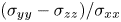 $(\sigma _{yy} - \sigma _{zz})/\sigma _{xx}$ is largely negative, and is almost zero at the centre and approximately 30 % near the wall. Such differences do not appear to have been reported earlier for fully developed flow through a channel. As discussed later, they provide a stringent test of constitutive equations. Unfortunately, we do not have a simple physical explanation for their occurrence. Silbert et al. (Reference Silbert, Ertaş, Grest, Halsey, Levine and Plimpton2001) observed the normal stress difference of approximately 15 %–20 % in inclined chute flow, but they too did not provide a simple explanation. For rough walls, the trends are similar (figure 7d), except that the values are slightly smaller in magnitude near the wall.
Values of the scaled normal stress  $\tilde {N} \equiv N/(\rho _p g, W)$ are of O(1) for the DEM results (figure 7e). For a fixed value of
  $2\,W/d_p$,
  $\tilde {N}$ decreases as
  $\bar {\phi }$ decreases. The stress tensor is evaluated as the sum of two contributions, one arising from contacts (including collisions), and one arising from streaming (Silbert et al. Reference Silbert, Ertaş, Grest, Halsey, Levine and Plimpton2001). Our calculations show that the latter is small compared with the former. Small changes in
  $\bar {\phi }$ cause much larger changes in
  $\tilde {N}$. For systems with high values of
  $\bar {\phi }$, this may be anticipated as the frictional or contact stresses are known to be sensitive to small changes in
  $\phi$. Further, the material is expected to lose sustained contact with the wall as
  $\bar {\phi }$ decreases. Hence
  $\tilde {N}$ is likely to decrease. As mentioned by one of the referees, the stress depends on both the strength of the contact forces and the number of contacts. If the latter dominates,
  $\tilde {N}$ will decrease as
  $\bar {\phi }$ decreases. However, we do not have a convincing argument to prove this assertion at present. It is hoped that a more satisfactory argument may be advanced in the future. For a fixed value of
  $\bar {\phi }$,
  $\tilde {N}$ is a very weak function of
  $2 W/d_p$. Thus the scaling
  $\tilde {N} = N/(\rho _p g W)$ is reasonable but not exact. The normal stress for the smooth wall is approximately 12 %–20 % higher than that for the rough wall (figure 7e). Intuitively, as the angle of wall friction
  $\delta$ is expected to be higher for the rough wall, (3.35) explains the decrease of
  $\tilde {N}$ with the increase in wall roughness for a fixed value of
  $\bar {\phi }$.
The value of the angle of wall friction  $\delta$, calculated from (3.34) decreases by approximately 50 % of the larger value as
  $\bar {\phi }$ increases, for both smooth and rough walls (see the inset of figure 7e). For a fixed value of
  $\bar {\phi }$,
  $\delta$ is approximately 15 %–20 % higher for rough walls than for smooth walls. Compared with the slip b.c. (3.33), the wall friction b.c. (3.34) appears to be more robust. This issue merits further investigation.
As the shear rate and the shear stress increase with  $x/W$ and the normal stress
  $N$ is a constant, both
  $\mu \equiv \tau /N$ and
  $I$ increase, leading to the behaviour shown in figure 8. For very small values of
  $I$,
$I$,  $\mu$ appears to tend to a non-zero value. For intermediate values of
  $I$, the curves for smooth and rough walls are almost identical except for
  $\bar {\phi } = 0.62$. For large values of
  $I$,
$I$,  $\mu$ is larger for rough walls than for smooth walls (figure 8). As the curves for
  $I$ (figure 6) intersect near the wall, the value of
  $I$ in the wall region is lower for the rough wall . Hence, for a fixed value of
  $I$, the corresponding value of
  $x/W$ is larger for the rough wall, leading to a larger value of
  $\tau$. As the normal stress
  $N$ is also smaller for the rough wall (figure 7e),
  $\mu$ is higher near the wall.

Figure 8. Variation of the friction coefficient  $\mu$ with the inertial number
  $I$. The first row (a–d) and second row (e–h) correspond to
  $2\,W/d_p = 40$ and 80, respectively: (a,e),
  $\bar {\phi } = 0.62$; (b, f),
  $\bar {\phi } = 0.61$; (c,g),
  $\bar {\phi } = 0.60$; (d,h),
  $\bar {\phi } = 0.59$. The markers (
 $\circ$ – smooth walls,
  $\square$ – rough walls) correspond to the DEM results and the curves to the model predictions of Barker et al. (Reference Barker, Schaeffer, Shearer and Gray2017) (brown solid line); Schaeffer et al. (Reference Schaeffer, Barker, Tsuji, Gremaud, Shearer and Gray2019) (red dashed line); Henann & Kamrin (Reference Henann and Kamrin2013) (green dotted line).
As  $I$ increases, the shear rate increases. Hence the material is expected to dilate more leading to a lower value of
  $\phi$, or a higher value of
  $\phi _{drp} - \phi$ (figure 9). Except for
  $\bar {\phi } = 0.62$, the results for smooth and rough walls almost coincide, indicating that
  $\phi$ vs
  $I$ relation is independent of the wall roughness. For
  $\bar {\phi } = 0.62$,
  $\phi$ is slightly lower for rough walls. For
  $2\,W/d_p = 80$, there are two distinct regimes, except for
  $\bar {\phi } = 0.62$, (i) where
  $\phi _{drp} - \phi$ increases gradually with
  $I$, and (ii) where
  $\phi _{drp} - \phi$ increases more rapidly for
  $I > 10^{-1}$.

Figure 9. Variation of  $\phi _{drp} - \phi$ with
  $I$. The first row (a–d) and second row (e–h) correspond to
  $2\,W/d_p =$ 40 and 80, respectively: (a,e),
  $\bar {\phi } = 0.62$; (b, f),
  $\bar {\phi } = 0.61$; (c,g),
  $\bar {\phi } = 0.60$; (d,h),
  $\bar {\phi } = 0.59$. The markers (
 $\circ$ – smooth walls,
  $\square$ – rough walls) correspond to the DEM results; Barker et al. (Reference Barker, Schaeffer, Shearer and Gray2017) (brown solid line); Schaeffer et al. (Reference Schaeffer, Barker, Tsuji, Gremaud, Shearer and Gray2019) (red dashed line).
4.2. Barker et al. (Reference Barker, Schaeffer, Shearer and Gray2017)
For reasons explained in § 4.2.1, this model could not be solved for the entire range of parameter values used here. Using (3.23), (3.25), (3.27) and (3.31),  $\phi$,
  $I$ and
  $N$ can be obtained independently of the wall roughness. This result is a consequence of matching
  $\bar {\phi }$ to the DEM results, and not using the alternative b.c. (3.34). Hence the velocity gradient (3.30) is the same for both smooth and rough walls, and the velocity profile corresponds to a shift along the velocity axis when the wall roughness changes. Thus the form of the velocity profile in unaffected by the wall roughness, as shown in figure 3(c,d) (the brown curves). The same conclusion holds for the model of Schaeffer et al. (Reference Schaeffer, Barker, Tsuji, Gremaud, Shearer and Gray2019).
For  $2\,W/d_p = 40$, the magnitude of the scaled velocity is qualitatively similar to the DEM results (the brown curves in figure 3c,d). The values are underestimated near the centre and overestimated near the wall for both smooth and rough walls.
For  $2\,W/d_p = 80$ and
  $\bar {\phi } = 0.62$, the profile agrees fairly well with the DEM results for smooth walls (the brown curve in figure 3e). However, the values are overestimated near the centre and underestimated near the wall for
  $\bar {\phi } = 0.61$ and smooth walls, unlike the case for
  $2\,W/d_p = 40$ (the brown curve in figure 3f). For rough walls, the scaled velocity changes sign near the wall because of the shift, and hence leads to unrealistic profiles (not shown in figure 3e, f).
The scaled thickness of the shear layer  $\varDelta /d_p$ varies with
  $\bar {\phi }$ and
  $2\,W/d_p$ like the DEM results (the brown symbols in figure 4b). It is of the same order of magnitude, but the range is larger than the latter. For reasons explained earlier, this model predicts that
  $\varDelta /d_p$ is independent of the wall roughness, in contrast to the DEM results.
The values of the slip length  $l_u$ calculated from (3.33) vary widely (the brown symbols in figure 4d). In some cases, they exceed the half-width of the channel. Thus this b.c. is not reasonable for this model. Conversely, if
  $l_u$ is treated as a material parameter, the predicted mass flow rates will differ significantly from the DEM results.
The solids fraction profiles are approximately flat, as shown by the insets of figure 5(c–f) (the brown curves). It behaves like an incompressible model, at least in the present problem, and hence does not match the DEM results well. As discussed earlier, the profiles are independent of the wall roughness for a fixed value of  $\bar {\phi }$.
The vertical asymptotes in the  $I$ profiles correspond to the boundary between the plug and the shear layers (the brown curves in figure 6c–f), whereas the DEM results show a more gradual variation. The profiles agree reasonably well with the latter near the wall.
The scaled shear stress  $\tilde {\tau }$ almost coincides with the DEM results for all the models, and hence the profiles are not shown. The first normal stress difference
  $\sigma _{xx} - \sigma _{yy}$ is zero, and the second normal stress difference
  $\sigma _{yy} - \sigma _{zz}$ cannot be evaluated as
  $\sigma _{zz}$ is unknown. This is at variance with the DEM results, particularly near the wall (figure 7c,d). The scaled normal stress
  $\tilde {N} = N/(\rho _p g W)$ underestimates the DEM results, and is independent of wall roughness as mentioned earlier (the brown symbols in figure 7e). Unlike the latter,
  $\tilde {N}$ varies more strongly with
  $2\,W/d_p$ and
  $\bar {\phi }$.
Hence the angle of wall friction  $\delta$ cannot be treated as a material parameter (see (3.35)). Further, as
  $\tilde {N}$ is independent of wall roughness, the model predicts that
  $\delta$ is also independent of the wall roughness, contrary to expectation. This problem arises because
  $\bar {\phi }$ has been matched to the DEM value. On the other hand, if
  $\delta$ is determined from independent experiments, then the predicted value of
  $\bar {\phi }$ for a fixed value of
  $2\,W/d_p$ may not match the value used to generate the DEM results.
From (3.26), as  $I \rightarrow 0$,
  $\mu \rightarrow \mu _s = 0.38$, which is much larger than the DEM results (the brown curves in figure 8c–f). At large values of
  $I$, the trends are similar to the DEM results for rough walls, but the values of
  $\mu$ are overestimated. For smooth walls, the latter show a different curvature. Thus a single function
  $\mu (I)$ cannot fit data for both smooth and rough walls. The brown curves in figure 8(c–f) are obtained by fitting (3.26) to the DEM results of Chialvo et al. (Reference Chialvo, Sun and Sundaresan2012) for homogeneous shear between parallel plates (figure 2a). As this function does not fit our DEM results well, it follows that
  $\mu (I)$ is not a true constitutive equation, but one that depends on the geometry. As
  $\phi$ does not vary much with
  $x/W$ (the insets in figure 5c–f), plots of
  $\phi$ vs
  $I$ are effectively horizontal lines, and hence they do not capture the variation shown by the DEM results (the brown curves in figure 9).
4.2.1. Reasons for the lack of solutions for some parameter values
Introducing the dimensionless quantities  $\tilde {x}_p \equiv x_p/W$ and
  $\tilde {N} \equiv N/(\rho _p g W)$, (3.29) reduces to
  $\tilde {x}_p = (\mu _s \tilde {N})/ \phi _p$. As
  $\tilde {x}_p \leqslant 1$, we have
 \begin{equation} \mu_s\tilde{N} \leqslant \phi_p . \end{equation}
As  $\beta (I \rightarrow 0) = 2\,\mu _s$, (3.27) implies that
 \begin{equation} \phi_p = \frac{\mu_s \tilde{\varLambda}\phi_{min} + \tilde{N}\phi_{max}}{\mu_s \tilde{\varLambda} + \tilde{N}} , \end{equation}
where  $\tilde {\varLambda } \equiv \varLambda /(\rho _p gW)$. Using (4.1) and (4.2), we obtain
 \begin{equation} \mu_s \tilde{N}^{2} + (\mu_s^{2}\tilde{\varLambda} - \phi_{max})\tilde{N} - \mu_s\tilde{\varLambda}\phi_{min} \leqslant 0. \end{equation}
For (4.3) to hold,  $\tilde {N}$ must be less than a critical value
  $\tilde {N}_c$, which is the positive root obtained by equating the left-hand side of (4.3) to zero. For a chosen value of
  $\tilde {\varLambda }$, the root corresponds to the point of intersection of the curve (4.2) and the line given by equality in (4.1) in the
  $\phi _p$–
 $\tilde {N}$ plane (figure 10). For a value of
  $2\,W/d_p$, or
  $\tilde {\varLambda }$, if the curve (4.2) corresponding to that
  $\tilde {\varLambda }$ crosses the line (4.1) at a
  $\phi _p = \phi _{u}$, the model cannot be solved for
  $\bar {\phi } > \phi _{u}$.

Figure 10. Variation of the dimensionless normal stress  $\tilde {N}$ with the solids fraction
  $\phi _p$ in the plug layer for the model of Barker et al. (Reference Barker, Schaeffer, Shearer and Gray2017): solid curves, plots of (4.2) for specified values of
  $\tilde {\varLambda } = \varLambda /(\rho _p g W)$, where
  $\rho _p$ is the particle density,
  $g$ is the acceleration due to gravity and
  $W$ is the half-width of the channel in the
  $x$-direction; upper dash-dot line, equality in (4.1); lower dashed line, equality in (4.6).
An approximate solution provides an additional insight. As seen from our DEM results, the model predicts a very small variation of  $\phi$ (the insets in figure 5c–f). Treating
  $\phi$ as a constant (
 ${=}\phi _p$), and using (3.25) and (3.26), the second of (3.23) can be integrated to obtain
 \begin{equation} \frac{I}{I_0+I} = \frac{\phi_p}{\tilde{N} \Delta \mu} (\tilde{x}-\tilde{x}_p) , \end{equation}
where  $\tilde {x} \equiv x/W$ and
  $\tilde {x}_p \equiv x_p/W$. Simplifying, we obtain
 \begin{equation} I = \frac{I_0 (\tilde{x} - \tilde{x}_p)}{\left(\dfrac{\tilde{N} \mu_d}{\phi_p} - \tilde{x} \right)} ; \quad \mu_d \equiv \mu_s + \Delta \mu . \end{equation}
Equation (4.5a,b) shows that  $I \rightarrow \infty$ as
  $\tilde {x}$ increases if
 \begin{equation} \frac{\tilde{N} \mu_d}{\phi_p} \leqslant 1. \end{equation}
For a chosen value of  $\tilde {\varLambda }$, the limiting condition corresponds to the intersection of the curve (4.2) with the line given by the equality in (4.6) (figure 10). This gives a limiting value of
  $\phi _p = \phi _l$ such that there is no solution for
  $\bar {\phi } < \phi _l$. Thus the model cannot be solved for both small and large values of
  $\bar {\phi }$, but the limits depend on the value of
  $\tilde {\varLambda }$. The lower limit should be used with care as it is based on an approximate solution.
For typical values of a particle density  $\rho _p = 2650\ \textrm {kg}\ \textrm {m}^{-3}$,
  $\varLambda = 555 \ \textrm {N}\ \textrm {m}^{-2}$, a particle diameter
  $d_p = 1$ mm and
  $2\, W/d_p = 30$, 40, 50 and 80, the values of
  $\tilde {\varLambda } = \varLambda /(\rho _p g W)$ are 1.4, 1.1, 0.8 and 0.5, respectively. For these values of
  $\tilde {\varLambda }$, figure 10 shows that solutions can be obtained for
  $\bar {\phi } = (0.6, 0.59)$ for
  $2\,W/d_p = 30$ and 40, (0.61, 0.6, 0.59) for
  $2\,W/d_p = 50$ and (0.62, 0.61) for
  $2\,W/d_p = 80$.
4.3. Schaeffer et al. (Reference Schaeffer, Barker, Tsuji, Gremaud, Shearer and Gray2019)
As  $\bar {\phi }$ is matched to the DEM results and
  $\phi _c = 0.613$ in (3.40), a solution could not be obtained for
  $\bar {\phi } = 0.62$. As
  $\phi (x = 0) \approx 0.63$ for the DEM results and
  $\phi (x = 0) \leqslant \phi _c$ for the model, we expect the predictions to overestimate
  $\phi$ near the wall for
  $\bar {\phi } \leqslant 0.61$ (the red curves in figure 5). The scaled velocity profiles are qualitatively similar to the DEM results, except that the values are higher near the wall and lower near the centre (the red curves in figure 3). This holds for both smooth and rough walls. The scaled thickness of the shear layer
  $\varDelta /d_p$ overestimates the DEM results for most of the parameter values (the red symbols in figure 4b), but is of the same order of magnitude. It varies with
  $2\,W/d_p$ and
  $\bar {\phi }$, but does not vary with the wall roughness, similar to that of Barker et al. (Reference Barker, Schaeffer, Shearer and Gray2017). The range of
  $l_u/d_p$ values is comparable to that of Barker et al. (Reference Barker, Schaeffer, Shearer and Gray2017) (the red symbols in figure 4d). As in the case of the latter,
  $l_u$ is not a material parameter.
The  $\phi$ profiles (the red curves in figure 5) are better than the flat profiles predicted by Barker et al. (Reference Barker, Schaeffer, Shearer and Gray2017). However, there is no improvement in the profiles of
  $I$, which are similar to those of Barker et al. (Reference Barker, Schaeffer, Shearer and Gray2017), except near the wall (the red curves in figure 6). For a fixed value of
  $\bar {\phi }$, the
  $I$ profiles are independent of
  $2\,W/d_p$ unlike the profiles of Barker et al. (Reference Barker, Schaeffer, Shearer and Gray2017). This is because the right-hand side of (3.41) involves the ratio of
  $x/W$ to the scaled normal stress
  $\tilde {N} = N/(\rho _p g W)$, and
  $W$ does not occur explicitly. Hence
  $\phi$ is independent of
  $2\,W/d_p$ (see (3.40)), leading to a similar behaviour for
  $\tilde {N}$ (the red symbols in figure 7e). Equation (3.35) shows that
  $\delta$ is also independent of
  $2\,W/d_p$, and varies only with
  $\bar {\phi }$. The values
  $\tilde {N}$ are underestimated. The first normal stress difference is zero, and the second normal stress difference is undetermined. As explained in § 4.2, the profiles of
  $\phi$,
  $I$, and
  $\tilde {N}$ are unaffected by the wall roughness, and hence the remarks about the use of the friction b.c. (3.35) apply here also.
The profiles of  $\mu$ vs
  $I$ are identical to those of Barker et al. (Reference Barker, Schaeffer, Shearer and Gray2017), as (3.26) has been used in both cases (the red curves in figure 8). For
  $I$ in the range 0.002–0.2, (3.40) has been fitted to the DEM results. Hence the agreement is good (the red curves in figure 9). For smaller values of
  $I$, deviations are apparent.
4.4. Henann & Kamrin (Reference Henann and Kamrin2013)
For smooth walls, the scaled velocity profiles are qualitatively similar to those for the DEM results (the green curves in figure 3), but the values are underestimated near the centre and overestimated near the wall. For rough walls, the solution could not be obtained as discussed in § 4.4.1. For smooth walls, the scaled thickness of the shear layer is comparable to the DEM results (the green symbols in figure 4b).
The value of the slip length  $l_u$ is approximately independent of
  $\bar {\phi }$ and
  $2\,W/d_p$, and comparable to the DEM results (the green symbols in figure 4d). Hence it appears that the slip velocity b.c. (3.33) can be used for this model, with
  $l_u$ as a material parameter.
The slip length for the fluidity  $l_f$ is calculated using (3.58), and is shown in figure 11(a). The DEM results of
  $l_f$ for smooth walls do not vary with
  $2\,W/d_p$ and
  $\bar {\phi }$, which is not true for rough walls. For smooth walls, the value of
  $l_f$ obtained from the model is much smaller than that for the DEM results, and shows a very weak dependence on
  $2\,W/d_p$ and
  $\bar {\phi }$. Thus (3.58) can possibly be used as a b.c., but the discrepancy in the
  $l_f$ values shown in figure 11(a) suggests that it may not give good predictions of various quantities.

Figure 11. Variation of  $l_f$ (a) and
  $\tilde {x}_s = \mu _s \tilde {N}/\phi _p$ (b) with
  $\bar {\phi }$,
  $\tilde {f} = f/f_w$ (c) and
  $T_1$ and
  $T_2$ (d) with
  $\tilde {x} = x/W$ for the model of Henann & Kamrin (Reference Henann and Kamrin2013). Here,
  $l_f$ is calculated from (3.58),
  $T_1$ and
  $T_2$ are defined by (4.9a,b). The value of
  $\tilde {N}$ is matched to the DEM results. In (a,b), open and filled symbols correspond to smooth and rough walls, and
  $\vartriangle$,
  $\diamond$,
  $\circ$, and
  $\square$ are for
  $2\,W/d_p = 30$, 40, 50 and 80, respectively. In (a), the solid lines correspond to the DEM results, and the dotted lines to the model predictions. In (c,d),
  $2\,W/d_p = 40$; black dash-dotted line,
  $\bar {\phi } = 0.62$ (smooth wall,
  $\tilde {x}_s > 1$); black solid line,
  $\bar {\phi } = 0.6$ (smooth wall,
  $\tilde {x}_s$ slightly
  $<$ 1); black dashed line,
  $\bar {\phi } = 0.6$ (rough wall,
  $\tilde {x}_s$ much
  $<1$). The numerical (blue) and approximate (red) solutions for
  $\tilde {f}$ are shown in (c). Using the numerical solution, the profiles of
  $T_1$ (black) and
  $T_2$ (magenta) are shown in (d).
As  $\phi$ is assumed to be a constant, the profiles are flat, in contrast to the DEM results (the green curves in figure 5). The variation of
  $I$ with
  $x/W$ is predicted fairly well by the model (the green curves in figure 6). The normal stress differences are zero (see (3.44)), in contrast to the DEM results. The scaled normal stress
  $\tilde {N}$ has been matched to the DEM values, and hence there is no discrepancy in the values of
  $\tilde {N}$ and
  $\delta$. Conversely, if the value
  $\delta$ is taken from independent experiments, the predicted value of
  $\tilde {N}$ may not match the DEM results. For smooth walls,
  $\mu$ vs
  $I$ profiles are predicted much better than the other models (the green curves in figure 8). In particular, the change in curvature of the profiles near the wall for some of the parameter values is captured by the model. Solutions could not be obtained for some parameter values (e.g. for rough walls), for reasons discussed below.
4.4.1. Reasons for the lack of solutions
Introducing the dimensionless variables  $\tilde {x} = x/W$,
  $\tilde {W} = W/d_p$,
  $\tilde {u}_y = u_y/\sqrt {g W}$,
  $\tilde {N} = N/(\rho _p g W)$,
  $\tilde {f} = f/f_{w}$,
  $\tilde {f}_{w} = f_{w}/\sqrt {g/W}$, where
  $f_w = f(x = W)$, and substituting
  $\mu$ from (3.52), (3.53) can be rewritten as
 \begin{equation} \frac{ \mbox{d}^{2} \tilde{f}}{ \mbox{d} \tilde{x}^{2}} = \frac{\Delta \mu}{A^{2}} \left( \frac{\tilde{x}_s - \tilde{x}}{\tilde{x}_d - \tilde{x}} \right) \tilde{W}^{2} \tilde{f} + \frac{\Delta \mu}{I_0 A^{2}} \, \frac{\phi_p}{\tilde{N}^{3/2}} \tilde{W} \tilde{f}_{w} \tilde{x} \tilde{f}^{2} ,\end{equation}
or
 \begin{equation} \frac{ \mbox{d}^{2} \tilde{f}}{ \mbox{d} \tilde{x}^{2}} = T_1 + T_2 , \end{equation}
where  $\tilde {x}_s \equiv \mu _s \tilde {N}/\phi _p$ and
  $\tilde {x}_d \equiv (\mu _s + \Delta \mu ) \tilde {N} / \phi _p$, and
 \begin{equation} T_1 \equiv \frac{\Delta \mu}{A^{2}} \left( \frac{\tilde{x}_s - \tilde{x}}{\tilde{x}_d - \tilde{x}} \right) \tilde{W}^{2} \tilde{f}; \quad T_2 \equiv \frac{\Delta \mu}{I_0 A^{2}} \, \frac{\phi_p}{\tilde{N}^{3/2}} \, \tilde{W} \tilde{f}_{w} \tilde{x} \tilde{f}^{2} .\end{equation}
The values of  $\mu _s$ and
  $\Delta \mu$ are such that
  $\tilde {x}_d > \tilde {x}_s$ and
  $\tilde {x}_d > 1$ for the ranges of
  $\tilde {N}$ and
  $\phi _p (= \bar {\phi })$ used here. However,
  $\tilde {x}_s$ may be
  $> 1$ for some cases (figure 11b). If
  $\tilde {x}_s > 1$, the right-hand side of (4.7) is non-negative. Using the b.c. (3.56), if
  $\tilde {f}(\tilde {x} = 0) > 0$, then (4.7) implies that
  $\tilde {f}$ increases monotonically throughout the domain. Hence a solution can be obtained that matches the b.c. (3.57) for smooth walls (the blue dash-dot curve in figure 11c).
If  $\tilde {x}_s$ is slightly
  ${<} 1$,
  $T_1$ is
  ${<}0$ near the wall, whereas
  $T_2$ is
  ${>}0$ (see (4.9a,b)). If the latter dominates, a solution can be obtained (the solid blue curve in figure 11c). If
  $\tilde {x}_s$ is much
  ${<}1$,
  $T_1$ is
  ${<}0$ for
  $\tilde {x}_s < \tilde {x} \leqslant 1$, and may dominate
  $T_2$ in magnitude. Hence the right-hand side of (4.7) may be negative for some values of
  $\tilde {x}$. This causes the slope
  $\mbox {d} \tilde {f}/\mbox {d} x$ to decrease. If the slope decreases,
  $\tilde {f}$ may eventually become
  $< 0$, as in the case of the blue dashed curve in figure 11(c). This is an unrealistic result as (3.45) implies that
  $\tilde {f}$ must be
  $\geqslant 0$. For rough walls,
  $\tilde {x}_s$ is significantly
  ${<}1$ (figure 11b), and hence a realistic solution could not be obtained.
4.4.2. An approximate solution by the method of matched asymptotic expansion
An insight into the behaviour of solutions to (4.7) may be obtained by omitting  $T_2$ as discussed below, even though the numerical solution shows that
  $|T_1| \ll T_2$ near the wall (figure 11d). Introducing a small parameter
  $\varepsilon = 1/\tilde {W} = d_p/W$,
  $\tilde {f}$ may be expanded in powers of
  $\varepsilon$ as
 \begin{equation} \tilde{f} = \tilde{f}_0 (\tilde{x}) + \varepsilon \tilde{f}_1(\tilde{x}) + \varepsilon^{2} \tilde{f}_2 (\tilde{x}) + \dots . \end{equation}
Substituting (4.10) in (4.7), omitting  $T_2$ and matching the terms of
  ${O}$(
 $\varepsilon ^{0}$), we obtain
  $\tilde {f}_0 = 0$. This does not satisfy the b.c. (3.57) at
  $\tilde {x} = 1$. Regarding this as the outer solution
  $\tilde {f}_{outer} = 0$ which is not valid near the wall, we seek an inner solution
  $\tilde {f}_{inner}$ by introducing a new coordinate
 \begin{equation} X = (1 - \tilde{x})/\varepsilon . \end{equation}
Expanding  $\tilde {f} = \tilde {f}_{inner} \equiv F$ in powers of
  $\varepsilon$, we obtain
 \begin{equation} F = F_0 (X) + \varepsilon F_1 (X) + \varepsilon^{2} F_2 (X) + \dots.\end{equation}
Substituting (4.11) and (4.12) in (4.7), we obtain
 \begin{equation} \frac{ \mbox{d}^{2} F}{ \mbox{d} X^{2}} = \frac{\Delta \mu}{A^{2}} \, \frac{\tilde{x}_s - (1-\varepsilon X)}{\tilde{x}_d - (1-\varepsilon X)} \, F . \end{equation}
The b.c.s required to solve (4.13) are  $F (X = 0) = 1$ and
  $F \rightarrow \tilde {f}_{outer} = 0$ as
  $X \rightarrow \infty$. Substituting (4.12) in (4.13), and matching the terms of O(
 $\varepsilon ^{0}$), we obtain
 \begin{equation} \frac{ \mbox{d}^{2} F_0}{ \mbox{d} X^{2}} = m^{2} F_0 ,\end{equation}
where  $m^{2} = (\Delta \mu /A^{2}) ((\tilde {x}_s - 1)/(\tilde {x}_d - 1))$, and the leading-order terms in the b.c. are
  $F_0 (X = 0) = 1$ and
  $F_0 \rightarrow \tilde {f}_{outer}$ as
  $X \rightarrow \infty$.
Case 1: for  $\tilde {x}_s > 1$,
  $m^{2}$ is
  $> 0$ and the inner solution is
 \begin{equation} \tilde{f}_{inner} = F = F_0 + {O}(\varepsilon) = \exp ({-}m X) + {O}(\varepsilon) = \exp \left( -\frac{m}{\varepsilon} (1-\tilde{x}) \right) + {O} (\varepsilon), \end{equation}
which ensures the solution  $\tilde {f}$ is
  $\geqslant 0$ in the whole domain. The exponentially decaying trend of (4.15) from the wall towards the centre agrees qualitatively with the numerical results (the blue dash-dot curve and the blue solid curve in figure 11c).
Case 2: for  $\tilde {x}_s < 1$,
  $m^{2}$ is
  $< 0$ and the inner solution is
 \begin{equation} \tilde{f}_{inner} = F (X) = F_0 (X) + {O} (\varepsilon) = c_1 \cos (m X) + c_2 \sin (m X) + {O}(\varepsilon) ,\end{equation}
where  $c_1$ and
  $c_2$ are constants. Using the b.c.
  $F_0(X = 0) = 1$,
  $c_1 = 1$. The b.c.
  $F_0 \rightarrow \tilde {f}_{outer}$ as
  $X \rightarrow \infty$ cannot be satisfied. Hence the solution (4.16) does not ensure
  $\tilde {f} \geqslant 0$ in the whole domain for the instances
  $\tilde {x}_s < 1$.
The above argument very crudely suggests that there is a possibility of obtaining a solution with  $\tilde {f} < 0$ in a part of the domain if
  $|T_1| > T_2$. The numerical solution shows that
  $T_2$ is
  ${\gg }|T_1|$ near the wall, although both the terms are comparable in a zone far from the wall (figure 11d). This leads us to seek an approximate solution by omitting
  $T_1$.
Introducing a small parameter  $\epsilon _* = 1/(\tilde {W} \tilde {f}_w)^{1/2}$ (the DEM results show that
  $\tilde {f}_w$ is of the same order as
  $\tilde {W}$), (4.7) can be rewritten as
 \begin{equation} \frac{ \mbox{d}^{2} \tilde{f}}{ \mbox{d} \tilde{x}^{2}} = \epsilon_*^{2} \frac{\Delta \mu}{I_0 A^{2}} \, \frac{\phi_p}{\tilde{N}^{3/2}} \, \tilde{x} \tilde{f}^{2} . \end{equation}
Expanding  $\tilde {f}$ in powers of
  $\epsilon _*$
 \begin{equation} \tilde{f} = \tilde{f}_0 + \epsilon_* \tilde{f}_1 + \epsilon_*^{2} \tilde{f}_2 + \dots . \end{equation}
Substituting (4.18) in (4.17), and matching the terms of O( $\epsilon _*^{0}$), we obtain
 \begin{equation} \tilde{f}_0 = 0 . \end{equation}
The solution (4.19) satisfies the b.c.  $\mbox {d} \tilde {f}/\mbox {d} \tilde {x} (\tilde {x} = 0) = 0$, but not the b.c.
  $\tilde {f} (\tilde {x} = 1) = 1$. Hence we regard (4.19) as the outer solution
  $\tilde {f}_{outer}$.
To obtain the inner solution, let
 \begin{equation} \chi = \frac{1 - \tilde{x}}{\epsilon_*} . \end{equation}
Expanding  $\tilde {f} = \tilde {f}_{inner} \equiv \varphi$ in powers of
  $\epsilon _*$, we obtain
 \begin{equation} \varphi = \varphi_0 (\chi) + \epsilon_* \varphi_1 (\chi) + \epsilon_*^{2} \varphi_2 (\chi) + \dots . \end{equation}
Substituting (4.21) in (4.17), we obtain
 \begin{equation} \frac{ \mbox{d}^{2} \varphi}{ \mbox{d} \chi^{2}} = \frac{\Delta \mu}{I_0 A^{2}} \, \frac{\phi_p}{\tilde{N}^{3/2}} (1 - \epsilon_* \chi) \varphi^{2} . \end{equation}
The b.c.s for (4.22) are  $\varphi (\chi = 0) = 1$ and
  $\varphi \rightarrow \tilde {f}_{outer} = 0$ as
  $\chi \rightarrow \infty$. Substituting (4.21) in (4.22), and matching the terms of O(
 $\epsilon _*^{0}$), we obtain
 \begin{equation} \frac{ \mbox{d}^{2} \varphi_0}{ \mbox{d} \chi^{2}} = \alpha \varphi_0^{2} , \end{equation}
where  $\alpha = (\Delta \mu \phi _p)/(I_0 A^{2} \tilde {N}^{3/2})$. Multiplying both sides of (4.23) by
  $\mbox {d} \varphi _0 / \mbox {d} \chi$, and using the b.c.s
  $\varphi _0 (\chi = 1) = 1$ and
  $\varphi _0 \rightarrow 0$ at
  $\chi \rightarrow \infty$, the inner solution is given by (Zaitsev & Polyanin Reference Zaitsev and Polyanin2002)
 \begin{equation} \tilde{f}_{inner} = \varphi = \frac{1}{\left( \sqrt{\dfrac{\alpha}{6}} \chi + 1 \right)^{2}} + {O}(\epsilon_*) . \end{equation}
The approximate solution (the red curves in figure 11c) agrees reasonably well with the numerical solution (the blue curves), except when the fluidity is negative.
4.4.3. Use of  $\phi = \phi (I)$ to improve the model

To permit variation of  $\phi$ with
  $x$, we assume that
  $\phi = \phi (I)$, and use the form (3.40). Equations (3.30), (3.50a,b) and (3.53) are solved using the b.c.s (3.56) and (3.57). As in the other models,
  $\bar {\phi }$ and
  $\dot {M}$ are matched to the DEM results. For
  $\bar {\phi } = 0.61$, the
  $\phi$ profiles (the blue and red solid curves in figure 12b) agree better with the DEM results than the incompressible model (the dashed line). Because
  $\phi (x = 0) = \phi _c = 0.613$ at the centre, which is slightly
  ${>}\phi _p = \bar {\phi }$ for the incompressible model, we expect the scaled velocity to be smaller near the centre (the blue and red solid curves in figure 12a). The profiles of
  $I$ for both the models are qualitatively similar (figure 12c). These remarks also apply to the case
  $\bar {\phi } = 0.60$ (figure 12d–f).

Figure 12. Variation of the scaled vertical velocity  $-u_y/\sqrt {gW}$ (a), the solids fraction
  $\phi$ (b) and the inertial number
  $I$ (c) with
  $x/W$ for the model of Henann & Kamrin (Reference Henann and Kamrin2013):
  $\circ$, the DEM results; blue and red dashed line,
  $\phi = \textrm {const}. = \phi _p$; blue and red solid line,
  $\phi = \phi (I)$;
  $2\,W/d_p = 40$, red curves;
  $2\,W/d_p = 80$, blue curves. Here,
  $\bar {\phi } = 0.61$ (a–c), and 0.60 (d–f).
4.5. Dsouza & Nott (Reference Dsouza and Nott2020)
The value of the parameter  $\ell$ is estimated by minimizing the root mean square error
  $N_{rms}$ between the normal stresses
  $N_{dem}$ and
  $N_{model}$, with
 \begin{equation} N_{rms} \equiv \sqrt{ \frac{1}{n_p} \sum_{i = 1}^{n_p} \left( \frac{N_{model} - N_{dem}}{N_{dem}} \right)^{2} } , \end{equation}
where  $n_p$ is the number of bins used for the DEM. For the models,
  $N_{model} = \sigma _{xx}$ is independent of
  $x$, but
  $N_{dem}$ varies slightly. Here,
  $N_{rms}$ increases with
  $\ell /d_p$ (figure 13a), and hence there is no obvious choice for
  $\ell /d_p$. Clearly,
  $\ell$ should be small compared with the half-width
  $W$ of the channel and large enough so that the averaging volume used to average the flow rule contains a reasonable number of particles. The smallest value of
  $\ell /d_p$ used here is 3. Choosing a value of
  $N_{rms}$ that is 5 % larger than the value for
  $\ell /d_p = 3$, and averaging the results for
  $2\,W/d_p = 30$, 40 and 50, we obtain
  $\ell /d_p = 5$. A sphere of radius
  $5 \, d_p$ contains
  ${\approx }75$ particles. The value used by Dsouza & Nott (Reference Dsouza and Nott2020) is
  $\ell /d_p = 10$ but the reason behind this choice is not clear. It leads to a larger discrepancy compared with the DEM results (figure 13a). As mentioned in § 3.5, the dimensionless shear rate
  $\tilde {S} = S' \sqrt {W/g}$ is replaced by
  $\tilde {S} + \tilde {\epsilon }$, where
  $\tilde {\epsilon }$ is chosen as
  $10^{-4}$. The results are unaffected for
  $\tilde {\epsilon }$ in the range
  $10^{-6}{-} 10^{-2}$, and the relative error in the results with respect to
  $\tilde {\epsilon } = 10^{-4}$ is in the range
  $10^{-4}\,\%{-} 10^{-2}$ %.

Figure 13. Variation of the root mean square error for the normal stress  $N_{rms}$ (see (4.25)) with
  $\ell /d_p$ (a), solids fraction
  $\phi$ with
  $x/W$ (b) and the lower limit
  $\bar {\phi }_l$ for
  $\bar {\phi }$ with
  $2\,W/d_p$ and
  $\phi ^{0} \equiv \phi (x = 0)$ (c) for the model of Dsouza & Nott (Reference Dsouza and Nott2020). Here,
  $\ell$ is the effective radius of averaging volume (see (3.59)). In (b), the symbols represent the DEM results for smooth (
 $\circ$) and rough (
 $\square$) walls, and the curves represent the numerical solutions based on (3.60) (black dashed line) and (3.61) (black solid line) for
  $2\,W/d_p = 40$ and
  $\bar {\phi } = 0.62$. The scaled normal stresses
  $\tilde {N}$ predicted by (3.60) and (3.61) are 6.26 and 4.16
  $\times 10^{4}$ , respectively. In (c),
  $\bar {\phi }_l$ corresponds to
  $\phi (x = W) = \phi _{min}$ (see (3.60)).
The results are sensitive to the choice of the functional form of  $\varPi (\phi )$, the local value of the mean stress at a critical state. The two forms used here (3.60) and (3.61) lead to very different profiles of
  $\phi$ in the shear layer and also different estimates of the normal stresses (figure 13b). The local contribution of the critical state pressure
  $\varPi (\phi )$ diverges faster for (3.61) than (3.60). The ratio of
  $\varPi (\phi )$ calculated from (3.61) and (3.60) for, say,
  $\phi (x = 0) = 0.63$ is
  ${\approx }10^{3}$, which explains the much higher prediction of the scaled normal stress
  $\tilde {N}$ for (3.61). There is a dire need for data on
  $\varPi (\phi )$ at stress levels comparable to those that occur in laboratory-scale experiments.
Equation (3.64) could not be solved except for  $\bar {\phi } = 0.62$. The reason for this behaviour is discussed in § 4.5.1. As the centreline velocity is forced to match the DEM value, the prediction is good near the centre (the magenta curves in figure 3a,e). However, the DEM results are significantly underestimated except close to the wall. Consequently, the predicted thickness of the shear layer is much higher (the magenta symbols in figure 4b). The value of
  $l_u$ calculated from (3.33) varies from 1 to 20 as
  $2\,W/d_p$ increases from 30 to 80 (figure 4d). Hence (3.33) is not a suitable b.c. For rough walls, the magnitude of the scaled velocity changes sign near the wall, which is unrealistic. The reason for this behaviour is discussed in § 4.2.
For smooth walls, the  $\phi$ profiles agree well with the DEM results (the magenta curves in figure 5a,e). For rough walls, discrepancies are evident for intermediate values of
  $x/W$. For a fixed value of
  $\bar {\phi }$,
  $\phi$ profiles depend on
  $\phi (x = 0)$, which is matched to the DEM results. As
  $\phi (0)$ is found to be insensitive to the wall roughness (figure 5a,e), the predicted
  $\phi$ profiles are independent of the wall roughness, in contrast to the DEM results.
The normal stress differences are zero (the first of (3.62)). The scaled normal stress  $\tilde {N}$ is much higher than the DEM results (the magenta symbols in figure 7e). The local model, obtained by setting
  $\ell = 0$ in (3.62)–(3.64), implies that the momentum balance (3.64) cannot be satisfied, and hence it does not predict the variation of
  $\phi$ in the current geometry. However, the local contribution to the normal stress may be readily evaluated using the values of
  $\phi$. For example, if
  $2\,W/d_p = 40$ and
  $\bar {\phi } = 0.61$,
  $\tilde {N}_{local}/\tilde {N} \approx 0.25$ at
  $x = 0$. Thus large normal stresses arise mainly from the non-local term involving
  $\ell ^{2}$ in the first of (3.64). As
  $2\,W/d_p$ increases,
  $\tilde {N}$ decreases, in contrast to the behaviour of the DEM and the other models. Some insight can be gained from an approximate solution discussed in § 4.5.2.
4.5.1. Reasons for the lack of solutions for $\bar {\phi } = 0.59 - 0.61$

The integration of the first of (3.64) from  $x/W = 0$ stops when
  $\phi = \phi _{min}$ for
  $x/W \leqslant 1$. This is because
  $\varPi = 0$ for
  $\phi < \phi _{min}$ (see (3.60)), and hence the normal stress
  $N$ vanishes (see the first of (3.64)). Thus there is a lower limit
  $\bar {\phi } \equiv \bar {\phi }_l$ such that
  $\phi ( x = W) = \phi _{min}$. To obtain
  $\bar {\phi }_l$, we integrate the first of (3.64) using
  $\phi (x = 0) = \phi ^{0}$ and
  $\mbox {d}\phi /\mbox {d}x (x= 0) = 0$, and iterate the value of
  $N$ such that
  $\phi (x = W) = \phi _{min}$. Curves of constant
  $\phi ^{0}$ are shown in figure 13(c). For fixed values of
  $2\,W/d_p$ and
  $\phi ^{0}$, solutions can be obtained for
  $\bar {\phi } > \bar {\phi }_l$. Our DEM results predict
  $\phi ^{0} \approx 0.63$, which is one of the b.c. used to solve the first of (3.64). The curve corresponding to this value shows that solutions cannot be obtained for
  $\bar {\phi } \leqslant 0.61$ (figure 13c).
4.5.2. Approximate solution
The structure of (3.64) and the b.c. permits the construction of a Taylor series solution. Expanding  $\phi$ in a Taylor series about
  $x = 0$, and using the symmetry condition
  $\mbox {d}\phi /\mbox {d}x (x = 0) = 0$
 \begin{equation} \phi = \phi^{0} + \left.\frac{1}{2} \,\frac{\mbox{d}^{2}\phi}{\mbox{d}\kern0.7pt x^{2}} \right|_0 \; x^{2} + {{O}}(x^{4}) . \end{equation}
Using the first of (3.64)
 \begin{equation} \left.\frac{\mbox{d}^{2}\phi}{\mbox{d}\kern0.7pt x^{2}} \right|_0 = \left.\frac{\varPi - N}{\ell^{2} \, \dfrac{\mbox{d}\varPi}{\mbox{d}\phi}} \right|_0 . \end{equation}
Integrating (4.26) with respect to  $x$ from 0 to
  $W$, we obtain
 \begin{equation} \bar{\phi} = \phi^{0} + \left.\frac{1}{6} \, \frac{\mbox{d}^{2}\phi}{\mbox{d}\kern0.7pt x^{2}} \right|_0 W^{2} . \end{equation}
Using (4.26) and (4.28), the approximate solution for  $\phi$ is
 \begin{equation} \phi = \phi^{0} + 3 \left(\bar{\phi} - \phi^{0} \right) \left(\frac{x}{W} \right)^{2} . \end{equation}
To obtain the normal stress  $N$, we use (4.27) and (4.28)
 \begin{equation} N = \varPi_{\phi = \phi^{0}} - 6 \left(\frac{\ell}{W}\right)^{2} \left(\bar{\phi} - \phi^{0} \right) \left.\frac{\mbox{d}\varPi}{\mbox{d}\phi} \right|_{\phi = \phi^{0}} . \end{equation}
Setting  $q = \mbox {d}u_y/\mbox {d}x$, (3.67) reduces to
 \begin{equation} \frac{ \mu_*}{q} \left( N q - \ell^{2} \varPi \left.\frac{\mbox{d}^{2} q}{\mbox{d} x^{2}} \right) \right\vert_x = \rho_p g \int_{0}^{x} \phi \, \mbox{d}\kern0.7pt x' . \end{equation}
Expanding  $q$ in a Taylor series about
  $x = 0$, and using the conditions
  $q(x = 0) = 0$ and
  $\mbox {d}^{2}q/\mbox {d}x^{2}(x = 0) = 0$ (see (3.66))
 \begin{equation} \frac{\mbox{d}u_y}{\mbox{d}\kern0.7pt x} = q = \left.\frac{\mbox{d}q}{\mbox{d}\kern0.7pt x}\right|_0 x + \frac{1}{3!} \left. \frac{\mbox{d}^{3} q}{\mbox{d} x^{3}}\right|_0 x^{3} + {{O}} (x^{5}) . \end{equation}
Now, applying limit  $x \rightarrow 0$ to (4.31), L’Hopital's rule implies that
 \begin{equation} \frac{N \left.\dfrac{\mbox{d} q}{\mbox{d} x} \right|_0 - \ell^{2} \varPi_{\phi = \phi^{0}} \left.\dfrac{\mbox{d}^{3} q}{\mbox{d} x^{3}}\right|_0}{\left.\dfrac{\mbox{d} q}{\mbox{d} x} \right|_0} = 0 . \end{equation}
Assuming that  ${\mbox {d} q}/{\mbox {d} x} |_0 \neq 0$, (4.33) reduces to
 \begin{equation} N \left. \frac{\mbox{d} q}{\mbox{d} x} \right|_0 - \ell^{2} \varPi_{\phi = \phi^{0}}\left. \frac{\mbox{d}^{3} q}{\mbox{d} x^{3}}\right|_0 = 0 . \end{equation}
Solving for  ${\mbox {d}^{3} q}/{\mbox {d} x^{3}}|_0$ from (4.34), integrating (4.32) and using
  $u_y (x = 0) \equiv u_y^{0}$, we obtain
 \begin{equation} u_y = u_y^{0} + \left( \frac{1}{2} x^{2} + \frac{1}{24\ell^{2}} \, \frac{N}{\varPi_{\phi = \phi^{0}}} x^{4} \right) \left. \frac{\mbox{d} q}{\mbox{d} x} \right|_0 . \end{equation}
Using (3.32), (4.29) and (4.35), we obtain
 \begin{equation} \left.\frac{\mbox{d} q}{\mbox{d} x} \right|_0 = \frac{ \left(2 \rho_p B ({-}u_y^{0}) \bar{\phi}W \right) - \dot{M}}{2 \rho_p B \left( \dfrac{3}{10}\bar{\phi}W^{3} + \dfrac{1}{56\ell^{2}} \dfrac{N}{\varPi_{\phi = \phi^{0}}} \bar{\phi} W^{5} + \dfrac{1}{60} \phi^{0} W^{3} - \dfrac{1}{105\ell^{2}} \dfrac{N}{\varPi_{\phi = \phi^{0}}} \phi^{0} W^{5}\right)} . \end{equation}
 The functions (4.29), (4.30), (4.35) and (4.36) provide an approximate solution. The approximate solution for the velocity is close to the numerical solution, except near the wall (figure 3a,e). Owing to the Taylor series expansion, the approximate solution can be constructed for  $\bar {\phi } \leqslant 0.62$, whereas the numerical solution cannot be obtained for
  $\bar {\phi } < 0.62$ (see § 4.5.1). For fixed values of
  $\bar {\phi }$ and
  $x/W$, (4.29) shows that
  $\phi (x/W)$ is independent of
  $W$ (the blue curves in figure 5). The numerical solution (the magenta curves in figure 5a,e) reflects this behaviour except very close to the wall. This is in keeping with the trends shown by the DEM results.
In the absence of the non-local term involving  $(\ell /W)^{2}$ in (4.30),
  $N$ is approximately a constant as
  $\phi ^{0}$ does not vary much with changes in
  $\bar {\phi }$ and
  $2\,W/d_p$ for the DEM results. When the non-local term is included, (4.30) shows that
  $N$ increases as
  $W$ decreases provided
  $\bar {\phi } < \phi ^{0}$, in contrast to the DEM results (the blue symbols in figure 7e). The numerical solution (magenta) is close to the approximate solution. The slope
  $\mbox {d} N/\mbox {d} \bar {\phi }$ of (4.30) is negative, in contrast to the DEM results. Thus higher order terms may be required to get a more accurate solution.
5. Discussion
The problem of the gravity flow of granular material through a vertical channel is examined using the DEM and some continuum models for a wide range  $2\,W/d_p = 30{-} 80$ and
  $\bar {\phi } = 0.62{-} 0.59$. In the DEM simulation, there is no exit slot in the channel, and periodic b.c.s are applied in the flow
  $y$- and the vorticity
  $z$-directions. The range of
  $\bar {\phi }$ appears narrow, but is not as earlier work suggests that the material does not flow for
  $\bar {\phi } > 0.62$. There is a lower limit
  $\bar {\phi } = \bar {\phi }_{cr}$ such that steady flow does not occur for
  $\bar {\phi } < \bar {\phi }_{cr}$. For smooth walls with
  $2\,W/d_p = 80$,
  $\bar {\phi }_{cr} = 0.59$. The value of
  $\bar {\phi }_{cr}$ depends on
  $2\,W/d_p$, and ongoing work suggests that it also depends on the wall roughness.
Let us summarize the DEM results first. They predict a plug at the centre and a shear layer near the wall, in accord with experimental observations. The solids fraction  $\phi$ is approximately constant in the plug and reduces significantly in the shear layer because of dilation. The value of
  $\phi \approx 0.63$ in the plug is approximately independent of the width
  $2\,W/d_p$, the bulk solids fraction
  $\bar {\phi }$, and the wall roughness. However, in the shear layer, the profiles of
  $\phi$ vary with
  $\bar {\phi }$ and the wall roughness for a fixed value of
  $2\,W/d_p$. The scaled thickness of the shear layer
  $\varDelta /d_p$ increases with
  $2\,W/d_p$, in accord with the data of Ananda et al. (Reference Ananda, Moka and Nott2008). It increases as
  $\bar {\phi }$ decreases, and varies with the wall roughness. The mass flow rate
  $\dot {M}$ increases as
  $2\,W/d_p$ increases and
  $\bar {\phi }$ decreases. When
  $\bar {\phi }$ decreases,
  $-u_y$ increases more than the corresponding decrease in
  $\phi$ near the wall. Hence
  $\dot {M}$ increases. For smooth walls, the values of
  $\dot {M}$ are higher than those for rough walls, as expected. The slip length
  $l_u/d_p$ is approximately independent of
  $2\,W/d_p$ and
  $\bar {\phi }$, but the values are nearly 4 times higher for smooth walls than those for rough walls. Thus it may be possible to use the slip b.c. (3.33) for solving flow problems. The inertial number
  $I$ varies from very small values near the centre to large values of O(1) near the wall. It increases as
  $\bar {\phi }$ decreases, and the values are higher near the wall for rough walls than those for smooth walls. The normal stress differences are non-zero. In granular statics, it is well known that the stress field is anisotropic (Nedderman Reference Nedderman1992; Rao & Nott Reference Rao and Nott2008). This is believed to be caused by the occurrence of stress chains, which are preferred directions along which stresses are transmitted under the influence of gravity (see e.g. Vanel et al. Reference Vanel, Howell, Clark, Behringer and Clément1999). In flowing media, the shear rate may also induce anisotropy (Sun & Sundaresan Reference Sun and Sundaresan2011). None of the models examined here capture this feature. It is known that some kinetic theories predict this effect (Goldhirsch & Sela Reference Goldhirsch and Sela1996; Kumaran Reference Kumaran2006, Reference Kumaran2008; Saha & Alam Reference Saha and Alam2016; Jenkins, Alam & Berzi Reference Jenkins, Alam and Berzi2020). Some of these theories attribute the normal stress differences to the anisotropy in the second moment of the velocity fluctuations in the dilute limit, and velocity correlations arising from inelasticity in the dense limit (Saha & Alam Reference Saha and Alam2016; Jenkins et al. Reference Jenkins, Alam and Berzi2020). The scaled normal stress
  $\tilde {N} = N/(\rho _p g W)$ is almost independent of
  $2\,W/d_p$. It increases with
  $\bar {\phi }$, and its values are higher for smooth walls. The angle of wall friction
  $\delta$ is approximately independent of
  $2\,W/d_p$, but it decreases as
  $\bar {\phi }$ increases. The value of
  $\delta$ is slightly higher for the rough walls. Further work is required to develop a suitable friction b.c. (3.34). Many of the results such as the profiles of
  $\phi$ (for spheres),
  $\varDelta$,
  $I$,
$I$,  $l_u$,
  $\delta$,
  $\tilde {N}$ and normal stress differences have not been reported in detail earlier for the present problem.
The model of Barker et al. (Reference Barker, Schaeffer, Shearer and Gray2017) captures the trends of the velocity and normal stress qualitatively. A vertical asymptote in the  $I$ vs
  $x$ profiles as
  $I \rightarrow 0$, and almost flat
  $\phi$ profiles are the major drawbacks. Even though
  $\mu (I)$ has been obtained by fitting (3.26) to the DEM data of Chialvo et al. (Reference Chialvo, Sun and Sundaresan2012) in a different geometry, it does not fit our data well. Hence (3.26) is not a true constitutive equation, as mentioned earlier. The profiles of
  $\phi$ and
  $I$, and the values of
  $\varDelta /d_p$ and
  $\tilde {N}$ depend on
  $2\,W/d_p$ and
  $\bar {\phi }$, but they do not vary with wall roughness. Solutions cannot be obtained for some of the parameter values used, and an approximate analysis for this behaviour has been discussed in § 4.2.1. Note that this model differs from the
  $\mu (I)-\phi (I)$ model as
  $\phi$ depends on
  $I$ and
  $\tilde {N}$ (see (3.27)).
The model of Schaeffer et al. (Reference Schaeffer, Barker, Tsuji, Gremaud, Shearer and Gray2019) reduces to the  $\mu (I)-\phi (I)$ model only for the case of steady, fully developed flow. It is easier to use than the model of Barker et al. (Reference Barker, Schaeffer, Shearer and Gray2017). An analytical solution for
  $I$ has been obtained based on the assumed linear relation between
  $\phi$ and
  $I$. The
  $\phi$ profiles agree much better with the DEM results than the model of Barker et al. (Reference Barker, Schaeffer, Shearer and Gray2017). As the form of
  $\mu (I)$ is the same for both the models, the undesirable feature of the
  $I$ vs
  $x$ profiles persists. There is not much improvement in the prediction of the velocity and the normal stress. Similar to Barker et al. (Reference Barker, Schaeffer, Shearer and Gray2017), the predictions of
  $\phi$,
  $I$ and
  $\tilde {N}$ are independent of wall roughness. Because of the functional form assumed for
  $\phi (I)$, the profiles of
  $I$ vs
  $x/W$,
  $\phi$ vs
  $x/W$ and
  $\tilde {N}$ vs.
  $\bar {\phi }$ are independent of
  $2\,W/d_p$, unlike the model of Barker et al. (Reference Barker, Schaeffer, Shearer and Gray2017). However, the linear function of
  $\phi (I)$ may not hold for much lower and higher values of
  $I$ (Chialvo et al. Reference Chialvo, Sun and Sundaresan2012). Our DEM data for
  $\phi$ vs
  $I$ also show a more complex behaviour.
The non-local model of Henann & Kamrin (Reference Henann and Kamrin2013) introduces a new variable called the fluidity  $f$, and the governing equation for
  $f$ incorporates the higher gradient of shear rate. It predicts the velocity and
  $I$ profiles fairly well, but fails to account for the variation in
  $\phi$ near the wall, as
  $\phi$ is assumed to be a constant. Henann & Kamrin (Reference Henann and Kamrin2013) found an excellent agreement between their velocity profiles at the free surface of a split-bottom Couette cell and measurements. Thus it is important to test constitutive equations in various geometries and examine profiles of several variables. Because
  $\phi$ is treated as a constant,
  $\tilde {N}$ is indeterminate. Hence we have matched
  $\tilde {N}$ to the DEM results, in contrast to the other models. For some values of parameters, the model predicts negative values of
  $f$, which is unrealistic. Some insight into this behaviour is provided by the analysis discussed in § 4.4.2. The assumption that
  $\phi = \phi (I)$ leads to more realistic
  $\phi$ profiles.
Dsouza & Nott (Reference Dsouza and Nott2020) obtain the value of  $\phi$ at a point by averaging its local value, which is assumed to depend on the mean stress at a critical state, over a representative volume. In the present problem, this causes the
  $\phi$ profiles to be independent of the shear rate, unlike the
  $\mu (I)-\phi (I)$ model. It is supposed to be valid only in the limit
  $I \rightarrow 0$, but it has been used here even though
  $I$ is of O(1) near the wall. The trends of the velocity and
  $\phi$ are predicted reasonably well, but
  $\tilde {N}$ is much higher than the DEM results. It predicts a thin plug zone, in contrast to the DEM results and the other models. The model could be solved only for
  $\bar {\phi } = 0.62$, for reasons explained in § 4.5.1. For smaller values of
  $\bar {\phi }$,
  $\phi$ attains a value
  $\phi _{min}$ at some value of
  $x$, and hence
  $\tilde {N} = 0$. An approximate solution obtained by a Taylor series expansion agrees reasonably well with the numerical solution. Though the non-local terms are supposed to be small in magnitude compared with the local terms, this is not true in the present problem, in contrast to the underlying assumption that they represent small corrections. Either the inclusion of higher-order terms or terms involving rate-dependent effects may remedy the situation. This may be a fertile area for research. However, this poses serious problems with the regard to the specification of suitable b.c.s.
As the inertial number  $I$ varies from zero at the centre to large values at the wall, none of the four continuum models examined here agree well with the DEM results. Some predict the velocity profiles reasonably well but not the solids fraction profiles, even after matching the bulk solids fraction and the mass flow rate with the DEM results. The converse is true for the other models. The models examined here are loosely based on extensions of the equations for slow, rate-independent flow. It appears that a model which includes collisional effects more explicitly, such as kinetic theory, should be combined in some manner with the present models to obtain more realistic models.
For smooth walls, the DEM results show sharp changes near the wall for many of the variables such as the velocity and the solids fraction. Perhaps continuum models are not applicable in the region very close to the wall. Hence this may motivate researchers to develop suitable models for the wall region.
Except for the model of Henann & Kamrin (Reference Henann and Kamrin2013), the slip length  $l_u$ (see (3.33)) depends on
  $\bar {\phi }$ and
  $2\,W/d_p$, and hence is not a material parameter. The angle of wall friction
  $\delta$ (see (3.35)) depends on
  $\bar {\phi }$ and
  $2\,W/d_p$, except the model of Schaeffer et al. (Reference Schaeffer, Barker, Tsuji, Gremaud, Shearer and Gray2019) where it depends on
  $\bar {\phi }$. On the other hand, the DEM results suggest that
  $l_u$ depends only on the wall roughness, and
  $\delta$ depends on both the wall roughness and
  $\bar {\phi }$. Further effort is needed to develop suitable b.c. for all the models. As N. R. Amundson used to say, ‘Boundary conditions must come from nature’. We must turn to experiments, micromechanical models, and simulations in our quest for b.c.s.
The contact forces in the DEM involve a spring (elastic effects), a dashpot (viscous or rate-dependent effects) and a slider (frictional or rate-independent effects). None of the models used in the present work involve elastic effects. The models of Berzi & Jenkins (Reference Berzi and Jenkins2015) and Berzi, Jenkins & Richard (Reference Berzi, Jenkins and Richard2020) explicitly include the stiffness  $k_n$ in the constitutive equations based on kinetic theory to allow for the non-zero duration of particle interactions. In the paper of Berzi et al. (Reference Berzi, Jenkins and Richard2020),
  $k_n$ has been included even though
  $p\,d_p/k_n \approx 7 \times 10^{-5}$ at the base of an inclined chute. However, the results have not been compared with the case
  $k_n \rightarrow \infty$. Berzi & Jenkins (Reference Berzi and Jenkins2015) show that the results obtained for a range of
  $k_n$ values (typically used in DEM simulations) differ from those for the rigid particle limit. A preliminary analysis of a difficulty encountered in using the model of Berzi et al. (Reference Berzi, Jenkins and Richard2020) is given in Appendix A.
Acknowledgements
We are grateful to the Supercomputer Education and Research Centre (SERC), IISc for providing computational support, the referees for their very helpful comments in earlier version of the manuscript and T. Barker, D. Berzi, D.L. Henann, K. Kamrin, P.R. Nott and O. Pouliquen for helpful discussions.
Funding
This work was supported by funding from the MHRD and the Science and Engineering Research Board, Government of India (Grant no. CRG/2018/002673 and SR/S2/JCB-31/2006).
Declaration of interests
The authors report no conflict of interest.
Author contributions
B.D. and K.K.R. formulated the problem statement, analysis and conclusions and V.K. provided suggestions on improving models and formulating boundary conditions.
Appendix A. Remarks on the extended kinetic theory of Berzi et al. (Reference Berzi, Jenkins and Richard2020)
The model has two sets of constitutive equations, set  $S_1$ for
  $\phi > \phi _i$, and set
  $S_2$ for
  $\phi < \phi _i$. Based on the work of Chialvo et al. (Reference Chialvo, Sun and Sundaresan2012), Berzi et al. (Reference Berzi, Jenkins and Richard2020) used
  $\phi _i = 0.587$. In the present problem, (3.7a,b) and (3.21a,b) have to be solved along with the pseudo-thermal energy balance
 \begin{equation} \tau \frac{\mbox{d} u_y}{\mbox{d} x} = \frac{\mbox{d} Q}{\mbox{d} x} + \varGamma . \end{equation}
Omitting the adjective ‘pseudo-thermal’ for brevity,  $Q$ and
  $\varGamma$ are the heat flux and the rate of dissipation of energy per unit volume due to collisions, respectively. Let
  $x_i$ be defined by
  $\phi (x_i) = \phi _i$. Consider an interface at
  $x = x_i$ where
  $\phi = \phi _i$. It is assumed that the velocity
  $u_y$, the solids fraction
  $\phi$ and the granular temperature
  $T$, which is a measure of velocity fluctuations, are continuous at
  $x = x_i$. The normal stress
  $N$, the shear stress
  $\tau$ and the heat flux
  $Q$ must be continuous at
  $x = x_i$. It can be shown that
  $N$ and
  $\tau$ are continuous, and the latter implies that the shear rate is continuous. The condition for the continuity of
  $Q$ is discussed below.
Scaling the distance  $x$, velocity
  $u_y$, temperature
  $T$, spring stiffness
  $k_n$, stresses
  $(N,\tau )$ and heat flux
  $Q$ by
  $d_p$,
  $\sqrt {gd_p}$,
  $gd_p$,
  $\rho _pgd_p^{2}$,
  $\rho _pgd_p$ and
  $\rho _p (gd_p)^{3/2}$, respectively, and using * to denote dimensionless variables, the constitutive equations for the heat flux
  $Q_*$ are given by
 \begin{gather} Q_* ={-} f_c f_4 T_*^{1/2} \, \frac{\mbox{d}T_*}{\mbox{d}\kern0.7pt x_*} - f_c f_5 T_*^{3/2} \, \frac{\mbox{d}\phi}{\mbox{d}\kern0.7pt x_*} \quad {\rm for} \ \phi < \phi_i \end{gather}
 \begin{gather}Q_* ={-} \frac{5 M_{\infty} \phi}{3 {\rm \pi}^{1/2}} k_{n*}^{1/2} \frac{\mbox{d}T_*}{\mbox{d}\kern0.7pt x_*} \quad {\rm for} \ \phi > \phi_i , \end{gather}
where  $f_c$,
  $f_4$,
  $f_5$ and
  $M_{\infty }$ are given in table 2. Here,
  $k_{n*}$ and
  $e_n$ are the scaled spring stiffness and the coefficient of restitution in the normal direction, respectively. Berzi et al. (Reference Berzi, Jenkins and Richard2020) have neglected the term involving
  $\mbox {d}\phi /\mbox {d}x_*$ in (A3). They state that inclusion of this term does not significantly affect their results for chute flow. However, this may not be true in other problems.
Table 2. Functions used in Berzi et al. (Reference Berzi, Jenkins and Richard2020).

Equation (A2) may be rewritten as
 \begin{equation} Q_* = b_1 + b_2 \end{equation}
where
 \begin{equation} b_1 ={-} f_c f_4 T_*^{1/2} \, \frac{\mbox{d}T_*}{\mbox{d}\kern0.7pt x_*} ; \quad b_2 ={-} f_c f_5 T_*^{3/2} \, \frac{\mbox{d}\phi}{\mbox{d}\kern0.7pt x_*}. \end{equation}
 The equation for  $N_*$ for
  $\phi > \phi _i$ is given by (Berzi et al. Reference Berzi, Jenkins and Richard2020)
 \begin{equation} N_* = \tfrac{5}{6} (1+e_n) k_{n*}^{1/2} T_*^{1/2} + 0.0006 (\phi - \phi_i) k_{n*}. \end{equation}
Considering the limit  $\phi \rightarrow \phi _i^{+}$
 \begin{equation} N_* \rightarrow \tfrac{5}{6} (1+e_n) k_{n*}^{1/2} T_*^{1/2}. \end{equation}
Hence  $T_*$ must be non-zero in this limit as
  $N_* > 0$ and the quantity
  $G T_*^{1/2}$ in the expression for
  $f_c \rightarrow \infty$ (see table 2). Then
 \begin{equation} b_1 \rightarrow - \frac{5}{3 {\rm \pi}^{1/2}} \, k_{n*}^{1/2} M_{\infty}\phi_i \, \frac{\mbox{d}T_*}{\mbox{d}\kern0.7pt x_*} \quad \mbox{as} \ \phi \rightarrow \phi_i^{-} . \end{equation}
The right-hand side of (A8) is identical to the expression for  $Q_*$ at
  $\phi = \phi _i^{+}$ (see (A3)), provided the slope of
  $T_*$ is continuous at
  $x_*$.
As  $\phi \rightarrow \phi _i^{-}$,
  $f_c \propto (\phi _i - \phi )$, and
  $V \propto (\phi _i - \phi )^{-2}$ (see table 2). Hence
  $|f_c f_5| \rightarrow \infty$ in this limit. It is reasonable to expect that the heat flux
  $Q_*$ is bounded at
  $x_* = x_{*i}$, or equivalently,
  $\phi = \phi _i$. This requirement and the non-zero value of
  $T_* (x_*)$, together with (A4) implies that
 \begin{equation} \frac{\mbox{d}\phi}{\mbox{d}\kern0.7pt x_*} \rightarrow 0 \quad \mbox{as} \ \phi \rightarrow \phi_{i}^{-}. \end{equation}
It is not clear that the slope of  $\phi$ is continuous at
  $x_* = x_{*i}$. To understand this behaviour, a preliminary attempt to solve the equations (set
  $S_1$) for
  $0 \leqslant x_* < x_{*i}$ is described below.
Set  $S_1$ consists of (A3) for
  $Q_*$, (A6) for
  $N_*$, (A10) for
  $\tau _*$ and (A11) for
  $\varGamma$, where
 $$\begin{gather} \tau_* = b_3 \, \frac{N_*}{T_*^{1/2}} \, \frac{\mbox{d}u_{y*}}{\mbox{d}\kern0.7pt x_*} \quad {\rm for} \ \phi > \phi_i \end{gather}$$
 $$\begin{gather}\varGamma = \frac{5 (1 - e_{eff}^{2}) \phi}{\sqrt{\rm \pi}L_c} k_{n*}^{1/2} T_* . \end{gather}$$
Here,  $b_3 = (4 J_{\infty })/(5 {{\rm \pi} }^{1/2} (1 + e_n))$,
  $e_{eff} = 0.645$ and
  $J_{\infty }$ and
  $L_c$ are given in table 2. Using (3.21a,b), (A3), (A6) and (A10), the balance equations (3.7a,b) and (A1) are integrated from
  $x_* = 0$ to
  $x_* = x_{*i}$, where
  $\phi = \phi _i$. Three conditions, namely,
  $\phi (x_* = 0)$,
  $N_*$ and
  $u_{y*} (x_* = 0)$ are taken from the DEM results, and
  $T_*(x_* = 0)$ is calculated from (A6). In addition, the symmetry conditions
  $\tau _* (x_* = 0) = 0$ and
  $Q_* (x_* = 0) = 0$ are used. For
  $2\,W/d_p = 50$ and
  $\bar {\phi } = 0.61$, the
  $\phi$ profile shows that
  $\mbox {d}\phi /\mbox {d}x_* < 0$ as
  $x_* \rightarrow x_{*i}^{-}$ (figure 14). As
  $\mbox {d}\phi /\mbox {d}x_* \rightarrow 0$ as
  $x_* \rightarrow x_{*i}^{+}$, the slope of the
  $\phi$ profile is discontinuous at
  $x_* = x_{*i}$, in contrast to the DEM results (figure 5). As noted by one of the referees, there is no physical requirement for the slopes of the
  $T_*$ and
  $\phi$ profiles to be continuous at
  $x_*$. If the DEM results are accepted as a reasonable description of reality, then the model shows an undesirable feature at the interface. More work is needed to decide whether the constitutive equations for the model, or the DEM or both, should be modified. As R. von Mises said, ‘The leitmotif, the ever-recurring melody, is that two things are essential in any description of a segment of reality: to submit to experience and face the language used with unceasing logical criticism’.

Figure 14. Variation of  $\phi$ with
  $x_* = x/d_p$ using the constitutive equations of Berzi et al. (Reference Berzi, Jenkins and Richard2020) in the region
  $0 \leqslant x_* \leqslant x_{*i}$, where
  $\phi (x_* = x_{*i}) = \phi _i = 0.587$. Parameter values:
  $2\,W/d_p = 50$,
  $\bar {\phi } = 0.61$,
  $\phi (x_* = 0) = 0.63$,
  $N_* = 42$,
  $u_{y*} (x_* = 0) = -26$,
  $e_n = 0.7$ and
  $k_{n*} = 10^{6}$.


 Open access