


1. Introduction
The flow generated by the harmonic oscillations of a fluid which moves parallel to an infinite fixed wall (Stokes boundary layer) has been deeply investigated because of its relevance in many applications which range from coastal hydrodynamics to biomedical sciences and mechanical engineering. The flow in the laminar regime has been well known since Stokes (Reference Stokes1851) studied the effects of the internal friction of fluids on the motion of pendulums. More recent studies have investigated (i) the transition process from the laminar to the turbulent regime and (ii) turbulence dynamics during the oscillation cycle.
The experimental investigations of Hino, Sawamoto & Takasu (Reference Hino, Sawamoto and Takasu1976), Jensen, Sumer & Fredsøe (Reference Jensen, Sumer and Fredsøe1989), Akhavan, Kamm & Shapiro (Reference Akhavan, Kamm and Shapiro1991), Eckmann & Grotberg (Reference Eckmann and Grotberg1991) and Carstensen, Sumer & Fredsøe (Reference Carstensen, Sumer and Fredsøe2010) show that perturbations of the Stokes flow are observed when the Reynolds number becomes larger than a critical value  $R_{\delta ,c1}$, which is found to be around
  $100$ (disturbed laminar regime). However, as time passes, the perturbations damp out and the flow tends to recover a laminar like behaviour (intermittently turbulent regime). Hereinafter, the Reynolds number
  $R_\delta$ is defined by the amplitude
  $U^*_0$ of the velocity oscillations outside the boundary layer and the viscous length
  $\delta ^*=\sqrt {{2\nu ^*}/{\omega ^*}}$, where
  $\omega ^*$ is the angular frequency of the velocity oscillations and
  $\nu ^*$ is the kinematic viscosity of the fluid
 \begin{equation} R_\delta=\frac{U^*_0 \delta^*}{\nu^*}=\frac{\sqrt{2}U_0^*}{\sqrt{\omega^*\nu^*}}, \end{equation}
(sometimes, in the literature, the Reynolds number is defined as  $Re={U^{*2}_0}/{\omega ^*\nu ^*}$ and it can be easily verified that
  $Re={R^2_\delta }/{2}$). When the Reynolds number
  $R_\delta$ is increased beyond a second critical value
  $R_{\delta ,c2}$, turbulence appears and it affects larger parts of the cycle as
  $R_\delta$ is increased. Finally, for values of
  $R_\delta$ larger than a third critical value
  $R_{\delta ,c3}$, turbulence is present throughout the whole cycle (fully turbulent regime). For example, the laboratory measurements of Hino et al. (Reference Hino, Kashiwayanagi, Nakayama and Hara1983) and Jensen et al. (Reference Jensen, Sumer and Fredsøe1989) show the existence of a significant root mean square value of the velocity oscillations during the whole oscillation cycle for values of
  $R_\delta$ equal to approximately
  $750$ and
  $1000$, respectively.
Hence, it can be concluded that four flow regimes can be identified in a Stokes boundary layer: the laminar regime, the disturbed laminar regime, the intermittently turbulent regime and the fully turbulent regime.
These experimental findings have found an appropriate theoretical interpretation using linear stability analyses, even though the quantitative agreement between the theoretical results and the experimental observations is not entirely satisfactory.
Some linear stability analyses consider the behaviour of disturbances averaged over the cycle. These analyses predict flow instability for values of the Reynolds number significantly larger than those observed in an experimental apparatus (Blennerhassett & Bassom Reference Blennerhassett and Bassom2002, Reference Blennerhassett and Bassom2006). Other linear stability analyses are based on a momentary criterion for instability (e.g. Blondeaux & Seminara Reference Blondeaux and Seminara1979). These analyses found that for  $R_\delta$ larger than
  $86$ the laminar regime turns out to be unstable, even though the instability is restricted to a small part of the cycle and the perturbations are found to decay over the whole cycle. Recently, Blondeaux & Vittori (Reference Blondeaux and Vittori2021) showed that a momentary stability analysis can predict the value of
  $R_{\delta ,c3}$ but it can only qualitatively explain the presence of the intermittently turbulent regime and it provides just a rough estimate of the value of
  $R_{\delta ,c2}$.
An important role in the transition process is played by external disturbances. Blondeaux & Vittori (Reference Blondeaux and Vittori1994) showed that an aperiodic flow similar to a turbulent flow can be generated by the interaction among the momentarily unstable modes investigated by Blondeaux & Seminara (Reference Blondeaux and Seminara1979) and the forced modes induced by wall imperfections. Thomas et al. (Reference Thomas, Blennerhassett, Bassom and Davies2015) suggested that a high frequency perturbation of the free stream can significantly affect the transition process. In particular, Thomas et al. (Reference Thomas, Blennerhassett, Bassom and Davies2015) showed that a small ( $1$ %) perturbation of the external periodic forcing can reduce the critical Reynolds number by as much as
  $60$ %.
On the numerical side, Scandura (Reference Scandura2013) showed that a waviness of the wall, even of quite small amplitude, can induce the appearance of vortex tubes that are the precursors of the appearance of turbulence. Previously, Verzicco & Vittori (Reference Verzicco and Vittori1996) and Vittori & Verzicco (Reference Vittori and Verzicco1998) showed that wall imperfections are of fundamental importance in triggering transition to turbulence in the Stokes boundary layer. Indeed, using direct numerical simulations of the Navier–Stokes and continuity equations, these authors determined the flow induced by an oscillatory pressure gradient close to an average flat wall characterized by small imperfections and they were able to reproduce the mechanism of transition from the laminar regime to the ‘disturbed laminar’ regime and from the latter to the intermittently turbulent regime. Moreover, Vittori & Verzicco (Reference Vittori and Verzicco1998) evaluated the characteristics of the flow field in the different regimes. Later, Costamagna, Vittori & Blondeaux (Reference Costamagna, Vittori and Blondeaux2003) determined the dynamics of the vortex structures which appear in a Stokes boundary layer when the flow departs from the laminar regime.
Ozdemir, Hsu & Balachandar (Reference Ozdemir, Hsu and Balachandar2014) made further direct numerical simulations of the Stokes boundary layer for values of the Reynolds number falling between  $500$ and
  $1000$. For values of
  $R_\delta$ close to the critical value
  $R_{\delta ,c2}$, Ozdemir et al. (Reference Ozdemir, Hsu and Balachandar2014) showed that the nonlinear growth of the flow perturbations, which takes place during the unstable phases of the cycle, triggers large velocity fluctuations even though it cannot guarantee a sustainable transition to the turbulent regime and the results are highly dependent on the characteristics of the initial perturbation. Only when the Reynolds number is equal to
  $700$ or to larger values, is the flow characterized by features of a turbulent flow which repeats every cycle. More recently, Xiong et al. (Reference Xiong, Qi, Gao, Xu, Ren and Cheng2020) made a further numerical investigation of turbulence appearance and of the dynamics of the coherent vortex structures generated by the instability of the Stokes boundary layer.
However, in all the analyses previously described, the flow is similar but different from that generated at the bottom of a propagating surface wave. Indeed, it is well known that a propagating wave of small amplitude gives rise, close to the bottom, to a Stokes boundary layer but, if significant wave amplitudes are considered, nonlinear effects induce a second harmonic velocity component characterized by an angular frequency that is twice that of the fundamental component. Moreover, more importantly, a steady velocity component is generated close to the bottom, which persists on moving far from it and might affect the transition process (Longuet-Higgins Reference Longuet-Higgins1953).
The objective of this paper is to contribute to an improved understanding of the instability of the laminar boundary layer generated at the bottom of a propagating surface wave characterized by a significant amplitude, such that both the second harmonic velocity component characterized by an angular frequency which is twice that of the fundamental and the steady velocity component predicted by Longuet-Higgins (Reference Longuet-Higgins1953) assume significant values.
A linear stability analysis of the laminar flow is made to determine the conditions leading to the amplification of random perturbations of the flow field and to turbulence appearance. The Reynolds number of the phenomenon is assumed to be large and a ‘momentary’ criterion of instability is used.
When small (strictly infinitesimal) amplitudes of the propagating wave are considered, the basic flow becomes equal to a Stokes boundary layer and the results of Blondeaux & Seminara (Reference Blondeaux and Seminara1979) are expected to be recovered. When significant amplitudes of the propagating wave are considered, the critical value of the Reynolds number as well as the wavenumber of the most unstable harmonic component are expected to depend on the local water depth and the period of the propagating surface wave.
In the next section the hydrodynamic problem is formulated and the flow field within the laminar bottom boundary layer is briefly described. The third section is devoted to investigating the transition from the laminar regime to the turbulent regime by means of a linear stability analysis that assumes that transition takes place for values of the Reynolds number much larger than one and uses a ‘momentary’ criterion of instability. The forth section describes the results. Finally, the last section is devoted to the conclusions.
2. Formulation of the problem and basic flow
It is well known that the flow field generated by a propagating surface wave can be described dividing the fluid domain into two regions: a core region where the fluid behaves like an inviscid fluid and a bottom boundary layer where viscous effects turn out to be important. In the core region, the flow can be assumed irrotational and the velocity potential  $\phi ^*$ can be expanded using the small parameter
  $a=a^*k^*=({2 {\rm \pi}a^*}/{L^*}) (a \ll 1)$, where
  $a^*$ is the amplitude and
  $k^*={2 {\rm \pi}}/{L^*}$ is the wavenumber of the surface wave (
 $L^*$ being its wavelength):
 \begin{equation} \phi^*=\phi^*_0+a\phi^*_1 + \cdots . \end{equation}
By introducing a coordinate system  $(x^*,y^*,z^*)$ with the
  $x^*$-axis pointing in the direction of wave propagation and the
  $z^*$-axis pointing upwards and having its origin at the bottom, the functions
  $\phi ^*_0$ and
  $\phi ^*_1$ turn out to be
 $$\begin{gather} \phi^*_0 = i \frac{a^*\omega^*}{2 k^*} \frac{\cosh(k^*z^*)}{\sinh(k^*h^*_0)} \,\textrm{e}^{\textrm{i}(\omega^* t^*-k^*x^*)} + \mbox{c.c.}, \end{gather}$$
 $$\begin{gather}\phi^*_1 = i \frac{3a^*\omega^*}{16 k^*} \frac{\cosh(2k^*z^*)}{\sinh^4(k^*h^*_0)}\, \textrm{e}^{2\,\textrm{i}(\omega^* t^*-k^*x^*)} + \mbox{c.c.}, \end{gather}$$
where the angular frequency  $\omega ^*$ and the wavenumber
  $k^*$ are related by the dispersion relationship
 \begin{equation} \omega^*=\sqrt{g^*k^*\tanh(k^*h^*_0)}, \end{equation}
 $h^*_0$ being the local water depth and
  $g^*$ the acceleration of gravity.
From the knowledge of the velocity potential, the velocity at the bottom can be easily determined. Of course the vertical velocity component vanishes whereas the horizontal component turns out to be
 \begin{align} &\left.\frac{\partial \phi^*_0}{\partial x^*}\right|_{z^*=0} + a \left.\frac{\partial \phi^*_1}{\partial x^*}\right|_{z^*=0} + O(a^2) \nonumber\\ &\quad =U_0^* \left[ \frac{1}{2}\,\textrm{e}^{\textrm{i}(\omega^* t^*-k^*x^*)} + \mbox{c.c.} + a \frac{3}{8\sinh^3(k^*h^*_0)}\,\textrm{e}^{\textrm{i}2(\omega^* t^*-k^*x^*)} + \mbox{c.c.} \right] + O(a^2), \end{align}
where
 \begin{equation} U^*_0=\frac{a^*\omega^*}{\sinh{k^*h^*_0}}. \end{equation}
In other words, the fluid velocity close to the bottom oscillates with an amplitude of order  $U^*_0$.
To satisfy the no-slip condition at the bottom, it is necessary to introduce a viscous bottom boundary layer. A simple analysis of the order of magnitude of the different terms of the momentum equation shows that the thickness of this viscous boundary layer should be of order  $\delta ^*$. Considering the continuity equation within the boundary layer
 \begin{equation} \frac{\partial u^*}{\partial x^*}+\frac{\partial w^*}{\partial z^*}=0, \end{equation}
it can be verified that the vertical velocity component is of order  $k^*\delta ^*U^*_0$, i.e. it is much smaller than the horizontal component, because the actual values of
  $\delta ^*$ are much smaller than the length
  $L^*$ of the surface wave. Indeed, the mass balance equation can be satisfied only when the two terms of (2.7) have the same order of magnitude. Since the order of magnitude of
  $u^*$ is
  $U^*_0$ and its derivative with respect to
  $x^*$ is of order
  $U^*_0k^*$, it follows that
  ${\partial w^*}/{\partial z^*}$ should be of order
  $U^*_0k^*$, too. Then, because the variations of
  $w^*$ along the vertical direction take place within the bottom boundary layer, the order of magnitude of
  ${\partial w^*}/{\partial z^*}$ is
  ${O(w^*)}/{\delta ^*}$. It follows that the order of magnitude of
  $w^*$ should be
  $k^*\delta ^*U^*_0$, which is much smaller than
  $U^*_0$ because the wavelength of the sea waves is much larger than the thickness of the viscous bottom boundary layer.
Taking into account that the amplitude  $a^*$ of the propagating wave can be assumed much larger than
  $\delta ^*$, since field values of
  $a^*$ are of order
  $1$ m and
  $\delta ^*$ is of order
  $1$ mm, the velocity field, close to the bottom in a region of size
  $\delta ^*$, can be approximated by a unidirectional flow that can be easily evaluated and depends only on the phase of the wave cycle and on the distance from the bottom
 \begin{align} u_0^*(z,t)&= U_0^* \left\{\frac{1}{2}( 1-\textrm{e}^{-(({1+i})/{\delta^*})z^*} )\,\textrm{e}^{\textrm{i}\omega^* t^*}+ \mbox{c.c.} \right.\nonumber\\ &\quad \left. + a \left[\frac{3}{8S^3} ( 1- \textrm{e}^{-(1+i) \sqrt{2} ({z^*}/{\delta^*})} ) \,\textrm{e}^{2\,\textrm{i}\omega^* t^*} + \textrm{c.c.} + \frac{1}{2S} (iF +\textrm{c.c.}) \right]\right\}, \end{align}
where  $S=\sinh (k^*h^*_0)$. The steady velocity component, which is generated by nonlinear effects and is described by the function
  $F$, was determined by Longuet-Higgins (Reference Longuet-Higgins1953):
 \begin{align} F(z^*)&=\frac{1+3i}{2}\,\textrm{e}^{-(1+i)({z^*}/{\delta^*})}- \frac{i}{2}\,\textrm{e}^{-(1-i)({z^*}/{\delta^*})}+\frac{1-i}{4}\, \textrm{e}^{{-}2({z^*}/{\delta^*})}\nonumber\\ &\quad-\frac{1-i}{2} \left(\frac{z^*}{\delta^*}\right) \,\textrm{e}^{-(1+i)({z^*}/{\delta^*})}-\frac{3}{4}(1+i). \end{align}
See figure 1.

Figure 1. Function  $iF+\textrm {c.c.}$ plotted vs the variable
  ${z^*}/{\delta ^*}$.
3. The stability analysis
As already pointed out in the introduction, the present analysis is aimed at analysing the stability of the velocity field that is described by (2.8) and (2.9).
First, dimensionless variables are introduced. Since attention is focussed in the region close to the bottom, the spatial coordinates are scaled with the viscous length  $\delta ^*$ (the order of magnitude of the boundary layer thickness) and time is scaled using the angular frequency of the propagating wave
 \begin{equation} (x, y, z) = \frac{(x^*,y^*,z^*)}{\delta^*}, \quad t = \omega^*t^*.\end{equation}
Moreover, let us denote with ( $u,v,w)$ and
  $p$ the dimensionless velocity components and the pressure field, respectively, defined by
 \begin{equation} (u,v,w) = \frac{(u^*,v^*,w^*)}{U^*_0}, \quad p=\frac{p^*}{\rho^*U^*_0\delta^*\omega^*},\end{equation}
where  $\rho ^*$ is the density of the sea water and
  $U^*_0, \omega ^*$ are the amplitude and angular frequency of the velocity oscillations induced by the propagating surface wave close to the bottom, respectively.
Let us consider a two-dimensional perturbation of the flow field described by (2.8), such that
 \begin{equation} (u,v,w,p)=(u_0,0,0,p_0)+\epsilon (u_1,0,w_1,p_1), \end{equation}
where the dimensionless velocity  $u_0={u^*_0}/{U^*_0}$ can be easily obtained from (2.8) and
  $\epsilon$ is assumed to be much smaller than one.
Since the amplitude of the perturbation is assumed to be much smaller than one, a linear analysis of its time development can be performed. Neglecting terms of order  $\epsilon ^2$, the continuity and momentum equations read
 $$\begin{gather} \frac{\partial u_1}{\partial x} +\frac{\partial w_1}{\partial z}=0, \end{gather}$$
 $$\begin{gather}\frac{\partial u_1}{\partial t}+ \frac{R_\delta}{2} \left[ u_0\frac{\partial u_1}{\partial x} +w_1\frac{\partial u_0}{\partial z} \right] ={-}\frac{\partial p_1}{\partial x}+\frac{1}{2}\left[ \frac{\partial^2 u_1}{\partial x^2}+\frac{\partial^2 u_1}{\partial z^2}\right], \end{gather}$$
 $$\begin{gather}\frac{\partial w_1}{\partial t}+ \frac{R_\delta}{2}\left[ u_0\frac{\partial w_1}{\partial x} \right] ={-}\frac{\partial p_1}{\partial z}+\frac{1}{2}\left[ \frac{\partial^2 w_1}{\partial x^2}+\frac{\partial^2 w_1}{\partial z^2}\right], \end{gather}$$
where the Reynolds number  $R_\delta$ is defined by (1.1). Continuity equation can be satisfied by introducing a streamfunction
  $\psi$ such that
 \begin{equation} (u_1,w_1)=\left( \frac{\partial \psi}{\partial z},-\frac{\partial \psi}{\partial x}\right). \end{equation}
Then, eliminating the pressure field from (3.5) and (3.6), the linearized vorticity equation is obtained:
 \begin{align} &\frac{\partial^3 \psi}{\partial t \partial x^2}+\frac{\partial^3 \psi}{\partial t \partial z^2} + \frac{R_\delta}{2}\left[ u_0 \left( \frac{\partial^3 \psi}{\partial x^3}+\frac{\partial^3 \psi}{\partial z^2 \partial x} \right) -\frac{\partial^2 u_0}{\partial z^2} \frac{\partial \psi}{\partial x} \right]\notag\\ &\quad = \frac{1}{2} \left( \frac{\partial^4 \psi}{\partial x^4} +2 \frac{\partial^4 \psi}{\partial x^2 \partial z^2} +\frac{\partial^4 \psi}{\partial z^4} \right). \end{align}
Because of the linearity of (3.8), a normal mode analysis can be made and the generic spatial component along the  $x$-axis can be considered. Moreover, since transition from the laminar regime to turbulence takes place when the Reynolds number is large, the amplitude of the perturbation can be supposed to grow on a time scale much faster than that characterizing the time development of the basic flow and a ‘momentary’ criterion for instability of the kind introduced by Shen (Reference Shen1961) and discussed by Blondeaux & Seminara (Reference Blondeaux and Seminara1979) can be used. Indeed, the Reynolds number
  $R_\delta$ is equal to twice the ratio between the characteristic temporal scale
  ${1}/{\omega ^*}$ of the surface wave and the convective temporal scale
  ${\delta ^*}/{U^*_0}$ characteristic of the time development of the perturbation.
It follows that the function  $\psi$ can be written in the form
 \begin{equation} \psi(x,z,t) = \mbox{Real}\left\{ f(z,t) \exp \left[ \textrm{i} \alpha \left( x - \frac{R_\delta}{2} \int c(\tau) \,\textrm{d}\tau \right) \right] \right\} + \mbox{h.o.t.}, \end{equation}
where  $\alpha$ denotes the streamwise wavenumber of the generic Fourier component of the perturbation; the real part
  $c_r$ of
  $c$ is its wave speed and the imaginary part
  $c_i$ controls its growth/decay. Moreover, h.o.t. indicates higher-order terms.
Substitution of (3.9) into (3.8) leads to the following homogeneous differential equation:
 \begin{equation} [ u_0(z,t) - c(t) ] N^2 f(z,t) - \frac{\partial^2 u_0(z,t)}{\partial z^2} f(z,t) = \frac{1}{i \alpha R_\delta} N^4 f(z,t),\end{equation}
where the operator  $N^2$ is defined by
  $N^2={\partial ^2}/{\partial z^2}-\alpha ^2$ and the dimensionless basic velocity
  $u_0$ can be easily obtained from (2.8) and (3.1a,b) and (3.2a,b).
The boundary conditions force the vanishing of the velocity at the wall and far from the bottom.
As also pointed out by Blondeaux & Vittori (Reference Blondeaux and Vittori2021), the viscous term is retained in (3.10), even if it is of order  $1/R_\delta$, because it turns out to be significant, at the leading order of approximation, within a viscous layer close to the wall and within critical layers. In a similar context, Blondeaux & Vittori (Reference Blondeaux and Vittori1994) showed that the solution of (3.10) coincides, to the required order of approximation, with the solution obtained by solving, first, the inviscid version of (3.10) and then matching the inviscid solution with the solutions which hold in the viscous and critical layers.
Let us also point out that the time variable  $t^*$ and the spatial variable
  $x^*$ appear only in the combination
  $\zeta =k^*x^*-\omega ^*t^*$, which is the phase of the surface wave and can be considered a parameter of the problem. Hence, (3.10) can be solved for different values of
  $\zeta$, which correspond to different locations and/or to different phases within the wave cycle. In the following, we consider the location characterized by
  $x^*=0$, such that a vanishing value of
  $\zeta$ corresponds to the passage of the wave crest at the considered location.
In order to find a non-trivial solution of the homogeneous differential equation (3.10) and its homogenous boundary conditions, it is necessary to force an eigenrelation which provides the value of  $c$ as function of
  $\alpha$ and the other parameters of the problem, namely
  $R_\delta , a, S$. To find the largest eigenvalue
  $c$ and the corresponding eigenfunction
  $f$, a numerical approach is used. As in Blondeaux, Pralits & Vittori (Reference Blondeaux, Pralits and Vittori2012), (3.10) and its boundary conditions are discretized by a fourth-order compact finite difference approach along the
  $z$-direction. The outer boundary is set at
  $z=50$, where the standard asymptotic conditions of the inviscid outer behaviour are forced. The least stable eigenvalue is obtained by inverse iterations. To check the numerical solution, (3.10) is solved also by a spectral collocation procedure. Any desirable precision can be obtained choosing a sufficient number of grid nodes in the finite difference approach and Chebyshev collocation points in the spectral one.
4. The results
In order to check the reliability and the accuracy of the results provided by the numerical code that is used to determine the eigenvalues  $c$, a few results were obtained for vanishing values of
  $a$ and compared with those described in Blondeaux & Vittori (Reference Blondeaux and Vittori2021). First, since (Blondeaux & Vittori Reference Blondeaux and Vittori2021) studied the stability of the Stokes boundary layer generated in a fluid at rest by the horizontal harmonic oscillation of a plate, it is worth pointing out that the value of
  $U^*_0$ provided by (2.6) is equal to the amplitude of the velocity oscillations of the plate considered by Blondeaux & Vittori (Reference Blondeaux and Vittori2021). Then, it is necessary to determine the relationships between the eigenvalues of the present problem for
  $a=0$ and those of the problem solved by Blondeaux & Vittori (Reference Blondeaux and Vittori2021). It is not difficult to verify that
 \begin{equation} c_r=\cos(t) - 2 \hat c_r \quad c_i=2 \hat c_i, \end{equation}
where  $\hat c$ denotes the eigenvalue of the Stokes problem computed by Blondeaux & Vittori (Reference Blondeaux and Vittori2021) and the subscripts ‘
 $r$’ and ‘
 $i$’ indicate the real and imaginary parts of a complex quantity, respectively. The thin continuous lines in the two panels of figure 2 show the real (a) and imaginary (b) parts of
  $c$ provided by the present numerical approach for
  $\alpha =0.5$ and
  $R_\delta =90$ while the dotted-dashed lines in the same panels show the values of
  $c$ evaluated by means of (4.1a,b) and the results of Blondeaux & Vittori (Reference Blondeaux and Vittori2021). The agreement is good and supports the reliability and accuracy of the present results. Indeed the two approaches provide practically coincident results.

Figure 2. Real part  $c_r$
$c_r$  $(a)$ and imaginary part
  $c_i$
$c_i$  $(b)$ of the growth rate
  $c$ plotted vs the phase
  $t$ of the oscillation cycle for
  $\alpha =0.5$,
  $a=0.0$ and
  $R_\delta =90$. Values predicted by the present approach (thin continuous lines) and values obtained by means of Blondeaux & Vittori's (Reference Blondeaux and Vittori2021) analysis (thick dotted-dashed lines).
As pointed out in § 1, nonlinear effects induce a steady streaming and a second harmonic component in the boundary layer at the bottom of a propagating surface wave and these additional flows, which are superimposed to the Stokes velocity field, affect the transition process from the laminar regime to the turbulent one. In the Stokes problem, for any eigenvalue  $c(t)=c_r(t)+i c_i(t)$ there is another eigenvalue at
  $t+{\rm \pi}$ that has the same growth rate (
 $c_i$) and an opposite propagation speed (
 $c_r$), because the flow at
  $t+{\rm \pi}$ is the mirror image of that at time
  $t$. However, these relationships hold no longer in the present problem and herein it can be only stated that
  $c(t)=c(t+2{\rm \pi} )$.
The two panels of figure 3 show the growth rate of the perturbations of the Stokes boundary layer and the growth rate of the perturbations of the boundary layer under a propagating surface wave characterized by the same value of the Reynolds number ( $R_\delta =86$) and
  $a=0.0785, S=0.6727$. The value of
  $R_\delta$ was chosen close to the critical value for a Stokes boundary layer so that it is easy to appreciate the stabilizing/destabilizing effects that the terms of order
  $a$ have on the transition process. The results show that the terms of order
  $a$ of the basic flow tend to destabilize the laminar regime. Indeed, because the flow deceleration around
  $t={{\rm \pi} }/{2}$ is larger than that around
  $t={3{\rm \pi} }/{2}$, the growth rate around
  $t={{\rm \pi} }/{2}$ is larger than that around
  $t={3{\rm \pi} }/{2}$. Moreover, the growth rate around
  $t={{\rm \pi} }/{2}$ is positive whereas it is negative around
  $t={3{\rm \pi} }/{2}$. In other words, the flow within the bottom boundary layer under a propagating surface wave becomes unstable and the perturbations tend to become significant after the passage of a wave crest but no perturbation is expected to be observed after the passage of a wave trough.

Figure 3. Growth rate  $c_i$ plotted vs the phase of the wave cycle for
  $R_\delta =86$ and
  $\alpha =0.5$.
  $(a)$ Stokes boundary layer.
  $(b)$ Present theory for
  $a=0.07850$ and
  $S=0.6727$.
Further runs (made for the same value of  $S$ (
$S$ ( $S=0.6727$) and different values of
  $\alpha$ and
  $R_\delta$) have shown that the critical value of
  $R_\delta$, such that the largest value of
  $c_i$ during the cycle vanishes, is
  $71$, which implies
  $a=0.0648$, and the critical value of
  $\alpha$ is
  $0.52$, i.e. it is slightly larger than the critical value computed for a Stokes boundary layer which is
  $0.5$. Figure 4 shows an enlargement of the curve
  $c_i(t)$ around the most unstable phases for the critical conditions.

Figure 4. Growth rate  $c_i$ plotted vs
  $t$ around the most unstable phases of the cycle for
  $S=0.6727$,
  $R_\delta =71$,
  $a=0.0648$ and
  $\alpha =0.52$.
To give the reader an idea of the significance of the results for practical applications, let us point out that the dimensionless parameters of figure 3 correspond to a surface wave propagating in a laboratory wave tank where the water depth is  $0.15$ m and the surface wave is characterized by a period of approximately
  $1.31$ s and an amplitude of approximately
  $1.87$ cm (the water viscosity is assumed to be
  $10^{-6}$ m
 $^2$ s
 $^{-1}$) while the critical value of
  $R_\delta$ is obtained when the amplitude of the propagating wave is approximately
  $1.54$ cm.
Even though there are phases during which the laminar regime turns out to be unstable, because of the relatively small values of the Reynolds number, the results of Blondeaux & Vittori (Reference Blondeaux and Vittori2021) suggest that only the disturbed laminar regime can be observed. To observe the intermittently turbulent regime and the fully turbulent regime, it is necessary to have much larger values of the Reynolds number which cannot be obtained in a small laboratory wave tank. Figures 5 and 6 show results similar to those of figure 3 but for  $R_\delta =648.8, a=0.061, S=0.67$ and
  $R_\delta =1038.0, a=0.097, S=0.67$, respectively.

Figure 5. Real part  $c_r$
$c_r$  $(a)$ and imaginary part
  $c_i$
$c_i$  $(b)$ of
  $c$ plotted vs the phase of the wave cycle for
  $\alpha =0.3$ and
  $R_\delta =648.8, a=0.06041, S=0.6732$.

Figure 6. Real part  $c_r$
$c_r$  $(a)$ and imaginary part
  $c_i$
$c_i$ $(b)$ of
  $c$ plotted vs the phase of the wave cycle for
  $\alpha =0.3$ and
  $R_\delta =1038.0, a=0.09669, S=0.6732$.
Once more, to give to the reader an idea of the relevance of the results for practical applications, the values of the parameters of figures 5 and 6 correspond to surface waves of period equal to  $6$ s propagating in a shallow water region of depth equal to
  $3.15$ m and characterized by an amplitude of approximately
  $0.30$ m and
  $0.48$ m, respectively
The obtained results show the destabilizing effects that the second-order terms in the dynamics of propagating surface waves have on transition to turbulence within the bottom boundary layer. As in the previous case, transition to turbulence is expected to take place when the irrotational velocity close to the bottom reverses its direction after the passage of the wave crest. Because of the relatively large values of the Reynolds number, the growth rate of the perturbations is positive during a large part of the oscillating cycle and turbulence is expected to be observed, even though there are small parts of the cycle around  $n{\rm \pi}$ characterized by a negative value of the growth rate. During these phases, the perturbations are expected to decay and the flow to recover a laminar behaviour (intermittent turbulent regime).
As discussed in Blondeaux & Vittori (Reference Blondeaux and Vittori2021), when larger values of the Reynolds number are considered, the positive values of  $c_i$ tend to pervade the whole wave cycle. However, as shown by figure 7(
 $a$) where the value of
  $c_i$ is plotted vs the phase of the cycle for
 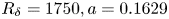 $R_\delta =1750, a=0.1629$ and
  $S=0.6732$, when large values of
  $R_\delta$ are considered, three relative maxima of
  $c_i$ appear. Indeed, for such values of the parameters, a perturbation with a dimensionless wavenumber equal to
  $0.3$ is characterized by a relative maximum of
  $c_i$ for
  $t\simeq 0.96, 2.98, 4.75$. The apparently unexpected behaviour of
  $c_i$ can be understood if the free surface time development at a fixed location is plotted vs time (see figure 7
 $b$). For
  $R_\delta =1750, a=0.1629$ and
  $S=0.6732$, the trough of the propagating wave is characterized by the presence of a small bump the height of which increases as the value of
  $R_\delta$ is increased. Therefore, for such values of the parameters, three accelerating and three decelerating phases are present during the wave cycle, whereas for smaller values of the Reynolds number only two accelerating and two decelerating phases are present. Similar results are obtained for
  $R_\delta =2000, a=0.1862, S=0.6732$ (see figure 8). Figures 7(
 $a$) and 8 show that, for large values of
  $R_\delta$, the most unstable mode is characterized by a value of the growth rate
  $c_i$ which is either positive or tends to vanish. Therefore, turbulence is expected to be present during the whole cycle and the fully developed regime to be observed, even though turbulence intensity is expected to fluctuate because of the fluctuations of
  $c_i$.

Figure 7.  $(a)$ Imaginary part
  $c_i$ of
  $c$ and
  $(b)$ free surface elevation plotted vs the phase of the wave cycle for
  $\alpha =0.3$ and
  $R_\delta =1750, a=0.1629, S=0.6732$.

Figure 8.  $(a)$ Imaginary part
  $c_i$ of
  $c$ plotted vs the phase of the wave cycle for
  $\alpha =0.3$ and
  $R_\delta =2000, a=0.1862, S=0.6732$.
It can be argued that the four flow regimes observed in a Stokes boundary layer (laminar, disturbed laminar, intermittently turbulent and fully turbulent) are present also in the boundary layer under a propagating surface wave.
A further element, which should be considered when looking at the flow under a propagating surface wave, is the roughness of the bottom. Only when the bottom is flat (no ripples) and its surface smooth (the sediment size should be much smaller than the thickness of the viscous sublayer), are the present results significant. For larger values of the sediment size, the bottom roughness certainly promotes turbulence appearance.
Of course, the linear analysis cannot describe the turbulence dynamics and only direct numerical simulations of the Navier–Stokes and continuity equations can describe the fate of the perturbations by taking into account nonlinear effects. However, it is interesting to look at the eigenfunctions in the region close to the bottom and how they decay moving far away from it. This information can give an idea of the thickening of the boundary layer when the laminar flow becomes unstable and turbulence appears. Panels  $(a)$ and
  $(b)$ of figure 9 show the eigenfunctions for
  $R_\delta =300, \alpha =0.5, S=0.6732, a=0.02793$ and two different phases of the cycle, i.e.
  $t=3{\rm \pi} /2$ and
  $t=1.8396$. The values of
  $R_\delta , \alpha$ and
  $t$ are equal to those considered in figure 3 of Blondeaux & Vittori (Reference Blondeaux and Vittori2021) and the comparison between the present results and those of figure 3 of Blondeaux & Vittori (Reference Blondeaux and Vittori2021), shows that quantitative differences are present but the qualitative behaviour of the solution is similar.

Figure 9. Real (continuous line) and imaginary (dashed line) parts of the eigenfunction  $f(z)$ for
  $R_\delta =300, \alpha =0.5, S=0.6732, a=0.02793$; (a)
  $t=1.8396$, (b)
  $t=3{\rm \pi} /2$.
The results of the analysis can be summarized by obtaining the unstable regions in the parameter space. If attention is focused on the propagating waves observed on the sea surface, the values of  $g^*$ (the gravitational acceleration) and
  $\nu ^*$ can be considered fixed and equal to
  $9.81$ ms
 $^{-2}$ and
  $10^{-6}$ m
 $^2$ s
 $^{-1}$, respectively. Then, taking into account the dispersion relationship (2.4), the value of the parameter
  $S$ follows from the knowledge of
  $h^*_0$ and
  $\omega ^*$. Moreover, if the values of
  $h^*_0$ and
  $\omega ^*$ are fixed, the parameters
  $a$ and
  $R_\delta$ are linked one to the other. Therefore, figure 10 shows the marginal stability curves in the plane
  $(\alpha ,R_\delta )$ for three different significant values of
  $S$, namely
  $0.6732, 1.622, 3.2342$ which correspond to values of the ratio
  ${h^*_0}/{L^*}$ equal to
  $0.1, 0.2$ and
  $0.3$, respectively. Smaller values of
  $S$ are not considered since, for values of
  ${h^*_0}/{L^*}$ equal to or smaller than
  $0.05$, the shallow water approach should be used to describe the wave field. On the other hand, for larger values of
  ${h^*_0}/{L^*}$, in order to have values of the Reynolds number of the bottom boundary layer close to the critical conditions, it would be necessary to consider amplitudes of the propagating surface wave which cannot be observed because they induce wave breaking.

Figure 10. Maximum value of  $c_i$ during the wave cycle plotted vs
  $\alpha$ and
  $R_\delta$ for (a)
  $S=0.6732$, i.e.
  ${h^*_0}/{L^*}=0.1$, (b)
  $S=1.622$, i.e.
  ${h^*_0}/{L^*}=0.2$, (c)
  $S=3.2342$, i.e.
  ${h^*_0}/{L^*}=0.3$. The reader should recall that, in the field, as explained in the text, the dimensionless parameter
  $a=a^*k^*$ is related to the value of the Reynolds number
  $R_\delta$.
The results shown in figure 10 show that the unstable region in the  $(\alpha , R_\delta )$-plane does not change significantly as the value of the ratio
  ${h_0^*}/{L^*}$ is changed. Therefore, only the instantaneous growth rate appears to be significantly affected the by second-order effects related to the wave steepness.
Looking at the boundaries of the unstable time intervals during the oscillation cycle plotted vs  $R_\delta$, Blondeaux & Vittori (Reference Blondeaux and Vittori2021) identified a value of the Reynolds number below which the flow regime in a Stokes boundary layer is expected to be disturbed laminar and above which intermittently turbulent. However, since only a fully nonlinear approach can describe the time development of the perturbation when the laminar regime becomes unstable, no attempt to identify a criterion to distinguish the disturbed laminar and the intermittently turbulent regime is made hereinafter. However, it can be argued that the four flow regimes (laminar, disturbed laminar, intermittently turbulent and fully turbulent) observed in a Stokes boundary layer are present also in the boundary layer under a propagating surface wave.
5. Conclusions
The linear stability analysis of the oscillating laminar flow within the boundary layer at the bottom of a propagating surface wave shows that the laminar regime is expected to be unstable and turbulence to appear when the wave amplitude is larger than a first critical value which depends on the local water depth and the period of the wave. Moreover, turbulence is predicted to appear at a given location after the passage of the wave crest when the irrotational velocity close to the bottom reverses its direction from the onshore to the offshore direction. Close to the critical conditions, the instability is predicted only during a small portion of the wave cycle. As the amplitude of the wave is increased, further unstable phases appear also after the passage of the wave trough, when the irrotational velocity close to the bottom reverses its direction from the offshore to the onshore direction. Then, the instability pervades the whole wave cycle when the amplitude of the wave becomes larger than another ‘threshold’ value. Even though this linear analysis cannot predict the time development of the perturbations when their amplitude becomes finite and it cannot be used to investigate the turbulence dynamics during the cycle, the present results along with those of Blondeaux & Vittori (Reference Blondeaux and Vittori2021) show the possible presence of different flow regimes at the bottom of a propagating surface gravity wave, i.e. the laminar regime, the disturbed laminar regime, the intermittently turbulent regime and the fully developed regime. The coherent vortex structures, which are generated by the instability of the laminar flow, and/or the small scale turbulent eddies, which are generated by the nonlinear effects, significantly affect the sediment transport rate when the sea bottom is made up of cohesionless sediments but their dynamics can be investigated only by taking into account nonlinear effects (see for example Mazzuoli et al. Reference Mazzuoli, Blondeaux, Vittori, Uhlmann, Simeonov and Calantoni2020; Vittori et al. Reference Vittori, Blondeaux, Mazzuoli, Simeonov and Calantoni2020).
Declaration of interest
The authors report no conflict of interest.
Data availability statement
The data that support the findings of this study are openly available at https://osf.io/943gu.
Author contributions
All the authors contributed equally to analysing data, reaching conclusions and in writing the paper.


 Open access