


1. Introduction
Soft materials, such as elastomers, are used to fabricate microfluidic devices (Sackmann, Fulton & Beebe Reference Sackmann, Fulton and Beebe2014). Consequently, fluid–structure interactions (FSIs) between the compliant walls and the fluids conveyed within such microconduits have emerged as a fundamental mechanics problem to understand (Christov Reference Christov2022). Previous studies have focused on the steady, inertialess flow regime. In this regime, by leveraging the FSIs, a myriad of applications to microfluidics have been proposed, such as pressure sensors (Hosokawa, Hanada & Maeda Reference Hosokawa, Hanada and Maeda2002; Ozsun, Yakhot & Ekinci Reference Ozsun, Yakhot and Ekinci2013), strain sensors (Dhong et al. Reference Dhong, Edmunds, Ramírez, Kayser, Chen, Jokerst and Lipomi2018), microrheometers with increased sensitivity (Shiba et al. Reference Shiba, Li, Virot, Yoshikawa and Weitz2021) and passive techniques for profiling microchannels’ shape (Karan et al. Reference Karan, Chakraborty, Chakraborty, Wereley and Christov2021). More recently, microfluidic systems have also begun to access inertial flow regimes up to a Reynolds number  $\textit{Re}\simeq 10^{2}$ (Di Carlo et al. Reference Di Carlo, Irimia, Tompkins and Toner2007). Although this range of $Re$ is low compared with the well-documented flow-instability $Re$ for flows in rigid conduits, flows in compliant microconduits, surprisingly, have been observed to go unstable. Dye stream experiments in a rectangular microchannel with a soft bottom wall by Verma & Kumaran (Reference Verma and Kumaran2013) showed that the stream begins to oscillate at $Re\approx 178$ and can break up at $Re\approx 200$. Other experimental studies confirmed the existence of this phenomenon, in both channels and tubes (Krindel & Silberberg Reference Krindel and Silberberg1979; Verma & Kumaran Reference Verma and Kumaran2012; Neelamegam & Shankar Reference Neelamegam and Shankar2015; Kumaran & Bandaru Reference Kumaran and Bandaru2016). Verma & Kumaran (Reference Verma and Kumaran2013) suggested that the instabilities observed are induced by FSIs. Importantly, the resulting unstable flows increased the mixing efficiency by several orders of magnitude, compared with a stable steady flow. This observation has important implications for new strategies of harnessing FSI-induced instabilities to enhance mixing at the microscale, which is notoriously challenging (Ottino & Wiggins Reference Ottino and Wiggins2004; Karnik Reference Karnik2013). Verma & Kumaran (Reference Verma and Kumaran2013) thus introduced the terms ‘ultrafast mixing’ and ‘soft-wall turbulence’ to refer these novel phenomena. However, it should be noted that FSI-induced unstable flows are fundamentally different from the usual wall-bounded turbulent flows at high $Re$ (Srinivas & Kumaran Reference Srinivas and Kumaran2015, Reference Srinivas and Kumaran2017).
Importantly, here, the low- $Re$ flows of interest are not such that $Re\to 0$. The flows of interest can be up to $Re\simeq 10^{2}$. The flow conduits in microfluidics are often manufactured to be long and slender, with a small aspect ratio $\epsilon \ll 1$ (here, defined as the ratio of radius to length for a tube, or height to length for a channel). In this context, the ‘reduced’ Reynolds number $\widehat {Re}=\epsilon Re$ is the relevant quantity to assess inertial effects in the flow because $\widehat {Re}$ is the coefficient of the inertial terms in the suitably scaled Navier–Stokes equations (as we will show in § 3). So, the observed instabilities in soft microconduits typically occur at $\widehat {Re}$ up to $O(1)$. However, for $\widehat {Re}=O(1)$, the flow can neither be considered as inertialess nor as inviscid, and we will demonstrate that there exists a balance between the fluid inertia, the dominant pressure gradient and viscous forces in the flow.
However, even at low  $Re$, analysing the instability of pressure-driven flows in compliant conduits is far more challenging than that in rigid conduits. One key challenge is that, due to FSI, the base state is not the classical unidirectional flow solution for a rigid conduit (e.g. Poiseuille or Hagen–Poiseuille flow). At steady state, a compliant channel will deform due to the hydrodynamic pressure within, and this deformation will, in turn, influence the velocity and pressure fields in the flow (Gervais et al. Reference Gervais, El-Ali, Günther and Jensen2006; Christov Reference Christov2022). Since the pressure decreases along the flow-wise direction in a pressure-driven flow, the deformation is not uniform, with larger deformation near the inlet and smaller deformation near the outlet. This non-flat shape of the deformed channel was indeed observed in the experiments by Verma & Kumaran (Reference Verma and Kumaran2013), however, its two-way coupled nature to the flow was not captured in previous stability models. Importantly, the coupling between the flow and the solid deformation gives rise to a non-constant pressure gradient in the streamwise direction, leading to a nonlinear relationship between the flow rate and the pressure drop (Gervais et al. Reference Gervais, El-Ali, Günther and Jensen2006; Seker et al. Reference Seker, Leslie, Haj-Hariri, Landers, Utz and Begley2009; Christov et al. Reference Christov, Cognet, Shidhore and Stone2018). Only a global stability analysis can take this spatially varying non-flat base state into account. However, global analyses are difficult to perform for three-dimensional (3-D) FSI problems. To this end, in the present work, we undertake reduced-order modelling.
Previous studies on instabilities due to microscale FSIs analysed the problem from the local perspective. For convenience, we term this line of research as the ‘Kumaran family’, and a list of representative studies is compared/contrasted in table 1. The Kumaran family studies typically derive a modified Orr–Sommerfeld equation by perturbing the fluid–solid interface with infinitesimal disturbances. Early studies neglected the effect of FSIs on the base state by taking the base flow to be the unidirectional one in a rigid conduit (Kumaran Reference Kumaran1995; Gaurav & Shankar Reference Gaurav and Shankar2009). Recent work by Verma & Kumaran (Reference Verma and Kumaran2013, Reference Verma and Kumaran2015) sought to improve the previous linear stability analyses by incorporating the effect of non-uniform deformation of the conduit wall. However, instead of being derived from the governing equations of two-way coupled FSI problem, the deformed shape of the channel was imaged experimentally and then reconstructed for use in computational fluid dynamics simulations. By assuming steady flow, the simulated velocity profile and the pressure distribution were taken as the base state and ‘imported’ into the linear stability analysis. Nevertheless, to arrive at an Orr–Sommerfeld equation, Verma & Kumaran (Reference Verma and Kumaran2013, Reference Verma and Kumaran2015) had to assume that the variation of the channel deformation along the streamwise direction is so slow that the flow is nearly parallel. Thus, long-wave perturbations cannot be considered, and the analysis is strictly local. Notably, the local unstable modes were predicted to arise at  $Re\lesssim 100$, both in compliant channels (Gkanis & Kumar Reference Gkanis and Kumar2005; Verma & Kumaran Reference Verma and Kumaran2013) and in compliant tubes (Verma & Kumaran Reference Verma and Kumaran2015). However, it is difficult to reach a unified understanding from the current state of this literature because the explanation regarding the onset of instability is different for each situation. For instance, considering a neo-Hookean material as the compliant wall (instead of a linearly elastic one) modifies the linear stability of the flow in a compliant tube (Gaurav & Shankar Reference Gaurav and Shankar2009). Different formulations of the linear stability analysis can also lead to completely different conclusions (Patne & Shankar Reference Patne and Shankar2019). The most recent advances and perspectives following this line of research are thoroughly reviewed by Kumaran (Reference Kumaran2021).
Table 1. Comparison of selected previous studies on instability of pressure-driven flows in complaint conduits. In the last column, ‘OS’ stands for Orr–Sommerfeld-type stability analysis; ‘RM’ stands for reduced modelling; ‘Num.’ specifically stands for two-dimensional (2-D) two-way coupled FSI simulations; ‘Asym.’ stands for asymptotic analysis; and ‘MLEE’ stands for matched local eigenfunction expansion method.
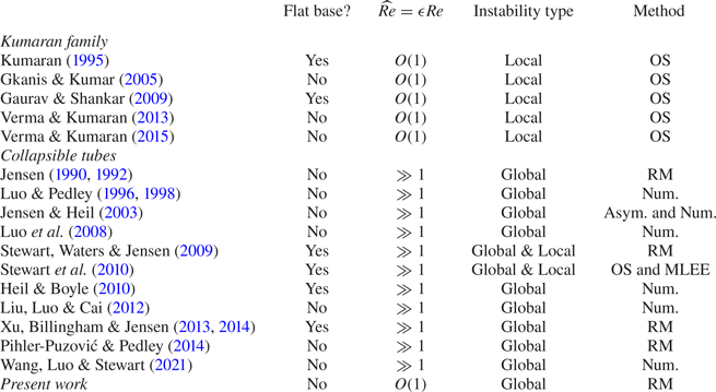
To fill these knowledge gaps, in this work, we analyse the global stability of microscale flows undergoing FSI. Specifically, we address the effect of the non-flat deformed base state, and we construct a reduced (global) model to make the analysis possible. The idea of reduced modelling is inspired by the research program on collapsible tubes; representative prior work is compared/contrasted in table 1. Although collapsible tubes research focuses on inertial flows with  $\widehat {Re}\gg 1$, and is not concerned with flows at the microscale, this research program has demonstrated the power of reduced modelling. Compared with complex two-way-coupled unsteady FSI simulations, reduced mathematical models are better suited for exploring the (potentially large) parameter space of such FSI problems. Reduced models can also aid the mathematical analysis and thus promote the understanding of the instability mechanisms. Although early one-dimensional (1-D) reduced models (Shapiro Reference Shapiro1977) incorporated ad hoc assumptions, such as an empirical tube law for deformation and an energy loss term for flow separation, these models surprisingly provided good qualitative agreement with experimental observations (Jensen & Pedley Reference Jensen and Pedley1989) and predicted the expected complex oscillations (Jensen Reference Jensen1990, Reference Jensen1992). More recently, Pihler-Puzović & Pedley (Reference Pihler-Puzović and Pedley2014) constructed a 1-D model based on the so-called interactive boundary layer theory and predicted oscillations induced by wall inertia. Meanwhile, Stewart et al. (Reference Stewart, Waters and Jensen2009) invoked the long-wave approximation and built a 1-D model to study the global and local instabilities in collapsible tubes. This model was then used extensively to investigate the effect of the pretension of the soft wall (Stewart et al. Reference Stewart, Heil, Waters and Jensen2010), the effect of the length of a downstream rigid segment (Xu et al. Reference Xu, Billingham and Jensen2013, Reference Xu, Billingham and Jensen2014) and the model was also applied to understand retinal venous pulsation (Stewart & Foss Reference Stewart and Foss2019).
Along these lines, in this work, we derive a 1-D FSI model inspired, in several ways, by the 1-D model of Stewart et al. (Reference Stewart, Waters and Jensen2009). However, instead of considering  $\widehat {Re}\gg 1$, we focus on $\widehat {Re}$ up to $O(1)$, consistent with the microchannel experiments of Verma & Kumaran (Reference Verma and Kumaran2013). The new model admits a non-flat fluid–solid interface at steady state, resulting from the nonlinear pressure distribution within the channel. We conduct a global stability analysis to properly take this spatially varying base state into account, complementary to the local stability analyses in the Kumaran family of studies. With the finite fluid inertia and non-flat base state accounted for, our 1-D FSI model is the first reduced model that addresses the global stability of pressure-driven flow in a compliant microchannel.
To this end, this paper is organized as follows. We introduce the configuration of the microchannel in § 2. In § 3, we invoke the lubrication approximation to simplify the governing equations of the internal flow. Assuming linear elasticity, we extract the dominant mechanism in the wall deformation through a scaling argument, leveraging the slenderness of the wall (§ 4.1). Then in § 4.2, the obtained displacement field is averaged over the spanwise direction ( $\hat {x}$), reducing the 3-D system (figure 1a) to a 2-D one (figure 1b). The ultimate solid model is 1-D, obtained by introducing weak inertia and modelling the weak deformation-induced tension (§ 4.3). In § 5, we couple the 1-D solid model with the depth-averaged Navier–Stokes equations to achieve a reduced 1-D FSI model relating the wall deformation to the flow rate and the pressure in the flow. We analyse the base state of the 1-D FSI model in § 6. Then in § 7, we conduct a global linear stability analysis based on the non-uniform inflated base state, the results of which are validated against unsteady numerical simulations of the 1-D FSI model (§ 8.1). The dynamics of the 1-D FSI model is also simulated by taking the undeformed state as the initial condition (§ 8.2). Finally, in § 9, we conclude with a summary of the key results of our study, and their broader context.
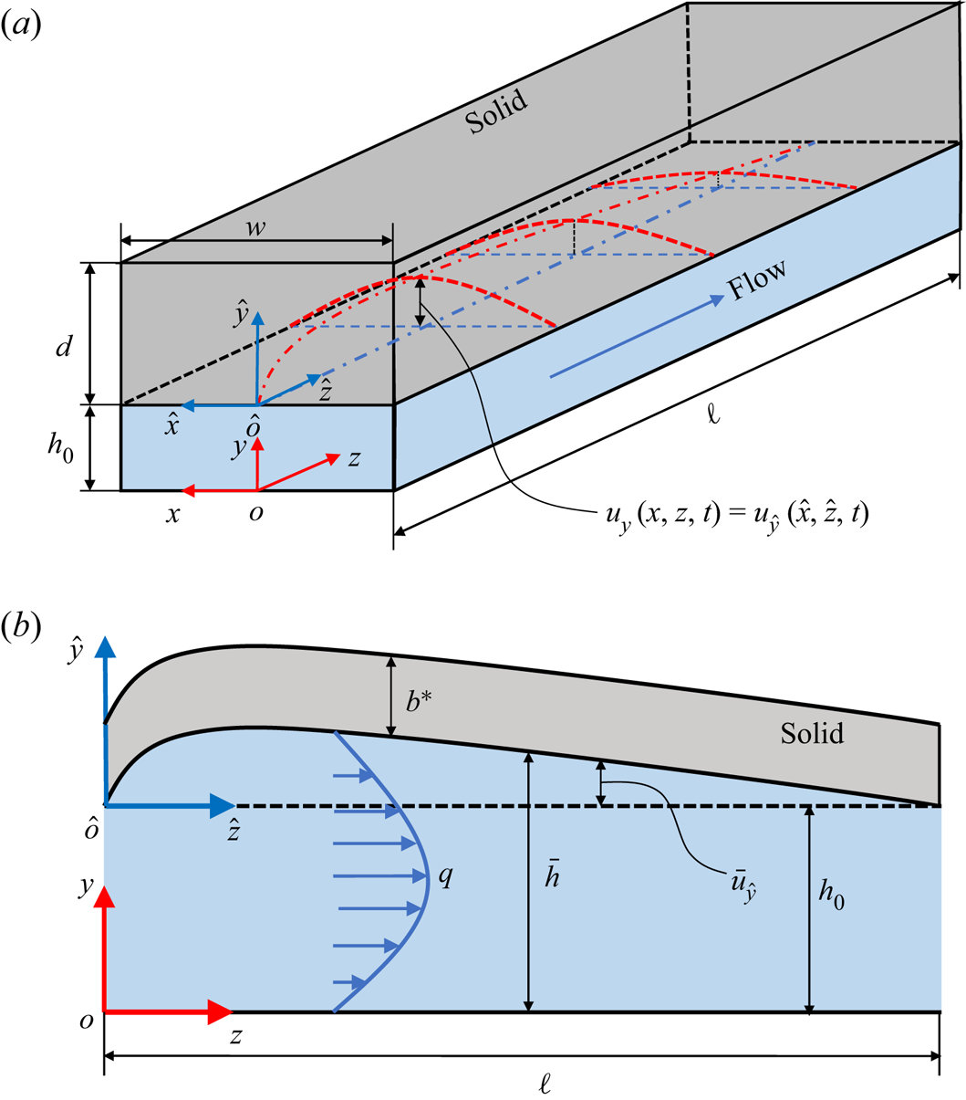
Figure 1. (a) Schematic of the 3-D geometry of the compliant microchannel with a deformable top wall (Wang & Christov Reference Wang and Christov2021), with key dimensional variables labelled. The red dash–dotted curve and the red dashed curves sketch the deformed fluid–solid interface at the midplane ( $x=0$), and the typical cross-sectional deformation profiles at the interface at different flow-wise locations, respectively. (b) Schematic of the configuration of the reduced 2-D problem obtained by width-averaging the interface displacement.
2. Problem statement
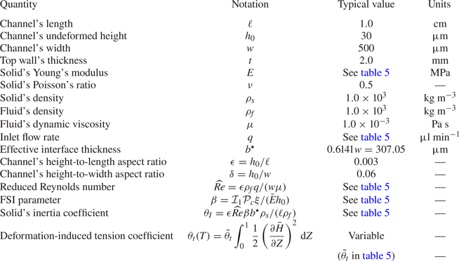
Consider a microchannel, as shown in figure 1(a), with undeformed height of  $h_0$, width of $w$ and length of $\ell$. The microchannel is assumed to be long and shallow so that $h_0\ll w\ll \ell$. Introducing the dimensionless aspect ratios $\epsilon =h_0/\ell$ and $\delta =h_0/w$, then we have $\epsilon \ll \delta \ll 1$. In reality, the three walls of the channel can be made rigid with a soft wall bonded on top, as the geometry considered in Christov et al. (Reference Christov, Cognet, Shidhore and Stone2018) and Shidhore & Christov (Reference Shidhore and Christov2018). Alternatively, the top and sidewalls are soft and bonded to a rigid bottom wall, as was the case in Wang & Christov (Reference Wang and Christov2019). In either case, the deformation of the top wall is dominant. Therefore, in our modelling, the deformation of the sidewalls is neglected. Further, we denote the thickness of the top wall by $d$. To make the model general, at this stage, we do not specify the magnitude $d$ compared with the other dimensions, but we do require that $d\ll \ell$. As the fluid is pushed through the microchannel, from the inlet to the outlet, the hydrodynamic pressure will deform the fluid–solid interface at the top wall. The displacement of the interface is denoted by $u_y(x,z,t)$. Finally, since the microchannel is often restricted from moving at the inlet ( $z=0$) and the outlet ( $z=\ell$) planes by external connections (or the outlet is open to ambient gauge pressure, thus has negligible deformation), we assume zero displacement of the fluid–solid interface at both ends ( $z=0,\ell$).
For convenience, we introduce two coordinate systems. As shown in figure 1(a), the  $o_{xyz}$ coordinate system is located at the bottom wall of the microchannel, with its origin set at the centre of the inlet. The $\hat {o}_{\hat {x} \hat {y} \hat {z}}$ coordinate system is the $o_{xyz}$ system translated along $y$ by $h_0$, thus its origin is located at the undeformed fluid–solid interface. Specifically, we have $x = \hat {x}$, $y = \hat {y}+h_0$ and $z = \hat {z}$.
3. Fluid mechanics problem formulation
3.1. Scaling and identification of the dominant effects
Assume the working fluid is incompressible and Newtonian, with a density of  $\rho _f$ and dynamic viscosity of $\mu$. With the displacement of the fluid–solid interface denoted as $u_y(x,z,t)$, the deformed channel height can be written as $h(x,z,t) = h_0 +u_y(x,z,t)$. Then, the deformed configuration of the fluid domain is $\{ (x,y,z) | -w/2\leq x \leq +w/2,\ 0\leq y\leq h(x,z,t),\ 0\leq z\leq \ell \}$. Further, we assume that $h(x,z,t)\ll w\ll \ell$, i.e. the slenderness and shallowness assumptions on the conduit hold true even after its deformation. The former assumption is important because it allows us to use $h_0$ as the scale for $y$.
$y$.
Under these assumptions, the governing equations are the unsteady incompressible Navier–Stokes equations, which take the form
 \begin{gather} \underbrace{\frac{\partial v_x}{\partial x}}_{O(1)} + \underbrace{\frac{\partial v_y}{\partial y}}_{O(1)} + \underbrace{\frac{\partial v_z}{\partial z}}_{O(1)} = 0,\end{gather}
 \begin{gather}\underbrace{\frac{\partial v_x}{\partial t}}_{O (\epsilon^{2}\delta^{{-}2}\widehat{Re})} \!+\! \underbrace{v_x\frac{\partial v_x}{\partial x}}_{O (\epsilon^{2}\delta^{{-}2}\widehat{Re})} \!+\! \underbrace{v_y\frac{\partial v_x}{\partial y}}_{O (\epsilon^{2}\delta^{{-}2}\widehat{Re})} \!+\! \underbrace{v_z\frac{\partial v_x}{\partial z}}_{O (\epsilon^{2}\delta^{{-}2}\widehat{Re})} ={-}\underbrace{\frac{1}{\rho_f}\frac{\partial p}{\partial x}}_{O(1)} \!+\! \underbrace{\frac{\mu}{\rho_f} \frac{\partial^{2} v_x}{\partial x^{2}}}_{O(\epsilon^{2})} + \underbrace{\frac{\mu}{\rho_f}\frac{\partial^{2} v_x}{\partial y^{2}}}_{O(\epsilon^{2}\delta^{{-}2})} + \underbrace{\frac{\mu}{\rho_f}\frac{\partial^{2} v_x}{\partial z^{2}}}_{O(\epsilon^{4}\delta^{{-}2})}, \end{gather}
 \begin{gather}\underbrace{\frac{\partial v_y}{\partial t}}_{O (\epsilon^{2}\widehat{Re})} + \underbrace{v_x\frac{\partial v_y}{\partial x}}_{O(\epsilon^{2}\widehat{Re})} + \underbrace{v_y\frac{\partial v_y}{\partial y}}_{O (\epsilon^{2}\widehat{Re})} + \underbrace{v_z\frac{\partial v_y}{\partial z}}_{O(\epsilon^{2}\widehat{Re})} ={-}\underbrace{\frac{1}{\rho_f}\frac{\partial p}{\partial y}}_{O(1)} + \underbrace{\frac{\mu}{\rho_f} \frac{\partial^{2} v_y}{\partial x^{2}}}_{O(\epsilon^{2} \delta^{2})} + \underbrace{\frac{\mu}{\rho_f}\frac{\partial^{2} v_y}{\partial y^{2}}}_{O(\epsilon^{2})} + \underbrace{\frac{\mu}{\rho_f}\frac{\partial^{2} v_y}{\partial z^{2}}}_{O(\epsilon^{4})}, \end{gather}
 \begin{gather}\underbrace{\frac{\partial v_z}{\partial t}}_{O (\widehat{Re})} + \underbrace{v_x\frac{\partial v_z}{\partial x}}_{O(\widehat{Re})} + \underbrace{v_y \frac{\partial v_z}{\partial y}}_{O(\widehat{Re})} + \underbrace{v_z\frac{\partial v_z}{\partial z}}_{O (\widehat{Re})} ={-}\underbrace{\frac{1}{\rho_f} \frac{\partial p}{\partial z}}_{O(1)} + \underbrace{\frac{\mu}{\rho_f}\frac{\partial^{2} v_z}{\partial x^{2}}}_{O(\delta^{2})} + \underbrace{\frac{\mu}{\rho_f} \frac{\partial^{2} v_z}{\partial y^{2}}}_{O(1)} + \underbrace{\frac{\mu}{\rho_f}\frac{\partial^{2} v_z}{\partial z^{2}}}_{O(\epsilon^{2})}, \end{gather}
with the order of magnitude of each term listed underneath, based on the scales from table 2.
Table 2. The scales for the variables in the incompressible Navier–Stokes equations (3.1).
In table 2,  $\mathcal {V}_c$ is the characteristic velocity scale. Specifically, to ensure the conservation of mass of (3.1a), $\epsilon \mathcal {V}_c/\delta$, $\epsilon \mathcal {V}_c$ and $\mathcal {V}_c$ are chosen to be the characteristic scales for the velocity components $v_x$, $v_y$ and $v_z$, respectively. Also, as is standard for low-Reynolds-number flow, to achieve a balance between the pressure and the viscous stresses in (3.1d), the characteristic pressure scale, $\mathcal {P}_c$, and $\mathcal {V}_c$ are related by $\mathcal {P}_c=\mu \mathcal {V}_c \ell /h_0^{2}$. If the volumetric flow rate, $q$, at the inlet is fixed, we can choose $\mathcal {V}_c = q/(wh_0)$, then $\mathcal {P}_c = \mu q \ell /(wh_0^{3})$. However, if the pressure drop, ${\rm \Delta} p = p|_{z=0}- p|_{z=\ell }$, is prescribed, $\mathcal {P}_c = {\rm \Delta} p$ and, accordingly, $\mathcal {V}_c = {\rm \Delta} p h_0^{2}/(\mu \ell )$. The Reynolds number is defined as $Re=\rho _f\mathcal {V}_c h_0/{\mu }$. However, owing to the shallowness and slenderness of the fluid domain ( $\epsilon \ll \delta \ll 1$), the inertial effects in the $z$-momentum equation (3.1d) are more dominant than in the other two momentum equations. In this scaling, $\widehat {Re}=\epsilon Re$ emerges as the sole prefactor of the inertial terms in (3.1d) (rather than $Re$), thus we say that the reduced Reynolds number $\widehat {Re}$ is more suitable for quantifying the inertia of this flow. Finally, $\mathcal {T}_f$ is taken to be the characteristic time scale for axial advection (the dominant flow direction): $\mathcal {T}_f=\ell /\mathcal {V}_c$.
3.2. Reduction: lubrication approximation
Recall that we are interested in flow in a shallow and slender microchannel ( $h_0\ll w\ll \ell$) such that $\epsilon =h_0/\ell \ll \delta =h_0/w \ll 1$. Based on the discussion above, it is clear that the dominant balance of terms occurs in the $z$-momentum equation (3.1d). Only the pressure terms are left in (3.1b) and (3.1c), indicating that, at the leading order in $\epsilon$ and $\delta$, the hydrodynamic pressure $p$ is only a function of the streamwise location $z$, as in the classic lubrication approximation (White Reference White2006; Panton Reference Panton2013). More importantly, this argument is true even at finite Reynolds number, i.e. $\widehat {Re}= O(1)$, which is typical of the microfluidic experiments of Verma & Kumaran (Reference Verma and Kumaran2013) that we compare with. Specifically, with $\widehat {Re}= O(1)$, the dominant balance in the flow-wise momentum equation (3.1d) occurs between fluid inertia, the pressure gradient and viscous forces. The same balance was employed by Inamdar, Wang & Christov (Reference Inamdar, Wang and Christov2020) to derive a 1-D FSI model from the 2-D Navies–Stokes equations (but under different assumptions on the solid mechanics problem).
Examining further the right-hand side of (3.1d), the balance of forces at the leading order indicates that  $\partial p/\partial z \sim \partial \tau _{yz}/\partial y$ because the shear stress is $\tau _{yz} \sim \mu \partial v_z/\partial y$. Introducing $\mathcal {S}_c$ as the characteristic scale for $\tau _{yz}$ and substituting the other scales from table 2, this balance suggests that $\mathcal {P}_c/\ell = \mathcal {S}_c/h_0$, leading to $\mathcal {S}_c=(h_0/\ell) \mathcal {P}_c=\epsilon \mathcal {P}_c$. For $\epsilon \ll 1$, we conclude that $\tau _{yz}\ll p$. Hence, at the leading order in $\epsilon$ and $\delta$, $p(z)$ is the only flow-induced load exerted on the fluid–solid interface.
4. Solid mechanics problem formulation
4.1. Scaling and identification of the dominant effects
For the solid mechanics problem, it is more convenient to use the  $\hat {o}_{\hat {x} \hat {y} \hat {z}}$ coordinate system, where we denote the displacement of the fluid–solid interface by $u_{\hat {y}}$, as shown in figure 1(a). We consider the case in which the maximum of $\hat {u}_y$ is small compared with the smallest dimension of the solid, so that the small-strain theory of linear elasticity is applicable. Specifically, if the wall is ‘thick’, meaning $w \lesssim d \ll \ell$, we require that $\hat {u}_y \ll w$. However, if the wall is ‘thin’, meaning $d\lesssim w \ll \ell$, we require that $\hat {u}_y \ll d$ (Wang & Christov Reference Wang and Christov2021).
The following discussion proceeds along the lines of Wang & Christov (Reference Wang and Christov2019). However, here, we provide a more general derivation for the reader's convenience. First, using the scales from table 3, the balance between the Cauchy stresses and the solid inertia within the wall, neglecting any body forces, is
 \begin{gather} \underbrace{\rho_s\frac{\partial^{2} u_{\hat{x}}}{\partial t^{2}}}_{O(\rho_s \mathcal{U}_{c,x}/\mathcal{T}_f^{2}) } + \underbrace{\frac{\partial \sigma_{\hat{x} \hat{x}}}{\partial \hat{x}}}_{O({\mathcal{D}_{\hat{x} \hat{x}}}/{w})} + \underbrace{\frac{\partial \sigma_{\hat{x} \hat{y}}}{\partial \hat{y}}}_{O({\mathcal{D}_{\hat{x} \hat{y}}}/{d})} + \underbrace{\frac{\partial \sigma_{\hat{x} \hat{z}}}{\partial \hat{z}}}_{O({\mathcal{D}_{\hat{x} \hat{z}}}/{\ell})} = 0, \end{gather}
 \begin{gather}\underbrace{\rho_s\frac{\partial^{2} u_{\hat{y}}}{\partial t^{2}}}_{O(\rho_s\mathcal{U}_c/\mathcal{T}_f^{2})} + \underbrace{\frac{\partial \sigma_{\hat{x} \hat{y}}}{\partial \hat{x}}}_{O({\mathcal{D}_{\hat{x} \hat{y}}}/{w})} + \underbrace{\frac{\partial \sigma_{\hat{y} \hat{y}}}{\partial \hat{y}}}_{O(\mathcal{P}_c/{d})} + \underbrace{\frac{\partial \sigma_{\hat{y} \hat{z}}}{\partial \hat{z}}}_{O(\epsilon\mathcal{P}_c/\ell)} = 0, \end{gather}
 \begin{gather}\underbrace{\rho_s\frac{\partial^{2} u_{\hat{z}}}{\partial t^{2}}}_{O(\rho_s \mathcal{U}_{c,z}/\mathcal{T}_f^{2})} + \underbrace{\frac{\partial \sigma_{\hat{x} \hat{z}}}{\partial \hat{x}}}_{O({\mathcal{D}_{\hat{x} \hat{z}}}/{w})} + \underbrace{\frac{\partial \sigma_{\hat{y} \hat{z}}}{\partial \hat{y}}}_{O(\epsilon\mathcal{P}_c/{d})} + \underbrace{\frac{\partial \sigma_{\hat{z} \hat{z}}}{\partial \hat{z}}}_{O({\mathcal{D}_{\hat{z} \hat{z}}}/{\ell})} = 0. \end{gather}
Here,  $\sigma _{\hat {x} \hat {x}}$, $\sigma _{\hat {x} \hat {y}}$, $\sigma _{\hat {x} \hat {z}}$, $\sigma _{\hat {y} \hat {y}}$, $\sigma _{\hat {y} \hat {z}}$ and $\sigma _{\hat {z} \hat {z}}$ are the six independent components of the Cauchy stress in the solid. The order of magnitude of each term is listed underneath, based on the scales from table 3.
Table 3. The scales for the variables in the linear elastodynamics equations (4.1).
In table 3,  $\mathcal {U}_{c,x}$, $\mathcal {U}_c$ and $\mathcal {U}_{c,z}$ are the characteristic scales for $u_{\hat {x}}$, $u_{\hat {y}}$ and $u_{\hat {z}}$, respectively. We immediately assume that $\mathcal {U}_{c,x}\ll \mathcal {U}_c$ and $\mathcal {U}_{c,z}\ll \mathcal {U}_c$, meaning that the wall is primarily bulging upwards, as in experiments. This assumption has previously been quantitatively validated against experiments (Christov et al. Reference Christov, Cognet, Shidhore and Stone2018; Shidhore & Christov Reference Shidhore and Christov2018; Wang & Christov Reference Wang and Christov2019). Then the most prominent inertial term in the solid is in (4.1b). Note that the time scale for (4.1) is still the fluid's axial advection time scale, $\mathcal {T}_f$, in order to ensure the coupling between the solid and the fluid mechanics problems. Note that this choice of time scale is different from the so-called ‘viscous–elastic’ one used in related works (Elbaz & Gat Reference Elbaz and Gat2014; Martínez-Calvo et al. Reference Martínez-Calvo, Sevilla, Peng and Stone2020). In the latter papers, the characteristic (common) time scale $\mathcal {T}_c$ was chosen based on the kinematic boundary condition at the fluid–solid interface, i.e. $\partial \bar {u}_y/\partial t = v_y$, leading to a fluid time scale of $\mathcal {T}_c=\bar {\mathcal {U}}_c/(\epsilon \mathcal {V}_c) = (\bar {\mathcal {U}}_c/h_0)(\ell /\mathcal {V}_c)= \beta \mathcal {T}_f$. However, since $\beta=\bar{\mathcal{U}}_c/h_0$ is typically at $O(1)$ in our work (discussed in § 4.4), these two different choices of the fluid time scale, $\mathcal {T}_c$ and $\mathcal {T}_f$, do not differ significantly. To further elucidate the time scales involved, the magnitude of the inertial term in (4.1b) can be written as $\rho _s\mathcal {U}_c/\mathcal {T}_f^{2}=\rho _s\mathcal {U}_c/\mathcal {T}_s^{2} \times (\mathcal {T}_s/\mathcal {T}_f)^{2}$, where we have explicitly introduced the solid time scale, $\mathcal {T}_s$. Note that when the soft solid's density is similar to the fluid's density (see example values in table 4 below), the elastic wave speed in the solid is $\sqrt {E/\rho _s}\gg \mathcal {V}_c$. Therefore, the development of the solid deformation is expected to be much faster than the flow, i.e. $\mathcal {T}_s \ll \mathcal {T}_f$, which makes the solid's inertia a weak effect. We will quantify the solid's weak inertia in § 4.4, but for now it can be neglected to find the deformation profile (bulging of the fluid–solid interface due to the hydrodynamic pressure).
Table 4. The dimensional and dimensionless parameters of the 1-D FSI model.
To this end, let us consider the balance of the Cauchy stresses in (4.1). Due to the traction balance at the fluid–solid interface, it can be inferred that  $\mathcal {D}_{\hat {y}\hat {y}} = \mathcal {P}_c$ and $\mathcal {D}_{\hat {y} \hat {z}} = \epsilon \mathcal {P}_c$, as tabulated in table 3. For convenience, we introduce $\gamma = d/w$ as the spanwise aspect ratio of the solid wall. Then, a balance in (4.1b) can only occur between the second and the third terms, yielding $D_{\hat {x} \hat {y}} = \mathcal {P}_c/\gamma$. At the same time, the balance of the three terms in (4.1c) gives $\mathcal {D}_{\hat {x} \hat {z}} = \epsilon \mathcal {P}_c w/d = \epsilon \mathcal {P}_c/\gamma$ and $\mathcal {D}_{\hat {z} \hat {z}} = \epsilon \mathcal {P}_c\ell /d = \delta \mathcal {P}_c/\gamma$. Finally, from (4.1a), the only remaining possibility is that the second term balances the third term, indicating $\mathcal {D}_{\hat {x} \hat {x}}=w\mathcal {D}_{\hat {x} \hat {y}}/d = \mathcal {P}_c/\gamma ^{2}$.
So far, we have only required that the elastic solid is slender, i.e.  $d\ll \ell$, which is equivalent to $\gamma \ll \delta /\epsilon$, and covers a large range of wall thicknesses (recall that $\gamma =d/w$, $\epsilon =h_0/\ell$ and $\delta =h_0/w$). However, it is also expected that $\gamma \gg \epsilon$, such that $\mathcal {D}_{\hat {x} \hat {z}}$ is a small quantity, excluding the case of an extremely thin wall. In fact, recalling that the application of linear elasticity requires that $\hat {u}_y\ll d$, any prominent deformation in a thin-walled microchannel is likely beyond the scope of the linear elastic theory.
Therefore, with  $\epsilon \ll \gamma \ll \delta /\epsilon$ as well as $\epsilon \ll \delta \ll 1$, we conclude that $\sigma _{\hat {x} \hat {z}}$ and $\sigma _{\hat {y} \hat {z}}$ are negligible in comparison with the other stress components. Depending on the wall thickness, the relative magnitude among the remaining four stress components can change. For example, if $\gamma ^{2} \gg 1$, we can further neglect $\sigma _{\hat {x} \hat {x}}$ as in Wang & Christov (Reference Wang and Christov2019). Nevertheless, no matter how $d$ varies, the dominant balances in (4.1a) and (4.1b) occur in the cross-sectional $(\hat {x},\hat {y})$ plane, which reduces the original 3-D elasticity problem to a 2-D plane-strain problem. Since we showed in § 3 that $p$ is a function of $z$ only at the leading order (in $\epsilon$), the deformation of the $(\hat {x},\hat {y})$ cross-sections at different $z$-locations (recalling $z=\hat {z}$) decouple from each other. At each cross-section, the deformation is then determined by the local hydrodynamic pressure $p(z,t)$. Therefore, generally, we can express the displacement of the fluid–solid interface at the leading order (in $\epsilon$) as
 \begin{equation} u_y(x,z,t) = u_{\hat{y}}(\hat{x}, \hat{z}, t)= \mathfrak{f}(x)p(z,t), \end{equation}
with  $\mathfrak {f}(x)$ being the spanwise deformation profile. The separation-of-variables form of (4.2) suggests that the cross-sectional deformation profiles at different $z$-locations are, in a sense, self-similar. The displacement is fully determined by the local pressure, showing that the fluid–solid interface behaves like a Winkler foundation (Winkler Reference Winkler1867; Dillard et al. Reference Dillard, Mukherjee, Karnal, Batra and Frechette2018), with a variable stiffness represented by $1/\mathfrak {f}(x)$. Importantly, this Winkler-foundation-like mechanism is not an assumption here, but rather it is a consequence of the slenderness of the top wall. Also, note that the assumption of $\mathcal {T}_s\ll \mathcal {T}_f$ has been applied here, meaning that the solid promptly responds to pressure changes in the flow.
It is also worth mentioning that if the top wall is thin with  $\epsilon \ll \gamma \lesssim 1$, the elasticity problem is usually taken to be a plane stress problem, and a 1-D engineering model is usually available for the displacement out of plane (i.e. $u_y$ here), such as the Kirchhoff–Love (Love Reference Love1888; Timoshenko & Woinowsky-Krieger Reference Timoshenko and Woinowsky-Krieger1959) and Reissner–Mindlin (Reissner Reference Reissner1945; Mindlin Reference Mindlin1951) plate theories. However, this fact does not fundamentally contradict with our plane-strain reduction because the decoupling of the cross-sections remains true (Christov et al. Reference Christov, Cognet, Shidhore and Stone2018; Shidhore & Christov Reference Shidhore and Christov2018; Anand, Muchandimath & Christov Reference Anand, Muchandimath and Christov2020) due to the separation of scales, $w\ll \ell$.
Moreover, the discussion above is only based on the balance of Cauchy stresses, and does not involve the boundary conditions either on the sides (i.e. at  $x=\pm w/2$) or at the upper surface of the wall (i.e. at $\hat {y}=d$ or $y=h_0 +d$). The decoupling of the cross-sectional deformation is just a consequence of the wall slenderness. However, the boundary conditions do have an important influence on the displacement field in the solid, which gives rise to different forms of $\mathfrak {f}(x)$ in (4.2) (Wang & Christov Reference Wang and Christov2021).
4.2. Reduction: introducing the width-averaged (effective) height
Since we seek a 1-D model dependent on  $z$ only, the $x$-dependence can be eliminated by averaging the displacement of the fluid–solid interface over $x$:
$x$:
 \begin{equation} \bar{u}_y(z,t) = \frac{1}{w}\int_{{-}w/2}^{{+}w/2} u_y(x,z,t)\, \mathrm{d}\kern0.06em x = \underbrace{\left[ \frac{1}{w}\int_{{-}w/2}^{{+}w/2} \mathfrak{f}(x)\, \mathrm{d}\kern0.06em x\right]}_{1/k} p(z,t), \end{equation}
having used (4.2). Then, the width-averaged height  $\bar {h}$ of the channel is
 \begin{equation} \bar{h}(z,t) = \frac{1}{w}\int_{{-}w/2}^{{+}w/2} h_0 + u_y(x,z,t)\, \mathrm{d}\kern0.06em x = h_0 + \frac{1}{k}p(z,t). \end{equation}
An important quantity in the above equations is the proportionality constant,  $k$, which represents the effective stiffness of the interface and further highlights the Winkler-foundation-like mechanism of deformation of the fluid–solid interface.
Equation (4.4) simplifies the FSI problem in two aspects. First, the deformation of the interface is further reduced from 2-D to 1-D. Second, the flow in the channel is reduced from 3-D to 2-D, and this reduction does not change any key statements made before because we can still appeal to the lubrication approximation for 2-D flows due to  $h_0\ll \ell$. In other words, if we start from the 2-D incompressible Navier–Stokes equations (simply neglecting $v_x$ and $x$-dependent terms), we still find the lubrication approximation is applicable up to $\widehat {Re} = O(1)$, as in § 3.2.
In the following discussion, we will take  $\bar {h}$ as the effective height of the deformed channel and consider the reduced system sketched in figure 1(b). Note that the 2-D configuration in figure 1(b) is not a priori assumed but, rather, it is derived from the 3-D configuration in figure 1(a) based on averaging the deformation across $x$, via (4.3) (or (4.4)). This approach is in contrast to the earlier work of, e.g. Skotheim & Mahadevan (Reference Skotheim and Mahadevan2004), who assumed a 2-D configuration of the elastic solid in the $(y,z)$ plane from the outset. Taking $\bar {h}$ as the effective deformed height was first suggested by Gervais et al. (Reference Gervais, El-Ali, Günther and Jensen2006). As shown by Wang & Christov (Reference Wang and Christov2021), the error introduced by this averaging approach is controllable.
4.3. Extension: introducing weak deformation effects
So far, the discussion in the previous subsections was based on the leading-order (in  $\epsilon$) theory, which does not take into account the possible restrictions imposed at the inlet and the outlet (i.e. at $z=0$ and $z=\ell$). As shown in figure 1(b), the movement of the fluid–solid interface at both ends is often physically restricted. In this sense, we can think of the solid mechanics problem as being essentially a boundary layer problem. While the Winkler-foundation-like mechanism is dominant outside any ‘boundary layers’, with (4.3) being the (outer) solution there, another mechanism plays a role within thin (boundary) layers near $z=0,\ell$, each potentially admitting inner solutions that regularize the problem and allow the enforcement of end constraints.
Since the bulging of the top wall unavoidably introduces stretching along  $z$ in the solid, a simple extension of (4.3) can be achieved by introducing weak constant tension into the formulation (Wang & Christov Reference Wang and Christov2021). First, for the Winkler-foundation-like mechanism to be dominant, the tension needs to be ‘weak’. Second, the tension force can be taken to be constant because its variation along $z$ is proportional to the fluid's tangential traction at the interface, which is a small quantity per the lubrication approximation, as shown in § 3 (see also Hewitt, Balmforth & De Bruyn Reference Hewitt, Balmforth and De Bruyn2015). The ‘regularized’ governing equation for the width-averaged fluid–solid interface's displacement $\bar {u}_y$ is then written as
 \begin{equation} \underbrace{\rho_s
b^{{\star}} \frac{\partial^{2} \bar{u}_y}{\partial
t^{2}}}_{\text{inertia}} + \underbrace{k\bar{u}_y}_{\text{stiffness}}
- \underbrace{\chi_t\frac{\partial^{2} \bar{u}_y}{\partial
z^{2}}}_{\text{tension}} = \underbrace{p(z,t)}_{\text{load}},
\end{equation}
\begin{equation} \underbrace{\rho_s
b^{{\star}} \frac{\partial^{2} \bar{u}_y}{\partial
t^{2}}}_{\text{inertia}} + \underbrace{k\bar{u}_y}_{\text{stiffness}}
- \underbrace{\chi_t\frac{\partial^{2} \bar{u}_y}{\partial
z^{2}}}_{\text{tension}} = \underbrace{p(z,t)}_{\text{load}},
\end{equation}
where  $\rho _s$ denotes the solid density, $b^{\star }$ represents the effective thickness of the interface (discussed in § A.1), which is introduced so that the first term can represent the bulk inertial effects of the solid. Recalling that $k$ is the effective stiffness introduced from (4.3), the second term represents the dominant Winkler-foundation-like effect, while $\chi _t$ is introduced to model the tension per unit width (discussed in § A.2). In the case of $\chi _t$ being constant, the tension can be written in terms of the transverse displacement $\bar {u}_y$ (see e.g. Howell, Kozyreff & Ockendon (Reference Howell, Kozyreff and Ockendon2009), § 4.3). The weakness of the solid inertia and the tension may not be obvious from (4.5), although the scaling analysis in § 4.1 anticipates it.
Equation (4.5) is essentially the equation of motion of a Kramer-type surface, which has been used extensively in the study of high- $Re$ (boundary layer) flows over compliant coatings. The goal of the latter studies is to understand how to delay the laminar–turbulence transition (Gad-el Hak Reference Gad-el Hak2002). However, microchannel flows cannot reach such high $Re$ values. More surprisingly, the application of (4.5) in modelling soft microchannels leads to different conclusions from the compliant coating studies. Compliance of the channel wall can actually promote (instead of delay) the laminar–turbulence transition in pressure-driven flow thanks to the FSI-induced instabilities. This effect can be successfully exploited for micromixing.
4.4. Non-dimensionalization: introducing the FSI parameter
We can now make the 1-D interface motion equation (4.5) dimensionless to better illustrate the relative magnitude of the different terms (effects). Capital letters are used to denote the dimensionless variables.
The first step is to determine the characteristic scale,  $\bar {\mathcal {U}}_c$, for the fluid–solid interface displacement. The dominant deformation effect in (4.3), suggests that we should take $\bar {\mathcal {U}}_c = \mathcal {P}_c/k$, recalling that the scale for $p$ is $\mathcal {P}_c$. Then, the dimensionless version of (4.3) is simply
 \begin{equation} \bar{U}_Y(Z,T) = P(Z,T). \end{equation}
Still using  $h_0$ to scale $\bar {h}$, the dimensionless effective channel height (see (4.4)) becomes
 \begin{equation} \bar{H}(Z,T) = 1 + \frac{\bar{\mathcal{U}}_c}{h_0}\bar{U}_Y(Z,T) = 1 + \beta \bar{U}_Y(Z,T). \end{equation}
Here, we have introduced another dimensionless parameter,  $\beta =\bar {\mathcal {U}}_c/h_0=\mathcal {P}_c/(kh_0)$. It is clear from (4.7) that $\beta$ translates the interface displacement into the deformation of the fluid domain, capturing the ‘strength’ of the fluid–solid coupling. Thus, $\beta$ is the ‘FSI parameter’ of our model.
The dependence of  $\beta$ on the system properties comes through $\mathcal {P}_c$ and $k$. While $\mathcal {P}_c$ is determined by the flow conditions (i.e. the viscosity of the fluid, the flow rate and the geometry of the undeformed channel), $k$ is determined by the material properties, the geometry and the boundary conditions on the compliant wall. To explicitly show this, we write
 \begin{equation} \frac{1}{k} = \frac{1}{w}\int_{{-}w/2}^{{+}w/2} \mathfrak{f}(x)\, \mathrm{d}\kern0.06em x= \int_{{-}1/2}^{{+}1/2} \mathfrak{f}(wX)\, \mathrm{d}\kern0.06em X = \frac{\xi}{\bar{E}}\underbrace{\int_{{-}1/2}^{{+}1/2} F(X)\, \mathrm{d}\kern0.06em X}_{\mathcal{I}_1}= \frac{\xi\mathcal{I}_1}{\bar{E}}. \end{equation}
The definition of  $k$ from (4.3) is used in the first step. The second step is making the integral dimensionless. In the third step, the assumption of a linearly elastic solid has been invoked with $k\propto \bar {E}$ and $\mathfrak {f}(x)\propto 1/\bar {E}$. Note that $\bar {E} = E/(1-\nu _s^{2})$ here, which means that $k$ is well defined as $\nu _s\to 1/2^{-}$, because of the plane-strain reduction from 3-D to 2-D, with $E$ being Young's modulus and $\nu _s$ being the Poisson ratio, respectively. Then, $F(X)$ is introduced as the dimensionless self-similar deformation profile, and $\xi$ is the resulting prefactor after $x$ is scaled by $w$. In the last step, $\mathcal {I}_1=\int _{-1/2}^{+1/2} F(X)\, \mathrm {d}\kern0.06em X$ was introduced to simplify the expression. While the effect of the material properties of the solid wall are captured by $\bar {E}$, the influence of the wall geometry and the boundary conditions are taken into account by both $\xi$ and $\mathcal {I}_1$. As mentioned in § 4.1, $\mathfrak {f}(x)$ takes different forms in different situations, thus giving different expressions for $\xi$ and $\mathcal {I}_1$. For example, for the thick-walled microchannel considered by Wang & Christov (Reference Wang and Christov2019), $\xi =w$ and $\mathcal {I}_1\approx 0.542754$. Meanwhile, for the microchannels with thick-plate-like top walls considered by Shidhore & Christov (Reference Shidhore and Christov2018), $\xi =w^{4}/(2d^{3})$ and $\mathcal {I}_1={1}/{30}+{(d/w)^{2}}/[{3\kappa (1-\nu _s)}]$, with $\kappa$ being a ‘shear correction factor’ (typically, $\kappa =1$). Nevertheless, the key point is that both $\xi$ and $\mathcal {I}_1$ can be obtained a priori, by solving the corresponding elasticity problem, as analytical expressions.
Using the scales from tables 2 and 3, the dimensionless version of (4.5) is
 \begin{equation} \theta_I \frac{\partial^{2} \bar{U}_Y}{\partial T^{2}} + \bar{U}_Y -\theta_t\frac{\partial^{2} \bar{U}_Y}{\partial Z^{2}} = P, \end{equation}
where  $\theta _I = \rho _s b^{\star }\mathcal {\bar {U}}_c/(\mathcal {T}_f^{2} \mathcal {P}_c)$ and $\theta _t = \chi _t \bar {\mathcal {U}}_c/(\ell ^{2}\mathcal {P}_c)$ are introduced above as the inertial coefficient and the tension coefficient, respectively. We expect that $\theta _I\ll 1$ and $\theta _t\ll 1$ because both the solid inertia and the tension effect are weak. Then, the leading-order solution (as $\theta _I,\theta _t\to 0$) of (4.9) is (4.6), as required by the above discussion. Even though $\theta _I\ll 1$ and $\theta _t\ll 1$, it is important to properly model these weak effects because they have significant influence on the global instability of the system (as we will see in § 7.1).
First, let us justify  $\theta _I\ll 1$. Recalling that $\mathcal {P}_c=\mu \mathcal {V}_c/(\epsilon h_0)$, $\widehat {Re}=\epsilon \rho _f\mathcal {V}_c h_0/\mu$, and $\beta = \bar {\mathcal {U}}_c/h_0$, $\theta _I$ can be written as
 \begin{equation} \theta_I = \frac{\rho_s b^{{\star}}\mathcal{\bar{U}}_c}{\mathcal{T}_f^{2} \mathcal{P}_c}= \epsilon\frac{\rho_f\mathcal{V}_ch_0}{\mu}\frac{\mathcal{\bar{U}}_c}{{h_0}}\frac{b^{{\star}}h_0}{\ell^{2}}\frac{\rho_s}{\rho_f} = \epsilon \widehat{Re}\beta\frac{b^{{\star}} }{\ell }\frac{\rho_s}{\rho_f}. \end{equation}
Since  $\epsilon \ll 1$, $b^{\star } \leq d\ll \ell$, $\widehat {Re}= O(1)$, $\beta$ is typically $O(1)$ and $\rho _s\simeq \rho _f$ in the microchannel setting (because polydimethylsiloxane (known as PDMS) has a similar density to water), we have justified $\theta _I\ll 1$. Note that time in (4.5) is scaled by $\mathcal {T}_f$, as before, to ensure the fluid–solid coupling. Thus, $\theta _I\ll 1$ corresponds to $\mathcal {T}_s^{2}\ll \mathcal {T}_f^{2}$, meaning that the solid responds to pressure changes in the flow promptly, as discussed in § 4.1. It is also helpful to note that, using (4.8), we can also write
 \begin{equation} \theta_I = \mathcal{I}_1\frac{\rho_s b^{{\star}} \xi}{\mathcal{T}_f^{2} \bar{E}}, \end{equation}
which indicates that, for a more rigid solid (i.e. with the increase of  $\bar {E}$), the solid deformation develops much faster than the flow.
Next, using (4.8) again, the dimensionless tension coefficient can be written as
 \begin{equation} \theta_t = \frac{\chi_t \bar{\mathcal{U}}_c}{\ell^{2}\mathcal{P}_c} =\mathcal{I}_1\frac{\chi_t \xi}{\bar{E}\ell^{2}}. \end{equation}
If  $\chi _t$ is deformation-induced (thus time-dependent), substituting equation (A3) into (4.12), we obtain
 \begin{align} \theta_t(T) &=\mathcal{I}_1\frac{\xi}{\bar{E}\ell^{2}} \frac{E b^{{\star}}}{\ell} \int_0^{\ell} \frac{1}{2}\left(\frac{\partial \bar{u}_y}{\partial z}\right)^{2}\, \mathrm{d} z \nonumber\\ &= (1-\nu_s^{2})\mathcal{I}_1 \frac{\xi b^{{\star}}\bar{\mathcal{U}}_c^{2} }{\ell^{4}} \int_0^{1} \frac{1}{2} \left(\frac{\partial \bar{U}_Y}{\partial Z}\right)^{2} \, \mathrm{d} Z \nonumber\\ &= \tilde{\theta}_t \int_0^{1} \frac{1}{2} \left(\frac{\partial \bar{H}}{\partial Z}\right)^{2} \, \mathrm{d} Z, \end{align}
where
 \begin{equation} \tilde{\theta}_t = \frac{1}{\beta^{2}}\times (1-\nu_s^{2})\mathcal{I}_1 \frac{\xi b^{{\star}}\bar{\mathcal{U}}_c^{2} }{\ell^{4}} =(1-\nu_s^{2})\mathcal{I}_1 \epsilon^{2}\frac{\xi b^{{\star}}}{\ell^{2}}. \end{equation}
Note that we have used (4.7) in the last step of the manipulations in (4.13). Also, note that  $\tilde {\theta }_t$ is not related to the flow conditions, and $\tilde {\theta }_t \ll 1$ for microchannels. Within linear elasticity, the integral in (4.13) is $O(1)$, thus $\theta _t\ll 1$ as well.
Finally, the key dimensional and dimensionless parameters are summarized in table 4. Typical values for microfluidic systems are given to justify the bigness/smallness assumptions made.
5. Fluid–solid coupling: a new 1-D FSI model
The final step in deriving the 1-D FSI model involves coupling the fluid mechanics problem to the solid mechanics problem. This coupling is achieved by depth averaging the Navier–Stokes equations at the leading order in  $\epsilon$. Recall that, even though we averaged across $X$ in § 4.2, the flow field is 2-D at this stage, i.e. $V_Z=V_Z^{2D}(Y,Z,T)$. Vertically integrating the axial velocity, $V_Z^{2D}$, introduces the flow rate, $Q(Z,T) = \int _{0}^{\bar {H}(Z,T)}V_Z^{2D}(Y,Z,T)\,\mathrm {d} Y$, into the formulation. Invoking a von Kármán–Pohlhausen approximation (Pohlhausen Reference Pohlhausen1921) (see also, e.g. White (Reference White2006, §§ 4–6.5) or Panton (Reference Panton2013, p. 541)), we assume a parabolic velocity profile across any deformed cross-section of the channel:
 \begin{equation} V_Z^{2D}(Y,Z,T) = \frac{6QY[\bar{H}(Z,T)-Y]}{\bar{H}^{3}(Z,T)}. \end{equation}
The kinematic boundary conditions at the top wall requires that
 \begin{equation} V_Y^{2D}|_{Y=\bar{H}} = \frac{\partial \bar{H}}{\partial T}. \end{equation}
Making (3.1a) and (3.1d) dimensionless, neglecting  $x$-dependent terms and small terms, and integrating over $Y$, we obtain
 \begin{gather} \frac{\partial Q}{\partial Z}+ \frac{\partial \bar{H}}{\partial T}=0, \end{gather}
 \begin{gather}\widehat{Re} \frac{\partial Q}{\partial T} + {\widehat{Re}} \frac{6}{5} \frac{\partial }{\partial Z} \left(\frac{Q^{2}}{\bar{H}}\right) ={-} \bar{H}\frac{\partial P}{\partial Z} - \frac{12Q}{\bar{H}^{2}}, \end{gather}
where the no-slip boundary condition has been applied at  $Y=0$ and $Y=\bar {H}$. Note that (5.3) were also previously derived by Stewart et al. (Reference Stewart, Waters and Jensen2009) and Inamdar et al. (Reference Inamdar, Wang and Christov2020).
Equations (5.3a), (5.3b), (4.9) and (4.7) define a 1-D FSI model. In this work, we consider the case in which the flow rate at the inlet is fixed, while the pressure at the outlet is set to gauge, i.e.
 \begin{equation} Q(0,T) = 1, \quad P(1,T)=0. \end{equation}
Also, there are no displacements at the inlet and the outlet of the channel:
 \begin{equation} \bar{U}_Y(0,T)=\bar{U}_Y(1,T)=0 \Rightarrow \bar{H}_Y(0,T)=\bar{H}_Y(1,T)=1. \end{equation}
Initially, we assume the wall is undeformed and the flow is uniform through the channel, i.e.
 \begin{equation} Q(Z, 0) = 1,\quad \bar{U}_Y(Z,0)=0 \Rightarrow \bar{H}_Y(Z,0)=1. \end{equation}
5.1. Exemplar cases and preview of results
In the remainder of this paper, we address the steady-state features, the dynamic response and also the linear stability of the non-flat steady state of the proposed 1-D FSI model. To explore these issues, we have chosen exemplar cases with typical dimensional and dimensionless values given in tables 4 and 5. The values for the geometrical and material properties are taken and/or modified from Gervais et al. (Reference Gervais, El-Ali, Günther and Jensen2006). The long and shallow microchannels are assumed fabricated via soft lithography, with a thick top wall. The leading-order steady response of such microchannels has been solved by Wang & Christov (Reference Wang and Christov2019), according to which  $\mathcal {I}_1 = 0.542754$ and $\xi =w$ for calculating $\beta$ in table 5.
Table 5. The dimensional and dimensionless parameters for the exemplar cases considered.
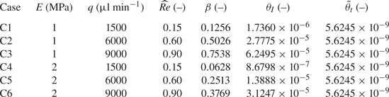
Similar to the experiments of Verma & Kumaran (Reference Verma and Kumaran2013), cases C1 to C3 and C4 to C6 summarized in table 5 are each based on a single microchannel, operated under different flow conditions. As catalogued in table 6, the steady and dynamic responses of the new 1-D FSI model match several experimental observations qualitatively, which indicates that the proposed model can provide unique insights into this unstable FSI problem. However, we cannot perform direct quantitative comparisons between our 1-D model and the experiments of Verma & Kumaran (Reference Verma and Kumaran2013), for the following reasons. First, the experiments’ soft wall was compressed upon a rigid outer surface, unlike our model wherein we have a soft wall that bulges outwards in an unconstrained manner (being stress-free on its outer surface). Further, in the experiments, the wall thickness was comparable to the channel's width, with two sidewalls made rigid. Consequently, the deformation field within the compliant wall in the microchannels fabricated by Verma & Kumaran (Reference Verma and Kumaran2013) is described by a different leading-order theory of the flow-induced deformation than the theories considered herein (recall § 4). At this time, it is not clear whether an exact solution (along the lines of Wang & Christov (Reference Wang and Christov2019)) could be obtained for the deformation in the configuration fabricated by Verma & Kumaran (Reference Verma and Kumaran2013). The main difference would be in the definition of  $\beta$. Nevertheless, since the experiments did consider long and shallow microchannels with a slender deformable wall, the assumptions made in §§ 3 and 4 apply. Therefore, the FSI physics in these experiments are expected to be captured by the theoretical framework proposed herein. Indeed, as discussed by Verma & Kumaran (Reference Verma and Kumaran2013), the FSI-induced instabilities are generic, thus are not expected to be an ‘accidental’ phenomenon occurring only in some specific experimental devices. It follows that our qualitative comparisons below are meaningful and useful for validating the proposed 1-D FSI model.
Table 6. Qualitative comparison between the experimental observations of Verma & Kumaran (Reference Verma and Kumaran2013) and the predictions of the proposed global 1-D FSI model.
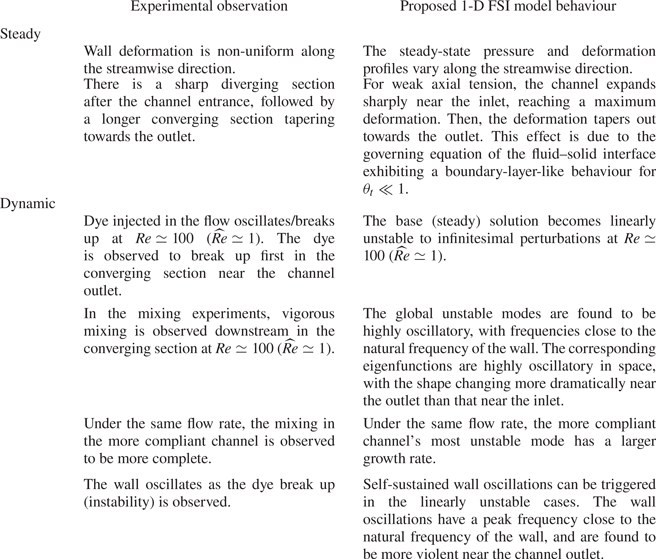
6. Base state: features of the inflated microchannel at steady state
At steady state, all the time derivatives vanish. From (5.3a), we have  $Q\equiv 1$, upon imposing the fixed-flux upstream boundary condition from (5.4a). The remaining (4.9), (4.7) and (5.3b), together with the unsatisfied boundary condition (5.4b) and (5.5), constitute a nonlinear two-point boundary value problem (Keller Reference Keller1976). This nonlinear system is solved using the newton_krylov routine from the SciPy stack (Virtanen et al. Reference Virtanen2020), following the procedure described in the supplementary material and movies available at https://doi.org/10.1017/jfm.2022.802.
Also, note that (4.9), (4.7) and (5.3b) can be combined to form a single equation, in terms of the steady-state deformed height  $\bar {H}_0$, written as
 \begin{equation} \frac{6}{5}\widehat{Re}\frac{1}{\bar{H}_0^{3}}\frac{\mathrm{d} \bar{H}_0}{\mathrm{d} Z} = \frac{1}{\beta}\left(\frac{\mathrm{d}\bar{H}_0}{\mathrm{d} Z}-\theta_t\frac{\mathrm{d}^{3}\bar{H}_0}{\mathrm{d} Z^{3}}\right)+ \frac{12}{\bar{H}_0^{3}}. \end{equation}
The boundary conditions for this third-order nonlinear ordinary differential equation are
 \begin{equation} \bar{H}_0(Z=0) = \bar{H}_0(Z=1)=1, \quad \left.\frac{\mathrm{d}^{2}\bar{H}_0}{\mathrm{d} Z^{2}}\right|_{Z=1}=0, \end{equation}
which correspond to zero displacement imposed at  $Z=0,1$, along with the gauge-pressure boundary condition at the outlet.
The steady responses of the exemplar cases from table 5 are shown in figure 2. The non-uniform deformation of the channel height is shown in figure 2(a), along with a zoom-in view near the inlet given in figure 2(c). The channel inflates more for larger flow rates and/or for softer walls (i.e. with smaller  $E$). For each case, there is a sharp diverging section near the channel inlet, and a much longer converging section connecting to the channel outlet, which agrees with the experimental observations of Verma & Kumaran (Reference Verma and Kumaran2013). As for the pressure distribution, figure 2(b) shows that the compliance of the wall leads to a non-uniform pressure gradient so that the pressure varies nonlinearly with $z$. Furthermore, compared with the case of flow in a rigid channel, the total pressure drop is reduced significantly due to the expanded cross-sectional area resulting from the deformation of the wall. This phenomenon has been addressed and analysed, considering different geometrical configurations and elastic response, but typically limited to the case of $\widehat {Re}\to 0$ (see, e.g. Christov Reference Christov2022). However, our proposed 1-D FSI model pushes the limit to $\widehat {Re} = O(1)$. Figure 2(d) also zooms into the neighbourhood of the channel inlet. As the flow rate increases, a small region of positive pressure gradient appears. The reason for this effect is that, the sharp expansion of the channel's cross-section near the inlet makes the local velocity drop quickly (recall that $Q\equiv 1$ at steady state), and the positive pressure gradient aids in the deceleration of the flow (Inamdar et al. Reference Inamdar, Wang and Christov2020; Wang & Christov Reference Wang and Christov2021). Finally, the deformation-induced weak tension coefficients of the exemplar cases are shown in figure 2(e). We observe that $\theta _t$ increases as the flow rate increases because higher flow rates induce larger deformations. Moreover, for the same flow conditions, it is observed that $\theta _t$ is larger when the wall is more compliant.
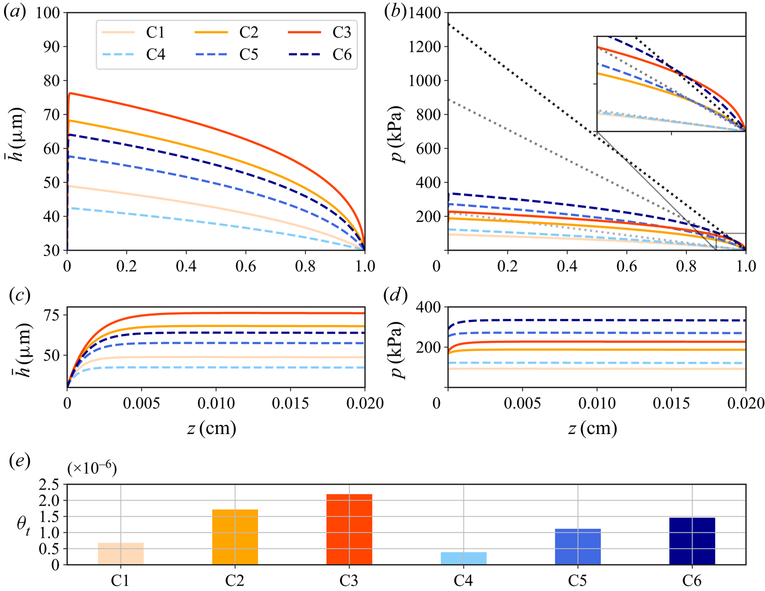
Figure 2. The steady-state response for the exemplar cases from table 5, for flow rates for  $q = 1500$, $6000$, $9000\ \mathrm {\mu }$l min $^{-1}$ (higher $q$ corresponds to darker curves). (a) The variation of the deformed channel height along $z$. (b) The pressure distribution along $z$, with the inset window showing a zoom-in view near the $z=\ell$. The dotted lines show the Hagen–Poiseuille law for a rigid channel (linearly variation for $p$ along $z$). Panels (c) and (d) show zoomed-in views for $\bar {h}$ and $p$ near the inlet, $z=0$, respectively. (e) The computed $\theta _t$ of the exemplar cases from table 5.
Next, to address the effect of  $\widehat {Re}$ and $\theta _t$, we compare the numerical results of the current 1-D FSI model with previous reported analytical results. At this stage, $\theta _t$ is fixed to be the corresponding values from figure 2(e). First, taking $\widehat {Re}\to 0$ and neglecting $\theta _t$, the pressure distribution and the deformation at steady state (Wang & Christov Reference Wang and Christov2021) are
 \begin{equation} P_0(Z)=\frac{1}{\beta}\{ [48\beta(1-Z)+1]^{1/4}-1 \}, \quad \bar{H}_0(Z) = 1+\beta P_0(Z). \end{equation}
Equation (6.3a,b) is the essentially the same as the model proposed by Gervais et al. (Reference Gervais, El-Ali, Günther and Jensen2006). However, in the current theoretical framework,  $\beta$ is obtained by solving an appropriate linear elasticity problem, instead of being calibrated by an experiment. Second, if only $\theta _t$ is neglected but $\widehat {Re} = O(1)$, the steady-state pressure distribution (Wang & Christov Reference Wang and Christov2021) is
 \begin{align} &P_0(Z)[ 1+\tfrac{3}{2}\beta P_0(Z)+ \beta^{2}P_0^{2}(Z) + \tfrac{1}{4}\beta^{3} P_0^{3}(Z) - \tfrac{6}{5}\widehat{Re}\beta]=12(1-Z),\nonumber\\ &\quad \quad \bar{H}_0(Z) = 1+\beta P_0(Z). \end{align}
Observe that (6.4a,b) reduce to (6.3a,b) for  $\widehat {Re}\to 0$. Finally, we mention that if both $\theta _t,\widehat {Re}\ne 0$, (6.1) is essentially a singular perturbation problem, which can be solved using the method of matched asymptotic expansions. Specifically, Wang & Christov (Reference Wang and Christov2021) showed that there exists a boundary layer near $Z=0$ of thickness $O(\theta _t^{1/2})$, and obtained a matched asymptotic solution, which is too lengthy to summarize here.
In figure 3, we show a comparison between the steady-state solution obtained by numerical simulation of the 1-D FSI model and the analytical results mentioned above. For a low flow rate, with  $\widehat {Re}=0.15$, the fluid inertia is not important, thus the numerical results agree well with the analytical results, except near the inlet. In contrast, for a high flow rate, with $\widehat {Re}=0.9$, the results neglecting the effect of $\widehat {Re}$ (based on (6.3a,b)) tend to underestimate the channel deformation and the pressure distribution. Since (6.3a,b) and (6.4a,b) do not take into account the weak tension effect, the no-displacement restriction at the inlet is not satisfied. With $\theta _t$ included, whether the flow rate is low or high, a short diverging section of the channel height emerges near the inlet, indicating the feature of a boundary layer problem, as described above.
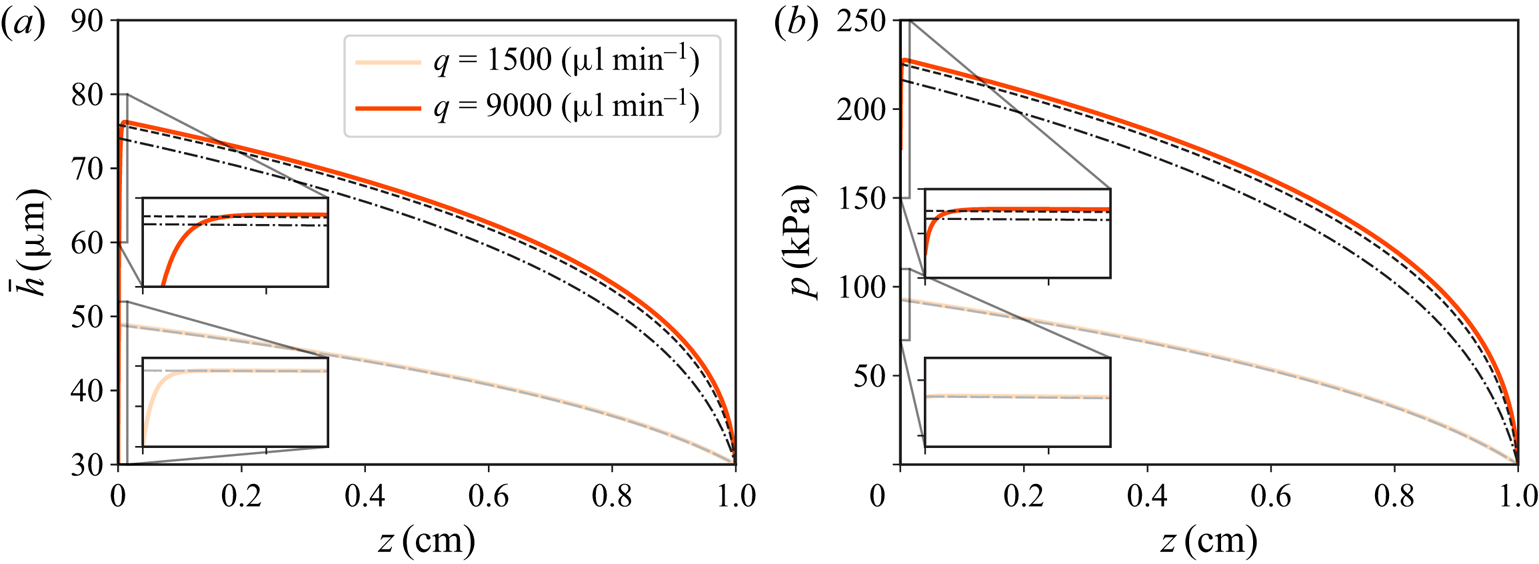
Figure 3. Comparison between the numerical solutions of the proposed 1-D FSI model and previously reported analytical results for the exemplar cases of C1 and C3. (a) The deformed channel height along  $z$. (b) The pressure distribution along $z$. The solid curves represent the numerical simulation of the 1-D FSI model at steady state. The dash–dotted curves represent the results calculated by (6.3a,b) with $\widehat {Re} = 0$ and $\theta _t = 0$. The dashed curves are calculated from (6.4a,b), in which $\theta _t = 0$ but $\widehat{Re}\ne 0$.
7. Linear stability of the inflated base state
In this section, we address the linear stability of the base (steady-state) solutions obtained in § 6. We have shown, in figure 2, that both the deformation and the pressure gradient are non-uniform along  $z$ in the inflated (non-flat) base state. This observation makes the linear stability problem non-trivial, as the linearized operators have variable coefficients and are not self-adjoint. The key question that this section will address is: Is the non-flat base state linearly stable to infinitesimal perturbations?
To answer this question, we perturb the base state with an infinitesimal disturbance as
 \begin{equation} Q(Z,T) = Q_0+\alpha \hat{Q}(Z,T), \quad \bar{H}(Z,T)=\bar{H}_0(Z) + \alpha \hat{H}(Z,T), \end{equation}
with  $\alpha \ll 1$. Note $Q_0=1$ for fixed flux upstream. Substituting the above into the governing equations (5.3) and (4.9), and keeping terms up to $O(\alpha )$, we obtain the following linear evolution equations:
 \begin{align} &\frac{\partial \hat{H}}{\partial T} +\frac{\partial \hat{Q}}{\partial Z} = 0,\end{align}
 \begin{align} &\frac{\widehat{Re}\beta}{\bar{H}_0}\frac{\partial\hat{Q}}{\partial T} + \frac{6}{5}\widehat{Re}\beta\left[\left(\frac{3Q_0^{2}}{\bar{H}_0^{4}}\frac{\mathrm{d} \bar{H}_0}{\mathrm{d} Z}-\frac{Q_0^{2}}{\bar{H}_0^{3}}\frac{\partial}{\partial Z}\right) \hat{H} +\left(-\frac{2Q_0}{\bar{H}_0^{3}}\frac{\mathrm{d} \bar{H}_0}{\mathrm{d} Z}+\frac{2Q_0}{\bar{H}_0^{2}}\frac{\partial}{\partial Z}\right)\hat{Q}\right] \nonumber\\ &\quad +\theta_I\frac{\partial^{3} \hat{H}}{\partial Z\partial T^{2}} +\frac{\partial \hat{H}}{\partial Z}-\theta_t\frac{\partial^{3} \hat{H}}{\partial Z^{3}} + 12\beta\left(\frac{\hat{Q}}{\bar{H}_0^{3}}-\frac{3Q_0}{\bar{H}_0^{4}} \hat{H}\right)= 0. \end{align}
We further note that  $\theta _t$ in the above equation is fixed to be the steady-state value rather than computed from (4.13), i.e. we have neglected any modifications of $\theta _t$ introduced by the initial perturbations. It can be shown (see § 8.1) that this effect is negligible.
In this work, we only consider the asymptotic behaviour of infinitesimal initial perturbations, i.e. the modal analysis. To this end, we write
 \begin{equation} \hat{Q}(Z,T) =\tilde{Q}(Z)\, {\rm e}^{-\mathrm{i} \omega_G T}, \quad \hat{H}(Z,T)=\tilde{H}(Z)\, {\rm e}^{-\mathrm{i} \omega_G T}. \end{equation}
Since the base state is non-flat, the eigenfunctions  $\tilde {Q}$ and $\tilde {H}$ are not homogeneous in $Z$. Then, $\omega _G\in \mathbb {C}$ denotes the ‘global’ growth/decay rate of the eigenmode (Huerre & Monkewitz Reference Huerre and Monkewitz1990).
For computational convenience, (7.2) is rewritten in matrix form as
 \begin{equation} \underbrace{
\begin{pmatrix} 0 & \dfrac{\mathrm{d}}{\mathrm{d} Z} \\
\mathscr{L}_H & \mathscr{L}_Q
\end{pmatrix}}_{\boldsymbol{\mathsf{A}}} \underbrace{\begin{pmatrix}
\tilde{H} \\ \tilde{Q}\end{pmatrix}}_{\boldsymbol{\psi}} =
\mathrm{i} \omega_G \underbrace{ \begin{pmatrix} 1 & 0\\ 0
&
\dfrac{\widehat{Re}\beta}{\bar{H}_0}-\theta_I\dfrac{\mathrm{d}^{2}}{\mathrm{d}
Z^{2}} \end{pmatrix}}_{\boldsymbol{\mathsf{B}}}
\underbrace{\begin{pmatrix} \tilde{H} \\
\tilde{Q}\end{pmatrix}}_{\boldsymbol{\psi}},
\end{equation}
\begin{equation} \underbrace{
\begin{pmatrix} 0 & \dfrac{\mathrm{d}}{\mathrm{d} Z} \\
\mathscr{L}_H & \mathscr{L}_Q
\end{pmatrix}}_{\boldsymbol{\mathsf{A}}} \underbrace{\begin{pmatrix}
\tilde{H} \\ \tilde{Q}\end{pmatrix}}_{\boldsymbol{\psi}} =
\mathrm{i} \omega_G \underbrace{ \begin{pmatrix} 1 & 0\\ 0
&
\dfrac{\widehat{Re}\beta}{\bar{H}_0}-\theta_I\dfrac{\mathrm{d}^{2}}{\mathrm{d}
Z^{2}} \end{pmatrix}}_{\boldsymbol{\mathsf{B}}}
\underbrace{\begin{pmatrix} \tilde{H} \\
\tilde{Q}\end{pmatrix}}_{\boldsymbol{\psi}},
\end{equation}
with the operators  $\mathscr {L}_H$ and $\mathscr {L}_Q$ defined as
 \begin{align} \mathscr{L}_H &= \frac{6}{5}\widehat{Re}\beta \left(\frac{3Q_0^{2}}{\bar{H}_0^{4}}\frac{\mathrm{d} \bar{H}_0}{\mathrm{d} Z}- \frac{Q_0^{2}}{\bar{H}_0^{3}}\frac{\mathrm{d}}{\mathrm{d} Z}\right)+ \frac{\mathrm{d}}{\mathrm{d} Z}-\theta_t\frac{\mathrm{d}^{3} }{\mathrm{d} Z^{3}} -\frac{36\beta Q_0}{\bar{H}_0^{4}}, \end{align}
 \begin{align}\mathscr{L}_Q &= \frac{6}{5}\widehat{Re}\beta\left(-\frac{2Q_0}{\bar{H}_0^{3}} \frac{\mathrm{d} \bar{H}_0}{\mathrm{d} Z}+\frac{2Q_0}{\bar{H}_0^{2}} \frac{\mathrm{d}}{\mathrm{d} Z}\right) + \frac{12\beta}{\bar{H}_0^{3}}. \end{align}
Note that  $\mathscr {L}_H$ and $\mathscr {L}_Q$ are linear operators with non-constant coefficients, as a consequence of the non-flat base state. Also note in $\boldsymbol{\mathsf{B}}$, $\theta _I \mathrm {d}^{2}\tilde {Q}/\mathrm {d} Z^{2}$ originates from $\theta _I\partial ^{3} \hat {H}/\partial Z\partial T^{2} = \theta _I \partial ^{3} \hat {Q}/\partial Z^{2}\partial T$, using (7.2a).
Since the base state has satisfied all the boundary conditions from (5.4a,b) and (5.5). The boundary conditions for the infinitesimal perturbations are homogeneous:
 \begin{gather} \tilde{Q}|_{Z=0}=\left.\frac{\mathrm{d} \tilde{Q}}{\mathrm{d} Z}\right|_{Z=0}= \left.\frac{\mathrm{d} \tilde{Q}}{\mathrm{d} Z}\right|_{Z=1}=0, \end{gather}
 \begin{gather}\tilde{H}|_{Z=0}=\tilde{H}|_{Z=1}=\left.\frac{\mathrm{d}^{2} \tilde{H}}{\mathrm{d} Z^{2}}\right|_{Z=1}=0. \end{gather}
The first boundary condition is deduced from the fixed flux upstream boundary condition, while the boundary conditions in terms of  $\tilde {H}$ correspond to the no-displacement restrictions at both ends and the outlet pressure set to gauge. The remaining two boundary conditions on $\tilde {Q}$ are derived from the (5.3a) by imposing zero displacement at the channel inlet and outlet.
Equation (7.4) subject to (7.6) gives rise to a generalized eigenvalue problem, which can be solved numerically using the Chebyshev pseudospectral method (see the supplementary material and movies for details). For all the eigenmodes resolved, if the corresponding  $\textrm{Im}(\omega _G)>0$, we say the non-flat base state of the 1-D FSI system is linearly unstable to infinitesimal disturbances.
7.1. Eigenspectra of the exemplar cases
Here, it is illustrative to plot dimensional quantities to show how a corresponding physical system would behave. To this end, we write the dimensional frequency as
 \begin{equation} f_g = \frac{\omega_G}{2{\rm \pi} \mathcal{T}_f} = \frac{\omega_G q}{2{\rm \pi} \ell w h_0}. \end{equation}
Note that  $f_g\in \mathbb {C}$, such that $\textrm{Re} (f_g)$ is the oscillatory frequency of the corresponding eigenmode, i.e. $[\tilde {H}, \tilde {Q}]^{T}$ in our formulation, while $\textrm{Im}(f_g)$ is the eigenmode's growth/decay time constant.
On the other hand, since (4.9) essentially represents a mechanical oscillator, the dimensionless and dimensional natural frequency of the oscillator, denoted as  $F_N$ and $f_n$, respectively, can be approximated as
 \begin{equation} F_N \approx \frac{1}{2{\rm \pi} \sqrt{\theta_I}}, \quad f_n \approx \frac{F_N}{\mathcal{T}_f} = \frac{F_N q}{\ell w h_0}. \end{equation}
Unlike  $f_g$, both $F_N,f_n\in \mathbb {R}$. Also note that, (7.8a,b) do not take the tension effect into account, but since tension is weak, we believe (7.8a,b) provide a good approximation to the natural frequency of the system.
In figure 4, we show the calculated eigenspectra for the six exemplar cases from table 5. First, observe that the eigenspectra are symmetric about the imaginary axis in the complex plane. This symmetry is a consequence of the formulation of the generalized eigenvalue problem (see (7.4)), as the matrix  $\boldsymbol{\mathsf{A}}$ on the left-hand side is purely real, while the matrix $\mathrm {i}\boldsymbol{\mathsf{B}}$ on the right-hand side is purely imaginary. This symmetry is also a feature of the eigenvalue analyses in Inamdar et al. (Reference Inamdar, Wang and Christov2020) and Wang & Christov (Reference Wang and Christov2020).
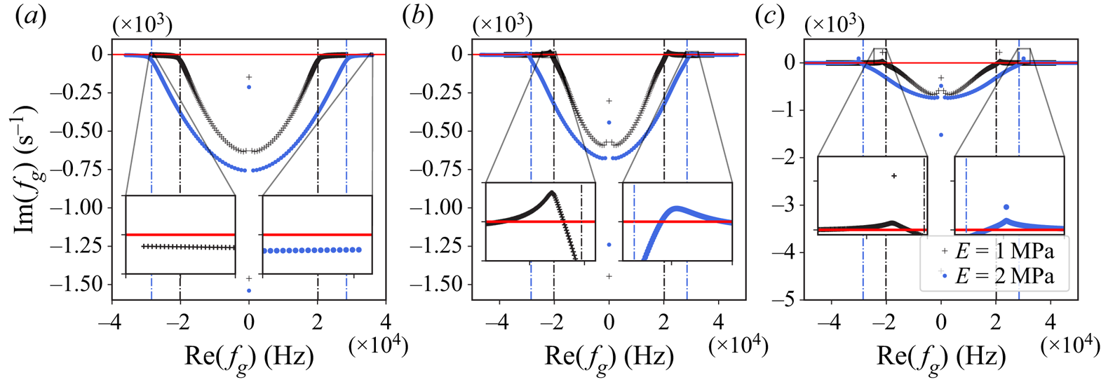
Figure 4. Eigenspectra of the exemplar cases from table 5: (a)  $q=1500\ \mathrm {\mu }$l min $^{-1}$ (C1 and C4); (b) $q=6000\ \mathrm {\mu }$l min $^{-1}$ (C2 and C5); (c) $q=9000\ \mathrm {\mu }$l min $^{-1}$ (C3 and C6). The symbols represent the discrete eigenvalues for $E=1$ MPa and $E=2$ MPa, respectively. The red horizontal line mark the position of real axis, i.e. $\textrm{Im}(f_g)=0$. The dash–dotted lines mark the natural frequencies calculated by (7.8b). The insets in each panel have the same vertical axes.
Second, the 1-D FSI system transitions from stability (figure 4a) to instability (figures 4b and 4c) as the flow rate is increased. The fluid inertia becomes more prominent as the flow rate is increased, indicated by the magnitude of  $\widehat {Re}$, which is associated with the nonlinear terms on the left-hand side of (5.3b). For the six exemplar cases from table 5, we observe that the linear instability typically occurs for $\widehat {Re}\simeq 1$, or equivalently $Re\simeq 100$, which is close to the values reported for the microchannel experiments showing instability (Verma & Kumaran Reference Verma and Kumaran2013).
Third, it is observed that the unstable regions in figures 4(b) and 4(c) are close to the natural frequency, indicating that the instabilities are related to the resonance of the wall. Due to the weak solid inertia, the natural frequency calculated from (7.8b), as well as  $\textrm{Re} (f_g)$ in the unstable region, is as high as $\simeq 10^{4}$ Hz. This fact also matches the local linear stability analysis of Verma & Kumaran (Reference Verma and Kumaran2013), who reported that the least stable mode oscillates at a frequency of the order of $10^{4}$ Hz. Moreover, one of the common features of the eigenspectra in figure 4 is that, away from the unstable region $\textrm{Im}(f_g)\to 0^{-}$ as $|\textrm{Re} (f_g)|$ becomes large. This observation indicates that, apart from those modes that grow for the given flow conditions, the stable modes that oscillate with higher frequency decay slowly, which highlights the computational stiffness of the 1-D FSI system.
Lastly, the compliance of the wall does influence the shape of the eigenspectra. Since the stiffer wall has a larger natural frequency, its unstable region is located at higher frequencies than its softer counterpart. Note that in figure 4, the two zoom-in insets in each panel have the same range for their vertical axes. Then it can be shown that the more compliant wall has the larger growth rate (or the smaller decay rate in the linearly stable case) for the least stable mode, which could be related to the experimental observations that the softer microchannel is more prone to instabilities (Verma & Kumaran Reference Verma and Kumaran2013).
Since both  $\theta _I$ and $\theta _t$ are small quantities in the solid mechanics (4.9), it is informative to show a comparison of the linear stability between cases either with $\theta _I=0$ or $\theta _t=0$. We consider three different such cases: (i) $\theta _I\ll 1$ and $\theta _t\ll 1$; (ii) $\theta _I = 0$ and $\theta _t\ll 1$; (iii) $\theta _I=0$ and $\theta _t=0$. The base states of both cases (i) and (ii) are the same, governed by (6.1). However, in case (iii), the system cannot satisfy $\bar {H}(0)=0$, thus the corresponding base state should be taken from (6.4a,b). As shown in figure 5(a), we observe that even though the solid inertia and tension are weak in the system, the inclusion of these weak effects changes the eigenspectrum fundamentally. The non-flat base state from (6.4a,b) is shown to be linearly stable. With only $\theta _t\ne 0$, case (ii) can predict linear stability only while case (i) with both $\theta _I,\theta _t\ne 0$ is linearly unstable. Furthermore, as shown in both cases (ii) and (iii), for $\theta _I=0$, the eigenmodes oscillate with higher frequencies. The reason is that, in this case, the natural frequency $F_N \to \infty$ as $\theta _I\to 0$.
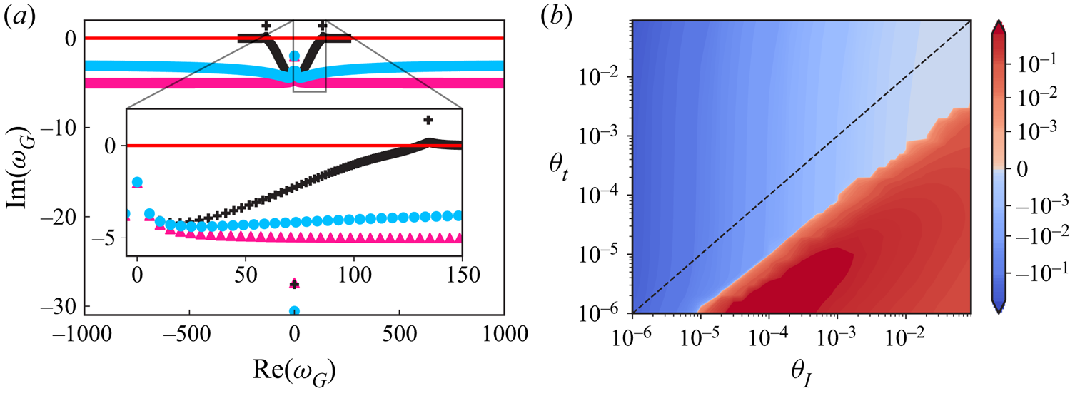
Figure 5. (a) Comparison of the eigenspectra of the case with  $\theta _I\ll 1$ and $\theta _t\ll 1$ (+), the case with $\theta _t\ll 1$ but $\theta _I=0$ ( $\bullet$, blue), and the case with $\theta _I=0$ and $\theta _t=0$ ( $\blacktriangle$, pink). The dimensionless parameters are taken as per case C3 in table 5. (b) Contour plot of $\textrm{Im}(\omega _G)$ of the least stable mode as a function of $\theta _I$ and $\theta _t$, with $\widehat {Re}$ and $\beta$ taken from case C3 in table 5. The dashed line marks $\theta _I = \theta _t$.
To further investigate the effect of  $\theta _I$ and $\theta _t$, we calculated the growth/decay rate of the least stable mode by taking different combinations of $\theta _I$ and $\theta _t$, fixing $\widehat {Re}$ and $\beta$ as the values corresponding to case C3. As shown in figure 5(b), for both $\theta _I$ and $\theta _t$ across five orders, linear instabilities are only observed when $\theta _I$ is at least one order larger than $\theta _t$. Since the dimensionless phase speed of the transverse waves along the fluid–solid interface is $\sqrt {\theta _t/\theta _I}$, then the linear instability occurs when the transverse waves propagate (much) slower than the flow.
7.2. Eigenfunctions of the exemplar cases
Each eigenvalue is associated with an eigenfunction pair, i.e.  $[\tilde {H}, \tilde {Q}]^{T}$ via (7.4). For the eigenvalues with larger $|\textrm{Re} (\omega _G)|$, the corresponding eigenfunctions are more oscillatory in space. For example, for the purely decay mode with $\textrm{Re} (\omega _G)=0$, the corresponding eigenfunctions are found to be purely real and non-oscillatory, as shown in figure 6. However, for the least stable modes of the linearly unstable cases from table 5, as shown in figure 7, with $|\textrm{Re}(\omega _G)|\gg 1$, the corresponding eigenfunctions are highly oscillatory in space. The corresponding eigenvalues for the eigenfunctions in figures 6 and 7 are tabulated in table 7.
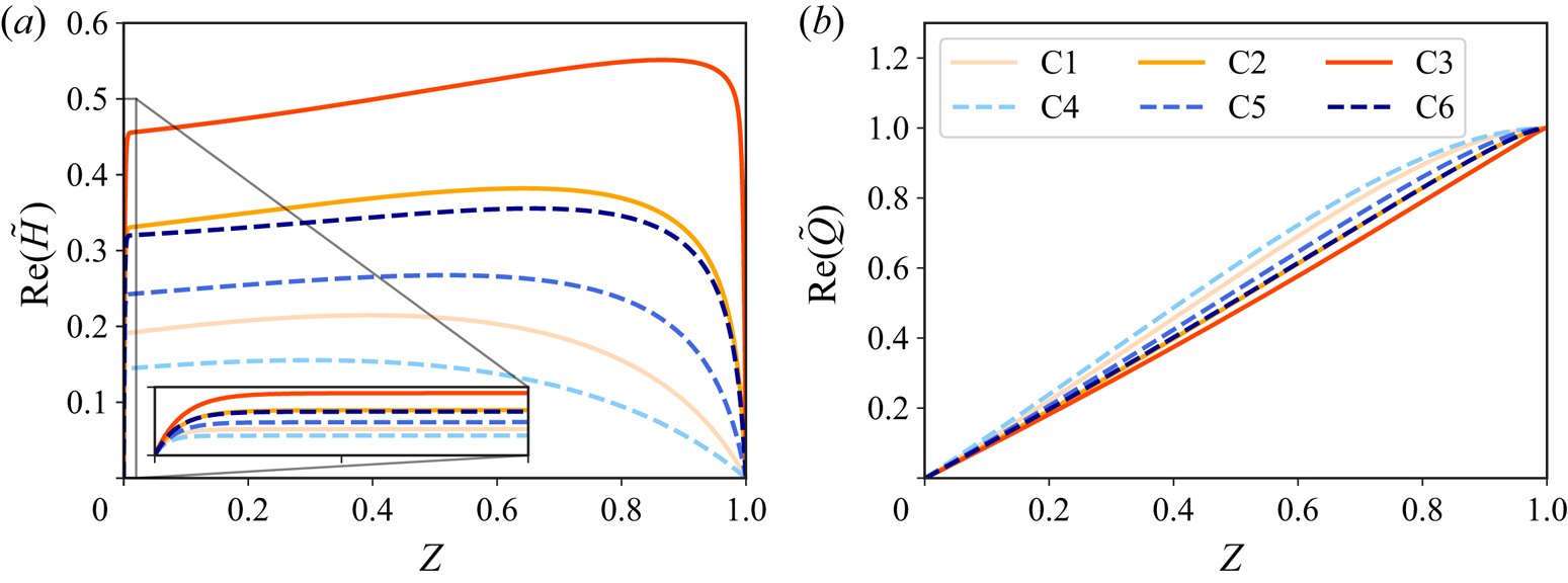
Figure 6. The eigenfunctions of the pure decay eigenmodes of the six exemplar cases from table 5. The eigenfunctions have been scaled such that  $\max |\tilde {Q}|=1$.
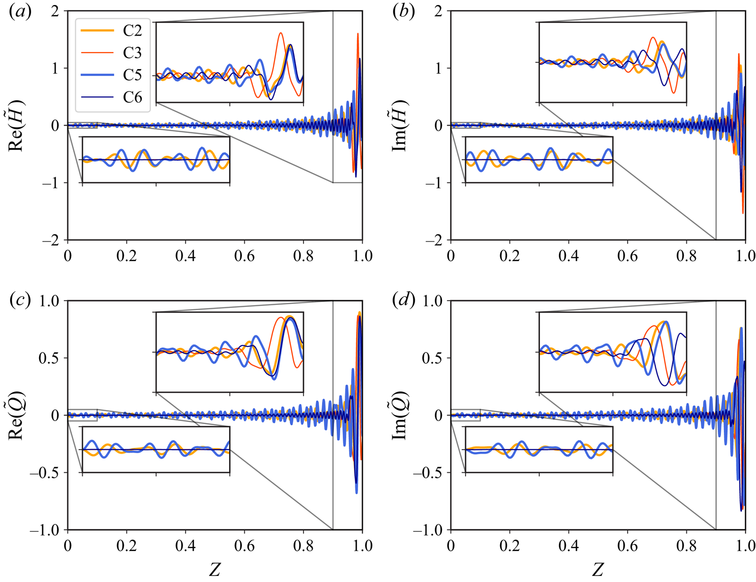
Figure 7. The eigenfunctions of the least stable modes for the linearly unstable cases, i.e. C2, C3, C5 and C6 in table 5. The eigenfunctions have been scaled such that  $\max |\tilde {Q}|=1$.
Table 7. The dimensionless eigenvalues,  $\omega _G$, for the pure decay modes and for the least stable modes of the exemplar cases from table 5.
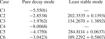
We do not tabulate the least stable modes of the linearly stable cases in table 7 because it is hard to pick out the least stable mode due to the limitation of the numerical method. In that case, we observe that the least stable mode is always the farthest eigenvalue away from the imaginary axis, if computed with the Chebyshev pseudospectral method using different number of Gauss–Lobatto points  $N$. In principle, there are an infinite number of eigenvalues in the 1-D FSI system, resolving all of which would require an infinite number of Gauss–Lobatto points. Unfortunately, $N$ cannot be arbitrarily large because matrices in (7.4) will become ill-conditioned.
Let us take a closer look at the eigenfunctions of the least stable modes in figure 7. For all the cases, both  $\tilde {H}$ and $\tilde {Q}$ exhibit large oscillations near the channel outlet ( $Z=1$), which echoes the experimental observation that the instabilities were always first observed near the outlet in the converging section of the microchannel (Verma & Kumaran Reference Verma and Kumaran2013). Furthermore, for a larger growth rate, the difference in oscillations between the outlet and the inlet is more prominent (comparing C2 and C3, or C5 and C6).
The wavy forms of the eigenfunctions in figure 7 further inspire us to conduct a Fourier transform in space for each case. We have used SciPy's fft routine with a Blackman window. The results are summarized in figure 8 and the abscissa represents the reciprocal of the dimensionless wavelength, denoted by  $\varLambda =\lambda /\ell$. Here, $\lambda$ is the dimensional wavelength. Interestingly, there are always two peaks for all the cases. The major peak is located at $1/\varLambda \simeq 100$, meaning the dominant wavelength is of the order of the channel height (recall $\ell /h_0\approx 333$). This observation could be related to the results of the local linear stability analysis of Verma & Kumaran (Reference Verma and Kumaran2013), who found that the most unstable modes have a wavelength comparable to the channel height.
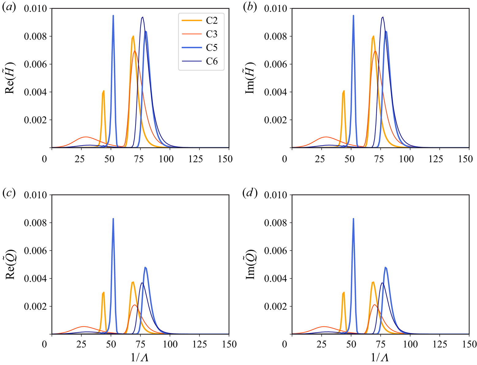
Figure 8. The spatial Fourier transform of the eigenfunctions from figure 7. Case C3 is scaled up by a factor of  $10$, while case C6 is scaled up a factor of $4$.
$4$.
8. Dynamic response of the microchannel
In this section, we solve the 1-D FSI model, by discretizing the governing equations in space and time, to investigate the dynamic responses. The spatial discretization is based on the Chebyshev pseudospectral method (Boyd Reference Boyd2000; Shen, Tang & Wang Reference Shen, Tang and Wang2011), while the ‘Newmark- $\beta$’ method (Subbaraj & Dokainish Reference Subbaraj and Dokainish1989) is used for the time integration; see the supplementary material and movies for further details about the numerical method and its benchmarking.
8.1. Evolution from a perturbed inflated state
First, to validate the linear stability results from § 7, at  $T=0$, we perturb the steady-state solution of the 1-D FSI model using the eigenfunction of a specific mode. Then, $\textrm{Im}(\omega _G)$ indicates the growth/decay rate of the perturbation, while $2{\rm \pi} /\textrm{Re}(\omega _G)$ is the period of the perturbation's oscillations.
The first example is the linearly stable case C1 ( $q=1500$ $\mathrm {\mu }$l min $^{-1}$) perturbed from the steady state with the eigenfunctions of the pure decay mode tabulated in table 7. The shapes of the corresponding eigenfunctions are shown in figure 6. The decay rate of the perturbation to the steady flow agrees well with the corresponding $\textrm{Im}(\omega _G)$, as shown in figure 9(a). No oscillations are observed in the evolution because $\textrm{Re}(\omega _G)=0$ in this case.
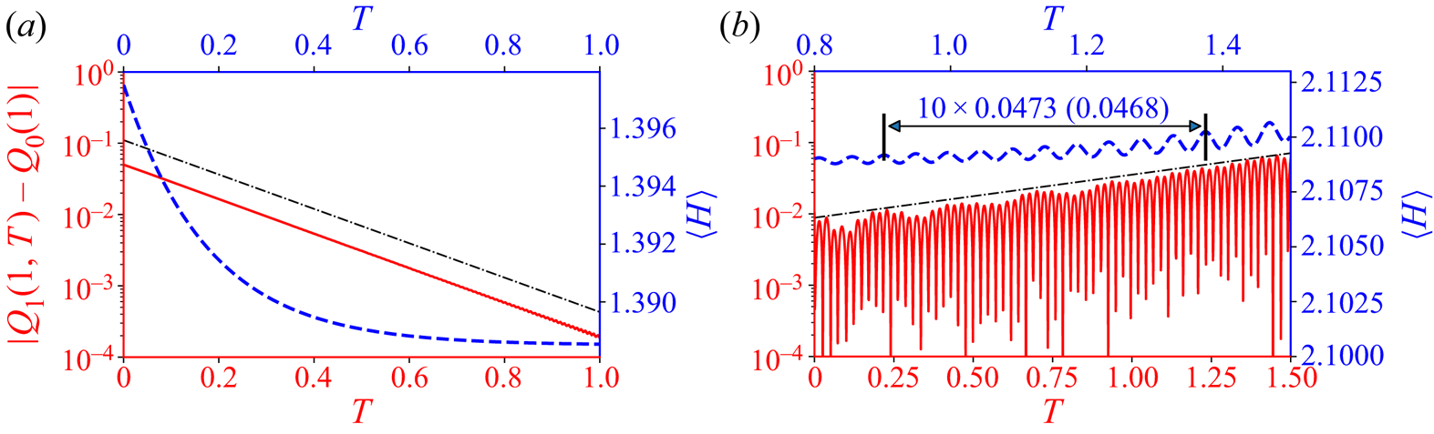
Figure 9. Time history of the difference between the instantaneous outlet flow rate and the steady one, i.e.  $|Q(1,T)-Q_0(1)|$ (solid, left-hand axes, also recall that $Q_0(Z)\equiv 1$ for the chosen boundary conditions), and the axially average deformed height, $\langle H\rangle (T) = \int _0^{1} \bar {H}(Z,T)\, \mathrm {d} Z$ (dashed, right-hand axes). (a) The steady state is perturbed using the eigenfunctions of the pure decay mode of case C1. (b) The steady state is perturbed using the eigenfunctions of the most unstable mode of case C3. The dot–dashed trendlines represent the growth/decay of perturbations, based on the imaginary part of the eigenvalues from table 7. In panel (b), the computed period of oscillation is marked. The value in parenthesis is from linear stability analysis, i.e. $2{\rm \pi} /\textrm{Re}(\omega _G)$.
The second example corresponds to the linearly unstable case C3. At  $T=0$, the steady state is perturbed by the eigenfunction of the corresponding most unstable mode. The shapes of the eigenfunctions are shown in figure 7, while the corresponding eigenvalues are given in table 7. Both the simulated growth rate and the oscillation period agree well with the linear stability analysis, as shown in figure 9(b). Here, note that the tension coefficient $\theta _t$ in (4.9) is estimated from the instantaneous wall deformation, thus it is time dependent. Meanwhile $\theta _t$ is fixed to be the steady-state value for the purposes of the linear stability analysis. The good agreement between the numerical simulation and the linear stability analysis indicates that neglecting the time dependence of $\theta _t$ for the linear stability analysis is valid. The actual simulations for each case are conducted for a longer time window. Interestingly, although the oscillations of the system are sustained, no saturated periodic state emerges during the course of the simulations. The simulations for cases C3 and C5 are available in Appendix B.
8.2. Evolution from a flat initial state
Starting the simulations with an undeformed channel initial condition (as in (5.6b)) would be more realistic of how a microfluidic device might be operated. With (5.6a,b) as the initial conditions, cases C1 and C4 are linearly stable and reach the steady state without detectable oscillations. The evolution of the representative quantities for case C4 are shown in figure SM.2 in the supplementary material and movies, wherein a video of the evolution under case C1 is also provided. In this subsection, we focus on the two linearly unstable cases C3 and C6. All of the results shown below have been verified by time step refinement (see the supplementary material and movies and figure SM.3 therein, for example).
First, the evolution of the outlet flow rate and the inlet pressure for cases C3 and C6 are shown in figure 10. In both cases, the outlet flow rate first decreases and then increases, reaching a value close to the imposed flow rate at late times. Meanwhile, the inlet pressure increases to a value slightly below the steady-state inlet pressure. Small-amplitude oscillations are observed in the evolution of both quantities. More importantly, the oscillations become magnified at later times in the simulation, which suggests that these unstable cases will not reach the steady state. It can be shown (by running longer-time simulations) the that these oscillations are not unbounded. Nevertheless, similar to the cases discussed in § 8.1, no saturated periodic state appears to emerge during the time window of the simulations shown in this subsection.

Figure 10. Time histories of the outlet flow rate and the inlet pressure for (a) case C3 and (b) case C6, respectively, with (5.6a,b) being the initial conditions. The dot–dashed lines mark the flow rate at steady state, while the dashed lines mark the inlet pressure at the steady state.
It is more enlightening to contrast the two simulations shown in figure 10. For these two cases, all system parameters are the same, except that Young's modulus for case C3 is half of that for case C6. With a more compliant wall, the instabilities under case C3 develop more quickly. Specifically, more ‘violent’ oscillations are observed in case C3 for the outlet flow rate and the inlet pressure than in case C6. These oscillation amplitudes could be, qualitatively, representative of the observations in dye-stream experiments. In other words, dye break up could be expected when more violent oscillations occur in softer channels, while the dye steam may just oscillate (without breaking up) if the channel is less compliant (thus, the oscillations in the flow rate and pressure are milder). Indeed, it was observed in the experiments that the dye breaks-up at lower  $Re$ in softer channels (Verma & Kumaran Reference Verma and Kumaran2013).
Next, let us take a closer look at the evolution of the fluid–solid interface. The example in figure 11 corresponds to case C3 in figure 10(a), while the evolution under case C6 is qualitatively similar. Initially, for  $0\leq t\leq 1\ {\rm ms}$ as shown in figure 11(a), the interface bulges near the channel inlet first because the pressure is relatively high there. At the same time, transverse waves are shed and propagate from the inlet to the outlet until they are reflected at the downstream boundary of the domain. There is a dramatic increase in the total volume of fluid in the channel at this stage. Thereafter, the deformation of the wall stops growing, but the transverse waves still propagate back and forth along the fluid–solid interface. Compared with figure 11(a), the transverse waves have smaller wavelength and amplitudes. Furthermore, the interface shape at this stage is close to the steady-state shape, as seen in figure 11(b). The deviation of the interface's dynamic deformation from the steady one is plotted for $4.0\ {\rm ms} \leq t\leq 6.5\ {\rm ms}$ in figure 11(c), where the wave propagation can be clearly observed. Interestingly, after a while, the oscillations near the channel's outlet continue to grow and become larger than the oscillations anywhere else along the channel, which explains why the variations of the outlet flow rate appear more prominent compared with those of the inlet pressure in figure 10. This observation is also corroborated by the experimental observation that the instabilities always initiate near the channel's outlet.

Figure 11. Evolution of the shape of the fluid–solid interface from the flat initial condition (5.6b) (movie available in the supplementary material and movies). (a) Shape of the interface for  $0 \leq t \leq 1$ ms. (b) Comparison of the interface shape at $t=3.5$ ms with the steady state. (c) Space–time plot of the difference between the instantaneous interface shape $\bar {u}_y$ and the steady state $\bar {u}_y^{s}$, i.e. $\bar {u}_y - \bar {u}_y^{s}$, for $4.0\ {\rm ms}\leq t \leq 6.5\ {\rm ms}$.
To better emphasize the difference in the wall motions near the inlet versus near the outlet, the vertical velocities of the fluid–solid interface at  $z=0.9\ell$ (near the outlet) and $z=0.1\ell$ (near the inlet) of case C3 are plotted in figure 12 (see the supplementary material and movies for the details of reconstructing the velocities). The three stages discussed in figure 11 can also be identified from the time histories of the vertical velocities shown in figure 12. At early times, since the wall bulges first near the channel inlet, the vertical velocity at $z=0.1\ell$ is larger. The motion at $z=0.9\ell$ starts after the transverse waves reach the channel outlet. In the intermediate stage, during which the channel volume does not change significantly, the oscillations at both positions remain relatively small, until the motion near the outlet becomes amplified and leads to a striking difference in the oscillatory amplitudes at the two positions.

Figure 12. (a) Time histories of the vertical velocity of the fluid–solid interface of case C3 at  $z=0.9\ell$ (near the outlet) and $z=0.1\ell$ (near the inlet), respectively. (b) Fourier transform of the corresponding time histories from (a). The dotted line marks the natural frequency calculated from (7.8b).
Figure 12(b) shows the corresponding time histories in the frequency (Fourier) domain. We observe that the peak is near the natural frequency of the wall (predicted by (7.8b)), indicating a resonant phenomenon. Due to the FSI, which gives rise to the transverse waves along the fluid–solid interface, the pressure oscillations exhibit a frequency close to the natural frequency of the wall as well, causing a feedback. Note that, the resonances are self-excited as no oscillatory components are introduced in the initial conditions (5.6a,b). Further, the oscillations are self-sustained as they do not die out during the entire simulation time window. Consequently, the demonstrated FSI-induced instabilities could be an effective and inexpensive way of enhancing mixing at the microscale.
9. Conclusion
We derived a new 1-D (reduced) FSI model for the physics underlying FSI-induced instabilities of flows conveyed in long and shallow microchannels with a deformable top wall. The key advance in our 1-D FSI model, compared with previous work, lies in the accurate modelling of the wall deformation due to two-way FSI. For collapsible tubes, a constant large tension is always included, though bending was also considered in some computational studies (Luo et al. Reference Luo, Cai, Li and Pedley2008; Liu et al. Reference Liu, Luo and Cai2012; Wang et al. Reference Wang, Luo and Stewart2021). Similarly, the 1-D FSI model of Inamdar et al. (Reference Inamdar, Wang and Christov2020) considered the top wall as a beam and took large-deformation-induced tension and bending into account. However, in a typical long and shallow rectangular microchannel, previous studies (Christov et al. Reference Christov, Cognet, Shidhore and Stone2018; Shidhore & Christov Reference Shidhore and Christov2018; Wang & Christov Reference Wang and Christov2019) have demonstrated that, under linear elasticity, at the leading order, the soft wall deforms more like a Winkler foundation with a variable stiffness (without assuming the Winkler model a priori or suffering from its limitations). In other words, the deformation of the channel's cross-section at different streamwise locations is fully determined by the local pressure. In contrast to previous 1-D models, the 1-D FSI model proposed herein maintains the dominance of the Winkler-foundation-like behaviour of the soft wall by modelling weak tension as a ‘boundary effect’ near the inlet of the channel. Moreover, the inertia of the solid is also modelled consistently, just like the inertia of the fluid being taken into account by lubrication theory at low, but finite, Reynolds number, extending the steady-state model in Wang & Christov (Reference Wang and Christov2021). Our proposed 1-D model establishes how the unsteady flow rate, the pressure and the channel deformation evolve together in a tightly coupled manner.
Importantly, we found that the predictions of the proposed 1-D FSI model agree qualitatively with key experiments (Verma & Kumaran Reference Verma and Kumaran2013) (summarized in table 6). Consequently, we believe that the present analysis leads to significant, novel insight into the experimentally observed low- $Re$ FSI-induced instabilities in compliant microchannels. In short, the physical insight provided by our new model is that FSI causes wall resonances, giving rise to self-sustained oscillations of the fluid–solid interface. These resonances are triggered thanks to the combined effect of weak axial tension and finite solid inertia, which leads to fluctuations in the local pressure at frequencies close to the natural frequency of the wall. Further, the experimentally observed dye break up (and ‘ultrafast’ mixing) are explained by the global instability of the non-flat (deformed) base state of our model, which was not accurately accounted for in previous work. Our proposed 1-D FSI model allows for the identification (computationally) of the critical conditions for instability of this coupled system. The predicted critical Reynolds number is in agreement with the value suggested by experiments.
To the experimentalist, our proposed 1-D FSI model provides a tool through which different microchannel designs can be rapidly prototyped and evaluated. Beyond that, our model provides a convenient way to evaluate operating conditions that might lead to instability and mixing. Extending the present results, the pressure drop could be prescribed across the channel (instead of fixing the flux at the inlet), similarly to the works of Stewart et al. (Reference Stewart, Waters and Jensen2009, Reference Stewart, Heil, Waters and Jensen2010). Further, the proposed 1-D modelling framework can be easily used to analyse soft conduits of different cross-sectional geometries and other boundary conditions, as long as the basic assumptions on the separation of scales (and weak versus dominant effects in the solid) are not violated.
The current work was motivated by microfluidic experiments and aimed to provide new qualitative and quantitative physical insights into these phenomena. Nevertheless, further work is needed to understand the full range of dynamic behaviours possible under the proposed 1-D FSI model. For example, in the linearly unstable case, the numerical simulations of the model using different time step sizes begin to diverge after a certain (long) integration time. This observation reminds us of the similarly chaotic behaviour observed in a 1-D FSI model derived by Jensen (Reference Jensen1992) in the somewhat different context of collapsible tubes. Similar to our 1-D FSI model, Jensen's model also exhibits multiple unstable modes, and its dynamics may be sensitive to initial conditions (due to the interactions of multiple unstable modes). Therefore, understanding the nonlinear dynamics of the proposed 1-D FSI model could be a fruitful avenue for future work. Further, since the observed oscillations are low-amplitude and high-frequency, asymptotic analysis could yield the stability boundaries (Jensen & Heil Reference Jensen and Heil2003). On the other hand, an Orr–Sommerfeld-type local stability analysis (similar to the Kumaran family of studies, recall § 1) could once again be conducted on the proposed model to complement to the global stability analysis. Investigating the connections between the local and global instabilities could provide insight regarding what types of excitations trigger unstable global modes (Stewart et al. Reference Stewart, Waters and Jensen2009, Reference Stewart, Heil, Waters and Jensen2010), opening the door towards more controllable ‘ultrafast mixing’ due to FSIs in compliant microchannels.
Supplementary material and movies
Supplementary material and movies are available at https://doi.org/10.1017/jfm.2022.802.
Acknowledgements
We thank E. Boyko for feedback on an earlier draft.
Funding
This work originates from research partially supported by the US National Science Foundation (NSF) under grant no. CBET-1705637. The manuscript was completed with partial support from NSF grant no. CMMI-2029540.
Declaration of interests
The authors report no conflict of interest.
Data availability statement
The data that support the findings of this study are openly available in the Purdue University Research Repository (PURR) at http://doi.org/10.4231/SX6D-1370.
Author contributions
X.W. led the analysis of the problem and the derivation of the mathematical model, to which also I.C.C. contributed. X.W. wrote the Python scripts and conducted all the case studies, numerical simulations and data analysis. Both authors contributed to the analysis of the data and conclusions drawn thereof. X.W. and I.C.C. jointly drafted and revised the manuscript for publication.
Appendix A. Modelling of weak deformation effects
A.1. Weak inertia and the effective interface thickness
The goal of previous studies was to find a solution for the fluid–solid interface displacement,  $\bar {u}_y$, from which to determine the cross-sectional area of the deformed fluidic channel. To illustrate this point, consider the microchannel studied by Wang & Christov (Reference Wang and Christov2019), which has a similar configuration to figure 1(a). In this case, the theory of the flow-induced deformation predicts that the vertical displacement of the solid, $U_Y^{s}= u_y^{s}(x,\hat {y},z) / \mathcal {U}_c$, varies with the vertical distance from the fluid–solid interface $(\hat {y}=0)$, as shown in figure 13. For the unsteady problem in this work, however, we must properly connect the motion of the fluid–solid interface to the non-uniform motion of the entire top wall. Since this variation is rapidly decaying, it is reasonable to expect that a suitable effective thickness of the fluid–solid interface, $b^{\star }$, can be introduced and used in (4.5). In doing so, the unsteady motion of the whole solid (of non-uniform vertical displacements) will be captured by the vertical motion of an interface of ‘virtual’ thickness $b^{\star }$.

Figure 13. Illustration of the displacement field in a thick wall predicted by (3.14) from Wang & Christov (Reference Wang and Christov2019). (a) Centreline displacement at  $x/w=X=0$ versus dimensionless vertical distance from the fluid–solid interface, $\hat {y}/w$. (b) Contour plot of the displacement field. Here, $\hat {y} = y+h_0$ and $\mathcal {U}_c = w\mathcal {P}_c/(h_0 \bar {E})$.
In analogy to the definition of the hydrodynamic boundary layer thickness (White Reference White2006; Panton Reference Panton2013), we define  $b^{\star }$ by requiring that the momentum of the solid wall's motion is equivalent to the momentum of the reduced interface's motion, i.e.
 \begin{equation} \rho_s \int_0^{d} \int_{{-}w/2}^{{+}w/2} \dot{u}^{s}_y(x,\hat{y},z) \,\mathrm{d}\kern0.06em x\,\mathrm{d}\hat{y} = \rho_s w b^{{\star}} \dot{\bar{u}}_y(z), \end{equation}
where the overdot denotes a time derivative. Since we have assumed that the solid deformation is governed by linear elasticity, the domain of integration is unchanged after deformation. Then, we can take the time derivative out of the integral, and consider an instantaneous balance. Substituting the definition of  $\bar {u}_y$, we obtain
 \begin{equation} b^{{\star}} = \frac{\displaystyle \int_0^{d} \int_{{-}w/2}^{{+}w/2} {u}_y^{s}(x,\hat{y},z) \,\mathrm{d}\kern0.06em x\,\mathrm{d}\hat{y}}{\displaystyle w \bar{u}_y} = \frac{\displaystyle \int_0^{d} \int_{{-}w/2}^{{+}w/2} {u}_y^{s}(x,\hat{y},z) \,\mathrm{d}\kern0.06em x\,\mathrm{d}\hat{y}}{\displaystyle \int_{{-}w/2}^{{+}w/2} {u}_y^{s}(x,0,z) \,\mathrm{d}\kern0.06em x}. \end{equation}
 Substituting equation (3.14) from Wang & Christov (Reference Wang and Christov2019) into (A2), we find that  $b^{\star }\approx 0.6141w$ for thick-walled microchannel ( $d^{2}/w^{2}\gg 1$). However, if the top wall is thin ( $d\simeq w$), plate theory can be invoked, and the midplane displacement can represent the bulk motion of the interface; in this case, $b^{\star } = d$.
A.2. Weak deformation-induced tension
Having introduced  $b^{\star }$, we are ready to give an expression for the weak tension, $\chi _t$. One possible scenario is that $\chi _t$ arises from the bulging of the wall. In principle, the deformation-induced tension is non-uniform along $z$. However, as mentioned, the variation of tension in $z$ is balanced with the shear stress in the flow, and thus can be neglected. Then, assuming the in-plane displacement (along $z$) is negligible, $\chi _t$ can be estimated by the average stretch of the wall (Hewitt et al. Reference Hewitt, Balmforth and De Bruyn2015), written as
 \begin{equation} \chi_t = \frac{Eb^{{\star}}}{\ell} \int_0^{\ell} \frac{1}{2}\left(\frac{\partial \bar{u}_y}{\partial z} \right)^{2} \, \mathrm{d} z. \end{equation}
Deformation-induced tension is expected to occur when the outlet of the channel is open to air, as in Gervais et al. (Reference Gervais, El-Ali, Günther and Jensen2006) and Verma & Kumaran (Reference Verma and Kumaran2013), or the pretension provided by external connectors is negligible. In the unsteady case,  $\chi _t$ is time-dependent.
Another possible situation is that the microchannel is prestretched and installed between an upstream and downstream section, as in the research on collapsible tubes mentioned in § 1. With the increase of the flow rate, the bulging of the wall is more prominent, leading to larger  $\chi _t$. However, beyond a certain flow rate, the deformation-induced tension will not be sufficient to hold the channel at the inlet and the outlet. In other words, the boundary conditions cannot be satisfied. The upper bound on the flow rate before the model breaks down is related to and found to increase with $\chi _t$ (Wang & Christov Reference Wang and Christov2021). Therefore, in this case when the deformation-induced tension is not sufficient, if the system is still to operate at such a high flow rate, external pretension needs to be provided. Nevertheless, for the validity of (4.5), the pretension in this case should be much larger than the deformation-induced tension. On the other hand, the third term in (4.5) needs to be small compared with the second term, to ensure the dominance of the Winkler-foundation-like mechanism.
Apart from weak tension, other elastic forces might also be relevant in other physical scenarios. For example, if the top wall is thin, bending could play a role. Another example comes from the elastic structures on top of thin fluid films, wherein (in addition to tension) bending and gravity are invoked to regularize the problem (see, e.g. Peng & Lister Reference Peng and Lister2020).
Appendix B. Long-time simulation of the evolution from a perturbed inflated state
The linear stability analysis only predicts the evolution of the perturbation in the vicinity of the steady state, i.e. for early times. The simulations in § 8.1 are actually conducted for a longer time window. The results for cases C3 and C5 are shown in figures 14 and 15, respectively. For the time window shown, the numerical results are verified by time step refinement. All representative quantities shown in figures 14 and 15 experience high-frequency oscillations with nonlinear variations in their amplitudes. No saturated (periodic) state is found in any of the cases. Actually, beyond the given time window, the simulation results diverge when using different time step sizes, which suggests that this nonlinear dynamical system may exhibit chaotic behaviour. However, pursing this possibility is beyond the scope of the present work. The most important conclusion from these simulations is that the perturbed steady state is unstable, and the system undergoes self-sustained oscillations, instead of returning to the inflated steady state.

Figure 14. Dynamic simulations of case C3, by perturbing the steady state with the eigenfunctions of the most unstable mode from table 7. (a) Time histories of representative quantities: the axially averaged deformed height; the inlet pressure and the axially averaged pressure; the outlet flow rate; and the vertical velocity of the interface at  $z=0.9$ cm and $z=0.1$ cm, respectively, from top to bottom. (b) Fourier transform of the time signals from (a). Note that in the second and fourth rows, the vertical axis has been rescaled for a clearer view. The dot–dashed lines mark $f_g$ and $2f_g$ (see (7.7)), while the dotted lines mark $f_n$ and $2f_n$ (see (7.8b)).

Figure 15. Dynamic simulations of case C5, by perturbing the steady state with the eigenfunctions of the most unstable mode from table 7. (a) Time histories of the representative quantities: the axially averaged deformed height; the inlet pressure and the axially averaged pressure; the outlet flow rate; and the vertical velocity of the interface at  $z=0.9$ cm and $z=0.1$ cm, respectively, from top to bottom. (b) Fourier transform of the time signals from (a). Note that in the second and fourth rows, the vertical axis has been rescaled to highlight the smaller-scale details. The dot–dashed lines mark $f_g$ and $2f_g$ (see (7.7)), while the dotted lines mark $f_n$ and $2f_n$ (see (7.8b)).
In figures 14 and 15, the axially averaged deformed height (first rows), the inlet pressure and the axially averaged pressure (second rows) are observed to vary in a small range ( $<1$
$<1$  $\mathrm {\mu }$m for the axially averaged deformation and $<10$ kPa for the pressure), which is consistent with the fact that no dramatic changes in the channel volume and the inlet pressure were reported in the experiments (Verma & Kumaran Reference Verma and Kumaran2013). On the contrary, the outlet flow rate (third rows) experiences more violent oscillations, which are prominent near the channel outlet, as shown in figure 7. In the fourth rows, the vertical velocity of the fluid–solid interface is shown. It is obtained via (5.1) and conservation of mass (see the supplementary material and movies for further details). Like the flow rate, the vertical velocity of the interface is observed to experience larger oscillatory amplitude near the channel outlet than that near the channel inlet, which again matches the experimental observation that the instabilities initiate near the channel's outlet.
Figures 14(b) and 15(b) show the Fourier transforms of the time histories of the corresponding representative quantity. It is observed that there is a peak near  $f_g$ (see (7.7)), showing a good agreement with the linear stability analysis. Also observe that $f_g$ is close to the natural frequency of the wall, $f_n$ (see (7.8b)), which indicates that the wall oscillations are a resonance phenomenon. Further, nonlinearity generates higher harmonics. In figure 14, there is another peak at $\approx 2f_g$, while in figure 15, the second peak is at a frequency higher than $2f_g$. The higher-frequency oscillations are more prominent near the channel inlet. For example, the second peak of the vertical velocity of the interface at $z=0.1$ cm is taller than the first peak. Furthermore, the higher-frequency oscillations in the inlet pressure are more prominent than the lower-frequency oscillations as shown in both figures 14 and 15.


 Open access