


1. Introduction
High-speed flows represent a challenging topic of interest for manifold configurations, including objects entering a planetary atmosphere or for atmospheric hypersonic flight (Gnoffo et al. Reference Gnoffo, Weilmuenster, Hamilton, Olynick and Venkatapathy1999). In such flows, conversion of massive amounts of kinetic energy into internal energy causes a sudden rise of the flow temperature. The effects triggered by the high temperatures include chemical reactions and vibrational relaxation phenomena on characteristic time scales comparable to the flow time scales. The complex thermochemical state induced by such conditions may affect quantities of interest for the design of high-speed vehicles significantly (Bertin & Cummings Reference Bertin and Cummings2006; Candler Reference Candler2019). In the past, thermochemical effects caused by hypersonic conditions have been investigated in more or less simple configurations. Most of the efforts focused on stagnation-point flows, of interest for bluff bodies re-entering the atmosphere (Fay & Riddell Reference Fay and Riddell1958; Armenise et al. Reference Armenise, Capitelli, Colonna and Gorse1996; Bonelli et al. Reference Bonelli, Tuttafesta, Colonna, Cutrone and Pascazio2017; Colonna, Bonelli & Pascazio Reference Colonna, Bonelli and Pascazio2019). In later stages of re-entry trajectories or for suborbital flight conditions characterized by higher free-stream densities, the flow description is further complicated by the transition from a laminar to a turbulent regime. Such a transition may be triggered by free-stream disturbances, erosion and ablation of the thermal protection systems (TPS) or due to surface defects, leading to sharp rise of the skin friction and heat fluxes at the walls. For this reasons, laminar-to-turbulent transition has been identified as a subject of major concern for the accurate prediction of the aerothermodynamic flow fields around objects flying at hypersonic speeds. A significant number of contributions in the literature have addressed the linear and nonlinear stability of flat-plate boundary layers in chemical non-equilibrium, sometimes up to the initial stages of transition. The pioneering studies of Malik & Anderson (Reference Malik and Anderson1991), Hudson, Chokani & Candler (Reference Hudson, Chokani and Candler1997) and Perraud et al. (Reference Perraud, Arnal, Dussillols and Thivet1999) pointed out that chemical reactions tend to promote the so-called second mode instability, similarly to strongly cooled walls. More recently, Marxen et al. (Reference Marxen, Magin, Shaqfeh and Iaccarino2013) and Marxen, Iaccarino & Magin (Reference Marxen, Iaccarino and Magin2014) used direct numerical simulations (DNS) to evaluate the maximum streamwise velocity disturbance caused by large- or small-amplitude waves in presence of chemical reactions. Kline, Chang & Li (Reference Kline, Chang and Li2019) and Knisely & Zhong (Reference Knisely and Zhong2019) investigated the effects of thermochemical non-equilibrium (TCNE) on boundary-layer stability; the effect of ablation has also been considered (Mortensen & Zhong Reference Mortensen and Zhong2016; Miró Miró & Pinna Reference Miró Miró and Pinna2021). On the other hand, while wall-bounded turbulence under low-enthalpy conditions (i.e. with air behaving as a calorically perfect gas) has been carefully scrutinized over the years, the interplay between TCNE conditions and turbulence has received much less attention. Compressible turbulent boundary-layer (TBL) configurations have been investigated with different turbulence injection techniques and wall treatments; for a thorough overview of DNS of TBLs at relatively low free-stream Mach numbers ( $M_\infty \leq 3$), the reader may refer to the work of Wenzel et al. (Reference Wenzel, Selent, Kloker and Rist2018) and references therein. Many efforts have been devoted to extending the validity of scaling laws derived for incompressible configurations (Morkovin Reference Morkovin1962) to compressible ones. Inspection of the hypersonic regime by means of high-fidelity simulations was initiated by the studies of Duan, Beekman & Martín (Reference Duan, Beekman and Martín2011), who performed DNS of temporally evolving TBLs with nominal free-stream Mach numbers up to 12 to prove the robustness of Morkovin's hypothesis even in high-speed flows. A DNS of a transitional spatially evolving boundary layer at Mach 6 was performed by Franko & Lele (Reference Franko and Lele2013), whereas Zhang, Duan & Choudhari (Reference Zhang, Duan and Choudhari2018) produced a database of cooled boundary layers up to $M_\infty =14$, with flow conditions representative of those encountered in hypervelocity wind tunnels. Huang et al. (Reference Huang, Nicholson, Duan, Choudhari and Bowersox2020) performed DNSs of zero-pressure-gradient hypersonic TBLs and conducted a priori and a posteriori analyses of the performances of different Reynolds-averaged Navier–Stokes (RANS) models. A handful of works focused on high-enthalpy flows, at free-stream conditions for which dissociation and recombination reactions are triggered (Martin & Candler Reference Martin and Candler2001; Duan & Martín Reference Duan and Martín2009). A comparative study between low- and high-enthalpy, reactive, temporally evolving boundary layers was performed by Duan & Martín (Reference Duan and Martín2011b); the authors found that the two closely resemble each other, since the scaling laws validated under low-enthalpy conditions still hold or could be generalized for high-enthalpy applications. The interaction of finite-rate chemistry with transitional and turbulent spatially developing boundary layers was recently investigated by Passiatore et al. (Reference Passiatore, Sciacovelli, Cinnella and Pascazio2021) and Di Renzo & Urzay (Reference Di Renzo and Urzay2021), who isolated the effects of chemical non-equilibrium on pseudo-adiabatic and cooled TBLs, respectively. In both studies, the effect of thermal non-equilibrium was neglected since the selected edge conditions were not expected to promote significant vibrational relaxation phenomena. The influence of these processes on turbulent flow behaviour has been investigated only for unconfined flow configurations so far, such as isotropic turbulence decay (Neville et al. Reference Neville, Nompelis, Subbareddy and Candler2014; Khurshid & Donzis Reference Khurshid and Donzis2019; Zheng et al. Reference Zheng, Wang, Noack, Li, Wan and Chen2020) and mixing layers (Neville et al. Reference Neville, Nompelis, Subbareddy and Candler2015; Fiévet et al. Reference Fiévet, Voelkel, Raman and Varghese2019).
The present work aims at bridging this knowledge gap with the investigation of a TBL exposed to both thermal and chemical non-equilibrium conditions. For that purpose, we perform a DNS of a flat-plate boundary layer, subjected to post-shock conditions of a  $6^{\circ }$ sharp wedge flying at Mach 20. The edge thermodynamic state is such that vibrational relaxation phenomena are significant within the boundary layer, while a mild chemical activity is developed.
The paper is organized as follows. The governing equations, the numerical method, the outline of the simulation and the main parameters are described in § 2. Numerical results are presented in § 3; focusing mostly on the fully turbulent regime, we illustrate the behaviour of the dynamic field and compare different transformations for the streamwise velocity. Afterwards, thermal non-equilibrium effects are inspected by highlighting the tight coupling with turbulent mixing mechanisms. Correlations deriving from the strong Reynolds analogy are also evaluated, as well as classical closures of the new terms arising in the RANS equations. Lastly, the coupling between compressibility effects and thermal non-equilibrium is investigated. Conclusions are then drawn in § 4.
2. Methodology
2.1. Governing equations and thermodynamic models
The fluid under investigation in the current study is air at high temperature, modelled as a five-species mixture of N $_2$, O $_2$, NO, O and N. When considering a gas under thermal non-equilibrium conditions, the vibrational energetic levels of the molecules in the mixture are partially excited and no longer equilibrated with the roto-translational ones. A direct consequence is that, even assuming that particle populations follow a Boltzmann distribution, the utilization of a single static temperature to represent all the energetic modes is no longer valid (Anderson Reference Anderson2006). A classical approach to deal with such conditions, referred to as multi-temperature in the literature, consists of taking into account the vibrational levels separately, by means of additional ‘vibrational’ temperatures for each molecule. In order to keep a reasonable number of equations to be integrated, the two-temperature model of Park (Reference Park1988) is adopted for the present calculations. Such a model, widely used in previous works (see, e.g. Hudson et al. Reference Hudson, Chokani and Candler1997; Franko, MacCormack & Lele Reference Franko, MacCormack and Lele2010; Bitter & Shepherd Reference Bitter and Shepherd2015), assumes that the vibrational energy states of each molecule satisfy a Boltzmann distribution characterized by only one vibrational temperature $T_{V}$, common to all diatomic species in the mixture (that is, N $_2$, O $_2$ and NO). A single additional conservation equation is, therefore, needed for the total vibrational energy $e_{V}$. Thus, the behaviour of such flows is governed by the compressible Navier–Stokes equations for multicomponent chemically reacting and thermally relaxing gases, which read
 \begin{gather} \frac{\partial \rho}{\partial t} + \frac{\partial \rho u_j }{\partial x_j} =0 \end{gather}
 \begin{gather}\frac{\partial \rho u_i}{\partial t} + \frac{\partial \left( \rho u_i u_j + p \delta_{ij} \right)}{\partial x_j} = \frac{\partial \tau_{ij}}{\partial x_j} \end{gather}
 \begin{gather}\frac{\partial \rho E}{\partial t} + \frac{\partial \left[\left(\rho E + p \right)u_j\right]}{\partial x_j} = \frac{\partial (u_i \tau_{ij})}{\partial x_j} - \frac{\partial (q^{{TR}}_j + q^{\text{V}}_j)}{\partial x_j} -\frac{\partial}{\partial x_j}\left(\sum_{n=1}^{NS} \rho_n u_{nj}^D h_n \right) \end{gather}
 \begin{gather}\frac{\partial \rho_n}{\partial t} + \frac{\partial \left( \rho_n u_j \right)}{\partial x_j} ={-}\frac{\partial \rho_n u_{nj}^D }{\partial x_j} + \dot{\omega}_n \quad (n = 1,..,{NS}-1) \end{gather}
 \begin{gather}\frac{\partial \rho e_{V}}{\partial t} + \frac{\partial \rho e_{V} u_j}{\partial x_j} = \frac{\partial}{\partial x_j} \left({-}q^{V}_j - \sum_{m=1}^{NM} \rho_m u_{mj}^D e_{{V}m} \right) + \sum_{m=1}^{{NM}} \left( Q_{{TV}m} + \dot{\omega}_m e_{{V}m} \right). \end{gather}
In the preceding formulation,  $\rho$ is the mixture density, $t$ the time coordinate, $x_j$ the space coordinate in the $j$th direction of a Cartesian coordinate system, with $u_j$ the velocity vector component in the same direction, $p$ is the pressure, $\delta _{ij}$ the Kronecker symbol and $\tau _{ij}$ the viscous stress tensor, modelled as
 \begin{equation} \tau_{ij} = \mu\left(\frac{\partial u_i}{\partial x_j} + \frac{\partial u_j}{\partial x_i} \right) -\frac{2}{3}\mu\frac{\partial u_k}{\partial x_k}\delta_{ij}, \end{equation}
with  $\mu$ the mixture dynamic viscosity. In (2.3), $E = e + \frac {1}{2}u_i u_i$ is the specific total energy (with $e$ the mixture internal energy), $q^{TR}_j$ and $q^{V}_j$ the roto-translational and vibrational contributions to the heat flux, respectively; $u_{nj}^D$ denotes the diffusion velocity and $h_n$ the specific enthalpy for the $n$th species. In the species conservation equations (2.4), $\rho _n = \rho Y_n$ represents the $n$th species partial density ( $Y_n$ being the mass fraction) and $\dot {\omega }_n$ the rate of production of the $n$th species. The sum of the partial densities is equal to the mixture density $\rho =\sum _{n=1}^{NS} \rho _n$, $NS$ being the total number of species. To ensure total mass conservation, the mixture density and $NS-1$ species conservation equations are solved, while the partial density of the $NS$th species is computed as $\rho _{NS} = \rho - \sum _{n=1}^{{NS}-1} \rho _n$. In the following, we set such species as molecular nitrogen, since it is the most abundant one throughout the computational domain. In (2.5), $e_{V}$ represents the mixture vibrational energy, given by
 \begin{equation} e_{V}=\sum_{m=1}^{NM} Y_m e_{{V}m}, \end{equation}
with  $e_{{V}m}$ the vibrational energy of the $m$th molecule and $NM$ their total number. In the same equation, $Q_{TV}=\sum _{m=1}^{NM} Q_{{TV}m}$ represents the energy exchange between vibrational and translational modes (due to molecular collisions and linked to energy relaxation phenomena) and $\sum _{m=1}^{NM} \dot {\omega }_m e_{{V}m}$ the vibrational energy lost or gained due to molecular depletion or production.
Each species is assumed to behave as a thermally perfect gas; Dalton's pressure mixing law leads then to the thermal equation of state
 \begin{equation} p = \rho T \sum_{n=1}^{NS} \frac{\mathcal{R} Y_n}{\mathcal{M}_n} = T \sum_{n=1}^{NS} \rho_n R_n, \end{equation}
with  $R_n$ and ${\mathcal {M}}_n$ the gas constant and molecular weight of the $n$th species, respectively, and $\mathcal {R} = 8.314$ J mol $^{-1}$ K $^{-1}$ the universal gas constant. The thermodynamic properties of high- $T$ air species are computed considering the contributions of translational, rotational and vibrational modes; specifically, the internal energy reads
 \begin{equation} e = \sum_{n=1}^{NS} Y_n h_n - \frac{p}{\rho},\quad \text{with }\quad h_n = h^0_{f,n} + \int_{T_{ref}}^{\rm T} (c^{T}_{p,n}+c^{R}_{p,n})\,\text{d}T' + e_{Vn}. \end{equation}
Here,  $h^0_{f,n}$ is the $n$th species enthalpy of formation at the reference temperature ( $T_{ref} = 298.15\,{\rm K}$), $c^{T}_{p,n}$ and $c^{R}_{p,n}$ the translational and rotational contributions to the isobaric heat capacity of the $n$th species, computed as
 \begin{equation} c^{T}_{p,n} = \frac{5}{2} R_n \quad \text{and} \quad c^\text{R}_{p,n} = \begin{cases} R_n & \text{for diatomic species} \\ 0 & \text{for monoatomic species} \end{cases} \end{equation}
and  $e_{Vn}$ the vibrational energy of species $n$, given by
 \begin{equation} e_{Vn} = \begin{cases} \dfrac{\theta_n R_n}{\exp{(\theta_n/T_{V})} - 1} & \text{for diatomic species} \\ 0 & \text{for monoatomic species} \end{cases} \end{equation}
with  $\theta _n$ the characteristic vibrational temperature of each molecule (3393 K, 2273 K and 2739 K for N $_2$, O $_2$ and NO, respectively). After the numerical integration of the conservation equations, the roto-translational temperature $T$ is computed from the specific internal energy (devoid of the vibrational contribution) directly, whereas an iterative Newton–Raphson method is used to compute $T_{V}$ from (2.7).
The heat fluxes are modelled by means of Fourier's law,  $q^{TR}_j = -\lambda _{TR} ({\partial T}/{\partial x_j})$ and $q^{V}_j = -\lambda _{V} ({\partial T_{V}}/{\partial x_j})$, $\lambda _{TR}$ and $\lambda _{V}$ being the roto-translational and vibrational thermal conductivities, respectively. Pure species’ viscosity and thermal conductivities are computed using curve fits by Blottner, Johnson & Ellis (Reference Blottner, Johnson and Ellis1971) and Eucken's relations, respectively (Hirschfelder & Curtiss Reference Hirschfelder and Curtiss1969). The corresponding mixture properties are evaluated by means of Wilke's mixing rules (Wilke Reference Wilke1950). Mass diffusion is modelled by means of Fick's law
 \begin{equation} \rho_n u^D_{nj}={-}\rho D_{n} \frac{\partial Y_n}{\partial x_j} + \rho_n \sum_{n=1}^{NS} D_n \frac{\partial Y_n}{\partial x_j}, \end{equation}
where the first term on the right-hand side represents the effective diffusion velocity and the second one is a mass corrector term that should be taken into account in order to satisfy the continuity equation when dealing with non-constant species diffusion coefficients (Poinsot & Veynante Reference Poinsot and Veynante2005). Specifically,  $D_n$ is an equivalent diffusion coefficient of species $n$ into the mixture, computed following Hirschfelder's approximation (Hirschfelder & Curtiss Reference Hirschfelder and Curtiss1969), starting from the binary diffusion coefficients which are curve fitted in Gupta et al. (Reference Gupta, Yos, Thompson and Lee1990). Note that the molecular weight gradient contribution is neglected in (2.12), which therefore represents a rather simple model (albeit allowing for variable mass diffusion coefficients and non-constant Lewis numbers). The five species interact with each other through a reaction mechanism consisting of five reversible chemical steps (Park Reference Park1990)
 \begin{equation} \left.\begin{aligned}
&\text{R1}: & & \text{N}_2 + \text{M} \Longleftrightarrow
2\text{N} + \text{M} \\ &\text{R2}: & & \text{O}_2 +
\text{M} \Longleftrightarrow 2\text{O} + \text{M} \\
&\text{R3}: & & \text{NO} + \text{M} \Longleftrightarrow
\text{N} + \text{O} + \text{M} \\ &\text{R4}: & &
\text{N}_2 + \text{O} \Longleftrightarrow \text{NO}+
\text{N} \\ &\text{R5}: & & \text{NO} + \text{O}
\Longleftrightarrow \text{N} + \text{O}_2,
\end{aligned}\right\}
\end{equation}
\begin{equation} \left.\begin{aligned}
&\text{R1}: & & \text{N}_2 + \text{M} \Longleftrightarrow
2\text{N} + \text{M} \\ &\text{R2}: & & \text{O}_2 +
\text{M} \Longleftrightarrow 2\text{O} + \text{M} \\
&\text{R3}: & & \text{NO} + \text{M} \Longleftrightarrow
\text{N} + \text{O} + \text{M} \\ &\text{R4}: & &
\text{N}_2 + \text{O} \Longleftrightarrow \text{NO}+
\text{N} \\ &\text{R5}: & & \text{NO} + \text{O}
\Longleftrightarrow \text{N} + \text{O}_2,
\end{aligned}\right\}
\end{equation}
with M being the third body (any of the five species considered). Dissociation and recombination processes are described by reactions R1, R2 and R3, whereas the shuffle reactions R4 and R5 represent rearrangement processes. The mass rate of production of the nth species is governed by the law of mass action
 \begin{equation} \dot{\omega }_n = \mathcal{M}_n \sum_{r=1}^{NR} \left( \nu_{nr}'' - \nu_{nr}' \right) \times \left[ k_{f,r} \prod_{n=1}^{NS} \left(\frac{\rho Y_n}{\mathcal{M}_n}\right)^{\nu_{nr}'} - k_{b,r} \prod_{n=1}^{NS} \left(\frac{\rho Y_n}{\mathcal{M}_n}\right)^{\nu_{nr}''} \right], \end{equation}
where  $\nu _{nr}'$ and $\nu _{nr}''$ are the stoichiometric coefficients for reactants and products in the $r$th reaction for the $n$th species, respectively, and $NR$ is the total number of reactions. Furthermore, $k_{f,r}$ and $k_{b,r}$ denote the forward and backward reaction rates of reaction $r$, modelled by means of Arrhenius’ law. The tight coupling between chemical and thermal non-equilibrium, due to their concurrent presence in such flows, is taken into account by means of a suitable modification of the temperature values used for computing the reaction rates. A geometric-averaged temperature is considered for the dissociation reactions R1, R2 and R3 in (2.13), computed as $T_{avg}=T^{q}T_{V}^{1-q}$ with $q=0.7$ (Park Reference Park1988).
Lastly, the vibrational–translational energy exchange is computed as
 \begin{equation} Q_{TV} = \sum_{m=1}^{NM} Q_{{TV},m} = \sum_{m=1}^{NM} \rho_m \frac{e_{{V}m}(T) - e_{{V}m}(T_{V})}{t_m}, \end{equation}
where  $t_m$ is the $m$th molecular relaxation time evaluated by means of the expression of Millikan & White (Reference Millikan and White1963). Specifically, the relaxation time of the $m$th molecule with respect to the $n$th species writes
 \begin{equation} t_{mn}^{MW} = \frac{p}{p_{atm}}\exp\left[{ a _{mn}(T^{-({1}/{3})} -b_{mn})-18.42}\right], \end{equation}
where  $p$ is the pressure, $p_{atm}=101\,325\,\textrm {Pa}$ and $a_{mn}$ and $b_{mn}$ are coefficients reported in Park (Reference Park1993). Since this expression tends to underestimate the experimental data at temperatures above 5000 K, a high-temperature correction was proposed by Park (Reference Park1989)
 \begin{equation} t_{mn} = t_{mn}^{MW} + t_{mn}^c \quad \text{with}\ t_{mn}^c = \sqrt{\frac{\phi_{mn}}{\mathcal{M}_m \sigma}}. \end{equation}
Here,  $\phi _{mn} = {\mathcal {M}_m \mathcal {M}_n}/{(\mathcal {M}_m + \mathcal {M}_n)}$ and $\sigma = \sqrt {{8\mathcal {R}}/{T {\rm \pi}}}({7.5 \times 10^{-12}\,{NA}}/{T})$, $NA$ being Avogadro's number. The mean value is then evaluated with a weighted harmonic average
 \begin{equation} t_m = \sum_{n=1}^{NS}\frac{\rho_n}{\mathcal{M}_n} \sum_{n=1}^{NS}\frac{t_{mn}}{\rho_n/\mathcal{M}_n}. \end{equation}
The complete formulation of transport coefficients laws and thermochemical models is provided in Appendix A.
2.2. Numerical method
The Navier–Stokes equations are integrated numerically by using a high-order centred finite-difference scheme (Sciacovelli et al. Reference Sciacovelli, Passiatore, Cinnella and Pascazio2021). The convective fluxes are discretized by means of central tenth-order differences, supplemented with a higher-order adaptive artificial dissipation. This consists in a blend of a nineth-order accurate dissipation term based on tenth-order derivatives of the conservative variables (used to damp grid-to-grid oscillations) along with a low-order shock-capturing term. A highly selective sensor, based on Ducros’ extension of Jameson's pressure-based sensor (Ducros et al. Reference Ducros, Ferrand, Nicoud, Weber, Darracq, Gacherieu and Poinsot1999) is used to turn on shock capturing in the immediate vicinity of flow discontinuities for all equations except the vibrational energy equation. For the latter, a shock sensor based on second-order derivatives of the vibrational temperature was preferred to ensure appropriate damping of spurious oscillations. Standard fourth-order differences are used for the viscous fluxes. Time integration is carried out by means of a third-order total variation diminishing (TVD) Runge–Kutta scheme (Gottlieb & Shu Reference Gottlieb and Shu1998). More details about the present numerical technique, as well as a complete assessment for a variety of highly compressible flow problems including chemically reacting hypersonic boundary layers can be found in Sciacovelli et al. (Reference Sciacovelli, Passiatore, Cinnella and Pascazio2021).
2.3. Computational set-up
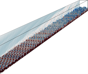
The configuration under investigation is a spatially evolving, zero-pressure-gradient flat-plate boundary layer, sketched in figure 1. The prescribed edge conditions of  $M_e=12.48$, $T_e=594.3\,\textrm {K}$ and $p_e=4656\,\textrm {Pa}$ are representative of those downstream of a shock wave generated by a $6^{\circ }$ sharp wedge flying at $M=20$ at an altitude of approximately 36 km. The stagnation enthalpy at the edge of the boundary layer is $H_e = h_e + u_e^2/2 = 18.66\,\textrm {MJ}\,\textrm {kg}^{-1}$, a value comparable to those of the high-enthalpy cases considered by Duan & Martín (Reference Duan and Martín2011b) and Di Renzo & Urzay (Reference Di Renzo and Urzay2021). Air at such free-stream conditions is supposed to be in thermochemical equilibrium ( $X_{\textrm {N}_2}=0.79$, $X_{\textrm {O}_2}=0.21$, $X_n$ being the $n$th species molar fraction). Of note, a similar scenario has been considered by Kline et al. (Reference Kline, Chang and Li2019) for stability studies. The computational domain is a rectangular box enclosed within the shock layer, highlighted in red in figure 1. The extent of the domain is $L_x \times L_y \times L_z = 3000 \delta ^{\star }_{in} \times 120 \delta ^{\star }_{in} \times 30 {\rm \pi}\delta ^{\star }_{in}$, with $x$,
$x$,  $y$ and $z$ denoting the streamwise, wall-normal and spanwise directions, respectively, and $\delta ^{\star }_{in}$ the displacement thickness of the boundary layer at the inlet section, computed as $\delta ^{\star }=\int _0^\delta (1-\rho u/\rho _e u_e)\,\textrm {d}y$ ( $\delta$ being the boundary-layer thickness at $99\,\%$ of the edge velocity). The computational grid is $N_x \times N_y \times N_z = 9660 \times 480 \times 512$, for a total of approximately 2.4 billions grid points. The grid spacing is uniform in the streamwise and spanwise directions, whereas a constant grid stretching of 0.7 % is applied in the wall-normal direction. The calculation is initiated in the laminar region at a distance $x_0$ from the plate leading edge. The profiles of the conservative variables prescribed at the inflow are generated by solving the locally self-similar theory for a two-dimensional chemically out-of-equilibrium and vibrationally equilibrated boundary layer (Sciacovelli et al. Reference Sciacovelli, Passiatore, Cinnella and Pascazio2021); the inflow Reynolds number based on the inlet displacement thickness is $Re_{\delta ^{\star }_{in}}=6054$. Using a thermal equilibrium simplifies the numerical setting and is not expected to alter the qualitative behaviour of the turbulent zone, of interest in the following analyses. A sponge layer is applied downstream of the inlet boundary, up to $(x-x_0)/\delta ^{\star }_{in} = 20$, to prevent abrupt distortions of the boundary layer. Characteristic-based boundary conditions are imposed at the top and right boundaries, and periodic conditions are set in the spanwise direction. The wall is assumed non-catalytic (i.e. $\partial Y_n/\partial y = 0$) and isothermal with $T=T_{V}=1800\,\textrm {K}$. The first condition implies that the surface does not participate to chemical processes. This is an idealization of what actually happens in practical flight conditions: the material of TPS of flight vehicles may be catalytic, thus promoting recombination of the atoms in the mixture in the near-wall region. The investigation of finite-rate catalysis is beyond the scope of the present discussion, but it could be of interest to understand the contribution of wall catalysis to thermal stresses (Bonelli, Pascazio & Colonna Reference Bonelli, Pascazio and Colonna2021) in future works. On the other hand, the hypothesis of wall thermal equilibrium is mainly dictated by a lack of knowledge about the most appropriate conditions to be used for vibrational temperature. In previous studies of laminar flows around hollow cylinder flares (Kianvashrad & Knight Reference Kianvashrad and Knight2017, Reference Kianvashrad and Knight2019), both adiabatic and isothermal boundary conditions where utilized for the vibrational energy, leading to similar results in terms of heat transfer. Furthermore, past boundary-layer stability studies accounting for thermal non-equilibrium assumed thermal equilibrium at the wall (Bitter & Shepherd Reference Bitter and Shepherd2015; Kline et al. Reference Kline, Chang and Li2019; Knisely & Zhong Reference Knisely and Zhong2019). Unfortunately, no information is available for turbulent flows. Nevertheless, the contribution of the vibrational heat transfer to the total wall heat flux will be shown to be small with respect to the roto-translational counterpart (as later detailed in § 3), justifying a posteriori the choice of a Dirichlet boundary condition as a first approximation. The selected wall temperature value, on the other hand, is representative of realistic flight data (Park Reference Park2004).

Figure 1. Sketch of the configuration under investigation.
Transition to turbulence is induced by means of a suction and blowing strategy, similar to the one adopted in Passiatore et al. (Reference Passiatore, Sciacovelli, Cinnella and Pascazio2021). Specifically, the following wall-normal velocity is imposed along a wall strip close to the inflow:
 \begin{align} \frac{v_{wall}}{u_\infty} &= {\rm e}^{{-}0.4 g(x)^2} A \left[ \sin\left(2 {\rm \pi}g(x) - \omega t \right) + \cos(\beta z) \vphantom{\left(2 {\rm \pi}g(x) - \omega t+\frac{\rm \pi}{4}\right)}\right. \nonumber\\ &\left.\quad +\, 0.05 \sin \left(2 {\rm \pi}g(x) - \omega t+\frac{\rm \pi}{4}\right) \cos(\beta z) \right] , \end{align}
where  $g(x)=(x-x_{forc})/(\delta ^{\star }_{in}\sqrt {2}\sigma )$, with $\sqrt {2} \sigma = 0.85 ({2 {\rm \pi}}/{\omega })$ and $x_{forc}$ is the centre of the Gaussian-like distribution which modulates the forcing function. The Reynolds number at the forcing location is $Re_{\delta ^{\star }_{forc}}=10^4$, corresponding to $x_{forc}=7.4\times 10^{-2}$ m. In (2.19), the non-dimensional pulsation $\omega = \tilde {\omega } \delta ^{\star }_{in}/ c_\infty$ ( $c_\infty$ being the free-stream speed of sound) corresponds to a dimensional frequency of $\tilde {f}=\tilde {\omega }/2 {\rm \pi}=75\,\textrm {kHz}$ and $\beta = 0.4/ \delta ^{\star }_{in}$ is the spanwise wavenumber. Lastly, $A$ is the forcing amplitude, which has been set equal to $5\,\%$. The presence of stationary modes at a strong amplitude in the suction-and-blowing injection strip mimics the effects of roughness spots and is used to speed up breakdown to turbulence within the prescribed computational domain.
2.4. Data collection and analysis
In the results presented below, flow statistics are computed by averaging in time and in the spanwise homogeneous direction, after that the initial transient is evacuated. First- and second-order moments of various flow quantities will be presented and discussed. For a given variable  $f$, we denote with $\bar {f} = f - f'$ the standard time and spanwise average, with $f'$ the corresponding fluctuation, whereas $\tilde {f}= f - f''$ denotes the density-weighted Favre averaging, with $f''$ the Favre fluctuation and $\tilde {f} = \overline {\rho f} / \bar {\rho }$. The sampling time interval is constant and corresponds exactly to 300 samples per each period of the forcing harmonic; specifically, ${\rm \Delta} t_{stats}^+= {\rm \Delta} t_{stats} ({u^2_\tau \overline {\rho }_w}/{\overline {\mu }_w})= 0.16$, with $u_\tau = \sqrt { \overline {\tau }_w / \overline {\rho }_w }$ the friction velocity based on the averaged wall shear stress $\overline {\tau }_w$ at the end of the computational domain. Data are collected for more than three turnover times, corresponding to $T_{stats} ({u^2_\tau }/{\overline {\mu }_w/\overline {\rho }_w}) \approx 6700$ for a total of ${\approx }40\,000$ temporal snapshots. In addition to flow statistics, instantaneous planes and specific meshlines are extracted with a frequency twenty and forty times higher with respect to the fundamental mode in the forcing function, for a total of 3200 and 6400 samples, respectively. The analysis will mainly focus on five selected streamwise stations; one located in the laminar region (for purpose of comparison), one in the transitional region and the last three in the turbulent portion of the domain. Table 1 reports the values of the Reynolds number based on the distance from the leading edge $Re_x= \rho _e u_e x / \mu _e$ at the selected stations and some boundary-layer properties. The Reynolds number based on the local momentum thickness $Re_\theta =\rho _e u_e \theta / \mu _e$ (with $\theta =\int _0^\delta \rho u/\rho _e u_e(1-\rho u/\rho _e u_e)\,\textrm {d}y$) reaches values close to $\approx 6000$ in the fully turbulent region, corresponding to $Re_\theta ^{inc}=Re_\theta \mu _e/\overline {\mu }_w$ of approximately 3000. The displacement-thickness-based Reynolds number $Re_{\delta ^{\star }}=\rho _e u_e {\delta ^{\star }} / \mu _e$ and the friction Reynolds number $Re_\tau = \overline{\rho}_w u_\tau \delta / \overline {\mu }_w$ reach values up to ${\approx }16 \times 10^4$ and ${\approx }1100$, respectively. Of note, the grid spacings ensure a DNS-like spatial resolution everywhere. Here, the notation ‘ $\bullet ^+$’ denotes normalization with respect to the viscous length scale $l_v = \overline {\mu }_w/(\overline {\rho }_w u_\tau )$. Unless otherwise specified, the wall-normal evolution of statistics is displayed in inner semi-local units $y^{\star }=\bar {\rho } u_\tau ^{\star }y/\bar {\mu }$, with $u_\tau ^{\star }=\sqrt {\overline {\tau }_w/\bar {\rho }}$.
Table 1. Boundary-layer properties at five selected downstream stations. In the table,  $Ma_\tau = u_\tau /\overline {c}_w$ is the friction Mach number, $B_q^{TR}=q_w^{TR}/(\overline {\rho }_w u_\tau \overline {h}_w)$ and $B_q^{V}=q_w^{V}/(\overline {\rho }_w u_\tau \overline {h}_w)$ are the roto-translational and vibrational dimensionless heat fluxes. Lastly, ${\rm \Delta} x^+$, ${\rm \Delta} y^+_{w}$, ${\rm \Delta} y^+_\delta$ and ${\rm \Delta} z^+$ denote the grid sizes in inner variables in the $x$-direction, $y$-direction at the wall and at the boundary-layer edge and in the $z$-direction, respectively.

3. Results
3.1. Global flow properties
The streamwise evolution of selected quantities at the wall is first discussed. Figures 2(a) and 2(b) report the distributions of the skin friction coefficient  $C_f$ and the heat flux coefficients $C_{q}$ and $C_q^{V}$, defined as
 \begin{equation} C_f=\frac{2\overline{\tau}_w}{\rho_e u_e^2},\quad C_q^{TR} =\frac{\overline{q}_w^{TR}}{\rho_e u_e^3},\quad C_q^{V} =\frac{\overline{q}_w^{V}}{\rho_e u_e^3}, \end{equation}
the net total heat flux being given by the sum of the two contributions. A ramp up starting at  $(x-x_0)/\delta ^{\star }_{in} \approx 1100$ leads to a sharp overshoot in the $C_f$ profile, with a peak of the wall shear stress almost five times larger than its corresponding laminar value. The flow achieves a turbulent regime starting from $(x-x_0)/\delta ^{\star }_{in} \approx 1800$, with a smoothly decreasing $C_f$ up to the end of the computational domain. The roto-translational contribution of the wall heat flux $C_q^{TR}$ is shown to be largely predominant with respect to the vibrational counterpart $C_q^{V}$ (which is multiplied by ten to match the range of figure 2b), mainly because of the vibrational thermal conductivity $\overline {\lambda _{V}}$, whose values are approximately one order of magnitude smaller than $\overline {\lambda _{TR}}$. While $C_q^{TR}$ closely follows the skin friction coefficient profile, $C_q^{V}$ exhibits a different evolution. It rapidly decreases after the forcing strip and stays approximately constant up to the breakdown to turbulence; afterwards, the value in the turbulent region almost doubles the one in the laminar regime and keeps a constant value up to the end of the domain. The different trend of the heat fluxes is related to the evolution of vibrational temperature gradients across the boundary layer, as discussed later in § 3.3. In order to isolate the contributions of the mean and fluctuating field to the skin friction, the decomposition of Renard & Deck (Reference Renard and Deck2016) (later extended to compressible flows by Li et al. Reference Li, Fan, Modesti and Cheng2019) has been computed; of note, the general hypotheses under which it is derived allows a straightforward application even in presence of thermal and chemical non-equilibrium effects. The skin friction coefficient can then be rewritten under the following form:
 \begin{align} C_f &= \underbrace{\frac{2}{\rho_\infty u^3_\infty} \int_0^\delta \overline{\tau}_{xy} \frac{\partial \tilde{u}}{\partial y} \text{d}y}_{C_{f,1}}+ \underbrace{\frac{2}{\rho_\infty u^3_\infty} \int_0^\delta -\overline{\rho u''v''} \frac{\partial \tilde{u}}{\partial y} \text{d}y}_{C_{f,2}} \nonumber\\ &\quad + \underbrace{\frac{2}{\rho_\infty u^3_\infty} \int_0^\delta ( \tilde{u} - u_\infty) \left[ \bar{\rho} \left( \tilde{u}\frac{\partial \tilde{u} }{\partial x} +\tilde{v} \frac{\partial \tilde{u}}{\partial y} \right) - \frac{\partial}{\partial x} \left( \overline{\tau}_{xx} - \bar{\rho} \widetilde{u''u''} -\bar{p} \right) \right] \text{d}y } _{C_{f,3}} , \end{align}
where  $C_{f,1}$, $C_{f,2}$ and $C_{f,3}$ represent the mean-field molecular dissipation, the turbulent dissipation and the effects related to boundary-layer spatial growth, respectively. The sum of the three terms and their separate contributions are displayed in figure 3. An excellent agreement with respect to the direct $C_f$ computation is observed in the pseudo-laminar and fully turbulent regions, with only minor deviations in the transition region. The $C_{f,3}$ contribution is negligible everywhere but at the breakdown-to-turbulence location, where it takes negative values due to the abrupt thickening of the boundary layer. The decrease of $C_{f,3}$ is counterbalanced by a large increase of the Reynolds stress-related term, whereas the growth of the mean-field contribution, $C_{f,1}$, is slightly delayed with respect to the other two. In the turbulent region, $C_{f,1}$ and $C_{f,2}$ are almost superposed, differently from what observed by Passiatore et al. (Reference Passiatore, Sciacovelli, Cinnella and Pascazio2021) where the former was shown to be predominant. Such a discrepancy can be ascribed to the much larger friction Reynolds numbers reached in the current configuration, leading to an increased turbulent contribution (Fan, Li & Pirozzoli Reference Fan, Li and Pirozzoli2019).

Figure 2. Evolution of (a) the skin friction coefficient  $C_f$ (black line) and (b) the heat flux coefficients $C_q^{TR}$ and $C_q^{V}$ (black and red lines, respectively). The filled symbols in (a) denote the streamwise location of the five stations selected in table 1.

Figure 3. Evolution of (a) the skin friction coefficient  $C_f$ (black line) and Renard–Deck decomposition (red symbols) and (b) separate contribution of each term of (3.2).
3.2. Mean flow analysis
Different scalings for the profiles of the averaged streamwise velocity have been tested. First, the transformations of Van Driest (Reference Van Driest1956) and Trettel & Larsson (Reference Trettel and Larsson2016)
 \begin{equation} u_{VD} = \frac{1}{u_\tau} \int_0^{\bar{u}} {\sqrt{\frac{\bar{\rho}}{\overline{\rho}_w}}}\,\text{d}u,\quad u_{TL} = \int_0^{ \bar{u}}{\left(\frac{\bar{\rho}}{\overline{\rho}_w}\right) \left[ 1 + \frac{1}{2} \frac{1}{\bar{\rho}} \frac{\text{d}\bar{\rho}}{\text{d}y} y - \frac{1}{\bar{\mu}} \frac{\text{d}\bar{\mu}}{\text{d}y} y \right] } \text{d}u \end{equation}
are shown for the three turbulent stations in figures 4(a) and 4(b), respectively. The former scaling has been shown to work reasonably well for adiabatic boundary layers, even at high speeds (Passiatore et al. Reference Passiatore, Sciacovelli, Cinnella and Pascazio2021). On the other hand, it becomes inaccurate when highly cooled configurations are considered, whether they be boundary layers (Zhang et al. Reference Zhang, Duan and Choudhari2018; Huang et al. Reference Huang, Nicholson, Duan, Choudhari and Bowersox2020), pipe flows (Ghosh, Foysi & Friedrich Reference Ghosh, Foysi and Friedrich2010) or channel flows (Modesti & Pirozzoli Reference Modesti and Pirozzoli2016; Sciacovelli, Cinnella & Gloerfelt Reference Sciacovelli, Cinnella and Gloerfelt2017). Figure 4(a) confirms such a trend, both the linear and logarithmic regions being offset with respect to the analytical laws. Of note, in figure 4 the logarithmic region is described by  $(1/\kappa )\log y^+ + C$ and $(1/\kappa )\log y^* + C$, with $\kappa =0.41$ and $C=5.2$. The semi-local scaling of Trettel & Larsson, as expected, improves the near-wall prediction since it explicitly accounts for the stress-balance condition within the entire inner layer. A large scatter is, however, observed in the logarithmic region which shows a $Re$-dependence similar to the van Driest scaling. Although such a scaling works reasonably well for internal flows, it is not as good for external configurations, most likely because of an interaction with the wake region which is shown to be over-stretched in figure 4(b). Recently, Griffin, Fu & Moin (Reference Griffin, Fu and Moin2021) proposed a new total-stress-based transformation (called hereafter Griffin–Fu–Moin scaling, $u_{GFM}$) with a constant-stress-layer assumption, which reads
 \begin{equation} u_{GFM} = \int_0^{\delta}\frac{\dfrac{1}{\mu^+} \dfrac{\partial u^+}{\partial y^*}}{1+\dfrac{1}{\mu^+} \dfrac{\partial u^+}{\partial y^*} - \mu^+ \dfrac{\partial u^+}{\partial y^+}} \text{d}y^* \end{equation}
where  $\mu ^+$ denotes normalization of the mean viscosity with respect to its wall value. Such a scaling has been shown to successfully collapse channels, pipe flows and boundary-layer configurations, even at large Mach numbers. A comparison between $u_{TL}$ and $u_{GFM}$ as a function of $y^\star$ is shown in figure 4(c) for a velocity profile extracted at $Re_\theta =6200$. In the inner layer, viscous stresses are predominant and roughly correspond to the total shear stress resulting in a very good collapse for both scalings. On the contrary, turbulent shear stresses become dominant in the logarithmic region, which effect is most correctly taken into account by the total-stress-based scaling. This results in a better collapse of $u_{GFM}$ onto the universal logarithmic profile with respect to $u_{TL}$, for which the slope of the logarithmic region is largely overestimated. Yet, the $u_{GFM}$ transformation still predicts a higher slope and intercept in the logarithmic region compared with the classical incompressible values, in accordance with the recent study of Lee, Martin & Williams (Reference Lee, Martin and Williams2021). Finally, we verified that the transformation based on the constant-stress-layer assumption (i.e. $\tau /\tau _w \approx 1$ across the boundary layer, leading to (3.4)) and the one based on the actual total shear stress (extracted from DNS data) do not exhibit any discernible differences, confirming the validity of the constant-stress-layer hypothesis. Neither chemical activity nor thermal relaxation process should substantially alter the validity of the transformation since a certain degree of decoupling is observed between the thermochemical and turbulent activities, as previously noticed by Passiatore et al. (Reference Passiatore, Sciacovelli, Cinnella and Pascazio2021) and Di Renzo & Urzay (Reference Di Renzo and Urzay2021).

Figure 4. Wall-normal profiles of (a) the van Driest-transformed streamwise velocity, (b) Trettel & Larsson's transformation and (c) comparison between Trettel & Larsson transformation and total-stress-based scaling of Griffin et al. (Reference Griffin, Fu and Moin2021) at  $Re_\theta = 6200$.
Figure 5 shows the Reynolds stress profiles at the turbulent station  $Re_\theta =6200$ normalized with respect to the semi-local friction velocity $u_\tau ^\star$; results are compared with low-enthalpy configurations extracted from Zhang et al. (Reference Zhang, Duan and Choudhari2018) (cases M14Tw018 and M8Tw048) and Xu et al. (Reference Xu, Wang, Wan, Yu, Li and Chen2021) (case M8T1). Despite the important differences in the values of the free-stream Mach numbers, friction Reynolds numbers, absolute wall temperatures and wall-cooling rates, the turbulent intensity profiles are comparable and do not exhibit any marked influence attributable to TCNE effects. Consistently with previous observations (Duan et al. Reference Duan, Beekman and Martín2011; Lagha et al. Reference Lagha, Kim, Eldredge and Zhong2011; Zhang et al. Reference Zhang, Duan and Choudhari2018), the larger streamwise component and the smaller cross-flow one may indicate the presence of strong compressibility effects, as discussed later in § 3.6. Another scaling often investigated in wall-bounded compressible turbulence is the one that relates the mean velocity to the mean temperature profile for zero-pressure-gradient boundary layers. The modified Crocco relation derived by Walz (Reference Walz1969) writes
 \begin{equation} \frac{\tilde{T}}{T_e} = \frac{T_w}{T_e}+ \frac{T_{aw}-T_w}{T_e} \left( \frac{\tilde{u}}{u_e} \right) + \frac{T_e-T_{aw}}{T_e} \left( \frac{\tilde{u}}{u_e} \right)^2, \end{equation}
with  $T_{aw}/T_e= 1+r({(\gamma -1)}/{2})M_e^2$ and $r$ the recovery factor set equal to 0.9; the relation is shown in figure 6(a). In previous studies with high Mach numbers, wall-cooled, high-enthalpy boundary layers (Duan & Martín Reference Duan and Martín2011b), it was found that such a relation deviates from the exact $\tilde {T}/T_e$ profile extracted from DNS data; a significant discrepancy is indeed shown in the range $0.2 < \tilde {u}/u_e <0.7$. This should not be surprising since relation (3.5) was derived under calorically perfect gas hypotheses. In order to remove the explicit dependence on thermal and chemical models, Duan & Martín (Reference Duan and Martín2011b) proposed an analogous enthalpy-based equation, which reads
 \begin{equation} \frac{\tilde{h}}{h_e} = \frac{h_w}{h_e}+ \frac{h_{aw}-h_w}{h_e} f\left( \frac{\tilde{u}}{u_e} \right) - r \frac{u_e^2}{2 h_e}\left(\frac{\tilde{u}}{u_e} \right)^2, \end{equation}
where  $h_{aw}= h_e + \frac {1}{2}ru_e^2$. The function $f(\tilde {u}/u_e)$ has to be independent of free-stream conditions, wall temperature and surface catalysis (if any). For calorically perfect gases, (3.6) reduces to (3.5), apart from the term $f(\tilde {u}/u_e)$ which is equal to $\tilde {u}/u_e$ in the classical formulation. By curve fitting the DNS data, Duan & Martín (Reference Duan and Martín2011b) obtained the following relation for $f(\tilde {u}/u_e)$:
 \begin{equation} f \left( \frac{\tilde{u}}{u_e} \right) =0.1741\left( \frac{\tilde{u}}{u_e} \right) ^2 + 0.8259 \left(\frac{\tilde{u}}{u_e} \right). \end{equation}
The results of this transformation are displayed in figure 6(b) and show an improved collapse with respect to the classical temperature-based formulation.

Figure 5. Reynolds stresses in the (a) streamwise, (b) wall-normal and (c) spanwise directions, and (d) Reynolds shear stress. The M14Tw018 and M8Tw048 profiles are extracted from Zhang et al. (Reference Zhang, Duan and Choudhari2018), whereas M8T1 is from Xu et al. (Reference Xu, Wang, Wan, Yu, Li and Chen2021).


3.3. Thermal non-equilibrium effects
The presence of thermal non-equilibrium is analysed by comparing the vibrational relaxation time with characteristic time scales of the dynamic field. For that purpose, the following vibrational Damköhler numbers are considered:
 \begin{equation} {Da}_v^{VS} = \frac{\overline{\mu}_w/\overline{\tau}_w}{t_m},\quad {Da}_v^{LE} = \frac{\delta^{{\star}}/u_\tau}{t_m},\quad {Da}_v^{RT} = \frac{x/u_e}{t_m}, \end{equation}
with  ${Da}_v^{(\bullet )} = \mathcal {O}(1)$ denoting the regime in which non-equilibrium effects are relevant. The numerator of each Damköhler number is fixed for a given streamwise station and equal for each of the three molecules; the different trends of these parameters, for each of the three diatomic species, are therefore entirely dictated by the species molecular relaxation times $t_m$, which depend upon the local state of the gas. The evolution of these dimensionless numbers is displayed in figure 7. The first ratio in (3.8a–c) relates the characteristic time of fluid motion in the viscous sublayer (VS) to the vibrational relaxation time of molecule $m$. Figure 7(a,d,g) shows the evolution of this quantity for the three molecules present in the mixture. It is shown that ${Da}_v^{VS} \ll 1$ everywhere for N $_2$ and O $_2$ whereas it is of the order of unity only for NO, whose concentration is, however, almost negligible (see § 3.5). The decoupling of the two time scales indicates that there exists a layer of thickness $l_v$ in the inner (colder) region of the boundary layer in which the molecules are vibrationally frozen. The higher values of ${Da}_v^{VS} \ll 1$ observed at the laminar position are due to the predominance of viscous stresses. Of major interest is ${Da}_v^{LE}$, representing the ratio between the large-eddy (LE) turnover time and the relaxation time, constructed by means of the displacement thickness $\delta ^{\star }$ and $u_\tau$. The orders of magnitude of the two time scales are comparable for molecular nitrogen (figure 7b), for which the peak of ${Da}_v^{{LE}}$ ranges from 0.4 to 0.7 at $y^{\star } \approx 10$ as the flow evolves in the turbulent region. On the other hand, figures 7(e) and 7(h) show that ${Da}_v^{{LE}}\gg 1$ for O $_2$ and NO, implying that the two molecules reach a vibrational equilibrium with respect to the characteristic time of the large-scale turbulent motions much faster. Similar considerations hold for ${Da}_v^{RT}$, which compares the vibrational relaxation time with the local flow residence time (RT). As the flow evolves along the plate, there is enough time for O $_2$ and NO to achieve thermal equilibrium, whereas N $_2$ remains significantly out of equilibrium at all stations. This result is a consequence of the high vibrational temperature (and slower relaxation rate) characteristic of molecular nitrogen. Of note, both ${Da}_v^{LE}$ and ${Da}_v^{RT}$ exhibit much higher values at the three turbulent stations due to the contribution of turbulent mixing. Wall-normal profiles of the normalized mean translational and vibrational temperatures are reported in figures 8(a) and 8(b), respectively. The translational temperature reaches a peak value of approximately $[2.3-2.5]T_w$, at a wall-normal location $y^{\star }\approx 10$, corresponding to the peak of turbulent intensity. The vibrational temperature $\widetilde {T_{V}}$ is 20 % to 30 % smaller than $\tilde {T}$ across the boundary layer, proving the existence of a vibrational–relaxation layer for the thermodynamic conditions under investigation, and also exhibits a peak located between the buffer layer and the lower logarithmic region. The major gap is visible at $Re_\theta =2960$, which corresponds to the $C_f$ peak. Additionally, the wall gradient $\partial \widetilde {T_{V}}/\partial y^{\star }$ is little sensitive to the peak's magnitude and location, explaining the nearly constant trend of $C_q^{V}$ previously observed in figure 2(b).

Figure 7. Vibrational Damköhler numbers for N $_2$ (a–c), O $_2$ (d–f) and NO (g–i). Damköhler number based on inner units (a)-(d)-(g), large-eddy turnover times (b)-(e)-(h) and flow residence time (c)-(f)-(i).

Figure 8. Normalized mean translational temperature (a) and vibrational temperature (b) at the selected streamwise stations.
The normalized temperature difference  $(\tilde {T}-\widetilde {T_{V}})/T_w$ is reported in figure 9(a,b) as a function of $y^\star$ and $y/\delta$, respectively. Such a quantity increases in the transitional region, reaches a maximum of the order of ${\approx }2000\,\textrm {K}$ where $C_f$ peaks, and then tends to decrease moving towards the turbulent region. The wall-normal maximum value moves from the outer part of the boundary layer ( $y/\delta \approx 0.6$) to the buffer layer, where it stabilizes at $y^\star \approx 8$. Thermodynamic non-equilibrium conditions are kept until the end of the computational domain, as already confirmed by inspection of the vibrational Damköhler number values. Positive $\tilde {T}-\widetilde {T_{V}}$ values are observed from the VS (we recall that $T = T_{V} = 1800\,\textrm {K}$ at the wall) up to the first portion of the logarithmic region. However, as the flow evolves along the flat plate, a region characterized by $\tilde {T}-\widetilde {T_{V}}<0$ appears, meaning that the flow becomes vibrationally over-excited. The height at which the sign changes smoothly moves from the edge of the boundary layer up to $y/\delta \approx 0.45$, due to the boundary-layer thickening. This is clearly visible in figure 10, where we report a snapshot of the temperature difference along a longitudinal cut plane (top) and the isocontours of the second invariant of the velocity gradient tensor coloured by $(T-T_{V})$. Fiévet et al. (Reference Fiévet, Voelkel, Raman and Varghese2019), who conducted an analysis on the coupling between vibrational non-equilibrium and turbulent mixing, observed that the majority of non-equilibrium states occur in under-excited conditions. The rare regions in which there exists an over-excited non-equilibrium state are dictated by the link between the roto-translational and mechanical energies. The static temperature is coupled with the other variables through the equation of state; hence, a decrease of turbulent intensity (moving towards the edge of the boundary layer) produces a decrease of the translational temperature. At the same time, the vibrational energy remains nearly constant because it relaxes slowly, leading to an over-excitation in the outer layer, until the free-stream equilibrium conditions are reached by both temperatures.

Figure 9. Normalized difference  $(\tilde {T}-\widetilde {T_{V}})/T_w$ at the selected streamwise stations; (a) semi-local units, (b) outer scale. The dotted line corresponds to the zero value.

Figure 10. Instantaneous isocontours of  $T-T_{V}$ in a $xy$-plane and second invariant of the velocity gradient tensor, $Q$, coloured by $T-T_{V}$.
Normalized root mean square (r.m.s.) of the Favre fluctuations of translational and vibrational temperatures across the boundary layer are displayed in figure 11. In figure 11(a), a peak emerges on each side of the  $\tilde {T}_{max}$ location ( $y^{\star }\approx 10$), as classically observed for wall-cooled TBLs (Duan, Beekman & Martín Reference Duan, Beekman and Martín2010; Zhang et al. Reference Zhang, Duan and Choudhari2018; Di Renzo & Urzay Reference Di Renzo and Urzay2021). The predominance of the outer r.m.s. peak in the turbulent region is mainly caused by the decrease of $\tilde {T}$ toward the outer boundary, the absolute temperature fluctuations being comparable in the inner and outer regions. In contrast, the vibrational temperature fluctuations exhibit no local minimum (figure 11b), and increase monotonically up to the boundary-layer edge, where they drop abruptly. This is in contrast to profiles typically observed in the laminar region (see the profile at $Re_\theta =1600$ reported in the figure for comparison), and can be ascribed to thermal non-equilibrium: the vibrational relaxation times being slower than the translational ones and comparable to the turbulence time scales, $T_{V}$ variations due to vibrational–translational energy exchanges occur at similar rates than variations caused by wall-normal turbulent motions. Therefore, the latter play a major role in redistributing vibrational temperature across the boundary layer, smoothing out the local minimum. The premultiplied energy spectra of the fluctuating temperatures, reported in figure 12 as a function of the normalized spanwise wavenumber $\lambda ^{\star }$, provide a further confirmation of this trend. For both temperatures, a large-scale peak is visible at $\lambda _z^{\star } \approx 1500$ and $y^{\star } \approx 2500$, whereas an inner (slightly weaker) peak is observed only for the roto-translational temperature spectrum, coherently with the r.m.s. temperature fluctuations. Additionally, the well-developed spectra indicate that a fully turbulent state has been reached and the footprint of the forcing strategy has been completely lost. The persistence of thermal non-equilibrium conditions across the boundary layer is tightly related to the transition to a turbulent regime. Preliminary numerical experiments on the same configuration without boundary-layer tripping have shown that, for a laminar flow regime, the difference between the roto-translational and vibrational temperatures is almost negligible (of the order of 50 K) at the end of the plate. The thermal non-equilibrium observed in the turbulent case is strongly related to sweep and ejection turbulent motions, resulting in enhanced mixing as anticipated by Urzay & Di Renzo (Reference Urzay and Di Renzo2021) with a priori considerations. In figure 13 we report the mean values of the two temperatures conditioned on sweep events (characterized by $u''>0$ and $v''<0$) and ejection events ( $u''<0$ and $v''>0$) at $Re_\theta = 6200$ and for several wall-normal locations. Within the VS, sweeps entrain hot fluid from the overlying regions. Consequently, they are characterized by higher mean temperatures with respect to the total average in the inner region. The opposite is true for ejection events. The largest differences between sweeps and ejections conditionally averaged temperatures are registered for the roto-translational modes due to the sharper peak observed for $\tilde {T}$. An opposite trend is observed at normal locations beyond the temperature peak ( $y^\star \approx 10$). In this case, sweeps bring colder air from the outer layers towards the hotter, inner region; here, the translational modes rapidly reach equilibrium, whereas a longer relaxation time is needed for the vibrational ones. As a result, $\widetilde {T_{V}}$ is always smaller than $\tilde {T}$. On the other hand, ejection motions bring hotter, thermally out-of-equilibrium mixture towards the outer region of the boundary layer, where vibrational relaxation times rapidly increase because of the colder environment; therefore, in this region $\widetilde {T_{V}}>\tilde {T}$. The largest temperature difference between sweeps and ejections events occurs in the first portion of the logarithmic region (up to $y^\star \approx 100$), with values as large as 800 K for vibrational modes and 1000 K for the roto-translational ones. Further evidence of this phenomenon is provided by the conditional probability density functions (p.d.f.s) of the two temperatures, shown in figure 14. Three wall-normal stations are considered: the location where the maximum temperature difference is registered (panels a and b, $y^{\star } \approx 10$), the logarithmic region (panels c and d, $y^{\star } \approx 100$) and the boundary layer edge (panels e and f, $y^{\star } \approx 3000$). Close to the boundary layer edge, a heavy right tail is observed for the p.d.f.s of both events, with $T_{V}$ values slightly larger than $T$ ones. Moving inside the boundary layer, at $y^\star \approx 100$, both p.d.f.s tend to become symmetric. The most remarkable differences are observed in the buffer layer with left-skewed distributions for $T$ and symmetric ones for $T_{V}$, their shape being related to the presence of a local minimum for $\widetilde {T''^2}$ and a small plateau for $\widetilde {T_{V}''^2}$ as shown in figure 11.

Figure 11. Root-mean-square temperature Favre fluctuations normalized by the local Favre average for translational temperature (a) and vibrational temperature (b).

Figure 12. Premultiplied energy spectra  $k_z E_{T' T'}/\bar {T}$ (a) and $k_z E_{T'_{V} T'_{V}}/\overline {T_{V}}$ (b), at $Re_\theta =6200$.

Figure 13. Mean values of  $\tilde {T}$ and $\widetilde {T_{V}}$ conditioned on sweep and ejection events, at $Re_\theta = 6200$ at various wall-normal heights. Blue lines: roto-translational modes; red lines: vibrational modes; dashed lines, diamonds: average over sweep events; dashed-dotted lines, triangles: average over ejection events; solid lines, circles: global average.

Figure 14. Conditional probability density function (p.d.f.) of translational and vibrational temperatures at  $Re_\theta =6200$ for $y^{\star }$ approximately equal to 10, 100 and 3000, respectively; sweeps events (a,c,e) and ejections events (b,d,f).
3.4. Thermal modelling and Reynolds analogies
For thermally out-of-equilibrium flows, a new unclosed term appears by Favre averaging the vibrational energy equation (2.5), namely, the turbulent transport of vibrational energy  $\overline {\rho u''_j e''_V}$. Such a term is the analogue of the turbulent transport term appearing in the total energy equation. The latter is usually modelled by introducing a turbulent Prandtl number $Pr_{t}$, defined as
 \begin{equation} Pr_t=\frac{\overline{\rho u''v''} \partial \tilde{T}/\partial y}{\overline{\rho v''T''} \partial \tilde{u}/\partial y}. \end{equation}
According to the classical strong Reynolds analogy (SRA),  $Pr_t$ is expected to take values close to one throughout the flow (Morkovin Reference Morkovin1962). Figure 15(a) (displayed in external units for better clarity) shows that the estimation fails at the peak of $\tilde {T}$, located at $y/\delta \approx 0.03$, since the coexistence of null temperature gradient and turbulent heat flux causes an overshoot. Such a behaviour was previously observed by Duan & Martín (Reference Duan and Martín2011b) and Di Renzo & Urzay (Reference Di Renzo and Urzay2021) (for a discussion about the validity of this assumption for adiabatic hypersonic boundary layers, see Passiatore et al. Reference Passiatore, Sciacovelli, Cinnella and Pascazio2021). By analogy, the turbulent flux of vibrational energy can be modelled by introducing a vibrational turbulent Prandtl number
 \begin{equation} Pr_t^{V}=\frac{\overline{\rho u''v''} \partial \widetilde{T_{V}}/\partial y}{\overline{\rho v''T_{V}''} \partial \tilde{u}/\partial y}. \end{equation}
Here,  $Pr_t^{V}$ (shown in figure 15b) takes values close to unity in a relatively large region corresponding to $0.2 \lessapprox y/\delta \lessapprox 0.7$, where turbulent transport dominates, and it diverges at the boundary-layer edge (where $\partial \tilde {u}/\partial {y}$ tends to vanish) and close to the wall, similarly to $Pr_t$. We can get further insights by reporting, in figure 16, correlations of $u''$ and $v''$ fluctuations with $T''$ and $T_{V}''$, respectively. As observed in both low- and high-enthalpy boundary layers (Zhang et al. Reference Zhang, Duan and Choudhari2018; Di Renzo & Urzay Reference Di Renzo and Urzay2021), the logarithmic and outer regions are characterized by a negative correlation between $u''$ and $T''$ (a) and positive correlation for $v''$ and $T''$ (b). This comes from (i) sweeps ( $u''>0$, $v''<0$) entraining colder ( $T''<0$) fluid towards the buffer layer, and (ii) ejections ( $u''<0$, $v''>0$) entraining hotter ( $T''>0$) fluid towards the edge, resulting in $R_{u''T''}<0$ and $R_{v''T''}>0$. Below the buffer layer, both correlations change their sign for the same reason, consistently with the trend previously discussed in figure 13. Similar considerations hold for $R_{u''T_{V}''}$ and $R_{v''T_{V}''}$. However, while streamwise velocity fluctuations close to the wall are perfectly correlated with the translational temperature ones ( $R_{u''T''} \approx 1$), the correlation coefficient with the vibrational temperature (c) is weaker ( $R_{u''T_{V}''}$ is between 0.7 and 0.85). This effect is attributed once again to the larger relaxation time of vibrational modes, $T_{V}$ needing more time than $T$ for adapting to the surrounding temperature. Together with the evolution of $Pr_t$ and the temperature–velocity fluctuation correlations, the SRA hypothesis also predicts that
 \begin{equation} \frac{T''/\tilde{T}_{rms}}{(\gamma -1) M^2 (u''/\tilde{u}_{rms})} \approx 1. \end{equation}
As already observed in the literature, the relation in (3.11) exhibits large deviations from the SRA estimation (not shown) since it fails to take into account the diabatic behaviour of the wall. Several modified forms have been proposed, one of the most successful being that of Huang, Coleman & Bradshaw (Reference Huang, Coleman and Bradshaw1995)
 \begin{equation} \frac{T''/\tilde{T}_{rms}}{(\gamma -1) M^2 (u''/\tilde{u}_{rms})} \approx \frac{1}{Pr_t(1 - (\partial \widetilde{T_t}/\partial \tilde{T}))}, \end{equation}
usually referred to as HSRA, with  $T_t$ the stagnation temperature. By removing the assumption of calorically perfect gas (Duan & Martín Reference Duan and Martín2011b), one can write a generalized HSRA (GHSRA)
 \begin{equation} T''_{rms} \approx{-}\frac{1}{Pr_t} \frac{\partial \tilde{T}}{\partial \tilde{u}}u''_{rms}. \end{equation}
The wall-normal evolution of the ratio between the right- and the left-hand sides of (3.13) is plotted in figure 17(a), where a satisfactory agreement is observed for most of the boundary-layer thickness (at least in regions where both velocity and temperature fluctuations are not nullified). By using the same procedure followed for  $Pr_t$, the GHSRA can also be extended to the vibrational temperature such that
 \begin{equation} T''_{{V,rms}} \approx{-}\frac{1}{Pr_t^{V}} \frac{\partial \widetilde{T_V}}{\partial \tilde{u}}u''_{rms}. \end{equation}
The results shown in figure 17(b) prove that the GHSRA maintains its validity under thermal non-equilibrium conditions and holds also for vibrational energy.
In addition to turbulent transport, further attention should be paid to the modelling of the nonlinear turbulence–thermal non-equilibrium interactions induced by the source terms of the vibrational energy equation, which are associated with translational–vibrational energy exchanges ( $Q_{TV}$) and chemical dissociation/recombination processes ( $\sum _m \dot {\omega }_me_{Vm}$). While thermal non-equilibrium can be reasonably quantified by the magnitude of $\tilde {T}-\widetilde {T_V}$, the analysis of the source terms allows one to isolate the physical processes originating such non-equilibrium conditions in the first place. In this specific configuration, chemical activity is extremely weak and therefore $\sum _m \dot {\omega }_me_{Vm}$ is almost negligible; as a consequence, changes in $\tilde {T}-\widetilde {T_V}$ are tightly related to $\overline {Q_{TV}}$ values. Positive values indicate vibrational under-excitation since $T>T_{V}$ (and the opposite for negative values). The wall-normal profiles of $\overline {Q_{TV}}$, shown in figure 18(a) as a function of $y^\star$ and $y/\delta$, closely follow those shown for $(\tilde {T} - \widetilde {T_{V}})$ in figures 9(a) and 9(b), albeit that the negative values visible in the zoomed view of the outer region are much less pronounced (two orders of magnitude lower) than those registered in the inner zone. Such a large difference is due to the concurrent effects of lower absolute temperature values and (to a lesser extent) smaller $(\tilde {T} - \widetilde {T_{V}})$ differences, causing the denominator to increase and the numerator to decrease in (2.15), respectively. Although the physical significance of $(\tilde {T} - \widetilde {T_{V}})$ and $\overline {Q_\textrm {TV}}$ is similar in the present case, the interest in analysing the latter quantity stems from a modelling standpoint; that is, only an appropriate modelling of the source term can ensure a correct description of the non-equilibrium state. In this respect, following the technique used by Duan & Martín (Reference Duan and Martín2011a) for assessing turbulence/chemistry interactions and with the aim of quantifying the coupling between turbulence and thermal relaxation, we built an indicator defined as
 \begin{equation} Q_{TV}^I = \frac{\overline{Q_{TV}(T,T_{V},\rho,p,Y_n)} - Q_{TV}(\tilde{T},\widetilde{T_{V}}, \bar{\rho}, \bar{p}, \widetilde{Y_n})}{\overline{Q_{TV}}_{,max}}, \end{equation}
where  $\overline {Q_{TV}}_{,max}$ denotes the maximum wall-normal value of $\overline {Q_{TV}}$ at the selected station. Deviations from null values represent a measure of vibrational energy variations associated with turbulent fluctuations. Figure 18(b) shows that computing $Q_{TV}$ from averaged quantities would underestimate its value across the whole boundary layer, with discrepancies larger than 15 % of $\overline {Q_{TV}}_{,max}$ in the inner layer. These data further confirm the tight coupling between thermal non-equilibrium and turbulence discussed in the current section and underline that attention must be paid to the development of suitable turbulence closures, especially in the context of RANS modelling.

Figure 15. Turbulent Prandtl number (a) and turbulent vibrational Prandtl number (b).

Figure 16. Correlation coefficients between Favre fluctuations of vibrational temperature and streamwise velocity (a) and wall-normal velocity (b) and of translational temperature and streamwise velocity (c) and wall-normal velocity (d).


Figure 18. Wall-normal profiles of (a)  $\overline {Q_{TV}}\ [J/(m^{3}\ s)]$ and (b) $Q_{TV}^I$, defined in (3.15). In the inset of (a), a zoom of the profile is shown in outer scale; the dashed line denotes the null value.
3.5. Chemical activity
In this section we investigate chemical activity triggered in the high-enthalpy boundary layer by friction heating. The profiles of Favre-averaged mass fractions of species present in the mixture are reported in figure 19. At the flow conditions under investigation, molecular oxygen is the species which dissociates most, leading to the formation of atomic oxygen. The maximum mass fraction of atomic oxygen in the mixture is approximately  $1\,\%$. The maximum temperatures in the boundary layer are too low to allow nitrogen dissociation in any significant amount, even at the temperature peak, and consequently the quantity of atomic nitrogen is negligible compared with the other species. Nevertheless, the present conditions are such that a small amount of nitric oxide (approximately $0.7\,\%$) is produced by the forward shuffle reaction R4 and by the backward shuffle reaction R5. The rather low chemical activity is partly due to the strong wall cooling, limiting the maximum temperature to values just above the threshold for oxygen dissociation ( $T>2000\,\textrm {K}$). Thermal non-equilibrium further limits chemical reactions. Highly vibrationally excited molecules are meant to dissociate more rapidly, since they require less energy exchange during the collisions. On the contrary, in under-excitation conditions, dissociation is less likely to occur. This mechanism is numerically taken into account in the computation of the reaction rate coefficients (for the calculation of which a geometric average of the two temperatures is considered, $T^{0.7}T_{V}^{0.3}$); they turn out to be lower when strong non-equilibrium effects are present. On the other hand, the endothermic chemical reactions tend to drain roto-translational energy, although this effect is partly compensated by the relaxation of vibrational modes, which supply energy and partly counteract temperature reduction. The chemical Damköhler number based on the LE turnover time $(\delta ^{\star }/u_\tau )/(\overline {\rho /\dot {\omega }_n})$ is at most of the order of $10^{-2}$ for all species, denoting little interaction between chemical reactions and turbulent motions and an almost frozen-chemistry behaviour. A detailed discussion can be found in Passiatore et al. (Reference Passiatore, Sciacovelli, Cinnella and Pascazio2021) for an adiabatic turbulent chemically out-of-equilibrium boundary layer; despite the different conditions, similar qualitative observations can be made in the present work.

Figure 19. Mean mass fraction of molecular nitrogen (a), molecular oxygen (b), nitric oxide (c), atomic oxygen (d) and atomic nitrogen (e).
3.6. Compressibility effects
The present analysis is completed by discussing the role of compressibility effects and their interaction with thermal non-equilibrium conditions. In figure 20 we report the evolutions of the turbulent and fluctuating Mach numbers, defined as  $M_t=u_{rms}/\bar {c}$ and $M_{rms}=(u/c)_{rms}$, respectively. Despite the high external Mach number, $M_t$ is shown to be smaller than one everywhere, with maximum values of approximately 0.8–0.9 registered at the location where the turbulent kinetic energy production peaks. Such values are, however, large enough to enable the formation of eddy shocklets, as also proven by the location of the sonic line (identified by the three vertical lines in figure 20a) within the VS. Accordingly, the fluctuating Mach number takes values larger than one starting from $y^{\star } \gtrapprox 10$. The outer $M_{rms}$ peaks at $y^{\star } \in [1000, 2000]$ (whose values are compatible with those obtained by Zhang et al. (Reference Zhang, Duan and Choudhari2018) for high-speed boundary layers of calorically perfect gases) are linked to the large fluctuations of thermodynamic properties resulting from the presence of turbulent/non-turbulent interfaces along the boundary-layer edge. These structures are clearly visible in figure 21, displaying the normalized density gradient magnitude on a streamwise slice of the computational domain. Such large fluctuations of the thermodynamic variables are not accompanied by an intense activity of the dynamic field, as testified by the values of the semi-locally scaled fluctuating velocity divergence $\vartheta '' \bar {\mu }/\overline {\tau }_w$ (with $\vartheta = \partial u _k /\partial x _k$) shown in figure 22 in the last portion of the domain. The stronger dilatation events are registered close to the wall and their magnitude monotonically decreases with the wall distance, as shown in figure 23(a), where results from Xu et al. (Reference Xu, Wang, Wan, Yu, Li and Chen2021) are reported for comparison. Figure 23(b) displays two p.d.f.s of $\vartheta ''\bar {\mu }/\tau _w$ computed at wall-normal positions corresponding to $y ^{\star } \approx 10$ and 1000. Both the profiles are slightly skewed toward negative values, highlighting a mild predominance of the occurrence of strong compressions over strong expansions, although such events are much stronger in the inner region. However, joint p.d.f.s of $(\vartheta '' ({\bar {\mu }}/{\tau _w}), {|\boldsymbol {\nabla }\rho |}/({\rho _e/\delta _{99,{end}}}))$ (not shown) did not exhibit any preferential correlations; this amounts to saying that, even if shocklets might exist inside the boundary layer, their number and/or intensity is not large enough to engender any remarkable effect on thermodynamic and dynamic quantities.

Figure 20. Profiles of turbulent Mach number (a) and r.m.s. Mach number (b).

Figure 21. Instantaneous snapshot of the normalized density gradient magnitude along a slice of the computational domain.

Figure 22. Instantaneous snapshot of the normalized divergence along the last portion of the computational domain.

Figure 23. Fluctuating values of velocity divergence normalized in inner-scale units (a) and p.d.f. of normalized divergence at  $Re_\theta =6200$ for $y^\star \approx 10$ and $y^\star \approx 1000$. M8T1 and M8T2 from Xu et al. (Reference Xu, Wang, Wan, Yu, Li and Chen2021).
The interplay between compressibility and thermal non-equilibrium effects has previously been investigated in mixing layers (Fiévet et al. Reference Fiévet, Voelkel, Raman and Varghese2019) and homogeneous isotropic turbulence (Zheng et al. Reference Zheng, Wang, Noack, Li, Wan and Chen2020) configurations, in which it was observed that vibrational non-equilibrium is somehow enhanced by strong dilatation motions (whether they be expansions or compressions). Impulsive changes of thermodynamic quantities, as in the case of strong density gradients, can increase the difference between the two temperatures because of their different relaxation times. Here, high- $|\boldsymbol {\nabla } \rho |$ regions are mainly found near the boundary-layer edge where the average temperature values are relatively low; as a consequence, compressibility/thermal non-equilibrium interactions are expected to be less marked for boundary-layer configurations. For this purpose, we show in figure 24 the p.d.f.s of $Q_{TV}/Q_{TV,rms}$ at the last turbulent station for the same wall-normal positions shown in figure 23(b). The p.d.f.s are conditioned on strong dilatation motions, defined as $|\vartheta /\vartheta _{rms}|\geq 2$. The p.d.f.s in figures 24(a) and 24(b) peak at positive (negative) values of $Q_{TV}/Q_{TV,rms}$, coherently with the local mean under-excitation (over-excitation) state depicted in figure 18. All the profiles are strongly right skewed because of the predominance (in magnitude and number) of under-excited states, as explained in § 3.3. At both locations, strong compressions are associated with slightly higher $Q_{TV}/Q_{TV,rms}$ values than strong expansions; the wider differences between the distributions in panel (b) are caused by the much smaller source term fluctuations observed in the outer region. Globally, the differences are shown to be marginal, validating our previous statement.

Figure 24. Conditional p.d.f. of normalized translational–vibrational energy exchange at  $Re_\theta =6200$ for $y^{\star } \approx 10$ (a) and $y^{\star } \approx 1000$ (b). The p.d.f.s are conditioned on strong events, defined by $|\vartheta /\vartheta _{rms}|\geq 2$.
4. Conclusions
The present work illustrates the results of the numerical simulation of a hypersonic, high-enthalpy TBL. The selected edge conditions are such that the flow undergoes TCNE conditions. The interaction between high-temperature effects and turbulent quantities is then investigated, with specific insights on the vibrational–relaxation dynamics.
The forcing strip located right after the inlet similarity solution induces an abrupt transition to turbulence, characterized by a steep increment of the wall shear stress in the transitional region and an asymptotic decay in the fully turbulent portion. The skin friction decomposition of Renard & Deck (Reference Renard and Deck2016) shows that the mean field and turbulent terms contribute equally to the  $C_f$ value, whereas the term related to the boundary-layer growth is non-negligible only in the region of breakdown to turbulence. With regard to the wall heat flux, it is observed that its roto-translational contribution follows the same trend of $C_f$, whereas the vibrational counterpart is nearly constant across the turbulent region, with values being one order of magnitude smaller. The van Driest and Trettel & Larsson transformations perform poorly in collapsing the streamwise velocity profiles onto the universal logarithmic law. On the contrary, the Trettel & Larsson transformation and the new total-stress-based transformation of Griffin et al. (Reference Griffin, Fu and Moin2021) provide a perfect match with the linear law, the latter improving the collapse in the logarithmic region as well. Furthermore, the relation between the mean velocity and mean temperature profiles derived by Walz (Reference Walz1969) resulted to be inappropriate for calorically imperfect gases; an improvement was found with the analogous enthalpy-based equation proposed by Duan & Martín (Reference Duan and Martín2011b), despite the presence of thermochemical out-of-equilibrium effects.
With the aim of quantifying the thermal non-equilibrium, three vibrational Damköhler numbers are defined based on different characteristic flow time scales. The results illustrate that, aside from the near-wall region where the flow is vibrationally frozen, strong thermal non-equilibrium conditions persist up to the edge of the boundary layer. Molecular nitrogen is responsible for thermal non-equilibrium, since its characteristic temperature is high enough to cause slow relaxation rates. The vibrational excitation is largely sustained by turbulent mixing, as observed by the tight coupling with sweep and ejection events inside the boundary layer. Sweeps convey colder air from the outer regions towards the flat-plate wall, whereas ejections bring hotter air far from the inner layer. The translational modes rapidly adapt to such large temperature fluctuations, contrary to the vibrational modes which re-adjust slowly. At the macroscopic level, the direct consequence is that vibrational temperature lags behind the translational one up to the first half of the logarithmic layer; from there onwards, the flow transitions towards a vibrationally over-excited state which is kept until the edge of the boundary layer. Turbulence/thermal relaxation interactions, quantified by means of a parameter measuring the vibrational energy variations due to turbulent fluctuations, are shown to be substantial across the buffer layer, confirming that turbulent transport plays a major role. Following usual RANS modelling strategies, a vibrational turbulent Prandtl number  $Pr_t^{V}$ can be defined to close the turbulent vibrational energy flux and it assumes values close to unity for most of the boundary layer. Similarly to the classical $Pr_t$, $Pr_t^{V}$ deviates from unity in the inner region and at the boundary-layer edge, where $\partial \tilde {u}/\partial y$ vanishes. The remaining SRA relations exhibit an acceptable agreement with the estimation and the GHSRA was found to work reasonably well even when extended to vibrational temperature.
Second-order statistics show classical self-similar trends for the Reynolds stresses, whose values are similar to those observed at low-enthalpy conditions for comparable values of the free-stream Mach numbers. The isothermal wall condition leads to a double-peak-shaped profile for the temperature fluctuations, the outer maximum being predominant. On the contrary, vibrational temperature fluctuations exhibit monotonously increasing profiles due to the marked non-equilibrium conditions existing in the buffer layer.
Gas dissociation at the wall is almost negligible since the imposed wall temperatures ( $T = T_{V}=1800\,\textrm {K}$) are not high enough to trigger significant chemical activity. Little interaction is observed between chemical reactions and turbulent motions, the Damköhler numbers being at most of the order of $10^{-2}$ for all species. Statistical analyses on compressibility effects, measured by means of the semi-locally scaled velocity divergence fluctuations, have shown that strong dilatation motions are mainly found close to the wall, with strong compressions slightly more probable than strong expansions. With the aim of relating compressibility effects and thermal non-equilibrium, p.d.f.s of the translational–vibrational energy exchange source term $Q_{TV}$ conditioned on the local divergence values are computed. It is observed that strong compressions are associated with slightly higher values of $Q_{TV}$, as observed in previous studies about thermally out-of-equilibrium mixing layers and isotropic turbulence configurations. However, this correlation is shown to be much weaker for boundary-layer configurations, since the strongest density and temperature gradients are registered in the outer portion of the boundary layer where the flow exhibits a vibrationally frozen behaviour due to the cold temperature.
The present DNS represents a first contribution towards the knowledge of wall-bounded turbulence in presence of thermochemical effects. Many aspects require future research efforts. For instance, the behaviour of the wall in terms of participation to the chemical processes is of the utmost importance: the hypothesis of non-catalytic surface should not be taken for granted, since the materials adopted for the thermal protection systems become catalytic above certain degrees of dissociation and temperature values. At the same time, ablation causes defects on the surface that could induce different transition-to-turbulence scenarios, to be considered in addition to the effect of wall roughness. Moreover, the different combination of operating conditions, such as Mach number, stagnation enthalpy and altitude, may trigger one phenomenon more intensely than another. Turbulent regimes are more likely to occur at lower altitudes, whereas thermal–relaxation phenomena would be predominant higher in the atmosphere. At the same time, higher densities and kinetic energy contents promote molecular collisions, which may result in more intense chemical activity. Spanning a range of control parameters as wide as possible would enable further insights on high-enthalpy hypersonic flows.
Acknowledgements
This work was granted access to the HPC resources of IDRIS and TGCC under the allocation A0092B10947 made by GENCI (Grand Equipement National de Calcul Intensif). We also acknowledge CINECA for awarding access to the Galileo supercomputer under the allocation HP10CRTQH1.
Funding
D. Passiatore and G. Pascazio were partially supported by the Italian Ministry of Education, University and Research under the Program Department of Excellence Legge 232/2016 (Grant No. CUP - D94I18000260001).
Declaration of interests
The authors report no conflict of interest.
Appendix A. Thermochemical model and transport properties
Pure species’ viscosity and thermal conductivities are computed using curve fits by Blottner et al. (Reference Blottner, Johnson and Ellis1971) and Eucken's relations (Hirschfelder & Curtiss Reference Hirschfelder and Curtiss1969)
 \begin{gather} \mu_n = 0.1 \exp[ (A_n \ln T + B_n)\ln T + C_n ] \end{gather}
 \begin{gather}\lambda_{{TR},n} = \mu_n \left( \frac{5}{2} c_{v,n}^{T} + c_{v,n}^{R} \right),\quad \lambda_{{V},n} = \mu_n c_{v,n}^{V}, \end{gather}
where  $A_n$, $B_n$ and $C_n$ are fitted parameters reported in table 2. The corresponding mixture properties are evaluated by means of the mixing rules of Wilke (Reference Wilke1950)
 \begin{equation} f = \sum_{n=1}^{NS} \frac{X_n f_n}{\displaystyle\sum_{m=1}^{NS} X_m \phi_{nm}}, \end{equation}
with  $f$ being either $\mu$, $\lambda _{TR}$ or $\lambda _{V}$, and
 \begin{equation} \phi_{nm} = \frac{1}{\sqrt{8}} \left( 1 + \frac{{\mathcal{M}}_n}{{\mathcal{M}}_m} \right)^{-({1}/{2})} \left[ 1 + \left( \frac{\mu_n}{\mu_m}\right)^{-({1}/{2})} \left( \frac{{\mathcal{M}}_m}{{\mathcal{M}}_n} \right)^{{1}/{4}} \right]^2. \end{equation}
As for mass diffusion processes, the equivalent coefficient  $D_n$ of (2.12) is computed as in Hirschfelder & Curtiss (Reference Hirschfelder and Curtiss1969)
 \begin{equation} D_n= \frac{1-Y_n}{\displaystyle\sum_{\substack{m = 1 \\ m \neq n}}^{NS} \dfrac{X_n}{D_{mn}}},\quad \text{with} D_{mn} = \frac{1}{p}\exp{(A_{4,mn})} T^{\left[ A_{1,mn} (\ln T)^2 + A_{2,mn} \ln T + A_{3,mn} \right]}, \end{equation}
where  $D_{mn}$ is the binary diffusion coefficient of species $m$ into species $n$, and $A_{1,mn},\ldots, A_{4,mn}$ are curve-fitted coefficients computed as in Gupta et al. (Reference Gupta, Yos, Thompson and Lee1990); the values are reported in table 3.
Table 2. Coefficients to compute pure species viscosity from Blottner et al. (Reference Blottner, Johnson and Ellis1971).

Table 3. Constants for diffusion coefficient curve fits from Gupta et al. (Reference Gupta, Yos, Thompson and Lee1990). Of note, coefficient  $A_1$ is identically zero.

Concerning the chemical model of Park (Reference Park1990), the forward and backward reaction rates  $k_{f,r}$ and $k_{b,r}$ shown in (2.14) are modelled by means of Arrhenius’ law
 \begin{equation} k_{f,r} = C_r T^{a_r} \exp\left(-\frac{T_{{act},r}}{T_{avg}}\right) \quad \text{and} \quad k_{b,r}=\frac{k_{f,r}}{K_{{eq},r}}. \end{equation}
Here,  $T_{{act},r}$ is the activation temperature of reaction $r$, whose values are reported in table 4, together with the values of the pre-exponential parameter $C_r$ and of the exponent $a_r$. In (A6a,b), $K_{{eq},r}$ is the equilibrium constant of the $r$th reaction, for which Park employed a curve fit of the form
 \begin{equation} K_{{eq},r} = \exp\left( A_{1r}+ A_{2r} Z +A_{3r} Z^2 + A_{4r} Z^3 + A_{5r} Z^4 \right), \end{equation}
with  $Z = {10\,000}/{T_{avg}}$, and the constants $A_{\bullet r}$ given in table 4. Lastly, the coefficients $a_{mn}$ and $b_{mn}$, used to compute the relaxation time in (2.16), are reported in table 5.
Table 4. Parameters needed for the five-species chemical model of Park (Reference Park1990). Pre-exponential  $C$, exponent $a$, activation temperature $T_{act}$ and coefficients $A_{\bullet }$ for computing the equilibrium constant $K_{eq}$.
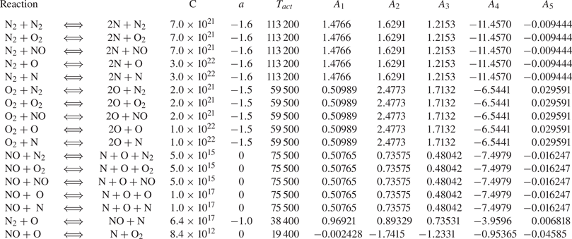
Table 5. Coefficients for computing the relaxation times  $t_m$ from Park (Reference Park1993).


 Open access