


Introduction
Recent pressure on hydrological resources caused by population influx and resource development increases the need for accurate measurement of snow-water equivalence (SWE) in alpine regions, which may produce more water per unit area than non-alpine areas (Reference Alford and Ives,Alford, 1980). In California, for example, agricultural and metropolitan areas depend on water obtained from the Sierra Nevada to augment local water supplies. Most of the run-off from the alpine regions is melt water from the seasonal snow-pack. In order to understand the timing and volume of run-off, a good appreciation of the spatial variation of snow-pack properties is needed. With the use of both established and recently developed techniques SWE measurements at a given location are not difficult to obtain. Several accurate methods for measuring density exist, ranging from those involving excavation and sampling pits (Reference Perla and MartinelliPerla and Martinelli, 1978) to the isotope-profiling gauge (Reference Kattelmann, McGurk, Berg, Bergman, Baldwin, and HannafordKattelmann and others, 1983). Depth measurement requires only a robust probe and some experience in its use.
The persistent question is: how do we accurately interpolate between measurements at points to estimate the total volume of water stored in the snow-pack over an entire drainage basin? Snow-pack properties may vary greatly over small distances and, because numerous studies have been conducted in prairies or regions of low-relief snow-pack, variation in these places is better understood than are the spatial and temporal variations of snow cover observed in alpine regions. The factors contributing to variation in SWE are slope, aspect, elevation, vegetation type, surface roughness, and energy exchange, and these are exaggerated in alpine areas, resulting in a heterogeneous snow-pack which changes markedly in space and time. Clearly, we need sampling methods which have reasonable time and manpower requirements, which accurately assess the snow-pack, and which are capable both of identifying snow-pack variability and of characterizing it over an area. An approach that requires the collecting of many samples throughout a basin is seldom practicable, given logistical constraints on safety and time.
In this study we have attempted accurately to determine the distribution of SWE over a small alpine basin based on topographic parameters that account for variations in both accumulation and ablation, by identifying and mapping zones of similar properties. These zones were calculated from a digital elevation model (DEM) with 5 m grid spacing and better than 1 m accuracy. Parameters used for this were elevation, slope, and daily integrated solar radiation for clear atmospheric conditions; snow-depth and density measurements were obtained in four intensive snow-surveys over one melt season, providing a large sample of spatial point measurements for model development and testing.
Previous Work on Snow Distribution
Investigations on snow accumulation and distribution in the last two decades have focused on elevation, vegetation, and topography. Reference MeimanMeiman (1968) summarized many of the earlier studies. Although much of the work has been done in regions of low elevation and minimum relief, many of the results obtained also apply to alpine areas. Even in regions with gentle terrain and low altitude, snow accumulation increases with elevation (Reference Steppuhn, Dyck, Santeford and SmithSteppuhn and Dyck, 1974). Studies have also examined the relationship between snow accumulation and terrain features and vegetation (Granberg, 1979). Snow accumulation has been shown to be dependent on vegetation and topographic roughness through a wide range from small-scale vegetation and surface roughness to large-scale terrain features such as ridges and valleys.
Factors Affecting Snow Distribution
In order to understand variable distribution of snow cover, it is necessary to understand the processes controlling distribution. Properties of the snow-pack such as depth, density, temperature, and chemistry vary in space and time. Snow depth and density are controlled both by accumulation and by ablation; accumulation consists of two processes: snowfall itself, and redistribution of the original snowfall by wind transport or by sloughing and avalanching. Ablation results from melting, sublimation, and deflation. Variability in both depth and density of snow must be considered in evaluations of snow distribution. Density measurements involve excavating snow pits and sampling the pit wall, which is labor-intensive and time consuming. In contrast, depth measurements simply involve probing and many samples may be taken in the time required to sample a single pit. Depth of snow varies more than its density in alpine areas, so the major source of variation in SWE is variation in depth, especially during the melt season (Reference LoganLogan, 1973). Fortunately, this makes field sampling feasible since many easily obtainable depth measurements can be combined with fewer density profiles.
Accumulation
There are several reasons for irregular snowfall in alpine environments. Although regional climate and latitude affect snowfall, neither of these varies significantly within most alpine basins. However, elevation within alpine basins may have a range of more than 1000 m and therefore elevation is considered the single most important factor in snow-cover distribution by most studies. The relationship is not independent of climate or slope, and orographic effects depend more on slope and wind speed than on elevation. Redistribution accounts for much of the spatial heterogeneity of SWE in alpine regions. Even if snowfall were uniform over an area, the final deposition pattern would be highly irregular because snow is typically moved by wind and redeposited during the precipitation event. Variation in storm patterns and wind direction further complicate the problem. Recently, much work has been done on blowing snow and this has been reviewed by Reference SchmidtSchmidt (1982a).
Like other sediments (Reference BagnoldBagnold, 1966), snow tends to accumulate in areas where air decelerates or where flow is divergent, and it tends to erode in areas of acceleration or convergent flow. Maximum drift flux on an alpine ridge is found on the up-wind side within a few metres of the crest, with scoured areas on windward slopes and deposition on lee slopes (Reference FohnFöhn, 1980; Reference SchmidtSchmidt, 1984; Reference Schmidt, Meister and GublerSchmidt and others, 1984). Deflation hollows form adjacent to objects such as trees or boulders, even when immense drifts lie nearby. Two-dimensional snow drift over simple uniform barriers is well understood and easier to model (Reference MellorMellor, 1965; Reference SchmidtSchmidt, 1980, Reference Schmidt1982b, Reference Schmidt1984; Reference Schmidt, Meister and GublerSchmidt and others, 1984). However, for the complicated three-dimensional terrain found in alpine areas, the problem of modeling is considerably more difficult and remains largely unresolved. In the short term, drifts may shift between storms as the storm track changes, although over a season consistent patterns frequently emerge.
Considerable volumes of snow may be moved by avalanches in a watershed. Regions in upper parts of basins accumulate snow in avalanche-starting zones. When released, the snow is transported down-slope to a resting point. Additional snow in the track or run-out zone may be entrained and redeposited by the moving mass. Snow may repeatedly slough from slopes if they are steep enough. Avalanching does not change the total mass of snow in a drainage basin, but correct estimates of the volume in avalanching deposits are hydrologically important because these deposits may contain large amounts of water. Reference ZalikhanovZalikhanov (1975) found that from 30 to 64% of the alpine snow cover in the Caucasus may be transported to valley bottoms by avalanches. Weir (1979)observed a single event at Mount Hutt, New Zealand, that moved about half of the SWE of the basin to an elevation well below the snow line.
Ablation
A common method of evaluating ablation and snow melt is through evaluation of the surface-energy exchange. Snow-pack ablation is controlled by energy exchanges at the air-snow and snow-ground interfaces. Of the available energy sources, it is well documented that solar and longwave radiation usually dominate (Reference Zuzel and CoxZuzel and Cox, 1975). Radiation affects net accumulation through ablation at the surface. If the melt only percolates into the snow-pack and refreezes, then depth and density have changed but SWE has not. Once melt water reaches an ice lens or the ground, however, it may move horizontally and the SWE at that point will change. Radiation thus influences the spatial element of accumulation, as it may effectively move SWE from discrete parts of the basin where the energy budget is sufficient to remove SWE when run-off leaves the basin.
In predicting areas of melt for a given set of conditions, it is necessary to examine a number of factors. Besides the basic energy-exchange components, it is necessary to consider the different physiographic characteristics of the point in question. Factors such as slope, aspect, latitude, and horizon must be taken into account, especially in rugged terrain. In high-latitude locations, where radiation inputs are low, melt and rainfall tend to have a uniform effect on thes now cover (Reference AdamsAdams, 1976). In areas where radiation is both important and variable (lower latitudes and high elevations with rough topography) variability in snow-pack parameters is increased. Some parts of alpine basins may go for 1 or 2 months in the winter without receiving direct solar radiation, while adjacent areas may receive large amounts of direct radiation and experience occasional melt throughout the winter season. In prairie or Arctic environments, where terrain features are homogeneous, a single value of irradiance can be used for the entire study area. Breaking a sub-Arctic basin into different topographic units has resulted in successful modeling of snow melt from the units using an energy-balance approach (Reference Price, and DunnePrice and Dunne, 1976). Reference Obled, Harder, Colbeck and RayObled and Harder (1979) showed that topography controlled snow distribution during the accumulation season and that it also accounted for the observed spatial diversity in snow melt during the ablation season. Rugged alpine terrain has a pronounced effect on the total energy budget, both by controlling incoming radiation and by variable emission of long-wave radiation from terrain features (Reference OlyphantOlyphant, 1984, Reference Olyphant1986a).
Study Site
The study was conducted in the Emerald Lake watershed, Sequoia National Park, California, at 36°35′N, 118°40′W (Fig. 1). Elevations range from 2780 to 2416 m, a total relief of 636 m. Total watershed area is about 120 ha, of which 2.85 ha are lake surface. The basin is a north-facing glacially scoured cirque flanked by nearly vertical cliffs on the south and west margins. A broad range of slopes and aspects is represented. The lack of soil has resulted in limited herbaceous and woody vegetation. The topography and physiography are typical of a small alpine watershed in the southern Sierra Nevada.
Field Methods
An exhaustive field program was undertaken in order to measure SWE in the Emerald Lake basin. The program resulted in hundreds of depth measurements and in the excavation of numerous pits over the basin which could be used to validate the results of the accumulation model. Sample survey points were selected randomly on a 25 m grid overlain on the 5 m resolution DEM grid. Locations of points were transferred to orthographically corrected aerial photographs which were used by the field teams, and depth measurements were taken at each accessible point. Ordinarily, a stratified random sample is preferred for statistical reasons (Reference CochranCochran, 1977); in this study, however, the survey data were used to test our classification, and stratifying the basin before the surveys were completed would have biased the results, implying pre-existing knowledge of the distribution.
Four surveys were completed, starting at the date of peak accumulation in the basin and following at 2 weekly intervals there after. The field teams used orthographic photographs, topographic maps, close-up photographs, and compasses to locate the points in the field precisely. At each location, the survey team recorded snow depth at the chosen point itself and also at positions 4 m away from each point in the four cardinal directions. The five depths were then averaged to minimize local variation of depth caused by underlying boulders. Depths were measured using interlocking aluminum probes which were suitable for up to 10 m depths. Snow pits were dug at selected sites through out the watershed in order to obtain density profiles. Locations of pit and snow-board sites are shown in Figure 1. Density of snow was measured using a 1000 cm3 stainless steel cutter and an electronic digital scale with an accuracy of 1 g. Samples were taken in 0.1 m increments to give a complete profile.

Fig. 1. Emerald Lake basin snow-pit sites. Density profiles taken at sites 2, 3, 5, 6, 7, and 8 throughout 1987 water year. Sites 1 and 4 are used for meteorological data collection. 1, tower; 2, inlet; 3, bench; 4, ridge; 5, ramp; 6, pond; 7, hole; 8, cirque.
Accumulation And Redistribution At Emerald Lake
The 1987 water year was marked by lower-than-normal precipitation. Average precipitation in California was only 65% of the 50 year mean, and estimates for the Sierra Nevada were even lower (California Cooperative Snow Survey, 1987). State-wide snow surveys showed that the snow-pack was just over 50% of normal on 1 April and 20% of the normal value on 1 May, demonstrating both low precipitation and rapid depletion of the thin snow-pack found in a dry year.
There is visible evidence for snow redistribution in the Emerald Lake watershed. Large cornices form on the uppermost ridges and face into the basin. Large storms come from the north-west and travel up the basin leaving sizeable up-slope drifts on the pronounced benches. These drifts account for a significant amount of deposition and are present in this particular watershed both in years of high and low precipitation. Similar deposits have been observed in an alpine basin in New Zealand by Reference WeirWeir (1979).
Storms in the Sierra Nevada are usually associated with air temperatures near the melting point of snow. At these high temperatures, equilibrium metamorphic processes are rapid and result in a strong well-bonded surface. During and immediately following a storm, loose snow may easily be moved and even disaggregate the old snow surface, incorporating dislodged crystals into the redistribution. Once the surface develops, little snow movement takes place even in high winds. Many of the snow patches that persist for the longest period into the melt season in the Emerald Lake watershed are avalanche deposits or snowbanks found at the foot of steep cliffs fed by sloughing from above. Depths of drifts and avalanche deposits sometimes exceeded 6 m, and sloughing from steep rock faces produced depths exceeding 8 m.
Results of Field Measurements
Snow density from field measurements
Over 50 snow pits were excavated, giving excellent density data with high spatial and temporal resolution. In the absence of strong temperature and vapour-pressure gradients in the snow-pack density increases throughout the season from overburden pressure and mixed metamorphic processes. Mean snow density showed an increase during the months from February through to June. Early season densities were low, corresponding to low temperatures and thin snow-pack but, as temperatures increased and accumulation proceeded, mean density increased asymptotically to about 470 kg m−3. The increase was rapid during the early part of the melt season and slowed down as the snow-pack matured. Data from all the pits dug in 1987 are summarized in Table I, where values represent all density measurements taken over the entire basin within 1 d of the given date. From before the date of the first survey 9 April onward, the standard deviation of the density was less than 10% of the mean in all cases, except one for which it reached 11%. A linear model was fitted, by simple correlation of the data after 1 April, in which density was a function of the day of year. Values of predicted density are also listed in Table I, and are within one standard deviation of the observed means except for the week of 27 May.
Estimations of snow-water equivalence from survey data
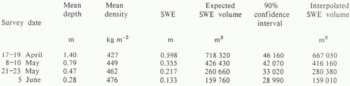
It is possible to estimate the basin SWE simply from the mean of snow depth and snow-density values obtained from surveys if the sample size is large enough. Sample size ranged from 256 to 328 during the 1987 water year, and SWE was calculated for each survey using the mean depth and density values. Statistics on the depth measurements from the four surveys are summarized in Table II. Snow-covered area was implicitly accounted for in the calculations, because the survey points without snow were averaged into the mean snow depth. The values of basin SWE calculated from this method were used to evaluate the results of basin SWE based on the classification of the basin by terrain features discussed below, and will be referred to as the expected values (Table III). Basin SWE was also calculated using Thiessen polygons following the algorithm presented by Reference RenkaRenka (1984), and volumes of water were within 8% of the expected value (Table III). Thiessen polygons and other spatial-interpolation techniques fail to account for the abrupt changes in SWE dictated by abrupt changes in the terrain. The snow-depth data exhibit low autocorrelation at all distances, which accounts for the error produced by the interpolation techniques.
Table 1. Mean basin snow density from snow pits, 1987 water year, observed and predicted weekly means
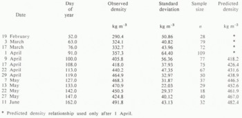
Table II. Summary of depth surveys, 1987 water year

Table III. Summary of snow-water equivalence, 1987 water year
Basin Classification
The basin was subdivided into areas of similar snow characteristics using a 5 m grid from the DEM. The large grid of 48048 points in the basin made it necessary to use digital image-processing techniques for analysis and classification. The basin was divided into regions in two steps. First, a random sample of 1000 points was drawn from the 5 m DEM. The corresponding values of radiation, slope, and elevation were clustered to identify the structure of similar groups within the basin. The entire basin was then classified using a Bayesian classifier based on the statistics generated from the clustered sub-images (Reference RichardsRichards, 1986). This technique was repeated for several variations of the parameters and for 8- and 12-class groupings. These numbers were arrived at as a compromise between their being operationally and computationally small enough and at the same time still providing adequate resolution and information. The actual number of classes varied, since the classifier omitted some classes identified by the clustering algorithm. The combinations are listed in Table IV, and for simplicity, acronyms are used for the stratifications hereafter. The acronyms include initials for each parameter used and a number corresponding to the number of classes, so that RSE12 represents radiation, slope,and elevation, with 12 classes.
Slope and radiation images were generated using Image Processing Workbench software (Reference Frew and DozierFrew and Dozier, 1986). The methods used to calculate net radiation have been described by Reference DozierDozier (1980). The three parameters were chosen because they represent physically based parameters which affect accumulation and ablation of snow. Slope and elevation are fixed in time for the purposes of this study, but radiation varies markedly through the seasons and provides the time-dependent element needed to model the change in the distribution of SWE over the basin. The net-radiation images used in the classification are indices, where the daily net radiation was calculated for a clear sky, a condition that persists in the Sierra, for the fifteenth day of each month from December through to June. These were then summed for all months before the survey date for which they were used. The radiation images for the months of December through to March and December through to June are found in Figures 2 and 3, and examination shows the marked increase in radiation through the season, particularly on the west wall of the basin. Note that the steep north-facing walls corresponding to the topographic map in Figure 1 receive low amounts of net radiation.
Table IV. Classification parameters and acronyms
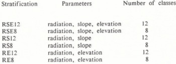

Fig. 2. Cumulative net radiation (W m−2), from December to March. Most of basin is in lower half of scale. Scale represents 1280 m.

Fig. 3. Cumulative net radiation (W m−2), December to June. Most of basin is in upper half of scale, but steep north-facing slopes and bottom of figure exhibit low net radiation values. Scale represents 1280 m.
Validation of results
Clustering and classification are not rigorous statistical techniques and formal statistical approaches for validating results do not yet exist. The results in this study have been evaluated qualitatively by our intimate knowledge of the basin and the observed snow distribution, and quantitatively by two methods. First, a single classification, ANOVA, wasused where the null hypotheses for the ANOVA was stated as: there is no difference between the means of the groups identified in the classification. If the null hypothesis is accepted, then similar information can be found in more than one class and a poor classification results. Rejection of the null hypothesis shows that the classes contain different information or represent different populations, which is the desired result. Secondly, standard errors (SE) from the classifications were compared to the basin-wide data. In any classification attempt, the SE should be reduced for the classified groups when they are compared with the whole data set, but a significant reduction in SE suggests a successful classification. All data were checked for the assumption of a normal distribution. The data for radiation, slope, and elevation were close to normal, with no hope for improvement through transformation. SWE data were normally distributed except for the many zero readings. This was partly taken care of by masking the steep snow-free areas in the basin and removing them from the statistical analysis.
Results of Classification Attempts
Scatter plots of radiation, slope, and elevation against SWE for all surveys show that the relationships are all weak, but that the correlation between SWE and radiation is the strongest. Step wise linear regression confirmed the weak relationship; radiation and slope together accounted for 40.1% of the observed variation, and inclusion of elevation made negligible improvement to 40.5%. This is the opposite of the SE results, which follow and show that elevation may be important. ANOVA results in Table V are highly significant for all classifications. Examination of the various classifications reveals some inadequacies and only the best classification result from each survey is shown. RSE12 placed the maximum accumulation low in the basin and on steep slopes, and RSE8 also has the slope problem, the remaining stratifications appear reasonable on the basis of the observed SWE; RS8 showed an increased SE over the random survey SE, RS12 places a uniform snow-pack over the entire east wall, which has not been observed. RS8 resolves the distribution problem on the east wall, but shows non-existent extensive areas of low accumulation on the west wall. RE12 (Fig. 4) gives results which appear to be reasonable, but RE8 oversimplifies the real situation and loses definition in several areas. Results for the predicted basin SWE from each classification are listed in Table VI. These values were calculated by multiplying the zone mean SWE by the zone area and summing all the zone values for the basin. All values were lower by less than 5% than the expected basin mean described earlier.
All anova results for the second survey were significant at greater than the 99% level, with the exception of RE8 which had results significant at the 96% level. RSE12 and RSE8 appear incorrectly to locate the maximum SWE at low elevation,since observations show that it should be located beneath the steep cliffs in the upper reaches of the basin where sloughs accumulate and radiation is low. RS12 (Fig. 5) and RS8 are good approximations of observed SWE distribution, but RE12 and RE8 are too coarse to be useful. Only classifications including a slope parameter improved the SE. Stepwise regression again shows radiation and slope to be the most important, although the R2 value improves substantially from 0.360 to 0.462 when elevation is included. Table VI shows that, except for RE8, all classifications over predicted SWE and that RSE12 and RE12 over predicted SWE by more than 5%.
Results from the third survey ANOVA data showed several of the classification attempts to be poor, and of the better ones only RSE8, RE12, and RE8 were significant. RSE12 locates the maximum SWE in areas of observed low accumulation, and RSE8 exhibits the same tendency to a lesser degree. RS12 (Fig. 6) and RS8 do not have this problem and correctly locate some of the large drifts found on the upper edge of steep slopes. In a purely qualitative evaluation these appear to be two of the best classifications from any of the surveys. RE12 correctly locates deposits where they linger late into the season and appears to represent observations over the entire basin. RE8 lacks definition and is too elevation-dependent. RSE8, RE12, and RE8 improved the SE. All SWE estimates fell within 5% of the basin mean except RS12. Step wise regression, for which the R2 value improved from 0.231 with radiation and slope to 0.351 with elevation, emphasized the importance of elevation.
Anova results for the fourth survey were highly significant only for RS12 and RE8. RSE12, RSE8, RS8, and RE8 do not differentiate between the western and eastern aspects of the basin, which is a result of the radiation budget becoming more uniform over the basin by this late date. RS12 does separate aspects, but locates deposits of snow poorly on the east wall of the basin. RS8 spreads the snow too evenly over the entire basin, but does correctly locate low SWE areas on the east wall. RE12 (Fig. 7) produces reasonable results and mimics observed snow cover well but lacks definition over most of the basin; it is the only classification with reduced SE. Again, stepwise regression showed the importance of all three of the earlier listed parameters; only RS12 overpredicts basin SWE by more than 5%.
Table V. Summary of anova and standard error (se) results from classification tests

Table VI. Basin swe volume estimates from classifications
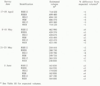
* See Table III for expected volumes.

Fig. 4. Spatial distribution of SWE in m, 17–19 April 1987 classification results from RE12. This survey and snow distribution show to maximum snow accumulation for 1987 water year. Maximum SWE is under cliffs at higher elevations, minimum SWE is on steep slopes and on eastern wall, which receives most radiation. Scale represents 1000 m.

Fig. 5. Spatial distribution of SWE in m, 8–10 May 1987 classification results from RS12. Eastern wall is becoming more uniform as more radiation received. Scale represents 1000 m.
Discussion
The results outlined above show that terrain features and radiation exert some effect on snow distribution, and also show that there is potential in modeling snow distribution in alpine areas using physically based parameters. We have shown that slope and elevation may be used as static terrain features to model SWE in this basin, and that net radiation provides a physically based, temporally dynamic variable needed to explain changing distribution through the melt season. That these three variables do not tell the whole story is evidenced by the low correlations they produce with SWE, and by the ambiguities existing in the choice of classification parameters. The large degree of the variations not explained by the regression equations also demonstrates that other additional factors control snow distribution. At this point it is not clear which scheme or parameters produce the best results; it is clear only which combinations produce poor results without the reasons for the poor results being apparent. Of the parameters used, radiation seems to be the most important since it consistently shows the highest correlation with SWE and produces the best results when only one redundant parameter is used. Slope is important because some slopes are too steep to retain snow and the slopes lying below them accumulate the sloughing snow from above. More important than slope itself may be information about neighboring slopes. Elevation is unimportant in this basin because other factors overshadow its effects, but it is suggested that its role becomes more important as the season progresses. Early in the season, elevation effects are balanced by the bare steep slopes found in the upper reaches of the basin. Later in the season, melt has been vigorous at the lower elevations, and the large deposits remaining at the bases of cliffs in the upper basin produce a stronger positive relationship between elevation and SWE.

Fig. 6. Spatial distribition of SWE in m, 21–23 May 1987 classification results from RS8. Lower elevations losing snow most rapidly, maximum SWE is at high elevations under steep cliffs where radiation is minimal. Scale represents 1000 m.

Fig. 7. Spatial distribution of SWE in m, 5 June 1987 classification results from RE12. Little snow left in entire basin. Most significant areas of remaining SWE at base of steep cliffs where sloughing during winter created deep deposits and radiation for melting is minimal. Scale represents 1000 m.
Agreement between the basin SWE volumes produced by most of the classifications and by simple statistical means is encouraging, despite the fact that it does not show which attempts are superior. Poor results would raise serious questions about the classifications. It does therefore appear that the techniques and parameters used here will generate good estimates of volume, and it is also felt that when the percentage of snow-covered area is high the method is successful at modeling the spatial distribution of SWE. As the snow-covered area is depleted, the model distributes the remaining volume of snow evenly and thinly over a large area, which is clearly not the way snow melts in rugged terrain where rapid melting of thin snow patches and persistence of discrete thick deposits have both been observed. In order for a technique to be useful to snow-melt models, it must incorporate information about snow covered area.
The technique here described may be used to design an optimal sampling scheme where the zones of similar SWE distribution are determined by areas of similar terrain features with no pre-existing information about the snow-pack. Areas containing the significant component of the total accumulation can be concentrated upon without time or energy being wasted on the less important parts of the basin. The number of samples required to describe the zone SWE to a desired level of accuracy can be determined by completing a quick on-site pilot survey. This method has obvious benefits where cost and manpower demands of other approaches would be prohibitive.
Future Work
Currently, it appears that we are doing an adequate job in modeling the change in distribution of SWE through use of the radiation index, and that we have begun to be able to explain snow accumulation through the slope and elevation variables. However, we have as yet failed effectively to model the component of accumulation caused by redistribution of the snow. We have touched on this through consideration of slope, which accounts for sloughing and persistently bare areas, but other factors in the terrain controlling redistribution must be identified. Better results may be obtained if parameters are weighted according to their apparent importance, instead of being evenly weighted or excluded altogether as has been done in this study. Variables controlling drift erosion and deposition, such as the rate of change or second derivative of slope, need to explored. Clearly, we must also use snow-covered area in future attempts at analysis if this work is to provide the accurate spatial information about SWE necessary as input to spatial snow-melt models.
Acknowledgements
This work was supported under grants by the California Air Resources Board and the University of California Water Resources Center.


