


1. Introduction
Gas transfer from bubbles to liquids is critical in multiple chemical engineering and environmental processes such as scrubbers, bubble reactors and lake oxygenation, and depends on the local flow agitation (Risso Reference Risso2018), while at the ocean surface, air entrainment by breaking waves contributes to the exchange of gases critical for the climate system (Garbe et al. Reference Garbe2014; Reichl & Deike Reference Reichl and Deike2020; Deike Reference Deike2022). Modelling approaches of bubble-mediated gas transfer in a turbulent environment require knowledge of the individual bubble mass transfer coefficient  $k_L$ (Woolf & Thorpe Reference Woolf and Thorpe1991; Keeling Reference Keeling1993; Liang et al. Reference Liang, McWilliams, Sullivan and Baschek2011; Deike & Melville Reference Deike and Melville2018).
Mass exchange related to bubble dissolution presents similarities to other heat and mass transfer problems. The classic Stefan problem (Stefan Reference Stefan1891) describes heat or mass transfer coupled with a moving boundary and was initially studied in the context of ice growth at solid–liquid interfaces (Crepeau Reference Crepeau2007). Akin to the spherical Stefan problem, Epstein & Plesset (Reference Epstein and Plesset1950) provided a quasi-stationary analytical solution to the stagnant spherical bubble dissolution. Peñas-López et al. (Reference Peñas-López, Parrales, Rodríguez-Rodríguez and Van Der Meer2016) studied the bubble growth and dissolution by removing the quasi-static radius approximation, and investigated the effect of the history term that relates to the mass transfer coupled with moving boundary. Lohse & Zhang (Reference Lohse and Zhang2015) and Zhu et al. (Reference Zhu, Verzicco, Zhang and Lohse2018) investigated a surface nano-bubble experimentally and numerically, comparing to the Epstein & Plesset (Reference Epstein and Plesset1950) results, and found that pinning of the contact line and oversaturation stabilizes the nano-bubble from dissolution.
The mass transfer from a rising bubble in a steady state (ignoring the moving boundary effect) was described by Levich (Reference Levich1962) using a thin boundary layer and potential flow assumptions around the bubble, leading to a mass transfer coefficient given by  $k_L = (2/\sqrt {{\rm \pi} })\sqrt {\mathscr {D}_l U/d}$, with $d$ the bubble diameter, $U$ the bubble rise velocity, and $\mathscr {D}_l$ the gas diffusivity in the liquid. This can be written in terms of the non-dimensional transfer rate (Sherwood number) ${Sh}=k_L d/\mathscr {D}_l$ as ${Sh} = (2/\sqrt {{\rm \pi} })\,{Pe}^{1/2}$, where ${Pe}={Re}\,{Sc}$ is the Péclet number, ${Re}=Ud/\nu _l$ is the Reynolds number, and ${Sc}=\nu _l/\mathscr {D}_l$ is the Schmidt number, with $\nu _l$ the liquid viscosity. These approximations are similar to the penetration theory (Higbie Reference Higbie1935) that is based on the fact that in unsteady heat or mass transfer, the depth of penetration into the exposed boundary is dependent on the time of contact. The longer the contact time, the deeper the penetration, and the equivalence for both theories is valid for high Péclet numbers (ratio of the rate of advective transport to the diffusive transport; Sideman Reference Sideman1966). The application of the penetration theory then relies on finding the correct time scale of contact. An experimental study on rising CO $_{2}$ bubbles by Bowman & Johnson (Reference Bowman and Johnson1962) found that the mass transfer coefficients were in close agreement with the theoretical predictions from Higbie (Reference Higbie1935) and Levich (Reference Levich1962). Takemura & Yabe (Reference Takemura and Yabe1998) developed an experimental set-up to measure the size of individual O $_{2}$ bubbles rising in silicone oil, and estimated the mass transfer coefficient with results comparable to the penetration theory. The bubbles formed at the atmosphere–ocean interface correspond to high Schmidt number ( ${Sc}\approx 600$ for CO $_{2}$ at $20\,^{\circ }$C), while the ${Sc}\ll 1$ regime occurs in liquid metals and astrophysics (Gotoh et al. Reference Gotoh, Yeung, Davidson, Kaneda and Sreenivasan2013).
A configuration of practical importance in industrial applications involves dense bubble clouds, or swarms, and requires estimations of the bubble gas transfer coefficient in this bubbly turbulent environment. Roghair (Reference Roghair2012) found that the gas transfer coefficient increases with gas hold-up (the ratio of gas volume to total volume) by numerical simulations, while experimental studies on bubble swarms (Colombet et al. Reference Colombet, Legendre, Cockx, Guiraud, Risso, Daniel and Galinat2011, Reference Colombet, Legendre, Risso, Cockx and Guiraud2015) revealed that the global gas transfer coefficient at high Schmidt numbers is described approximately by the Levich (Reference Levich1962) formula  $k_L = (2/\sqrt {{\rm \pi} })\sqrt {\mathscr {D}_l \bar {U}/d}$, considering the mean bubble rise speed $\bar {U}$ in the swarm, which is affected by turbulent fluctuations.
The mass transfer of a passive scalar at the surface of a turbulent flow has received much attention. Fortescue & Pearson (Reference Fortescue and Pearson1967) studied the absorption of CO $_{2}$ in a turbulent water flow through an open channel, and approximated the mass transfer coefficient using a large eddy model $k_L \propto (\mathscr {D}_l u_{rms}/L^\star )^{1/2}$, where $u_{rms}$ is the root-mean-square velocity of the turbulent flow. Theofanous, Houze & Brumfield (Reference Theofanous, Houze and Brumfield1976) identified two distinct mass transfer regimes for energy-containing and energy-dissipating turbulent motions, i.e. $k_L \propto (\mathscr {D}_l u_{rms}/L^\star )^{1/2}$ for low ${Re}$, and $k_L \propto (\nu _l/\mathscr {D}_l)^{-1/2} (\epsilon \nu _l)^{1/4}$ at high $Re$, where $\epsilon$ is the turbulence dissipation rate. Here, the Reynolds number is defined using a macroscopic scale allowing for comparisons between various configurations. These scalings can be written in terms of the non-dimensional transfer rate ${Sh}=k_L L^\star /\mathscr {D}_l$, where $L^{\star }$ is the integral length scale, as ${Sh} \propto ({Sc}\,{Re})^{1/2}$ (for low $Re$) and ${Sh}\propto {Sc}^{1/2}{Re}^{3/4}$ (for high $Re$). Herlina & Wissink (Reference Herlina and Wissink2016, Reference Herlina and Wissink2019) and Pinelli et al. (Reference Pinelli, Herlina, Wissink and Uhlmann2022) estimated the critical Reynolds number where this transition occurs as ${Re} \approx 500$ using numerical simulations. Lamont & Scott (Reference Lamont and Scott1970) presented experiments on mass transfer from bubbles in concurrent turbulent flows, and argued that the small-scale motions of the turbulent flow control the mass transfer, leading to $k_L \propto (\nu _l/\mathscr {D}_l)^{-1/2} (\epsilon \nu _l)^{1/4}$, corresponding to the high $Re$ regime from Theofanous et al. (Reference Theofanous, Houze and Brumfield1976). An earlier discussion of a gas bubble suspended in a turbulent liquid stream was provided by Levich (Reference Levich1962), who proposed an estimate for the gas transfer coefficient from a single bubble similar to the low $Re$ regime from Theofanous et al. (Reference Theofanous, Houze and Brumfield1976), and mentioned the difficulty of experimental verification of the theories. In Farsoiya, Popinet & Deike (Reference Farsoiya, Popinet and Deike2021), we performed direct numerical simulations of a single bubble in homogeneous isotropic turbulence for a dilute gas component (so that the bubble size did not change as it transferred gas) and bubble size in the inertial subrange. We proposed that the gas transfer coefficient scaled as ${Sh} \propto {(Sc\,Re)}^{1/2}$, comparable to the low $Re$ regime from Theofanous et al. (Reference Theofanous, Houze and Brumfield1976), with simulations performed at relatively low $Re$, without variations of the bubble size.
The importance of the topic has motivated the development of numerical methods to solve mass transfer in bubbly flows. Sato, Jung & Abe (Reference Sato, Jung and Abe2000) and Davidson & Rudman (Reference Davidson and Rudman2002) developed numerical techniques where the gas concentration is continuous across the fluid–fluid interface, while the effect of the discontinuous concentration due to solubility is considered by Bothe et al. (Reference Bothe, Koebe, Wielage, Prüss and Warnecke2004). Darmana, Deen & Kuipers (Reference Darmana, Deen and Kuipers2006) provided a three-dimensional front tracking model with mass transfer. Haroun, Legendre & Raynal (Reference Haroun, Legendre and Raynal2010) and Marschall et al. (Reference Marschall, Hinterberger, Schüler, Habla and Hinrichsen2012) presented a one-fluid formulation for the algebraic volume of fluid method. Bothe & Fleckenstein (Reference Bothe and Fleckenstein2013) introduced a two-field approach using a geometrical volume of fluid method for multicomponent conjugate mass transfer. Subgrid scale models to simulate high-Schmidt-number bubble-mediated mass exchange have been developed by Bothe & Fleckenstein (Reference Bothe and Fleckenstein2013), Weiner & Bothe (Reference Weiner and Bothe2017) and Claassen et al. (Reference Claassen, Islam, Peters, Deen, Kuipers and Baltussen2020). All the above numerical techniques do not consider local changes in volume due to gas dissolution. Recent advances in numerical methods by Tanguy et al. (Reference Tanguy, Sagan, Lalanne, Couderc and Colin2014), Fleckenstein & Bothe (Reference Fleckenstein and Bothe2015), Dodd (Reference Dodd2017), Scapin, Costa & Brandt (Reference Scapin, Costa and Brandt2020), Maes & Soulaine (Reference Maes and Soulaine2020) and Gennari, Jefferson-Loveday & Pickering (Reference Gennari, Jefferson-Loveday and Pickering2022) allow us to simulate problems of mass transfer with local volume changes.
In the present study, the initial size of the bubble is in the inertial range of the turbulent flow, and gas from the bubble dissolves in the liquid outside as the bubble volume decreases. We use an immersed boundary method based on volume penalization (Magdelaine Reference Magdelaine2019) to model the gas diffusion from the bubble. This paper is organized as follows. In § 2, we present the numerical framework and validate our approach against exact solutions of the moving interface due to dissolution in the planar and spherical geometries, and discuss the special case of the Epstein & Plesset (Reference Epstein and Plesset1950) problem. In § 3, we apply our numerical methods to study the mass transfer coefficient of a bubble dissolving while rising in quiescent water, and show that the classic Levich formula can describe the mass transfer coefficient, extended for a time-varying bubble size  $d(t)$ and velocity $U(t)$, leading to $k_L = (2/\sqrt {{\rm \pi} })\sqrt {\mathscr {D}_l\,U(t)/d(t)}$. In § 4, we study the dissolution of a single bubble in an otherwise homogeneous and isotropic turbulence flow, and show that the mass transfer coefficient can be described by ${Sh}/{Sc}^{1/2} \propto {Re}^{3/4}$, with the turbulent Sherwood number ${Sh}=k_L L^\star /\mathscr {D}_l$ and macroscale Reynolds number ${Re} = u_{rms}L^\star /\nu _l$, with $u_{rms}$ the velocity fluctuations, and $L^*$ the integral length scale. This relationship is equivalent to ${k_L}\propto {Sc}^{-1/2} (\epsilon \nu _l)^{1/4}$, showing that the smallest scales control the gas transfer in the flow, namely the Kolmogorov and Batchelor length scales.
2. Numerical framework
2.1. The Basilisk solver
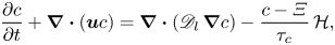
We solve the three-dimensional (3-D), incompressible, two-phase Navier–Stokes equations using the open-source solver Basilisk (Popinet Reference Popinet2009, Reference Popinet2013, Reference Popinet2015):
 $$\begin{gather} \frac{\partial \boldsymbol{u}}{\partial t}+\boldsymbol{\nabla}\boldsymbol{\cdot}(\boldsymbol{u}\boldsymbol{u})= \frac{1}{\rho}\left[-\boldsymbol{\nabla} p + \boldsymbol{\nabla}\boldsymbol{\cdot}(\mu(\boldsymbol{\nabla u}+ \boldsymbol{\nabla u}^{\rm T}))\right] + \frac{\gamma}{\rho}\,\kappa\delta_s\boldsymbol{n}, \end{gather}$$
 $$\begin{gather}\boldsymbol{\nabla}\boldsymbol{\cdot}\boldsymbol{u} = 0, \end{gather}$$
 $$\begin{gather}\frac{\partial \mathcal{T}}{\partial t} + \boldsymbol{u} \boldsymbol{\cdot} \boldsymbol{\nabla}\mathcal{T} = 0, \end{gather}$$
where  $\boldsymbol {u}$, $p$,
$p$,  $\gamma$, $\mu$, $\rho$, $\kappa$, $\boldsymbol {n}$ and $\mathcal {T}$ are the velocity, pressure, surface tension coefficient, viscosity, density, curvature, interface normal and volume fraction fields, respectively. The Dirac distribution function $\delta _s$ concentrates the surface tension force on the interface (Popinet Reference Popinet2009). The solver has been validated extensively for complex interfacial flows (Popinet Reference Popinet2015; van Hooft et al. Reference van Hooft, Popinet, van Heerwaarden, van der Linden, de Roode and van de Wiel2018; Berny et al. Reference Berny, Deike, Séon and Popinet2020; Gumulya et al. Reference Gumulya, Utikar, Pareek, Evans and Joshi2020; Farsoiya et al. Reference Farsoiya, Popinet and Deike2021; Mostert, Popinet & Deike Reference Mostert, Popinet and Deike2021; Rivière et al. Reference Rivière, Mostert, Perrard and Deike2021). It uses the projection method to compute the velocity and pressure, and the geometric volume of fluid method for the evolution of the interface between two immiscible fluids (Tryggvason, Scardovelli & Zaleski Reference Tryggvason, Scardovelli and Zaleski2011). The piecewise linear interface calculation geometric interface and flux reconstruction ensures a sharp representation of the interface (Scardovelli & Zaleski Reference Scardovelli and Zaleski1999; Marić, Kothe & Bothe Reference Marić, Kothe and Bothe2020) and is combined with an accurate height-function curvature calculation and a well-balanced, continuum surface tension model (Brackbill, Kothe & Zemach Reference Brackbill, Kothe and Zemach1992; Popinet Reference Popinet2018). Well-balanced numerical schemes ensure that specific equilibrium solutions of the (continuous) partial differential equations are recovered by the (discrete) numerical scheme. Such schemes are important when surface tension is the dominant force, such as in two-phase interfacial flows including drops or bubbles close to Laplace's equilibrium (Popinet Reference Popinet2018). Test cases by Popinet (Reference Popinet2009) demonstrate second-order convergence towards the exact circular equilibrium shape as a function of spatial resolution.
2.2. Immersed boundary method for gas diffusion
We use the numerical method developed by Magdelaine (Reference Magdelaine2019), which relies on a distributed Dirac-like forcing term, as in the immersed boundary method of Peskin (Reference Peskin1972), in order to enforce Dirichlet conditions for the gas concentration on the evolving interface. The time evolution of the gas concentration is given by
 \begin{equation} \frac{\partial c}{\partial t} + \boldsymbol{\nabla}\boldsymbol{\cdot} (\boldsymbol{u} c)=\boldsymbol{\nabla}\boldsymbol{\cdot} \left( \mathscr{D}_l\,\boldsymbol{\nabla} c \right) + F,\end{equation}
where the forcing term  $F$ relaxes the concentration toward its gas phase value on a time scale $\tau _c$ in the gas phase region $B$, and can be written as a surface integral:
 \begin{equation} F(x) = \int_{\boldsymbol{x}(s)\in B} \left(\frac{c_{g} - c}{\tau_c}\right) \delta(\boldsymbol{x}-\boldsymbol{x}(s))\,{\rm d} s, \end{equation}
where  $\delta (\boldsymbol {x})$ is a two-dimensional Dirac function, and ${{\rm d} s}$ represents the surface element of the boundary (Peskin Reference Peskin1972). Equation (2.4) can then be re-expressed as
 \begin{equation} \frac{\partial c}{\partial t} + \boldsymbol{\nabla}\boldsymbol{\cdot} (\boldsymbol{u} c)=\boldsymbol{\nabla}\boldsymbol{\cdot} \left(\mathscr{D}_l\,\boldsymbol{\nabla} c \right) - \frac{c - c_g}{\tau_c}\,\mathcal{H}(\boldsymbol{x}). \end{equation}
Here,  $\mathcal {H}(\boldsymbol {x}) = \int _{-\infty }^{0} \delta (\boldsymbol {x} - \boldsymbol {x}(s))\,{{\rm d} s}$ is a (surface) Heaviside function for the non-diffusive phase (gas phase) with the relaxation time scale $\tau _c= 10^{-6} \varDelta ^2/\mathscr {D}_l$, with $\varDelta$ the grid size. The relaxation time scale needs to be small enough to ensure an accurate imposition of the Dirichlet condition on the interface, while being large enough to avoid possible amplification of round-off errors.
The assumption of continuous chemical potentials, which is good for most applications at an interface  $\varSigma (t)$, results in Henry's law (Bothe & Fleckenstein Reference Bothe and Fleckenstein2013):
 \begin{equation} c_{l} = c_{g} \alpha\quad \text{at}\ \varSigma(t), \end{equation}
where the dimensionless ratio of the liquid phase concentration to the gas phase concentration of the component transferred,  $\alpha$, is Henry's law solubility constant (solubility hereafter). We consider a single component and an isothermal configuration, and there is no bubble break-up or large deformation of the interface that can change the pressure inside the bubble significantly. Hence the solubility, which depends on temperature, pressure and mole fraction of the gas components (Bothe & Fleckenstein Reference Bothe and Fleckenstein2013), is assumed to be constant. We modify the last term in (2.4) to account for the solubility:
 \begin{equation} \frac{\partial c}{\partial t} + \boldsymbol{\nabla}\boldsymbol{\cdot} (\boldsymbol{u} c)=\boldsymbol{\nabla}\boldsymbol{\cdot} \left( \mathscr{D}_l\,\boldsymbol{\nabla} c \right) - \frac{c - \varXi}{\tau_c}\,\mathcal{H},\end{equation}
where  $\varXi$ is a conditional variable equal to $\alpha c_{g}$ and $c_{g}$ in the interfacial and non-interfacial cells, respectively. The gradients of $c$ are calculated using central differences, and the Heaviside function is approximated as $1 - \mathcal {T}$.
The advection and diffusion terms in (2.8) are treated in a time-split manner. For diffusion we use a time-implicit Euler discretization
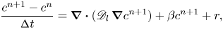 \begin{equation} \frac{c^{n+1}-c^{n}}{{\rm \Delta} t} =\boldsymbol{\nabla}\boldsymbol{\cdot} ( \mathscr{D}_l\,\boldsymbol{\nabla} c^{n+1} ) + \beta c^{n+1} + r, \end{equation}
where  $\beta = - \mathcal {H}/\tau _c$ and $r = -\mathcal {H}\varXi /\tau _c$. Equation (2.9) gives a set of linear equations that are solved efficiently using the multigrid method (Popinet Reference Popinet2015).
The solubility boundary condition (2.7) presents a discontinuity for the concentration field across the interface similar to the volume fraction field  $\mathcal {T}$. As discussed by Bothe & Fleckenstein (Reference Bothe and Fleckenstein2013), when the mass transfer is coupled with fluid flow, the concentration discontinuity given by Henry's law must be satisfied at the fluid–fluid interface. Moreover, the advection of the concentration field $c$ must be consistent with the advection of the volume fraction field since any relative motion would lead to artificial mass transfer across the interface. To avoid this numerical diffusion across the interface, we use the two-scalar approach for advection proposed by López-Herrera et al. (Reference López-Herrera, Ganan-Calvo, Popinet and Herrada2015), i.e. two tracer fields $\phi _{g}$ and $\phi _{l}$ associated with the volume of fluid $\mathcal {T}$ are defined:
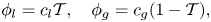 $$\begin{gather} \phi_l = c_l \mathcal{T},\quad \phi_g= c_g(1-\mathcal{T}), \end{gather}$$
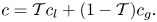 $$\begin{gather}c = \mathcal{T} c_l + (1 - \mathcal{T})c_g. \end{gather}$$
Using (2.7) and (2.11), we get
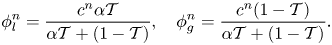 \begin{equation} \phi^n_{l} = \frac{c^{n}\alpha \mathcal{T}}{\alpha \mathcal{T}+(1-\mathcal{T})},\quad \phi^n_{g} = \frac{c^{n}(1-\mathcal{T})}{\alpha \mathcal{T}+(1-\mathcal{T})}. \end{equation}
The advection equation for  $\phi _{g/l}$ reads
 \begin{equation} \frac{\partial \phi_{g/l}}{\partial t} + \boldsymbol{\nabla} \boldsymbol{\cdot} (\boldsymbol{u} \phi_{g/l})=0, \end{equation}
and is solved using the volume-of-fluid associated fields (López-Herrera et al. Reference López-Herrera, Ganan-Calvo, Popinet and Herrada2015; Farsoiya et al. Reference Farsoiya, Popinet and Deike2021) that guarantee strictly non-diffusive transport close to the interface. The concentration tracer is updated after advection using
 \begin{equation} c = \phi_{g} + \phi_{l}. \end{equation}
 We then calculate the dissolution velocity at the interface,  $\boldsymbol {u}^\varSigma$, which is used to update the volume fractions (Magdelaine Reference Magdelaine2019):
 \begin{equation} \frac{\partial \mathcal{T}}{\partial t} + \boldsymbol{u}^\varSigma \boldsymbol{\cdot} \boldsymbol{\nabla}\mathcal{T} = 0.\end{equation}
The boundary condition for molar mass flux at an interface is given by (Fleckenstein & Bothe Reference Fleckenstein and Bothe2015)
 \begin{equation} [[c (\boldsymbol{u} - \boldsymbol{u}^\varSigma)]]\boldsymbol{\cdot} \boldsymbol{n} + [[\,\boldsymbol{j}]] \boldsymbol{\cdot} \boldsymbol{n}_\varSigma = 0, \end{equation}
where  $\boldsymbol {u}$ and $\boldsymbol {u}^\varSigma$ are the barycentric and interface velocities, respectively.
The Stefan currents from a dissolving bubble can be estimated from the source term in the continuity equation. They are discussed by Dodd (Reference Dodd2017) in the context of evaporating droplets in homogeneous and isotropic turbulence (HIT) flow
 \begin{equation} \boldsymbol{\nabla}\boldsymbol{\cdot} \boldsymbol{u}=\frac{1}{Pe} \left(\frac{\boldsymbol{\nabla} Y_v\boldsymbol{\cdot} \boldsymbol{n}\,\delta(n)}{1-Y_{v}} \right) \left(1 -\frac{\rho_g}{\rho_{l}}\right), \end{equation}
where  $Y_v$ is the mass fraction of the vapour. The numerical simulations performed for the bubble in turbulent flow are in the region $\rho _g \ll \rho _l$ ( $\rho _l/\rho _g = 850$) and ${Pe}\gg 1$ ( $80 \lessapprox {Pe} \lessapprox 5\times 10^4$), the Péclet number being defined based on some characteristic velocity of the flow. Hence the Stefan currents are small compared to the flow around the bubble. In addition, the vapour recoil and surface tension typical of air bubbles dissolution in water scale as $(\rho _g(\boldsymbol {u}-\boldsymbol {u}^{\varSigma })\boldsymbol {\cdot } \boldsymbol {n}_{\varSigma })^{2} ({1}/{\rho _g}) \approx {O}(10^{-6})$ and $\gamma \kappa \approx O(10^2)$, respectively. These forces can be comparable for the cases of strong evaporation of a droplet and cavitation of a bubble (Fleckenstein & Bothe Reference Fleckenstein and Bothe2015), which is not the case in our study. Consequently, Stefan currents and vapour recoil are not included in the present numerical framework.
As the Stefan currents are not modelled, the interface velocity  $\boldsymbol {u}^\varSigma$ from (2.16) reduces to
 \begin{equation} \boldsymbol{u}^\varSigma = \frac{M_w}{\rho_g (1 - \alpha)}\,\mathscr{D}_l\,\boldsymbol{\nabla} c, \end{equation}
where  $M_w$ is the molecular mass of the gas. The time step is not restricted by the scalar diffusion terms as we are using an implicit discretization for diffusion terms. However, fast diffusion calculates the phase change interface velocity, which restricts the time step, and the interfacial velocity $\boldsymbol {u}^\varSigma$ restricts the computational time step in accordance with Courant–Friedrichs–Lewy criteria.
Moreover, this approach is convenient in simulating HIT flows as these require periodic conditions on the computational domain boundaries, and having a source term in the continuity equation is then needed to be compensated for the extra liquid inside the domain. We thus assume that the solvent is an infinite reservoir, and study the bubble dissolution in an HIT flow. Note also that there are methods developed by Fleckenstein & Bothe (Reference Fleckenstein and Bothe2015), Malan (Reference Malan2018), Scapin et al. (Reference Scapin, Costa and Brandt2020) and Maes & Soulaine (Reference Maes and Soulaine2020) for inclusion of Stefan currents. A recent independent development by Gennari et al. (Reference Gennari, Jefferson-Loveday and Pickering2022) in Basilisk based on the two-scalar approach by Fleckenstein & Bothe (Reference Fleckenstein and Bothe2015) treats the velocity discontinuity at the interface that is due to the mass transfer between the phases.
2.3. Validation
2.3.1. Stefan problem
We test our methods with the classical moving boundary problem, called the Stefan problem (Stefan Reference Stefan1891) in planar geometry, where the liquid and gas phases are separated by a moving interface  $Y(t)$. The concentration of gas in the liquid phase (neglecting the advection) is given by
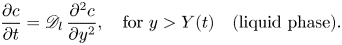 \begin{equation} \frac{\partial c}{\partial t} = \mathscr{D}_l\,\frac{\partial^2 c}{\partial y^2},\quad \text{for}\ y > Y(t) \quad \text{(liquid phase)}. \end{equation}
The moving interface concentration is constant:
 \begin{equation} c(Y(t),t) = \alpha c_g,\quad t \geq 0, \end{equation}
and
 \begin{equation} c(y\rightarrow \infty,t) = 0,\quad c(y > Y(t),0) = 0, \end{equation}
where  $\alpha$ is Henry's solubility constant, and $c_g$ is the gas concentration in the gas phase. The problem can be non-dimensionalized using the characteristic length $L$,
$L$,  $\zeta = (y-Y(0))/L$, the time as a mass Fourier number ${Fo}_m = \mathscr {D}_l /L^2t$, the moving boundary $\varSigma ({Fo}_m) = (Y(t)-Y(0))/L$, and the concentration $\varTheta = c(y,t)/(\alpha c_g)$, so that
 \begin{equation} \frac{\partial \varTheta}{\partial {Fo}_m} = \frac{\partial^2 \varTheta}{\partial \zeta^2},\quad \text{for}\ \zeta > \varSigma({Fo}_m) \quad \text{(liquid phase)}. \end{equation}
The moving interface concentration is constant:
 \begin{equation} \varTheta(\varSigma,\textrm{Fo}_m) = 1,\quad {Fo}_m \geq 0. \end{equation}
The velocity of the moving interface from (2.16),  $Y(t)$, is given by
 \begin{equation} \frac{{\rm d} \varSigma}{{\rm d} Fo} = {St}\left(\frac{\partial \varTheta}{\partial \zeta}\right)_{\zeta = \varSigma({Fo}_m)},\quad {Fo}_m > 0, \end{equation}
with conditions
 \begin{equation} \varTheta(\zeta \rightarrow \infty,t) = 0,\quad \varSigma(0) = 0,\quad \varTheta(\zeta > 0,0) = 0, \end{equation}
and Stefan number
 \begin{equation} {St} = \frac{\alpha }{1- \alpha}. \end{equation}
The time evolution of the interface and concentration is given by (Alexiades & Solomon Reference Alexiades and Solomon2018)
 $$\begin{gather} \varSigma({Fo}_m) = 2\lambda \sqrt{{Fo}_m}, \end{gather}$$
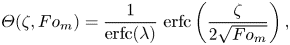 $$\begin{gather}\varTheta(\zeta,{Fo}_m) = \frac{1}{\operatorname{erfc}(\lambda)}\,\operatorname{erfc}\left(\frac{\zeta}{2\sqrt{{Fo}_m}}\right), \end{gather}$$
where  $\lambda$ is the solution of the equation
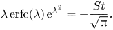 \begin{equation} \lambda \operatorname{erfc}({\lambda})\,{\rm e}^{\lambda^2} ={-}\frac{St}{\sqrt{\rm \pi}}. \end{equation}
Comparing the integration of concentration profile (2.28),
 \begin{equation} \int_{\varSigma({Fo}_m)}^\infty \varTheta(\zeta,{Fo}_m)\,{\rm d}\zeta = \int_0^\infty \left[\frac{1}{\operatorname{erfc}(\lambda)}\, \operatorname{erfc}\left(\frac{\zeta}{2\sqrt{{Fo}_m}}\right)\right]{\rm d}\zeta ={-}2\lambda \sqrt{{Fo}_m}, \end{equation}
with (2.27) shows that the solution conserves mass. Note that (2.27) (displacement of interface) and (2.30) (mass of gas) have negative and positive signs, respectively ( $\lambda <0$).
The test simulation is performed in a two-dimensional square box with  ${St} = 0.8$, with an adaptive resolution of 2048 cells per side of the domain. The position of the interface with time is shown in figure 1(a), and the concentration of gas in the liquid at a location in the domain is shown in figure 1(b). Both quantities show good agreement with the theoretical predictions (2.27) and (2.28), respectively. In figure 1(c), the net mass of gas is conserved, and liquid side mass shows good agreement with (2.30). Figures 1(d,e) show first-order convergence of the numerical methods. The agreement is good throughout the full time and space evolution.
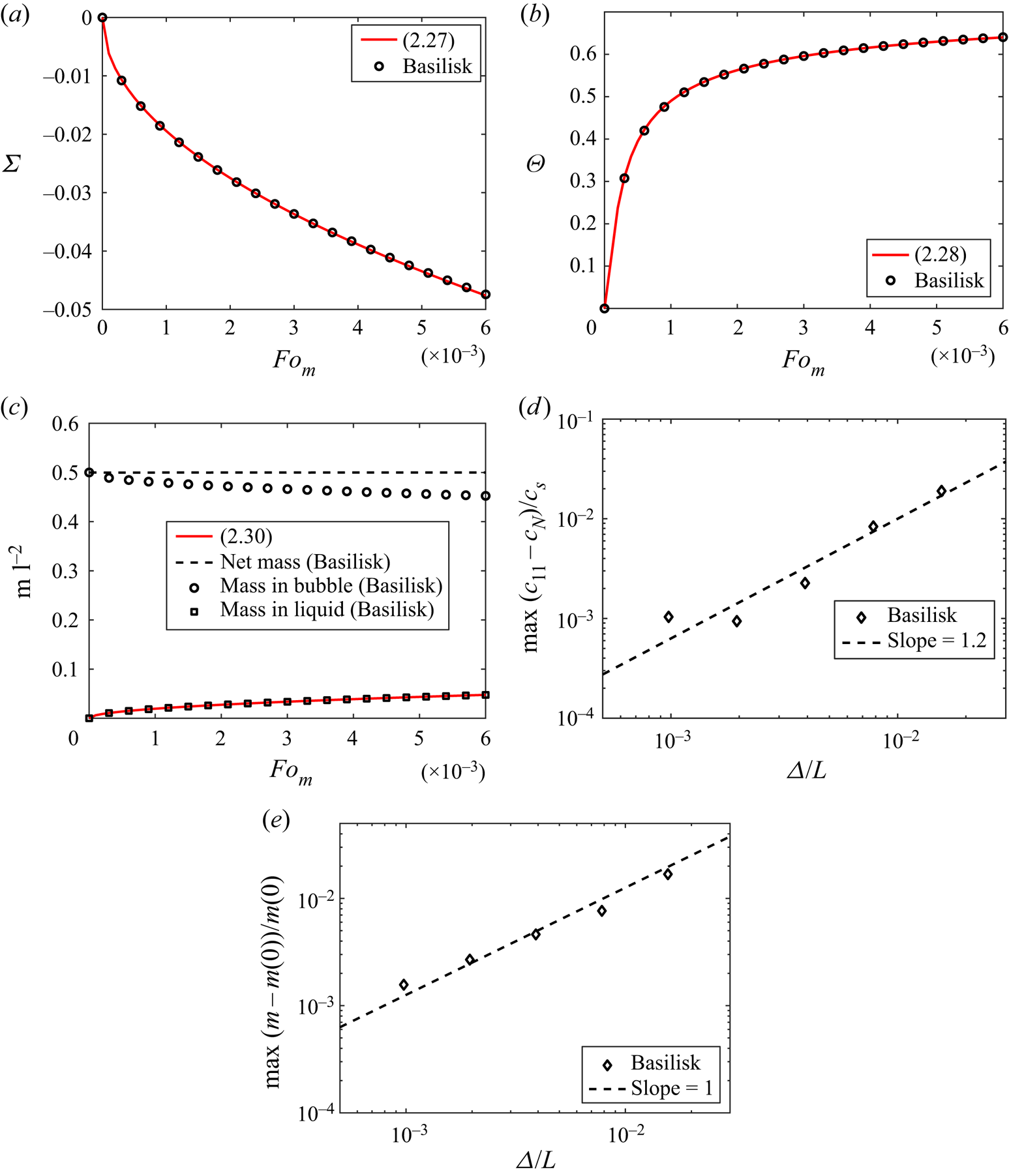
Figure 1. Test results for the planar Stefan problem, for  $St=0.8$ and grid size $(2^{11})^2$ (adaptive). (a) The interface position shows good agreement with (2.27). (b) Concentration at $\zeta = 0.02$ shows good agreement with (2.28). (c) Gas mass is conserved and shows good agreement with (2.30). The scripts for the test cases are available; see Farsoiya, Popinet & Deike (Reference Farsoiya, Popinet and Deike2022a). (d) Maximum relative error at different resolutions, $\max |c_{11}-c_N|/c_{s}$, where $c_{11}$ and $c_N$ are numerical solutions at resolution $2^{11}$ and lower, respectively, displaying first-order convergence. (e) Maximum relative error in mass conservation at different resolutions, $\max |m(t)-m(0)|/m(0)$, where $m(t)$ and $m(0)$ are net mass (time evolution) and initial net mass, displaying first-order convergence.
2.3.2. Dissolution of a static spherical bubble
We now apply our numerical methods to the dissolution of a static spherical bubble. The gas diffusion in the liquid phase outside a spherical bubble, neglecting advection, is governed by
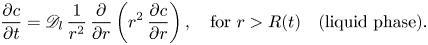 \begin{equation} \frac{\partial c}{\partial t} = \mathscr{D}_l\,\frac{1}{r^2}\, \frac{\partial}{\partial r}\left(r^2\,\frac{\partial c}{\partial r}\right),\quad \text{for}\ r > R(t) \quad \text{(liquid phase)}. \end{equation}
The moving interface concentration is constant:
 \begin{equation} c(R(t),t) = \alpha c_g,\quad t \geq 0, \end{equation}
and  $c(r \rightarrow \infty,t) \rightarrow 0$, where $\alpha$ is Henry's solubility constant, and $c_g$ is the gas concentration in the gas phase. The velocity of the moving interface $R(t)$ from (2.16) is given by
 \begin{equation} \frac{{\rm d} R(t)}{{\rm d} t} = \frac{\mathscr{D}_l}{c_g(1-\alpha)} \left(\frac{\partial c}{\partial r}\right)_{r = R(t)},\quad t > 0, \end{equation}
with initial conditions  $R(0) = R_0$ and $c(r > R_0,0) = 0$. We consider the configuration for a large driving force for transport given by a large Stefan number (which will apply in particular to larger solubility), here ${St} = 0.8$. At this Stefan number, the change in bubble size affects the diffusion of gas $({St} \sim O(1))$ over time. We solve numerically (forward Euler method) the moving boundary problem given by (2.31)–(2.33) (numerical moving boundary problem, NMBP). The concentration $c$ and bubble radius $R(t)$ can be non-dimensionalized as $\varTheta = c(r,t)/(\alpha c_g)$ and $\epsilon =R(t)/R_0$ (2.36a–c).
The non-dimensional bubble radius is shown in figure 2(a), and the concentration at a location outside the bubble at  $r = R_0 + 0.2$ is shown in figure 2(b). Good agreement is found with the numerical solution to the moving boundary problem. Figure 2(c) illustrates the mass conservation properties. The numerical method is robust in keeping the shape of the shrinking bubble nearly spherical, as shown in figure 2(d), with the sphericity $\varPsi = {\rm \pi}^{1/3}(6V_b)^{2/3}/A_b$, where $V_b$ and $A_b$ are the volume and area of the bubble, respectively. As the bubble shrinks, the number of cells per diameter decreases, and the amplitude of the oscillations in sphericity increases, which is expected.
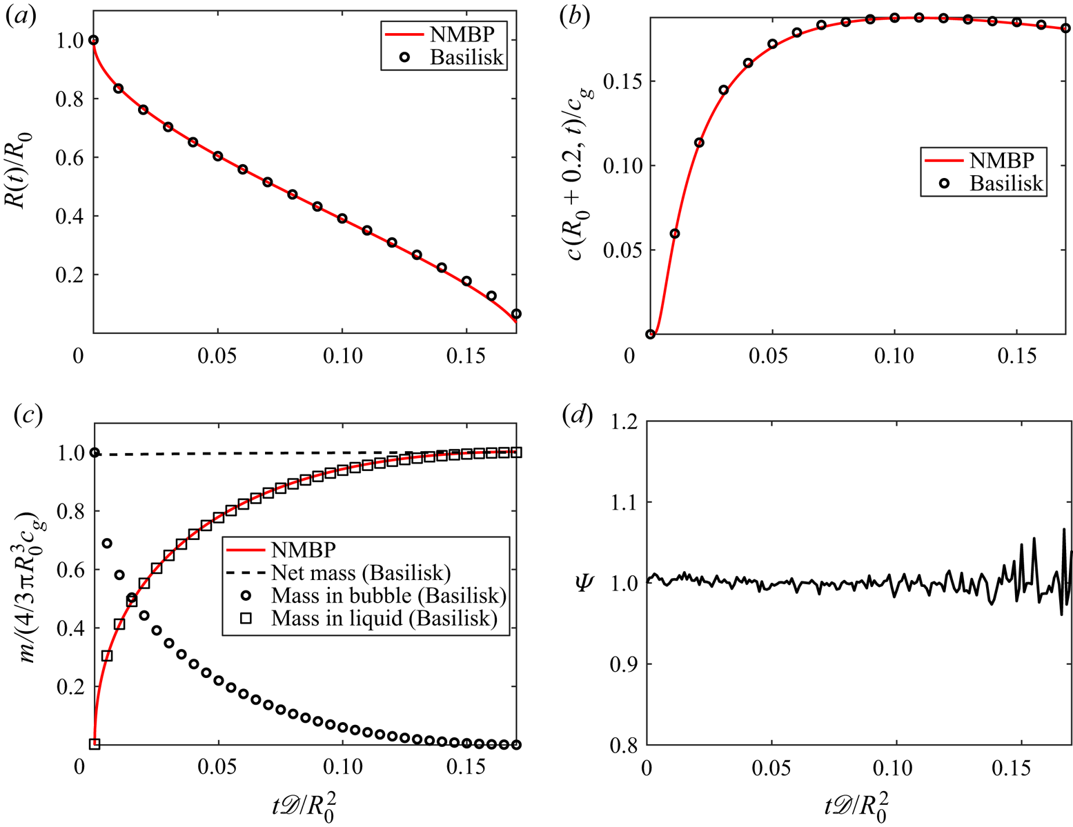
Figure 2. Dissolution of a static bubble in the high- $St$-regime ( $St =4$) large driving force for transport. Grid size 200 cells per initial diameter. (a) Time evolution of bubble radius. (b) Concentration at $r = R_0 + 0.2$ shows good agreement with numerical solution of the moving boundary problem given by (2.31)–(2.33). (c) The net mass of gas is conserved, and the evolution of the mass of gas dissolved in the liquid agrees with the volume integration of $c$ (NMBP). (d) Sphericity remains close to unity as the bubble shrinks.
2.3.3. Epstein–Plesset test
Epstein & Plesset (Reference Epstein and Plesset1950) provided an analytical solution on the dissolution of a spherical bubble under the quasi-static radius approximation (Weinberg & Subramanian Reference Weinberg and Subramanian1980; Peñas-López et al. Reference Peñas-López, Parrales, Rodríguez-Rodríguez and Van Der Meer2016), i.e. treating the bubble radius as a constant at the concentration boundary condition at the interface. It is valid if the motion of the interface is much slower than the diffusion process. The Epstein & Plesset (Reference Epstein and Plesset1950) test and approximations have been discussed in Duncan & Needham (Reference Duncan and Needham2004), Peñas-López et al. (Reference Peñas-López, Parrales, Rodríguez-Rodríguez and Van Der Meer2016), Chu & Prosperetti (Reference Chu and Prosperetti2016) and Zhu et al. (Reference Zhu, Verzicco, Zhang and Lohse2018).
Under these approximations, the time evolution of the interface is given by Epstein & Plesset (Reference Epstein and Plesset1950) as
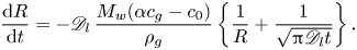 \begin{equation} \frac{{\rm d} R}{{\rm d} t}={-}\mathscr{D}_l\,\frac{M_w(\alpha c_g - c_0)}{\rho_g} \left\{\frac{1}{R}+\frac{1}{\sqrt{{\rm \pi} \mathscr{D}_l t}}\right\}. \end{equation}
In dimensionless form,
 \begin{equation} \frac{{\rm d}\epsilon}{{\rm d}x} ={-}\frac{x}{\epsilon} - 2\xi, \end{equation}
where
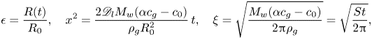 \begin{equation} \epsilon = \frac{R(t)}{R_0},\quad x^2 = \frac{2 \mathscr{D}_l M_w (\alpha c_g - c_0)}{ \rho_g R_0^2}\,t,\quad \xi = \sqrt{\frac{M_w(\alpha c_g - c_0)}{2{\rm \pi} \rho_g}} = \sqrt{\frac{St}{2{\rm \pi} }}, \end{equation}
where  ${St}$ is the Stefan number. The solution of (2.35) is given in the parametric form
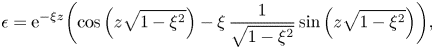 $$\begin{gather} \epsilon = {\rm e}^{-\xi z} \biggl(\cos \left(z\sqrt{1-\xi ^2} \right)-\xi\, \frac{1}{\sqrt{1-\xi ^2}} \sin \left(z\sqrt{1-\xi ^2} \right)\biggr), \end{gather}$$
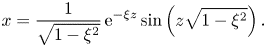 $$\begin{gather}x =\frac{1}{\sqrt{1-\xi^2}}\,{\rm e}^{-\xi z} \sin \left(z\sqrt{1-\xi ^2} \right). \end{gather}$$
 The analytical solution of (2.31) (Darmana et al. Reference Darmana, Deen and Kuipers2006) can be used for a quasi-static boundary  $R(t)$ to get the concentration as
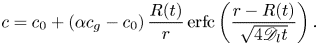 \begin{equation} c = c_0 + (\alpha c_g - c_0)\,\frac{R(t)}{r} \operatorname{erfc}\left( \frac{r - R(t)}{\sqrt{4 \mathscr{D}_l t}} \right). \end{equation}
 We set up a test case to mimic the Epstein & Plesset (Reference Epstein and Plesset1950) conditions by considering  $u^\varSigma _{EP} = 2\times 10^{-4}u^\varSigma$ in (2.18), valid for a quasi-stationary bubble. This approximation creates a mass source and hence does not conserve the total mass of the gas. The test is performed with an adaptive local resolution of 200 cells per initial diameter. The diffusivity $\mathscr {D}_l$ non-dimensionalizes the time as a Fourier number ${Fo}_m = \mathscr {D}_l/R_0^2 t$, while the non-dimensional spatial variable can be written as $x^2 = 2\,{Fo}_m\,{St}$. The motion of the bubble boundary in figure 3(a) shows good agreement with (2.37a), (2.37b). Figure 3(b) shows good agreement of the concentration at $r = R_0 + 0.2$ with (2.38). The good agreement is observed for most of the time evolution of the bubble dissolution, with small deviations at later times related to the quasi-stationary approximation by Epstein & Plesset (Reference Epstein and Plesset1950). This validates our numerical implementation in the configuration considered by Epstein & Plesset (Reference Epstein and Plesset1950).
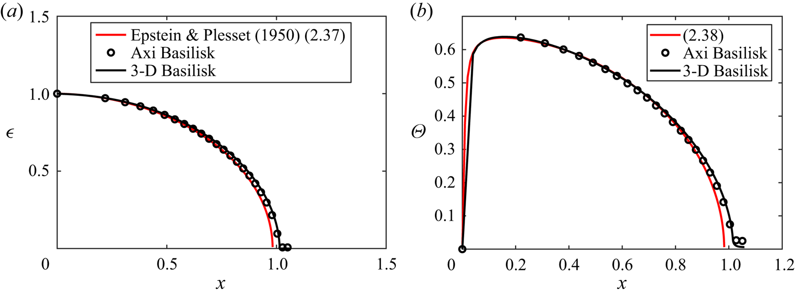
Figure 3. Dissolution of a static bubble in the quasi-stationary approximation  $u^\varSigma _{EP} = 2\times 10^{-4}u^\varSigma$. The grid size is 200 cells per initial diameter. (a) The time evolution of the bubble radius shows good agreement with (2.37a), (2.37b). (b) Concentration $\varTheta = (c(r,t) - \alpha c_g)/(c_0 - \alpha c_g)$ at $r = R_0 + 0.2$, in good agreement with (2.38). Scripts for test cases are available; see Farsoiya, Popinet & Deike (Reference Farsoiya, Popinet and Deike2022b).
3. Dissolution of a rising bubble
After considering the cases of static bubbles dissolving in a liquid, we now consider the effects of advection and the case of a bubble rising and dissolving in an initially quiescent liquid. The bubble is initially spherical and rises due to buoyancy while shrinking due to the dissolution of gas. Levich (Reference Levich1962) proposed a model for the gas transfer velocity from a bubble rising with terminal velocity  $U$ as $k_L = 2\sqrt {\mathscr {D}_l U/{\rm \pi} d}$, assuming a spherical shape and a constant size and surface concentration. Legendre & Magnaudet (Reference Legendre and Magnaudet1999) obtained a similar result for a steady axisymmetric straining flow mass transfer coefficient ${Sh} = 2\sqrt {Pe_0/{\rm \pi} }$. This relationship considers a steady state with a constant terminal velocity and does not account for changes in bubble size; hence it is valid in the limit of exchange of dilute components from the bubble, and we have verified this result previously for a constant bubble size (Farsoiya et al. Reference Farsoiya, Popinet and Deike2021).
We propose to extend the formula from Levich (Reference Levich1962) to the case of a bubble changing its size and associated rising velocity, writing
 \begin{equation} k_L(t) = \frac{2}{\sqrt{\rm \pi}}\sqrt{\frac{\mathscr{D}_l\,U(t)}{d(t)}}, \end{equation}
where  $U(t)$ and $d(t)$ are the now time-varying rise velocity and equivalent bubble diameter of a sphere having the same volume.
We compare this model against numerical simulations of a bubble rising in an initially quiescent liquid and shrinking in size due to dissolution, leading to a time-varying rise velocity  $U(t)$, and instantaneous size $d(t)$. We define the non-dimensional mass transfer coefficient (or Sherwood number) ${Sh}=k_L(t)d_0/\mathscr {D}_l$, while the specific bubble rise configuration can be defined by the bubble Morton number ${Mo} = {g \mu _l^4}/{(\rho _l \gamma ^3)}$ and Bond number ${Bo} = {\rho _l g d_0^2}{\gamma }$ (Moore Reference Moore1965; Maxworthy et al. Reference Maxworthy, Gnann, Kürten and Durst1996; Clift, Grace & Weber Reference Clift, Grace and Weber2005; Cano-Lozano et al. Reference Cano-Lozano, Martinez-Bazan, Magnaudet and Tchoufag2016).
Figures 4(a–d) show a bubble rising for given Morton and Bond numbers. The bubble is resolved with up to 200 cells per diameter. The values of  $Mo$ and $Bo$ are chosen from Farsoiya et al. (Reference Farsoiya, Popinet and Deike2021) and Deising, Marschall & Bothe (Reference Deising, Marschall and Bothe2016). In figures 4(a–d), we observe the bubble rising and shrinking in size, as well as the associated wake of gas left behind.
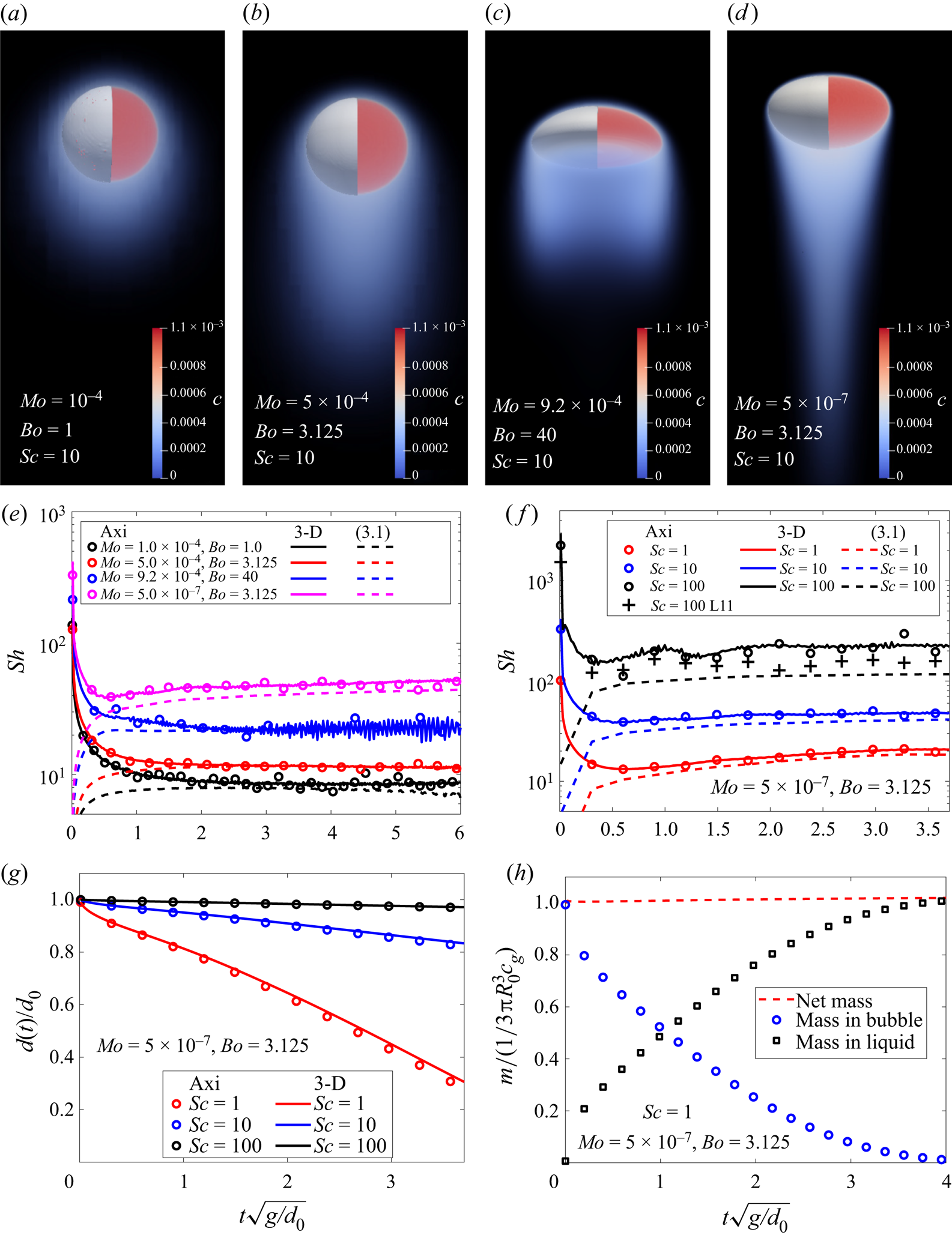
Figure 4. (a–d) Interface of a 3-D bubble (white, only left half shown in order to see the concentration field of gas inside the bubble) for various  $Mo$ and $Bo$ (specified in the keys). (e) Non-dimensional mass transfer coefficient $Sh = k_L(t) d_0/\mathscr {D}_l$ as a function of time $t\sqrt {g/d_0}$ for the four cases shown in (a–d). ( f) Coefficient $Sh$ as a function of time for increasing $Sc=1,10,100$, at $Mo =5\times 10^{-7}$ and $Bo =3.125$, and corresponding curves for (3.1), using the instantaneous bubble size and velocity. (g) Time evolution of the bubble diameter for varying $Sc=1,10,100$, for $Mo=5\times 10^{-7}$ and $Bo =3.125$. Good agreement between the axisymmetric and 3-D simulations is observed. (h) Net gas mass is conserved until the bubble dissolves completely ( $Sc=1$, $Mo=5\times 10^{-7}$ and $Bo=3.125$).
The total mass  $N$ and average gas concentration $\bar {c}$ inside and outside the bubble is computed as
 \begin{equation} {N}_{g} =\int_{V_g}c\,{\rm d} V,\quad {N}_{l} = \int_{V_l}c\,{\rm d} V,\quad \bar{c}_{g} = \frac{1}{V_g} \int_{V_g}c\,{\rm d} V,\quad \bar{c}_{l} = \frac{1}{V_l} \int_{V_l}c\,{\rm d} V, \end{equation}
where  $V_g$ and $V_l$ are the volumes of bubble and liquid, respectively. Given that the gas does not leave the domain, the mass transfer coefficient $k_L$ is calculated as
 $$\begin{gather} k_L = \frac{1}{A_g(\alpha c_g - c_l)}\,\frac{{\rm d} N}{{\rm d} t},\quad \text{or}\quad k_L=\frac{{N}_{l}^{n+1}-{N}_{l}^n}{A_g\,{\rm \Delta} t\,(\alpha \bar{c}_{g}^{n+1/2}-\bar{c}_{l}^{n+1/2})}, \end{gather}$$
where  $A_g$ is the instantaneous surface area of the bubble.
Figures 4(e, f) show the time evolution of the non-dimensional transfer coefficient  ${Sh}$ from the simulations. Good agreement with (3.1) is observed. Figure 4(g) shows the time evolution of the diameter of the bubble for both axisymmetric and 3-D simulations. Figure 4(h) shows that the net mass of gas is conserved as the bubble gets dissolved completely in the liquid.
We note that the gas bubble has shrunk more for the initial volume at a lower Schmidt number as it corresponds to a gas with higher diffusivity. The formula (3.1) works when provided with the instantaneous rise velocity and size of the bubble. Therefore, we expect that it would apply to a wide range of initial bubble configurations, defined by the bubble Bond and Morton numbers, including configurations at higher Reynolds numbers with spiralling or zigzagging bubble trajectories. The increase in diffusivity  $\mathscr {D}_l$ increases the diffusion of gas from the bubble. Higher solubility $\alpha$ gives higher concentration at the bubble boundary and results in a higher concentration gradient and higher gas transfer. The Stefan number is $O(1)$ and does not affect (3.1) for the high Péclet regime.
4. Bubble dissolution in HIT flow
We now present direct numerical simulations of bubble dissolution in HIT. First, we perform a precursor simulation to achieve a stationary HIT state, and then we insert the bubble. The methodology is similar to the preceding work on bubble deformation (Perrard et al. Reference Perrard, Rivière, Mostert and Deike2021), break-up (Rivière et al. Reference Rivière, Mostert, Perrard and Deike2021) and dilute gas transfer (Farsoiya et al. Reference Farsoiya, Popinet and Deike2021). A similar approach has been taken in independent studies by Loisy & Naso (Reference Loisy and Naso2017), Dodd & Ferrante (Reference Dodd and Ferrante2016) and Dodd et al. (Reference Dodd, Mohaddes, Ferrante and Ihme2021). Naso & Prosperetti (Reference Naso and Prosperetti2010) have observed an unstable behaviour in such a configuration when coupling to a rigid sphere. Such instability is specific to the two-way coupling with rigid (non-deformable) particles with a density close to that of the carrying fluid, and is not observed in deformable bubbles and droplets. The methodology is summarized briefly for completeness.
4.1. Precursor simulation
A cubic domain of size  $L$ periodic in all three dimensions is subjected to linear volumetric forcing $f = A\,\boldsymbol {u}(\boldsymbol {x},t)$ (Lundgren Reference Lundgren2003) in (2.1). Rosales & Meneveau (Reference Rosales and Meneveau2005) have demonstrated that this leads to a turbulent field with similar statistics to that obtained with a spectral code, and leads to a well-characterized HIT flow. We use adaptive mesh refinement on the velocity field, and the maximum level of refinement can be used to compare the resolution with that of a fixed grid. The domain consists of fluid of density $\rho _l$ and viscosity $\mu _l$. The turbulent flow is generated for increasing resolutions, with the maximum level of refinement going from 6 to 8, corresponding to an equivalent grid size of $64^3$ to $256^3$. The turbulence state is characterized by the kinetic energy density $K$, turbulence dissipation rate $\epsilon$, and Taylor microscale Reynolds number ${Re}_\lambda$, which are given by (Pope Reference Pope2001)
 \begin{align} K=\frac{1}{V}\int_V \frac{1}{2}\,\rho_l\,|u'(\boldsymbol{x},t)|^2\,{\rm d} V,\quad \epsilon = \frac{1}{V}\int_V \nu_l \left(\frac{\partial u_i}{\partial x_j}\, \frac{\partial u_i}{\partial x_j}\right){\rm d} V,\quad {Re}_\lambda = \frac{2K}{3\nu_l}\sqrt{\frac{15\nu_l}{\epsilon}}, \end{align}
and are computed over time to characterize the turbulent flow. The root-mean-square of the velocity is  $u_{rms} = \sqrt {2K/3\rho _l}$, and the eddy turnover time at the integral length scale $L^\star = u_{rms}^3/\epsilon$ is given by $t_c=(L^\star )^{2/3}\epsilon ^{-1/3}$ (Pope Reference Pope2001).
Figure 5(a) shows the evolution of the turbulent kinetic energy with time for increasing Reynolds numbers. It shows that at  $t/t_c\approx 10$, the flow has reached a statistically stationary state. We show that the state is grid-independent when using an adaptive mesh refinement ${\rm L}7\equiv 2^7$, ${\rm L}8\equiv 2^8$ and ${\rm L}9\equiv 2^9$. The turbulence viscous dissipation and the turbulence Reynolds number are shown in figures 5(b) and 5(c), respectively. The range of turbulence Taylor Reynolds numbers is ${Re}_{\lambda }\approx 38\unicode{x2013}150$, typical of current two-phase simulations of turbulent flow (Loisy, Naso & Spelt Reference Loisy, Naso and Spelt2017; Elghobashi Reference Elghobashi2019; Farsoiya et al. Reference Farsoiya, Popinet and Deike2021). We characterize the turbulent stationary state using the second-order structure functions in the longitudinal $D_{LL}(r)$ and transverse $D_{NN}(r)$ directions, given by $D_{LL}(r)=\frac {1}{3}\sum _i\langle (u_i(\boldsymbol {r},t)-u_i (\boldsymbol {r}+d\hat {\boldsymbol {r}}_i,t))^2\rangle$ and $D_{NN}(r)=\frac {1}{6}\sum _{i\neq j}\langle (u_i(\boldsymbol {r},t)-u_i(\boldsymbol {r}+d \hat {\boldsymbol {r}}_j,t))^2\rangle$, where $\hat {\boldsymbol {r}}_i$ is the unit vector along the $i$th direction. Figure 5(d) shows that the scaled structure functions plateau at $C=2$ (Pope Reference Pope2001) in the inertial range. The relation $D_{LL} = 3/4 D_{NN}$ is verified. The bubble is inserted once the turbulent stationary state is reached, and is of a size within the inertial range. We have verified in Farsoiya et al. (Reference Farsoiya, Popinet and Deike2021) that the Kolmogorov length scale is reasonably well resolved in these simulations.
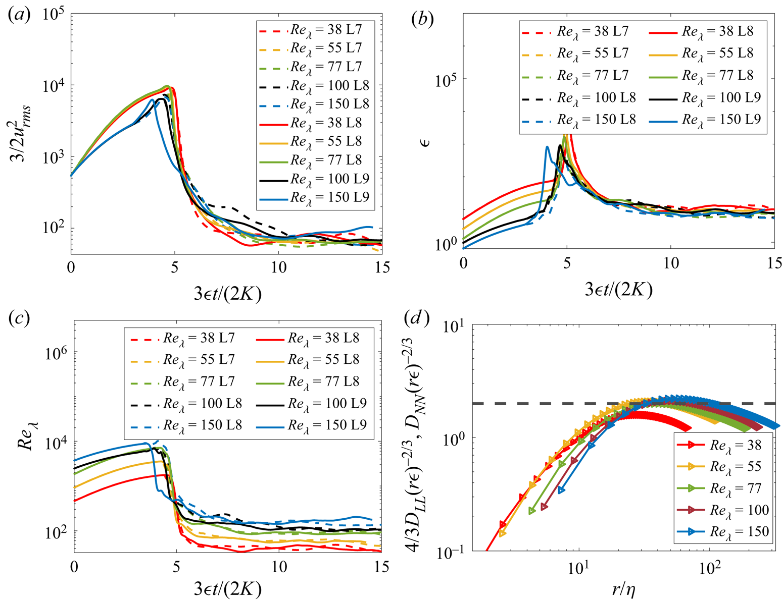
Figure 5. Precursor simulation demonstrating the HIT flow. (a) Kinetic energy as a function of time. (b) Turbulence dissipation rate as a function of time. (c) Reynolds number at the Taylor length scale as a function of time. In all cases, these quantities reach a statistically stationary value after some time, and the bubble is inserted in this HIT flow. (d) Second-order structure function, which demonstrates good agreement with turbulence scaling.
4.2. Bubble insertion
A bubble is inserted at the centroid of the cubic domain that has achieved a stationary HIT state, i.e. for  $t_0 > 15t_c$. The bubble has diameter $d_0$, viscosity $\mu _g$, density $\rho _g$, and surface tension coefficient $\gamma$. The Weber number ${We} = 2\rho _{l}\epsilon ^{2/3}d_0^{5/3}/\gamma \approx 2$ is kept below the critical value for break-up, ${We}_c$ (Rivière et al. Reference Rivière, Mostert, Perrard and Deike2021) so that the bubble might deform but never breaks. With bubble dissolution, the bubble's diameter, and hence the Weber number, reduce further, so that we never observe bubble break-up. Note that the forcing of the turbulence continues to be applied as in Perrard et al. (Reference Perrard, Rivière, Mostert and Deike2021), Rivière et al. (Reference Rivière, Mostert, Perrard and Deike2021) and Farsoiya et al. (Reference Farsoiya, Popinet and Deike2021) once the bubble is inserted, and that we do not consider the effects of gravity/buyoancy.
The bubble has initial gas concentration  $c = \rho _g/M_w$, with the solubility and diffusivity of the gas in the outside fluid given by $\alpha$ and $\mathscr {D}_l$, respectively. The turbulence properties and simulation parameters are given in table 1. The highest resolutions for ${Sc} = 1$ and ${Sc} = 10,30$ cases are L10 and L12, respectively. Figure 6 shows a 3-D rendering of the concentration field for ${Re}_\lambda = 150$, ${Sc}=10$, for the time of bubble insertion (figure 6a) and then three instants during the first eddy turnover time. The bubble size can be seen as being reduced while the gas diffuses out, following turbulent fluctuations. The vorticity field is also indicated.
Table 1. Parameters (with adaptive mesh refinement) of the simulations of bubble dissolution in turbulence. Four Reynolds numbers are used, while the Weber number (below break-up threshold), density and viscosity ratio are kept constant. The solubility  $\alpha = 0.3$ is for cases with ${Sc} = 1$ only.
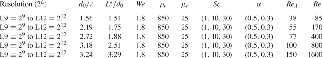

Figure 6. Concentration field for  ${Re}_\lambda =150$, ${Sc} = 10$ at (a) $t = t_0$ (bubble insertion), (b) $(t-t_0)/t_c=0.5$, (c) $(t-t_0)/t_c=0.75$, and (d) $(t-t_0)/t_c=1$. Diffusion of gas around the bubble is shown by field $c$: the darker blue region is a high concentration inside the bubble, and yellow is a low concentration distributed due to advection and diffusion. Magnitude of vorticity is shown at the boundaries of the box behind the bubble.
Another illustration of the dissolution dynamics in turbulence is provided in figure 7. Figures 7(a–d) show the reduction in bubble volume at different time instants for the case  ${Re}_\lambda = 150$, ${Sc}=1$. Note that the bubble volume reduces at a faster rate compared to the radius. The interface shown at $(t-t_0)/t_c = 2.5$ corresponding to $R(t)/R(0) \approx 0.4$ implies $V(t)/V(0) \approx 0.064$. The bubble interface is shown at an instant $(t-t_0)/t_c=1$ in figures 7(e–h), for two $Sc$ values (1 and 10), for the same turbulence condition. The vorticity field on a plane intersecting the bubble is shown in figures 7(e, f) and the corresponding concentration field is shown in figures 7(g,h) for ${Sc} = 1$ and ${Sc} = 10$, respectively. In figure 7(h), the transient boundary layers for ${Sc} = 10$ are thinner compared to ${Sc} = 1$ (figure 7g). The smaller bubble size can also be noticed in figure 7(g) ( ${Sc} = 1$) compared to figure 7(h) ( ${Sc} = 10$), as more mass has diffused into the outer fluid. The concentration fields are similar to the patterns of the surrounding vorticity field.

Figure 7. Interface of bubble at different time instants showing dissolution for the case  ${Re}_\lambda = 150$, ${Sc}=1$, with vorticity field shown on a planar slice at the boundary behind the bubble: (a) $(t-t_0)/t_c = 0$, (b) $(t-t_0)/t_c = 1$, (c) $(t-t_0)/t_c = 2$, and (d) $(t-t_0)/t_c = 2.5$. Vorticity and concentration field (shown on a planar slice intersecting the bubble) for ${Re}_\lambda =150$ at $(t-t_0)/t_c=1$ for (e,g) ${Sc} = 1$, ( f,h) ${Sc} = 10$.
4.3. Dynamics and mass transfer associated with bubble dissolution in turbulence
The time evolution of the bubble radius and associated non-dimensional mass transfer coefficient are shown in figure 8 for increasing Reynolds number ( ${Re}_\lambda = 38$, ${Sc}=1$, $\alpha = 0.5,0.3$ in figures 8(a,b), ${Re}_\lambda = 55$, ${Sc}=10$, $\alpha = 0.5$ in figures 8(c,d), and ${Re}_\lambda = 150$, ${Sc}=10$, $\alpha = 0.5$ in figures 8(e, f)). The mass transfer coefficient $k_L$ is calculated using (3.3b), and the associated instantaneous ${Sh}(t)$ is defined as ${Sh}(t)=k_L(t) L^\star /\mathscr {D}_l$. The mass boundary layer thickness $\delta _k \approx d_0 \,{Pe}^{1/2}$ is resolved up to 4 cells for each case by increasing the resolution.

Figure 8. Bubble size and non-dimensional mass transfer coefficient (based on the initial bubble size), as a function of time: (a,b)  ${Re}_\lambda = 38$, ${Sc}=1$; (c,d) ${Re}_\lambda = 55$, ${Sc}=10$; (e, f) ${Re}_\lambda = 150$, ${Sc}=10$. The ${{Sc} = 1}$ results are converged between L9 and L10, and the ${Sc}=10$ results are converged between L10 and L12. Solubility $\alpha$ rescales the constant concentration at the bubble boundary, $k_L = ({\rm d} c/{\rm d} t)/(\alpha c_g)$.
Figure 8(a) shows that the time evolution of the bubble radius is grid-converged between L9 and L10 for  $Sc=1$. Next, figure 8(b) shows that the non-dimensional transfer coefficient is almost constant with time, and ${Sh}(t)$ (non-dimensionalized $k_L$) reaches a stationary value, while the bubble size is shrinking. The results at ${Re}_\lambda = 55$, ${Sc}=10$ confirm this observation, as shown in figures 8(c,d), with convergence obtained between L10 and L11. For ${Re}_\lambda = 150$, ${Sc}=10$, the time evolution of the bubble radius and ${Sh}$ is converging to a constant value as resolution is increased to L12. The features in figure 8 are general to all the cases that we simulated for a wide range of $Re$ and $Sc$, as summarized in table 1.
We also test the sensitivity of the transfer rate results with the Stefan number, or gas solubility. The Stefan number is  ${St} = \alpha /(1-\alpha ) = 1$ for $\alpha = 0.5$, and ${St} \approx 0.43$ for $\alpha = 0.3$. The effect of solubility $\alpha$ and concentration of the bubble should not affect the mass transfer coefficient $k_L$ for fully unsaturated $c_l=0$ conditions as it just rescales the constant concentration at the bubble boundary $k_L = ({\rm d} c/{\rm d} t)/(\alpha c_g - c_l)$. This can also be seen in figure 8(b), where there is negligible change in $k_L$ when $\alpha$ is reduced from 0.5 to 0.3. As the Reynolds and Schmidt numbers are increased, the boundary layer thickness decreases as $\delta _k \sim {Pe}^{-1/2}$.
The observation of a constant mass transfer coefficient while the bubble size is shrinking contradicts the proposed scaling from Levich (Reference Levich1962) for the mass transfer coefficient in turbulence,  ${Sh} \propto (d/L^\star )\,{Re}^{3/4}\,{Sc}^{1/2}$, which involves a bubble size dependence $d$, as well as our more recent scaling ${Sh}/{Sc}^{1/2} \propto {Re}^{1/2}$ (Farsoiya et al. Reference Farsoiya, Popinet and Deike2021). As the bubble size was constant in Farsoiya et al. (Reference Farsoiya, Popinet and Deike2021), the dependency with bubble size had not been tested. We performed additional simulations with the dilute transfer framework from Farsoiya et al. (Reference Farsoiya, Popinet and Deike2021), varying the bubble sizes in the same turbulent flow and confirm that the mass transfer coefficient $k_L$ in turbulence does not depend on the bubble size, as demonstrated in figure 8. This result can be rationalized by the fact that the smallest length scale of the turbulent flow will control the gas exchange, as described by Lamont & Scott (Reference Lamont and Scott1970) and the high $Re$ regime from Theofanous et al. (Reference Theofanous, Houze and Brumfield1976). As will be shown in the next subsection, all the data from the present study and Farsoiya et al. (Reference Farsoiya, Popinet and Deike2021) can be described by a high $Re$ scaling reading, ${Sh}/{Sc}^{1/2} \propto {Re}^{3/4}$, with the Reynolds number and the Sherwood number defined using the integral length scale $L^\star$: ${Sh}=k_L L^*/\mathscr {D}_l$ and ${Re} = u_{rms}L^\star /\nu _l$, with $u_{rms}$ the velocity fluctuations.
Figure 9(a) shows the concentration of gas transferred in the liquid as a function of time for  ${Re} = 38$, ${Sc} = 1$. The mass transfer rate ${\rm d} N/{\rm d} t \propto -k_L A$ reduces as the bubble size decreases, and reaches zero when the bubble gets dissolved completely as $A \rightarrow 0$ (figure 9a). The corresponding rate of change of the bubble volume is then ${\rm d} V/{\rm d} t \propto {\rm d} N/{\rm d} t \propto -k_L A$. For a spherical bubble, $V\propto R(t)^3$, $A\propto R(t)^2$, so we have ${\rm d}(R(t)^3)/{\rm d} t \propto -k_L\,R(t)^2$, and this implies ${\rm d} R/{\rm d} t \propto -k_L\ (\textrm {or}\ Sh)$. Figure 9(b) shows the normalized rate of change of the bubble radius as a function of the Sherwood number, and we indeed observe $({\rm d} R/{\rm d} t) L^*/(\alpha \mathscr {D}_l)\propto {Sh}$. (The data in figure 9(b) have Pearson correlation coefficient $\rho (({\rm d} R/{\rm d} t) L^*/(\alpha \mathscr {D}_l),{Sh}) = 0.94$.) As discussed above, the transfer rate $k_L$ and its non-dimensional version ${Sh}$ are constant while the bubble dissolves (see figures 8b,d), so the rate of change of the bubble radius is approximately linear with time (which is visible in figures 8a,c). Even if the mass transfer coefficient $k_L$ is independent of the bubble size, a larger bubble has a larger interfacial area, leading to a higher mass transfer than a smaller one. The interfacial area is the determining factor for a given $k_L$, and if a larger bubble breaks into smaller bubbles due to the turbulence, then more surface area is created and the gas transfer increases.
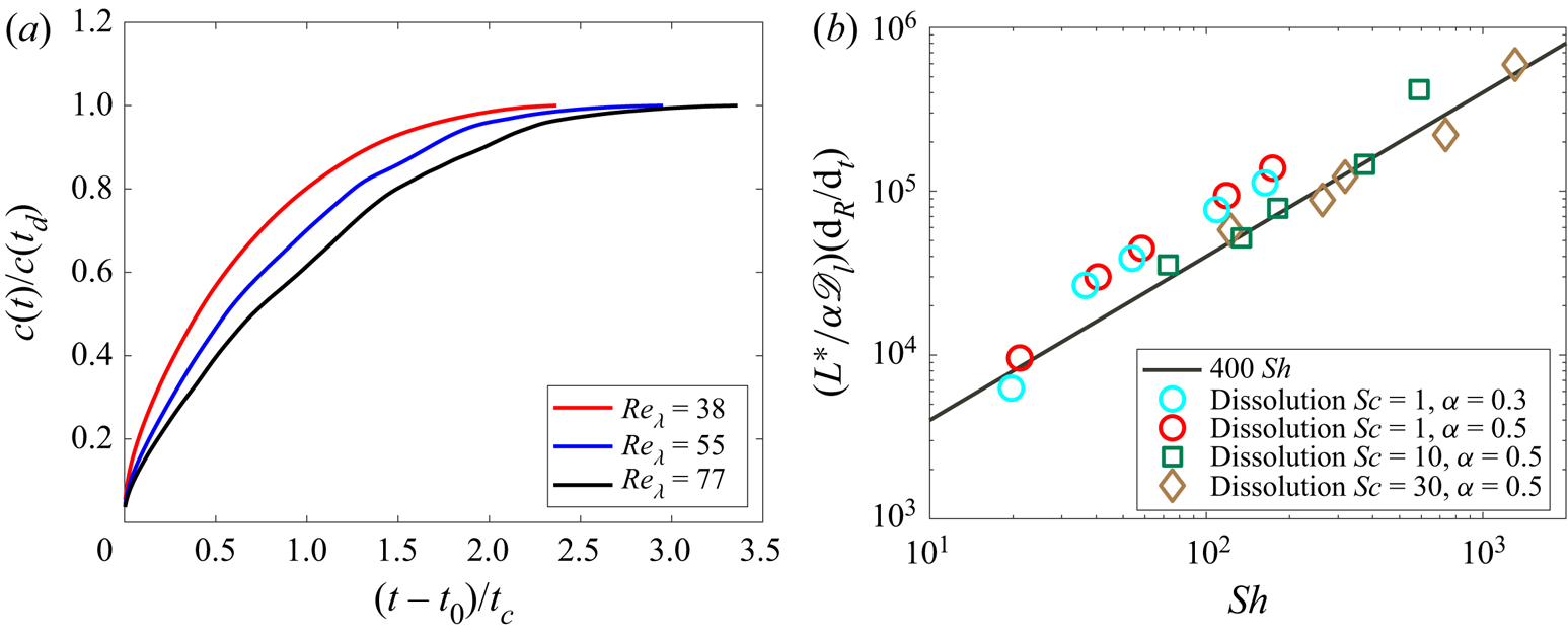
Figure 9. (a) Normalized concentration of gas in surrounding liquid (where  $c(t_d)$ is the gas concentration in the liquid when the bubble is dissolved completely) for case ${Sc}=1$ (highest resolution, L10) for increasing Reynolds number. The gas transfer rate ${\rm d} c/{\rm d} t$ decreases and reaches zero as the bubble dissolves fully. (b) Normalized rate of change of the bubble radius $({\rm d} R/{\rm d} t) L^*/(\alpha \mathscr {D}_l)$ as a function of $Sh$ (highest resolution points). A linear scaling is observed.
4.4. Model for the mass transfer coefficient
The mass transfer coefficient  $k_L$ from the classic penetration theory (Higbie Reference Higbie1935) reads
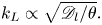 \begin{equation} k_L \propto \sqrt{{\mathscr{D}_l}/{\theta}}. \end{equation}
We observe that the mass transfer coefficient is a function of the bulk turbulence characteristics, but not the bubble size, so we propose the time factor  $\theta$ for the gas diffusion in an HIT flow to scale with the Kolmogorov time scale $\tau _\eta = (\nu _l/\epsilon )^{1/2}$ or integral time scale $\tau _{L^\star } = L^\star /u_{rms}$. A similar discussion for scalings of the exchange velocities can be found in Lamont & Scott (Reference Lamont and Scott1970), Theofanous et al. (Reference Theofanous, Houze and Brumfield1976) and Herlina & Wissink (Reference Herlina and Wissink2016).
Considering the Kolmogorov time scale, the mass transfer coefficient scales as
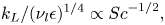 \begin{equation} {k_L}/{(\nu_l \epsilon)^{1/4}} \propto {Sc}^{{-}1/2}, \end{equation}
while considering the integral time scale, the coefficient scales as
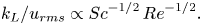 \begin{equation} k_L/u_{rms} \propto {Sc}^{{-}1/2}\,{Re}^{{-}1/2}. \end{equation}
 If we scale  $k_L$ by $\mathscr {D}_l/L^\star$, and define a turbulent Sherwood number ${Sh}=k_L L^*/\mathscr {D}_l$, then we obtain
 \begin{equation} {Sh}/{{Sc}^{1/2}} \propto {Re}^{3/4} \end{equation}
and
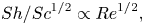 \begin{equation} {Sh}/{{Sc}^{1/2}} \propto {Re}^{1/2}, \end{equation}
respectively. The scaling equation (4.5) would be expected to apply only at a high enough Reynolds number while (4.6) would apply to a lower  $Re$, similarly to the discussion in Theofanous et al. (Reference Theofanous, Houze and Brumfield1976).
Figure 10 shows the turbulent Sherwood number  ${Sh}$ for all the simulations for the cases given in table 1 at the highest numerical resolution (convergence of $Sh$ when resolution is increased is discussed in Appendix A). The error bars depict the minimum and maximum values of $Sh$ after reaching stationary state and before the end of the simulation. All cases with ${Sc}=1$ for all Reynolds numbers (from table 1) are converged to the scaling ${Sh}/{Sc}^{1/2} \propto {Re}^{3/4}$. The ${Sc}=10$ cases are converged to the scaling for ${Re} \leq 400$, as the resolution is increased from L10 to L11, while at the highest $Sc$, the L12 resolution cases are converging. The accepted resolution criteria for direct numerical simulations in the literature (Overholt & Pope Reference Overholt and Pope1996; Pope Reference Pope2001; Schumacher, Sreenivasan & Yeung Reference Schumacher, Sreenivasan and Yeung2005; Dodd et al. Reference Dodd, Mohaddes, Ferrante and Ihme2021; Farsoiya et al. Reference Farsoiya, Popinet and Deike2021) are typically $k_{max}\eta > 1.5$ and $k_{max}\eta _B > 1.5$, where $k_{max}$, $\eta$ and $\eta _B$ are the maximum resolved wavenumber $k_{max}={\rm \pi} N/L$, and the Kolmogorov and Batchelor scales, respectively. The Kolmogorov length scale $\eta =(\nu _l^3/\epsilon )^{1/4}$ defines the length scale at which viscous dissipation becomes dominant, while the Batchelor scale is defined as $\eta _B=\eta /\sqrt {Sc}$. In all of the cases, the Kolmogorov length scale is well resolved, with $k_{max}\eta > 8$, in agreement with the fact that convergence is already achieved in lower resolutions, as shown in figure 5(a). For the highest Péclet number ${Pe} = 4.8 \times 10^4$ ( ${Re} = 1600$, ${Sc}=30$), the Batchelor length scale is resolved up to $k_{max}\eta _B \approx 4$ (refinement $d_0/{\rm \Delta} x = 546$). The boundary layer thickness is $\delta _{\nu } \gtrapprox 2 \eta$ and $\delta _{k} \gtrapprox 2 \eta _B$.
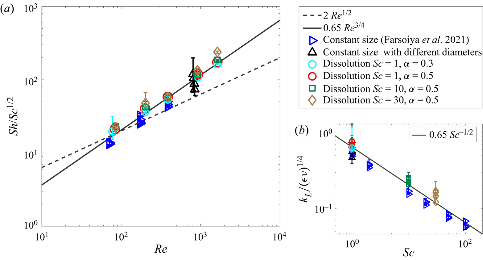
Figure 10. (a) Mean non-dimensional mass transfer coefficient  ${Sh}$ after reaching stationary state and $R(t)>0.3R_0$, normalized by ${Sc}^{1/2}$. The highest (converged) resolution points are shown from table 1. Lines provide the power law for ${Re}^n$, where ${Re} = L^\star u_{rms}/\nu _l$, with a solid line for $n=3/4$, and a dashed line for $n=1/2$. The high $Re$ data align with the $n=3/4$ exponent (when grid convergence is achieved). Circles, squares and diamonds are dissolving data, while triangles are simulations performed under the dilute approximation; see Farsoiya et al. (Reference Farsoiya, Popinet and Deike2021). All data converge to ${Sh}/{Sc}^{1/2} \propto {Re}^{3/4}$. (b) The same scaling but with data plotted as $k_L/(\epsilon \nu )^{1/4}$ as a function of $Sc$, leading to $k_L/(\epsilon \nu )^{1/4}\propto {Sc}^{-1/2}$ (solid line).
The data from dilute gas transfer where bubble size is constant from Farsoiya et al. (Reference Farsoiya, Popinet and Deike2021) also show agreement with (4.5) within narrow error bounds. A new set of simulations for a constant size bubble (Farsoiya et al. Reference Farsoiya, Popinet and Deike2021) with different diameters ( $d_0/\eta \approx 33,17,8,4$) is shown by upward triangles at ${Re}=800$ in figure 10. This also corroborates that the mass transfer coefficient $k_L$ (or $Sh$) is independent of the bubble size. We note that the constant size dilute mass transfer study used a different numerical method (Farsoiya et al. Reference Farsoiya, Popinet and Deike2021) and typically higher resolution. At the same resolutions, the error bars between the two methods are comparable. In summary, at the highest resolution and when the Bachelor length scale is resolved, we observe that the transfer coefficient follows the high $Re$ scaling, (4.5) and ${Sh}/Sc^{1/2}\propto {Re}^{3/4}$, so that the smallest scales of the turbulent flow drive the mass transfer from the bubble.
The mass transfer scaling can be expressed in terms of  $k_L/(\epsilon \nu _l)^{1/4}\propto {Sc}^{-1/2}$ and is shown in figure 10(b). A similar conclusion can be made, with convergence to (4.3) at a high enough grid resolution. We note that a higher $Sc$ is achieved for the dilute case and confirms the above discussion.
5. Conclusion
We developed a numerical framework to simulate gas transfer across fluid–fluid interfaces including volume change effects. The numerical framework is tested against theoretical and numerical solutions of moving boundary problems. For a bubble rising in a quiescent liquid, the mass transfer coefficient  $k_L$ can be described by $k_L = (2/\sqrt {{\rm \pi} })\sqrt {\mathscr {D}_l\,U(t)/d(t)}$, with $d(t)$ and $U(t)$ the time-varying bubble size and rise velocity. For a bubble in a homogeneous and isotropic turbulence flow, with size initially within the inertial range, we found that the mass transfer coefficient for varying bubble size and Reynolds number is independent of the bubble size. The results are obtained using two types of numerical methods: the one from the present study, which allows for dissolution, and the one presented by Farsoiya et al. (Reference Farsoiya, Popinet and Deike2021) under the dilute approximation, provided that the turbulent microscales and boundary layers are resolved at least up to 4 grid points. The transfer rate in the turbulent flow is controlled by the smallest scale in the flow and can then be described as a function of the Reynolds number and Schmidt number by the scaling ${Sh}/{Sc}^{1/2} \propto {Re}^{3/4}$, where ${Sh}=k_L L^\star /\mathscr {D}_l$ is a turbulence Sherwood number. This scaling is equivalent to ${k_L}\propto {Sc}^{-1/2} (\epsilon \nu _l)^{1/4}$, in agreement with the model proposed by Lamont & Scott (Reference Lamont and Scott1970) and corresponding to the high $Re$ regime from Theofanous et al. (Reference Theofanous, Houze and Brumfield1976). This improved understanding of bubble-mediated gas transfer could be applied to complex systems such as gas transfer related to breaking waves at the air–sea interface or gas transfer in bubble swarms.
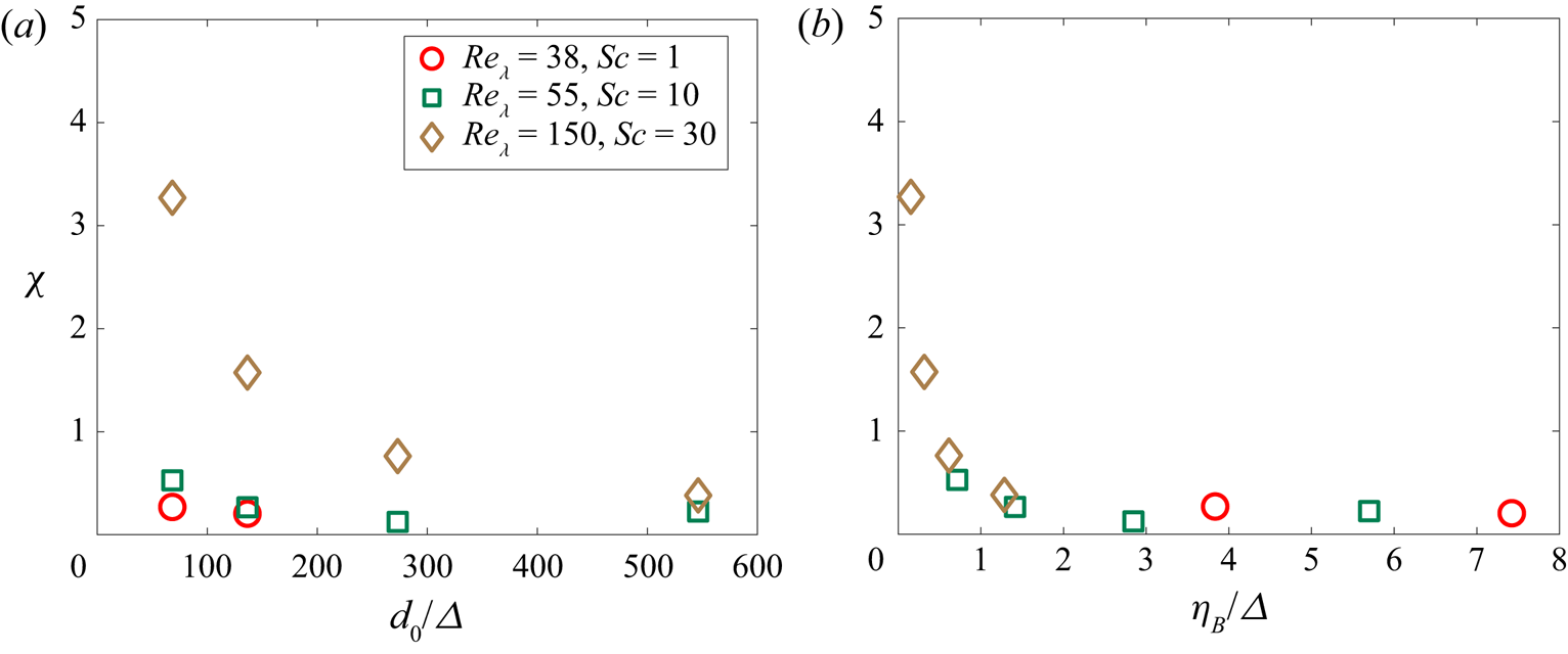
Figure 11. Difference between theoretical scaling and numerical data as a function of the grid resolution (level). This is similar to an error convergence plot. We consider  $\chi = |{Sh} - 0.65\, {Re}^{3/4}\, {Sc}^{1/2}|/(0.65 \, {Re}^{3/4}\,{Sc}^{1/2})$ for some cases in table 1. The error decreases with increased resolution, converging towards the theoretical scaling. (a) Number of grid cells per initial diameter of the bubble. (b) Number of grid cells per Batchelor scale.
Table 2. Numerical values for  ${Sh}/{Sc}^{1/2}$.

Funding
This work was supported by the NSF award 2122042 to L.D., the Catalysis Initiative at Princeton, and the Cooperative Institute for Modeling the Earth System (CIMES) between Princeton and NOAA-GFDL. We would like to acknowledge high-performance computing support from the Extreme Science and Engineering Discovery Environment (XSEDE) (Towns et al. Reference Towns2014), which is supported by the NSF using allocation TG-OCE180010 to L.D. and Cheyenne (doi:10.5065/D6RX99HX) provided by NCAR's Computational and Information Systems Laboratory sponsored by the NSF.
Declaration of interests
The authors report no conflict of interest.
Appendix A. Grid convergence of the mass transfer rate
Figure 11 shows the normalized difference between the numerical mass transfer coefficient and the theoretical scaling proposed (see (4.5)):
 \begin{equation} \chi = |{Sh} - 0.65 \,{Re}^{3/4}\,{Sc}^{1/2}|/(0.65 \, {Re}^{3/4}\,{Sc}^{1/2}) \end{equation}
for increasing grid resolutions. The values are  $\chi \leq 0.5$ and decreasing when going to L11. For higher Péclet numbers, more refined grids are used and allow us to bring the values of $\chi$ below 0.5. Note that the parameter $\chi$ used here is for grid convergence, calculated based on a proportionality constant in (4.5) for best fit in figure 10, and is within $O(1)$ for the data plotted on a log-log scale. Table 2 shows the values for the data points presented in figure 10.
Appendix B. Computational cost
The computational cost for the present study is given in table 3.
Table 3. Computational cost (with adaptive mesh refinement) of the simulations of bubble dissolution in turbulence.


 Open access