


1. Introduction
The rheology of plate-like particles is of interest in many industrial and environmental applications, such as the transport of clay particles in rivers (Tawari, Koch & Cohen Reference Tawari, Koch and Cohen2001), the dispersion of two-dimensional (2-D) nanomaterials in liquid-based composites (Kumar, Sharma & Dixit Reference Kumar, Sharma and Dixit2019) and the development of new-generation lubricants (He et al. Reference He, Xiao, Choi, Díaz, Mosby, Clearfield and Liang2014a,Reference He, Xiao, Kyle, Terrell and Liangb; Xiao & Liu Reference Xiao and Liu2017; Xiao et al. Reference Xiao, Liu, Xu and Zhang2019; Shah et al. Reference Shah, Shahabuddin, Sabri, Salleh, Said and Khedher2021). As for rod-like particles, shape anisotropy in plate-like particle suspensions induces preferred orientations in flow. The change in orientational microstructure affects both the rheological response of the suspension and the occurrence of flow instabilities (Gillissen & Wilson Reference Gillissen and Wilson2018; Gillissen et al. Reference Gillissen, Cagney, Lacassagne, Papadopoulou, Balabani and Wilson2020; Assen et al. Reference Assen, Ng, Will, Stevens, Lohse and Verzicco2022).
At high rotational Péclet numbers, a no-slip plate-like particle suspended in a simple shear flow tumbles, rotating with the same sense of rotation as the undisturbed vorticity vector. While rotating, each particle spends most of the time aligned in the flow direction (Jeffery Reference Jeffery1922), so that, in a time-average or ensemble-average sense, the average orientation of the particle is in the flow direction. In the opposite limit of zero Péclet number, Brownian noise induces a random particle orientation. The average particle orientation angle, and its dependence on the Péclet number  $Pe$, directly affect the macroscopic properties of the suspension, such as the effective viscosity $\eta ^{{eff}}$ (Leal & Hinch Reference Leal and Hinch1971; Hinch & Leal Reference Hinch and Leal1972; Okagawa, Cox & Mason Reference Okagawa, Cox and Mason1973; Rallison Reference Rallison1978; Yamamoto & Matsuoka Reference Yamamoto and Matsuoka1997; Pozrikidis Reference Pozrikidis2001, Reference Pozrikidis2005; Meng & Higdon Reference Meng and Higdon2008; Guo, Zhou & Wong Reference Guo, Zhou and Wong2021) and the average normal stress difference (Okagawa et al. Reference Okagawa, Cox and Mason1973; Rallison Reference Rallison1978). For example, because of the change in average orientation angle with $Pe$, a dilute suspension of plate-like particles shows a shear-thinning behaviour as $Pe$ increases. Changing the thickness of the particle alters both $\eta ^{{eff}}$ and the average normal stress difference. In particular, for dilute suspensions of no-slip particles at concentration $c\to 0$ and fixed $Pe$ suspended in a fluid of viscosity $\eta$, the intrinsic viscosity $\sigma _{xy}'=(\eta ^{{eff}}-\eta )/\eta c$ is predicted to increase as the thickness-to-length particle aspect ratio $k$ decreases (Leal & Hinch Reference Leal and Hinch1971; Hinch & Leal Reference Hinch and Leal1972; Singh et al. Reference Singh, Koch, Subramanian and Stroock2014).
Two-dimensional nanomaterials such as graphene, Molybdenum disulfide (MoS $_{2}$) and boron nitride can display considerable surface hydrodynamic slip (Kamal, Gravelle & Botto Reference Kamal, Gravelle and Botto2021b), i.e. the fluid does not completely ‘stick’ to the solid as assumed in the no-slip condition. Conditions for a molecularly smooth surface to display large hydrodynamic slip are discussed, for example, in Tocci, Joly & Michaelides (Reference Tocci, Joly and Michaelides2014) and Voeltzel et al. (Reference Voeltzel, Fillot, Vergne and Joly2018). The slip lengths, typically a few tens of nanometres, are small compared with microscopic scales but are still much larger than the thickness of 2-D nanomaterial particles. What is the effect of hydrodynamic slip on the rheological properties of a dilute suspension of plate-like particles?
We have recently shown through molecular dynamics and continuum simulations that surface slip can cause plate-like particles (platelets) to align indefinitely near the flow direction at high  $Pe$ (Kamal, Gravelle & Botto Reference Kamal, Gravelle and Botto2020; Gravelle, Kamal & Botto Reference Gravelle, Kamal and Botto2021; Kamal et al. Reference Kamal, Gravelle and Botto2021b; Crowdy Reference Crowdy2022). The stable alignment occurs due to surface slip reducing the hydrodynamic traction over the slender surface of the platelet when the platelet is oriented in the flow direction and is in stark contrast to the tumbling motion observed for no-slip platelets.
This article aims to investigate theoretically and numerically the effect of surface slip on the intrinsic viscosity and normal stress difference of a dilute 2-D suspension of plate-like particles suspended in an unbounded shear flow field in the creeping flow limit. In the dilute limit, the intrinsic viscosity  $\sigma '_{xy}$ is well approximated by evaluating the contribution from an isolated particle. The effect of surface slip on $\sigma '_{xy}$ in the case of a dilute suspension of particles has been studied in both the continuum limit for spherical and prolate and oblate ellipsoidal particles (Allison Reference Allison1999; Luo & Pozrikidis Reference Luo and Pozrikidis2007, Reference Luo and Pozrikidis2008), and at the atomic scale through molecular dynamics simulations of plate-like molecules/particles (Gravelle et al. Reference Gravelle, Kamal and Botto2021). These studies observed a reduction in $\sigma '_{xy}$ compared with no-slip particles of identical shape. For example, Allison compared $\sigma '_{xy}$ for isolated perfect-slip and no-slip ellipsoidal particles for $Pe\to 0$ (Allison Reference Allison1999). Allison found that, for an oblate ellipsoid, the flatter the ellipsoid, the greater the reduction in $\sigma '_{xy}$ compared with a no-slip ellipsoid of identical shape, figure 1. The minimum reduction in $\sigma '_{xy}$ between a perfect-slip and no-slip ellipsoidal particle occurs for a sphere. Assuming a Navier slip surface, this reduction in $\sigma _{xy}'$ can be calculated analytically (Luo & Pozrikidis Reference Luo and Pozrikidis2008). A decrease by a factor of $2/5$ in $\sigma _{xy}'$ for an isolated perfect-slip spheroid compared with a no-slip spheroid is found (Luo & Pozrikidis Reference Luo and Pozrikidis2008). In a previous study (Gravelle et al. Reference Gravelle, Kamal and Botto2021) we explored the effect of surface slip on plate-like particles through molecular dynamics simulations for a range of $Pe$. Owing to the relatively large thickness-to-length aspect ratio $k$ of the plate-like molecule ( $k\approx 0.33$), the change in $\sigma '_{xy}$ as $Pe$ increased was found to be small. However, a significant change in $\sigma '_{xy}$ was observed compared with no-slip molecules of equivalent shape.
Intrinsic viscosity vs the inverse of the particle thickness-to-length aspect ratio  $k$ for $Pe\to 0$, comparing oblate ellipsoids with perfect slip or no-slip surfaces (black squares, from Allison Reference Allison1999) and molecular dynamics data for a dilute suspension of disk-shaped nanoplatelets for $Pe=1.0$ (blue circles, from Gravelle et al. Reference Gravelle, Kamal and Botto2021).

Whilst these studies show a significant effect of surface slip on  $\sigma '_{xy}$, the effect of surface slip on the macroscopic properties of suspensions containing ultra-thin platelets remains to be analysed. This article investigates this effect theoretically and numerically for model 2-D slip platelets suspended in a 2-D flow and featuring a Navier slip boundary condition at their surfaces. More specifically, we shall focus on calculating $\sigma '_{xy}$ and the average normal stress difference of the suspension, $\left \langle N\right \rangle$. Our methodology for calculating $\sigma '_{xy}$ and $\left \langle N\right \rangle$ is based on using the boundary integral method (BIM) and its mathematical formulation. The BIM is used to calculate the surface traction over a particle under the continuum Stokes flow assumptions. The advantage of a BIM formulation is that its surface integral formulation can be asymptotically expanded for small $k$ (Singh et al. Reference Singh, Koch, Subramanian and Stroock2014; Kamal et al. Reference Kamal, Gravelle and Botto2020), allowing one to develop simplified equations for the hydrodynamic traction acting on the particle's surface. Therefore, the hydrodynamic traction on platelets with aspect ratios similar to 2-D nanomaterials can be calculated to high accuracy numerically and, in some cases, analytically.
The outline of the article is as follows. In § 1, we describe the set-up of our problem and the BIM formulation governing the traction distribution. The numerical scheme for solving the boundary integral equations is also given. In § 2, we provide an asymptotic analysis of the boundary integral equations. Finally, in § 4, we use our numerical and analytical results to calculate  $\sigma '_{xy}$ and $\left \langle N\right \rangle$ for a dilute suspension of 2-D slip particles and examine their dependence on the slip length, aspect ratio and $Pe$.
$Pe$.
2. Stresslet, viscosity and normal stress difference for a 2-D platelet
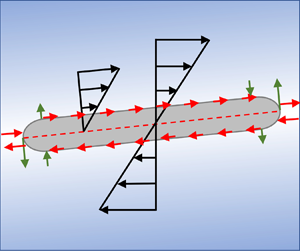
We consider a platelet free to rotate in an external linear shear flow field. In a coordinate system  $(x,y)$, with $x$ along the flow direction and $y$ along the flow gradient direction, the undisturbed flow field is $\boldsymbol {u}^{\infty }=\dot {\gamma }y\boldsymbol {\hat {e}}_{x}$, where $\boldsymbol {\hat {e}}_{x}$ is the unit vector along $x$ (left-hand side sketch in figure 2). We assume that the platelet has an infinite extent in the vorticity direction, so that the problem is effectively two-dimensional, and the cross-section of the body rotates in the $\boldsymbol {\hat {e}}_{x},\boldsymbol {\hat {e}}_y$ plane. We assume that the platelet's cross-section is symmetric about two orthogonal lines passing through its geometric centre. The angle from $\boldsymbol {\hat {e}}_{x}$ to the line of symmetry along the major axis of the particle is $\phi$. The size of the platelet is characterised by its half-length $a$ and half-thickness $b$. We assume that the geometric aspect ratio $k=b/a\ll 1$. Furthermore, we assume the fluid satisfies the linear Navier slip boundary condition on the platelet's surface. The Navier slip velocity $\boldsymbol {u}^{{sl}}=u_{x}^{{sl}}\boldsymbol {\hat {e}}_{x}+u_{y}^{{sl}}\boldsymbol {\hat {e}}_y$ is expressed in terms of the surface traction $\boldsymbol {f}$ as (Kamal et al. Reference Kamal, Gravelle and Botto2021b)
 \begin{equation} u_{x}^{{sl}}=\frac{\lambda}{\eta} (n_{y}^{2} \,f_x-n_x n_y \,f_y),\quad u_{y}^{{sl}}=\frac{\lambda}{\eta} (n_{x}^{2} \,f_y - n_x n_y \,f_x), \end{equation}
where  $\lambda$ is the Navier slip length, $\boldsymbol {n}=n_x\boldsymbol {\hat {e}}_{x}+ n_y\boldsymbol {\hat {e}}_y$ is the unit surface normal pointing out of the particle and $\eta$ is the viscosity of the fluid.
Sketch of a 2-D platelet in an external shear flow field. For a given orientation  $\phi$, the external flow field can be decomposed into two shear components (acting parallel and perpendicular to the major axis of the particle) and an extensional component.

The velocity field  $\boldsymbol {u}$, the stress tensor field $\boldsymbol {\sigma }$ and the pressure field $p$ are assumed to satisfy the incompressible Stokes equations
 \begin{equation} \boldsymbol{\nabla}\boldsymbol{\cdot} \boldsymbol{\sigma}=0,\quad \boldsymbol{\nabla}\boldsymbol{\cdot}\boldsymbol{u}=0,\quad \sigma_{ij}=-\delta_{ij} p +\eta \left(\frac{\partial {u}_{i}}{\partial x_{j}}+ \frac{\partial {u}_{j}}{\partial x_{i}}\right). \end{equation}
The contribution to the bulk stress from a torque-and-force-free particle can be found by calculating the stresslet tensor (Batchelor Reference Batchelor1970). The stresslet tensor is defined as (Pozrikidis Reference Pozrikidis1992)
 \begin{equation} {\mathsf{S}}_{ij}(\phi)=\tfrac{1}{2}\int_{{\mathcal{L}}} \left[\,f_i(\phi) x_j+f_j(\phi) x_i-\tfrac{2}{3}\delta_{ij}x_k\,f_k(\phi)-2\eta(u^{{sl}}_i n_j + u^{{sl}}_j n_i)\right] \mathrm d{L}, \end{equation}
where  ${x}_i$ is the position vector with respect to the platelet's geometric centre, the integral is over the boundary ${\mathcal {L}}$ of the platelet's cross-section and $\mathrm d{L}$ is a boundary element. When the boundary of the particles satisfies the no-slip boundary condition, the integral involving the slip velocity is zero, and the stresslet depends only on $\boldsymbol {f}$. When the Navier slip boundary condition is instead applied, the slip velocity makes an additional finite contribution to the stresslet tensor. This term, containing the integral of the slip velocity along the particle surface, is the viscous stress associated with the volume-averaged velocity gradient inside the particle (Batchelor Reference Batchelor1970). In general, the stresslet tensor has a hydrodynamic contribution, which depends on the traction produced by a torque-free particle in an external shear flow field (measured in the laboratory frame), and a Brownian contribution, which depends on the traction due to a random rotation of the particle. From here onwards we will use ${\mathsf{S}}^{h}_{ij}$ to denote the hydrodynamic stresslet tensor and ${\mathsf{S}}^{b}_{ij}$ to denote the Brownian stresslet tensor.
The boundary integral formulation provides a closed expression for  $\boldsymbol {f}$. In this formulation, the velocity of the fluid at a point $\boldsymbol {x}_1$ on ${\mathcal {L}}$ is related to $\boldsymbol {f}$ through the following integral equation:
 \begin{align} & \frac{1}{4{\rm \pi}}\int_{{\mathcal{L}}} \boldsymbol{n}(\boldsymbol{x}) \boldsymbol{\cdot}\boldsymbol{\mathsf{K}}(\boldsymbol{x},\boldsymbol{x}_1) \boldsymbol{\cdot} \boldsymbol{u}^{{sl}}(\boldsymbol{x})\,\mathrm d {L}(\boldsymbol{x}) -\frac{1}{4{\rm \pi}\eta}\int_{{\mathcal{L}}} \boldsymbol{\mathsf{G}}(\boldsymbol{x},\boldsymbol{x}_1) \boldsymbol{\cdot} \boldsymbol{f}(\boldsymbol{x})\,\text{d}{L}(\boldsymbol{x}) \nonumber\\ &\quad =\frac{\boldsymbol{u}^{{sl}}(\boldsymbol{x}_1 )}{2}+\boldsymbol{u}^{{rg}}(\boldsymbol{x}_1)- \boldsymbol{u}^{\infty}(\boldsymbol{x}_1 ) , \end{align}
where  $\boldsymbol {u}^{{rg}}=\varOmega \boldsymbol {\hat {e}}_{z}\times \boldsymbol {x}$ is the rigid body motion of a body centred at the origin. Here, $\varOmega$ is the particle angular velocity and $\boldsymbol {\hat {e}}_{z}=\boldsymbol {\hat {e}}_{x}\times \boldsymbol {\hat {e}}_y$.
The first term on the left-hand side of (2.4) is the double-layer potential, and the second term is the single-layer potential (Pozrikidis Reference Pozrikidis1992). It can be shown that the term containing the slip velocity in the definition of the stresslet tensor given in (2.3) originates from the double-layer potential, and the remaining term originates from the single-layer potential (Pozrikidis Reference Pozrikidis1992).
Since the flow is two-dimensional, the tensors  $\boldsymbol{\mathsf{G}}$ and $\boldsymbol{\mathsf{K}}$ in (2.4) are tensors associated with the 2-D Stokeslet and stresslet, respectively (Pozrikidis Reference Pozrikidis1992). We parametrise $\mathcal {L}$ as ${\mathcal {L}}=\{a s\boldsymbol {\hat {e}}_{s}\pm bh(s)\boldsymbol {\hat {e}}_t: -1 \leq s\leq 1 \}$, where $s$ is the non-dimensional arc length running through the particle's major axis, $b h(s)$ is the thickness of the particle and $\boldsymbol {\hat {e}}_{s}$ and $\boldsymbol {\hat {e}}_t$ are unit vectors parallel to the platelet's major and minor axes, respectively, as sketched in figure 2. The non-dimensional thickness of the platelet $h(s)$ has maximum value $h(0)=1$ and satisfies $h(\pm 1)=0$ at the edges. In the manuscript, we will denote vectors in the $(s,t)$ coordinate system with a subscript. For instance, the coordinates of $\boldsymbol {f}$ along $\boldsymbol {\hat {e}}_{s}$ and $\boldsymbol {\hat {e}}_t$ are denoted $f_s$ and $f_t$, respectively. The symbols $\hat {s}$ and $\hat {t}$, as used in figure 2, denote the dimensional coordinates along $\boldsymbol {\hat {e}}_{s}$ and $\boldsymbol {\hat {e}}_t$ i.e. $\hat {s} = as$ and $\hat {t} = at$.
The effective viscosity of a dilute suspension of identical particles can be expressed as (Leal & Hinch Reference Leal and Hinch1971)
 \begin{equation} \eta_{eff}/\eta=1+\sigma_{xy}' c +O(c^2). \end{equation}
Here,  $\sigma _{xy}'$ is the intrinsic shear viscosity, a coefficient related to ${\mathsf{S}}_{xy}^{h}(\phi )$ and ${\mathsf{S}}^{b}_{xy}(\phi )$ (Kim & Karrila Reference Kim and Karrila2013). For a 2-D system, $c$ corresponds to the areal fraction of the solid, and for a 3-D system, $c$ corresponds to the volume fraction. In general $\sigma _{xy}'$ depends on the shape of the particle (Leal & Hinch Reference Leal and Hinch1971), the Péclet number $Pe$ (Hinch & Leal Reference Hinch and Leal1972) and $\lambda$ (Allison Reference Allison1999). The Péclet number describes the ratio $Pe=\dot {\gamma }/D_r$, where $D_r$ is the rotational diffusion coefficient of the particle (Hinch & Leal Reference Hinch and Leal1972; Kamal et al. Reference Kamal, Gravelle and Botto2021b).
For a 2-D particle,  $\sigma ^{'}_{xy}$ is given by
 \begin{equation} \sigma^{'}_{xy}=\frac{\left\langle {\mathsf{S}}_{xy}^{h}+{\mathsf{S}}_{xy}^{b}\right\rangle}{\dot{\gamma}\eta A_p}=A \left\langle1-\cos{4\phi}\right\rangle+B +\frac{C}{Pe}\left\langle\sin{2\phi}\right\rangle. \end{equation}
Here,  $A$,
$A$,  $B$ and $C$ are dimensionless coefficients which depend on $\lambda$ and the particle shape (Rallison Reference Rallison1978) and $A_p$ is the cross-sectional area of the particle. The angled brackets $\left \langle \,\right \rangle$ represent an average over the steady-state orientation distribution function $p(\phi )$. Equation (2.6) can be obtained from the corresponding 3-D stress tensor for an asymmetric particle (see, for example, Batchelor Reference Batchelor1970) by assuming that the particle axis of rotation is always perpendicular to the $\boldsymbol {\hat {e}}_{x}$– $\boldsymbol {\hat {e}}_y$ plane.
In this article, we focus on calculating the coefficients  $A$,
$A$,  $B$ and $C$ in (2.6). The evaluation of $\left \langle 1-\cos {4\phi }\right \rangle$ and $\left \langle \sin {2\phi }\right \rangle$ is described in Kamal et al. (Reference Kamal, Gravelle and Botto2021b), where these quantities were calculated by solving the 1-D Fokker–Plank equation numerically to obtain $p(\phi )$, and using this function to calculate the angular average of $\cos {4\phi }$ and $\sin {2\phi }$.
The average normal stress difference due to the hydrodynamic traction can be calculated from the diagonal components of the stresslet (Okagawa et al. Reference Okagawa, Cox and Mason1973). For a 2-D system, the normal stress difference is
 \begin{equation} \left\langle N\right\rangle=\frac{1}{\dot{\gamma}\eta A_p} \left\langle {\mathsf{S}}_{xx}-{\mathsf{S}}_{yy}\right\rangle=2A\left\langle\sin{4\phi}\right\rangle. \end{equation}
The normal stress difference is a key quantity to characterise the non-Newtonian features of a suspension of particles (Tanner Reference Tanner2000).
2.1. Decomposition of  ${\mathsf{S}}_{ij}$ for arbitrary $\phi$


Owing to the geometric symmetry of the platelet for any given orientation  $\phi$, $\boldsymbol {f}$ and thus ${\mathsf{S}}_{xy}^{h}(\phi )$ can be expressed in terms of the traction at $\phi =0,\ {\rm \pi}/4$ and ${\rm \pi} /2$ (Masoud, Stone & Shelley Reference Masoud, Stone and Shelley2013; Kamal et al. Reference Kamal, Gravelle and Botto2020). The equation for $\boldsymbol {f}$ at these orientations can be simplified by evaluating (2.4) in the particle frame ( $\boldsymbol {\hat {e}}_{s},\boldsymbol {\hat {e}}_t$). In the particle frame, ${\mathcal {L}}$ can be decomposed into an upper curve ${\mathcal {L}}^+ = \{ (as,bh(s)): -1 \leq s \leq 1 \}$ and lower curve ${\mathcal {L}}^- = \{ (as,-bh(s)): -1 \leq s \leq 1 \}$ located symmetrically with respect to the centreline $t=0$. Taking advantage of this symmetry, $\boldsymbol {f},\ \boldsymbol {u}^{\infty }, \boldsymbol {u}^{{sl}}$ and $\boldsymbol {u}^{{rg}}$ can be decomposed into symmetric and anti-symmetric parts with respect to $t=0$. Given a generic vector quantity $\alpha _i$, the anti-symmetric part of $\alpha _i$ is
 \begin{equation} \text{Asym}\{\alpha_i(s,h)\} = \Delta \alpha_i(s,h) = \frac{\alpha_i(s,h) - \alpha_i(s,-h)}{2}, \end{equation}
and the symmetric part of  $\alpha _i$ is
 \begin{equation} \text{Sym}\{\alpha_i(s,h)\} = \bar{\alpha}_i(s,h) = \frac{\alpha_i(s,h) + \alpha_i(s,-h)}{2}. \end{equation}
With this decomposition, the normal and tangential components of (2.4) result in the following four scalar equations.
Symmetric part, normal component:
 \begin{equation} -\frac{1}{4{\rm \pi}\eta}{\mathsf{G}}_{t}[\Delta f_s,\bar{f}_t]+ \frac{1}{4{\rm \pi}}{\mathsf{K}}_{t}[\Delta u^{{sl}}_s,\bar{u}^{{sl}}_t,\lambda] = \frac{\bar{u}^{{sl}}_t}{2}+a\left(\dot{\gamma}\sin^{2}{\phi}+\varOmega(\phi)\right)s_1. \end{equation}
Symmetric part, tangential component:
 \begin{equation} -\frac{1}{4{\rm \pi}\eta}{\mathsf{G}}_s[\,\bar{f}_s,\Delta f_t]+ \frac{1}{4{\rm \pi}}{\mathsf{K}}_{s}[\bar{u}^{{sl}}_s,\Delta u^{{sl}}_t,\lambda]= \frac{\bar{u}^{{sl}}_s}{2}-a\dot{\gamma}s_1\sin{\phi}\cos{\phi}. \end{equation}
Anti-symmetric part, normal component:
 \begin{equation} -\frac{1}{4{\rm \pi}\eta}{\mathsf{G}}_{t}[\,\bar{f}_s,\Delta f_t]+ \frac{1}{4{\rm \pi}}{\mathsf{K}}_{t}[ \bar{u}^{{sl}}_s,\Delta u^{{sl}}_t,\lambda]= \frac{\Delta u^{{sl}}_t}{2}+b\dot{\gamma}h(s_1)\sin{\phi}\cos{\phi}. \end{equation}
Anti-symmetric part, tangential component:
 \begin{equation} -\frac{1}{4{\rm \pi}\eta}{\mathsf{G}}_s[\Delta f_s,\bar{f}_t]+ \frac{1}{4{\rm \pi}}{\mathsf{K}}_{s}[\Delta u^{{sl}}_s,\bar{u}^{{sl}}_t,\lambda]= \frac{\Delta u^{{sl}}_s}{2}-b\left(\dot{\gamma}\cos^{2}{\phi}+\varOmega(\phi)\right)h(s_1). \end{equation}
 Here, we have used the fact that the reference point  $\boldsymbol {x}_1$ on $\mathcal {L}$ in (2.4) is $\boldsymbol {x}_1 =(a s_1,b h(s_1))$. The integrals ${\mathsf{G}}_s$ and ${\mathsf{G}}_{t}$ are defined as
 $$\begin{gather} {\mathsf{G}}_s[\Delta f_s,\bar{f}_t] = \int_{{\mathcal{L}}^+} \left[{\mathsf{G}}_{ss}^- \Delta f_{s}+{\mathsf{G}}_{ts}^+ \bar{f}_t\right] \mathrm d {L}, \end{gather}$$
 $$\begin{gather}{\mathsf{G}}_{t}[\Delta f_s,\bar{f}_t]=\int_{{\mathcal{L}}^+} \left[{\mathsf{G}}_{nn}^+ \bar{f}_t + {\mathsf{G}}_{st}^- \Delta f_{s} \right] \mathrm d {L}, \end{gather}$$
 $$\begin{gather}{\mathsf{G}}_s[\,\bar{f}_s,\Delta{f}_t]=\int_{{\mathcal{L}}^+} \left[{\mathsf{G}}_{ss}^+ \bar{f}_{s} +{\mathsf{G}}_{ts}^- \Delta{f}_t \right] \mathrm d {L}, \end{gather}$$
 $$\begin{gather}{\mathsf{G}}_{t}[\,\bar{f}_s,\Delta{f}_t]=\int_{{\mathcal{L}}^+} \left[{\mathsf{G}}_{tt}^- \Delta f_t + {\mathsf{G}}_{st}^+ \bar{f}_{s} \right] \mathrm d {L}, \end{gather}$$
where
 \begin{equation}
\boldsymbol{\mathsf{G}}^+=\boldsymbol{\mathsf{G}}(s',h') +
\boldsymbol{\mathsf{G}}(s',\hat{h}),\quad
\boldsymbol{\mathsf{G}}^-=\boldsymbol{\mathsf{G}}(s',h') -
\boldsymbol{\mathsf{G}}(s',\hat{h}),
\end{equation}
\begin{equation}
\boldsymbol{\mathsf{G}}^+=\boldsymbol{\mathsf{G}}(s',h') +
\boldsymbol{\mathsf{G}}(s',\hat{h}),\quad
\boldsymbol{\mathsf{G}}^-=\boldsymbol{\mathsf{G}}(s',h') -
\boldsymbol{\mathsf{G}}(s',\hat{h}),
\end{equation}
and  ${s}'=a(s-s_{1})$, ${h}'=b(h(s)-h(s_{1}))$ and $\hat {h}=-b(h(s)+h(s_{1}))$. The integrals ${\mathsf{K}}_{s}$ and ${\mathsf{K}}_{t}$ are defined as
 $$\begin{gather} {\mathsf{K}}_{i}[\Delta u_s,\bar{u}_t,\lambda]=\int_{{\mathcal{L}}^+} \left[ n_s \Delta u_s\left({\mathsf{K}}^-_{itt}-{\mathsf{K}}^-_{iss}\right) +\left(n_t \Delta u_{s}+n_{s}\bar{u}_t\right){\mathsf{K}}^+_{ist}\right] \mathrm d {L}, \end{gather}$$
 $$\begin{gather}{\mathsf{K}}_{i}[\bar{u}_s,\Delta u_t,\lambda]=\int_{{\mathcal{L}}^+}\left[ n_s \bar u_s\left({\mathsf{K}}^+_{itt}-{\mathsf{K}}^+_{iss}\right)+\left(n_t \bar{u}_{s}+n_{s}\Delta{u}_t\right){\mathsf{K}}^-_{ist}\right] \mathrm d {L}, \end{gather}$$
where  $i=\{s,t\}$, $\boldsymbol{\mathsf{K}}^+=\boldsymbol{\mathsf{K}}(s',h')+\boldsymbol{\mathsf{K}}(s',\hat {h})$ and $\boldsymbol{\mathsf{K}}^-=\boldsymbol{\mathsf{K}}(s',h')-\boldsymbol{\mathsf{K}}(s',\hat {h})$. Under this decomposition, for any orientation $\phi$, the flow field acting on the particle in the particle frame can be decomposed into two simple shear flows, $\boldsymbol {u}^{\infty }_{S}=\dot {\gamma }bh\cos ^2{\phi } \boldsymbol {\hat {e}}_{s}$ and $-\dot {\gamma }as\sin ^2{\phi }\boldsymbol {\hat {e}}_t$ (with streamlines parallel and perpendicular to the particle's major axis, respectively), and an extensional component $\boldsymbol {u}^{\infty }_{E}=\dot {\gamma }(as\cos {\phi }\sin {\phi }\boldsymbol {\hat {e}}_{s}-bh\cos {\phi }\sin {\phi }\boldsymbol {\hat {e}}_t)$, as sketched in figure 2. The compressional axis of the extensional flow component is parallel to the major axis of the particle. Equations (2.10) and (2.13) are equations for the hydrodynamic tractions $\Delta f_s$ and $\bar {f}_t$ due to $\boldsymbol {u}^{\infty }_{S}$. Equations (2.12) and (2.11) are equations for $\Delta f_t$ and $\bar {f}_{s}$ due to $\boldsymbol {u}^{\infty }_{E}$. Under this decomposition, for any orientation $\phi$, $\boldsymbol {f}$ can be calculated exactly by solving (2.10) and (2.13) for $\phi =0$ and $\phi ={\rm \pi} /2$, and (2.12) and (2.11) for $\phi = {\rm \pi}/4$. Therefore, to calculate ${\mathsf{S}}_{ij}(\phi )$, one only needs to calculate $\boldsymbol {f}$ at $\phi =0$ and $\phi ={\rm \pi} /2$ for the ‘shear’ components of the flow field and at $\phi ={\rm \pi} /4$ for the ‘extensional’ component.
2.2. Calculation of the stress coefficients
For a force-and-torque-free body, the angular velocity of the platelet satisfies (Bretherton Reference Bretherton1962; Kamal et al. Reference Kamal, Gravelle and Botto2021b)
 \begin{equation} \varOmega(\phi)=-\frac{\dot{\gamma}}{1+k_e^2}(k_e^2\cos^2{\phi}+\sin^{2}{\phi}), \end{equation}
where  $k_e=\sqrt {T(0)/T({\rm \pi} /2)}$ is the square root of the ratio between the torques exerted on a particle held fixed parallel ( $T(0)$) and perpendicular ( $T({\rm \pi} /2)$) to the flow. The torque acting on a particle fixed at an orientation angle $\phi$ is
 \begin{equation} T(\phi)=\boldsymbol{\hat{e}}_{z}\boldsymbol{\cdot}\int_{\mathcal{L}}\boldsymbol{f}\times{\boldsymbol{x}}\,\text{d}L. \end{equation}
 The parameter  $k_e$ is commonly called the ‘effective-aspect ratio’ because, at least for the case of no-slip particles (Singh et al. Reference Singh, Koch, Subramanian and Stroock2014; Abtahi & Elfring Reference Abtahi and Elfring2019), it ‘effectively’ describes the rotational behaviour of an equivalent no-slip axisymmetric ellipsoidal particle with geometric aspect ratio $k=k_e$ (Jeffery Reference Jeffery1922; Bretherton Reference Bretherton1962).
Noting that  $\varOmega (0)=k_e^2\varOmega ({\rm \pi} /2)=-\dot {\gamma }k_e^2/(1+k_e^2)$, we use this expression to simplify (2.10) and (2.13) for $\phi =0$ and $\phi ={\rm \pi} /2$, respectively. Upon simplification, one finds the resulting equations for $\phi = 0$ and $\phi = {\rm \pi}/2$ are identical except for the sign. It follows that the hydrodynamic stresslet tensor evaluated in the particle frame is
 \begin{equation} {\mathsf{S}}_{st}^{h}(0)=-{\mathsf{S}}_{st}^{h}({\rm \pi}/2)=\int_{{\mathcal{L}}^+} \left[b\Delta f_s h+a\bar{f}_ts-2\eta(\Delta u^{{sl}}_s n_t+\bar u^{{sl}}_t n_s) \right]\mathrm d {L}, \end{equation}
where  $\Delta f_s$ and $\bar {f}_t$ are evaluated for $\phi =0$. Also, it follows that ${\mathsf{S}}_{st}^{h}({\rm \pi} /4)={\mathsf{S}}_{st}^{h}(0)\cos {\phi }+{\mathsf{S}}_{st}^{h}({\rm \pi} /2)\sin {\phi }=0$, ${\mathsf{S}}_{ss}^{h}(0)={\mathsf{S}}_{tt}^{h}(0)=0$ and
 \begin{equation} {\mathsf{S}}_{ss}^{h}({\rm \pi}/4)-{\mathsf{S}}_{tt}^{h}({\rm \pi}/4)=2\int_{{\mathcal{L}}^+} \left[a\bar{f}_s s-b\Delta f_t h-2\eta(\bar u^{{sl}}_s n_s-\Delta u^{{sl}}_t n_t )\right]\mathrm d {L}, \end{equation}
where  $\bar {f}_s$ and $\Delta f_t$ are evaluated for $\phi ={\rm \pi} /4$. Hence, the stresslet tensor can be written in the particle frame as
 \begin{equation}
{\mathsf{S}}^{h}_{ij}(\phi)=(\delta_{si}\delta_{tj}+\delta_{ti}\delta_{sj}){\mathsf{S}}^{h}_{st}(0)
(\cos^2{\phi}-\sin^2{\phi})+2\delta_{ij}{\mathsf{S}}^{h}_{ii}({\rm \pi}/4)\cos{\phi}\sin{\phi}.
\end{equation}
\begin{equation}
{\mathsf{S}}^{h}_{ij}(\phi)=(\delta_{si}\delta_{tj}+\delta_{ti}\delta_{sj}){\mathsf{S}}^{h}_{st}(0)
(\cos^2{\phi}-\sin^2{\phi})+2\delta_{ij}{\mathsf{S}}^{h}_{ii}({\rm \pi}/4)\cos{\phi}\sin{\phi}.
\end{equation}
Therefore, one only needs to calculate  $\boldsymbol {f}$ for $\phi =0$ and ${\rm \pi} /4$ to evaluate ${\mathsf{S}}_{ij}^{h}(\phi )$. Transforming ${\mathsf{S}}^{h}_{ij}$ back to the laboratory frame by use of a rotation matrix ${\mathsf{R}}_{ij}(\phi )$, one finds
 \begin{equation}
{\mathsf{S}}^{h}_{xy}(\phi)={\mathsf{R}}_{xi}{\mathsf{R}}_{yj}{\mathsf{S}}^{h}_{ij}(\phi)=\dot{\gamma}\eta
A_p\left(B+A(1-\cos{(4\phi)})\right),
\end{equation}
\begin{equation}
{\mathsf{S}}^{h}_{xy}(\phi)={\mathsf{R}}_{xi}{\mathsf{R}}_{yj}{\mathsf{S}}^{h}_{ij}(\phi)=\dot{\gamma}\eta
A_p\left(B+A(1-\cos{(4\phi)})\right),
\end{equation}
where
 \begin{equation}
B=\frac{{\mathsf{S}}_{st}^{h}(0)}{\dot{\gamma}\eta A_p},\quad
A=\frac{1}{\dot{\gamma}\eta A_p}\left(\frac{{\mathsf{S}}_{ss}^{h}({\rm \pi}/4)-{\mathsf{S}}_{tt}^{h}
({\rm \pi}/4)}{4}-\frac{{\mathsf{S}}_{st}^{h}(0)}{2}\right).
\end{equation}
\begin{equation}
B=\frac{{\mathsf{S}}_{st}^{h}(0)}{\dot{\gamma}\eta A_p},\quad
A=\frac{1}{\dot{\gamma}\eta A_p}\left(\frac{{\mathsf{S}}_{ss}^{h}({\rm \pi}/4)-{\mathsf{S}}_{tt}^{h}
({\rm \pi}/4)}{4}-\frac{{\mathsf{S}}_{st}^{h}(0)}{2}\right).
\end{equation}
The coefficient  $C$ in (2.6) can be found by calculating, in the particle rest frame, the stresslet tensor for a particle rotating due to Brownian motion with an angular velocity $\boldsymbol {\hat {e}}_{z} Pe =-\boldsymbol {\hat {e}}_{z} (\partial _{\phi }p)/ p$, transforming back to the laboratory frame and then averaging over the probability distribution function $p(\phi )$ (Kim & Karrila Reference Kim and Karrila2013). The result is
 \begin{equation} C=\frac{3{\mathsf{S}}_{xy}^{b}}{|\varOmega|\eta A_p}. \end{equation}
Here,  ${\mathsf{S}}_{xy}^{b}$ represents the Brownian stress due to a particle rotating with $\varOmega /\dot {\gamma }=-1$. Equation (2.28) can also be obtained from the corresponding 3-D version for an asymmetric particle (Kim & Karrila Reference Kim and Karrila2013) by assuming that the rotational axis of the particle is perpendicular to the $\boldsymbol {\hat {e}}_{x}$– $\boldsymbol {\hat {e}}_y$ plane at all times.
2.3. Numerical method
We obtain numerical solutions of (2.4) by discretising  $\boldsymbol {f}$ on $\mathcal {L}$ as a piecewise constant function over $N_p$ line elements. The boundary integral equation for each element is evaluated numerically using a 20-point Gauss–Legendre quadrature. If the element is singular, the logarithmic singularity in $\boldsymbol{\mathsf{G}}$ is subtracted off and evaluated using a 5-point quadrature suitable for integrals with logarithmic singularities (Pozrikidis Reference Pozrikidis2002). The singularity in $\boldsymbol{\mathsf{K}}$ is evaluated by subtracting the identity $(1/4{\rm \pi} )\int _{{\mathcal {L}}} \boldsymbol {n}\boldsymbol{\cdot} {\boldsymbol{\mathsf{K}}}\boldsymbol{\cdot} \boldsymbol {u}^{{sl}}(s_1)\,\text {d}{L}=-\boldsymbol {u}^{{sl}}(s_1)/2$ (Pozrikidis Reference Pozrikidis1992). The discretised equations form a system of linear equations for the discrete traction vectors and for $\varOmega$. This system of equations is solved by Gaussian elimination.
In our numerical model, the cross-sectional shape of the particle is a rectangle of length  $2(a-b)$ with semi-circular edges of radius $b$. This shape has been found to best approximate from a hydrodynamic point of view a single-layered graphene particle in water (Kamal et al. Reference Kamal, Gravelle and Botto2021b). To discretise $\boldsymbol {f}$, we use a non-uniform grid with a higher density of discretisation points in the plate's circular edge region, where $\boldsymbol {f}$ varies most rapidly (Kamal et al. Reference Kamal, Gravelle and Botto2021b). In what follows we set $N_p=288$. The grid convergence study in figure 3 demonstrates that this value of $N_p$ is sufficient to have a converged calculation even for the very small aspect ratio $k=0.005$.
The intrinsic viscosity  $\sigma '_{xy}$ vs number of computed grid points $N_p$ for $k=0.005$ and for selected values of $\lambda /b$. The dashed straight line corresponds to the value of $\sigma '_{xy}$ computed for $N_p=384$ for each selected slip length.

We validate the code by solving the case  $a=b$, which corresponds to a 2-D circular cylinder of radius $a$ with its planar end perpendicular to the direction of the vorticity. For this case, the intrinsic viscosity can be calculated analytically as (see Appendix A)
 \begin{equation} \sigma_{xy}'=\frac{2(a+2\lambda)}{a+4\lambda}. \end{equation}
The numerical tests confirm spatial convergence with respect to the grid spacing  $\text {d}s$. For example, for $a=1$ and for the number of discretised points $N_p=48, 92, 186$, the difference between (2.29) and the computational value of $\sigma _{xy}'$ is $6.5\times 10^{-5}, 8.2\times 10^{-6},0.10\times 1.0^{-6}$, respectively, for $\lambda /a=0$, and $2.3\times 10^{-3}, 6.0\times 10^{-4},1.6\times 10^{-4}$ for $\lambda /a=1$.
3. Analytical evaluation of the stresslet tensor
Equation (2.4) can be solved analytically in the limit  $k \ll 1$ for a force-and-torque-free body. The method is similar to that used in Kamal et al. (Reference Kamal, Gravelle and Botto2020) for a body held fixed in a shear flow, except that now the angular velocity $\varOmega \boldsymbol {\hat {e}}_{z}$ is not zero. The idea is to evaluate (2.4) to leading order in $k$ by an asymptotic expansion of (2.4) at points sufficiently far away from each edge, i.e. for $1-|s|\gg k$. We evaluate the case $\phi =0$ and $\phi ={\rm \pi} /4$ since these orientations are sufficient for finding the hydrodynamic stresslet tensor (2.25) at any orientation.
3.1. Stresslet tensor for $\phi =0$

Evaluating  ${\mathsf{S}}_{st}^{h}(0)$ requires solving (2.10) and (2.13) for $\phi = 0$ to find $\Delta f_s$ and $\bar {f}_t$. To do so, the integrands in these equations are expanded for small $k$ and small $\lambda /a$ for points away from the edges. To find $\Delta f_s$ and $\bar {f}_t$, we use the expression derived in Kamal et al. (Reference Kamal, Gravelle and Botto2020) for a particle held fixed at $\phi =0$ and valid to leading order in $k$
$k$
 \begin{equation} \Delta f_s= \eta{\dot\gamma}(1-4\lambda/({\rm \pi} a))+O(k),\quad \bar{f}_t=k\Delta f_s/s+ O(k^2). \end{equation}
To leading order in  $\lambda /a$, the torque due to the traction in (2.1a,b) is exactly zero. Therefore, the leading-order traction is identical to that required for the evaluation of ${\mathsf{S}}_{st}^{h}(0)$. An alternative derivation of this leading-order result, based on solving (2.10) and (2.13) directly, is given in Appendix B. Inserting the $O(1)$ traction into (2.23) gives
 \begin{align} {\mathsf{S}}_{st}^{h}(0)&\approx a^2\int_{-1}^{1}\left[ \bar{f}_t^{0} s+\Delta f_s^{0} k\right ]\text{d}s -2a\lambda \int_{-1}^{1} \Delta f_s^{0}\,\text{d}s \nonumber\\ &= 4\eta{\dot\gamma} a^2\left(k -\frac{\lambda}{a}\right) +O(\lambda b,b^2), \end{align}
where we used the superscript ‘ $0$’ to denote the leading-order contributions $\Delta f_s^{0}= \eta {\dot \gamma }$ and $s\bar {f}_t^{0}=\eta {\dot \gamma }k$ and used the fact that $n_t=1$, $n_s=0$ and $h(s)=1$ over the slender region of the particle surface (for the rectangular cross-section used in our boundary integral computations). Furthermore, $\int _{\mathcal {L}^+}\text {d}s=a\int ^{1}_{-1}\text {d}s$. In (3.2) the leading-order term $4\eta \dot {\gamma } k$ is the same as for a no-slip platelet, and the term proportional to $\lambda /a$ is the leading correction due to $\boldsymbol {u}^{{sl}}$ in (2.23). Inserting (3.2) into (2.27a,b) gives
 \begin{equation} B= \left(1-\frac{\lambda}{b}\right)+O(\lambda/a,k),\end{equation}
for  $A_p= 4ab$. Figure 4 compares $B= 1-\lambda /b$ with numerical values of $B$ vs $\lambda /a$ for selected values of $k$. As expected, a good agreement is seen for $\lambda /a \ll 1$.
Coefficient  $B$ vs $\lambda /a$ for $k=0.05, 0.02$ and $0.01$. Comparison of numerical solutions (full line) with the analytical approximation given in (3.3) (dashed line).

For  $\lambda /b\geq 1$, ${\mathsf{S}}_{st}^{h}(0)$ and thus $B$ become negative. A negative $B$ means that, when an isolated torque-free particle with $\lambda /b\geq 1$ is oriented at $\phi =0$, the viscosity of the corresponding suspension is smaller than the viscosity of the suspending fluid.
In the limit  $\lambda /a \to \infty$, our numerical analysis shows that ${\mathsf{S}}_{st}^{h}(0)$ (and thus $B$) decreases to a minimum value in this limit, as shown in figure 4 for $k=0.05$ and $k=0.02$. Since the tangential traction distribution vanishes along the slender surface of the platelet as $\lambda /a\to \infty$, the minimum value depends on the traction distribution over the edges. This result is discussed by Kamal et al. (Reference Kamal, Gravelle and Botto2020, Reference Kamal, Gravelle and Botto2021b). Therefore, $\lambda$ can cause ${\mathsf{S}}_{st}^{h}(0)$ to become negative due to both the direct effect of $\boldsymbol {u}^{{sl}}$ (which results in the $\lambda /b$ term in (3.3)) and to the reduction in the tangential traction over the particle's planar surface.
3.2. Stresslet tensor for $\phi ={\rm \pi} /4$

Calculating  ${\mathsf{S}}_{ss}^{h}({\rm \pi} /4)-{\mathsf{S}}_{tt}^{h}({\rm \pi} /4)$ for $\phi ={\rm \pi} /4$ requires calculating $\bar {f}_s$ and $\Delta f_t$ in (2.11) and (2.12). We will show that these two equations are equivalent to leading order at each point away from the edges.
We will start by considering the case  $\lambda =0$. Away from each edge, $h$ varies slowly for a slender particle, thus $h'=0$ and $\hat {h}=2b$ to leading order. For the particular cross sectional shape used in our numerical computations (§ 2.3), $h(s)=1$ exactly away from the edges.
The integrand in (2.17) for  ${\mathsf{G}}_{t}[\,\bar{f}_s,\Delta f_t]$ is singular when $s'=0$. To evaluate ${\mathsf{G}}_{t}[\,\bar{f}_s,\Delta f_t]$ asymptotically for $k \ll 1$, we thus consider
 \begin{equation} {\mathsf{G}}_{t}[\,\bar{f}_s,\Delta f_t]=I^{*}_{s'\sim O(k)} +I^{**}_{s'\gg k}. \end{equation}
Here,  $I^{*}_{s'\sim O(k)}$ represents the integration over $s'\sim O(k)$ which contains the singular part of the integral, and $I^{**}_{s'\gg k}$ represents the remaining part of the integral. In $I^{*}$, the integrand is evaluated by Taylor expanding $\boldsymbol {f}$ about the singular point $s=s_1$ to leading order, and then evaluating the integral analytically. The integrand $I^{**}$ is evaluated by Taylor expanding the tensor $\boldsymbol{\mathsf{G}}$ in the integrand of (2.17) for $k\ll 1$ and for $s'\gg k$. Since on the flat surface the only singular term is proportional to $\ln {|s'|}$, independent of $k$,
$k$,  $I^{*}$ is subdominant with respect to $I^{**}$ to leading order in $k$. Therefore, Taylor expanding the contributions from the tensor $\boldsymbol{\mathsf{G}}$ in $I^{**}$ for $s'\gg k$ and $k\ll 1$ one finds
 \begin{equation} \frac{{\mathsf{G}}_t[\,\bar{f}_s,\Delta f_t]}{4{\rm \pi}\eta a}=\frac{1}{4{\rm \pi}\eta}\int_{-1}^{1} \left[-\frac{2k^2h(s)^2\Delta f_t}{s'^2}-\frac{2kh(s)\bar{f}_s}{s'}+O(k^2\bar{f}_s,k^3\Delta f_t)\right]\text{d} s, \end{equation}
for a generic point  $s_1$ away from the edges. To evaluate this integral we take advantage of the fact that $\Delta f_t(\pm 1)=0$. Using this condition to integrate by parts the term containing $\Delta f_t$, the leading contribution to (2.12) is
 \begin{equation} \frac{{\mathsf{G}}_t[\,\bar{f}_s,\Delta f_t]}{4{\rm \pi}\eta a}=-\frac{1}{4{\rm \pi}\eta} \int_{-1}^{1}\left[\frac{2kh(s)}{s'}\bar{g}+O(k^2)\right]\text{d} s=-\frac{\dot{\gamma}kh(s_1)}{2}, \end{equation}
where
 \begin{equation} \bar{g}=\partial_s(kh(s)\Delta f_t)+\bar{f}_s. \end{equation}
Similarly, Taylor expanding the contributions from the tensor  $\boldsymbol{\mathsf{G}}$ in ${\mathsf{G}}_s[\,\bar{f}_s,\Delta f_t]$ as given in (2.14) and integrating by parts the term containing $\Delta f_t(\pm 1)$, one finds that the leading contribution to (2.11) is
 \begin{equation} \frac{{\mathsf{G}}_s[\,\bar{f}_s,\Delta f_t]}{4{\rm \pi}\eta a}=-\frac{1}{2{\rm \pi}\eta}\int_{-1}^{1} \left[\ln{|s'|}\bar{g}+O(k)\right]\text{d} s=\frac{\dot{\gamma} s_1}{2}. \end{equation}
Either (3.6) or (3.8), can be solved to find  $\bar {g}$. Integrating by parts the term containing $h\Delta f_t$ in (2.24) gives
 \begin{equation} {\mathsf{S}}_{ss}^{h}({\rm \pi}/4)-{\mathsf{S}}_{tt}^{h}({\rm \pi}/4)=2a^2\int^{1}_{-1} s(\,\bar{f}_s + \partial_s(k h\Delta f_t))\,\text{d} s= 2a^2\int^{1}_{-1} s\bar{g}\,\text{d} s. \end{equation}
Therefore,  ${\mathsf{S}}_{ss}^{h}({\rm \pi} /4)-{\mathsf{S}}_{tt}^{h}({\rm \pi} /4)$) requires the calculation of $\bar {g}$.
We find  $\bar {g}$ using the mathematics software MAPLE as follows. First we express $\bar {g}=\sum _{i=1}^{\infty }\alpha _i s^{2(i-1)}$. We evaluate (3.6) and (3.8) by truncating the series expansion of $\bar {g}$ at a value $i=i_{{max}}$:
 \begin{equation} \bar{g}\approx\sum_{i=1}^{i_{{max}}}\alpha_i s^{2(i-1)}. \end{equation}
 Next, we substitute the truncated series of  $\bar {g}$ into (3.6) and (3.8) and evaluate the integrals analytically. We then Taylor expand each integral about $s_1=0$ up to $O(s_1^{2(i_{{max}}-1)})$ for (3.6) or $O(s_1^{2i_{{max}}+1})$ for (3.8). The coefficients for each order $s_1^{2(\,j-1)}$ or $s_1^{2j+1}$ are then collected for (3.6) or (3.8), respectively for $j=1:i_{{max}}$. These coefficients give a closed system of $i_{{max}}$ equations for $\alpha _1,\ldots,\alpha _{i_{{max}}}$. We solve this system of equations for each ${\alpha }_i$ by using Gaussian elimination. Finally, we substitute the truncated expression for $\bar {g}$ into (3.9) to find ${\mathsf{S}}_{ss}^{h}({\rm \pi} /4)-{\mathsf{S}}_{tt}^{h}({\rm \pi} /4)$. Solving for either (3.6) or (3.8) gives
 \begin{equation} {\mathsf{S}}_{ss}^{h}({\rm \pi}/4)-{\mathsf{S}}_{tt}^{h}({\rm \pi}/4)=\dot{\gamma}\eta a^2 \left(\frac{2i_{{max}}}{2i_{{max}+1}}{\rm \pi} +O(k)\right) \xrightarrow[i_{{max}} \to\infty]{} \dot{\gamma}\eta a^2\left({\rm \pi} +O(k)\right). \end{equation}
This leading-order approximation corresponds to the solution for a 2-D plate with zero thickness oriented at  $\phi ={\rm \pi} /4$. The $O(k)$ terms depend on the traction distribution at each edge of the platelet and the next leading-order distribution over the flat surface. We evaluate this next-order term numerically for our specific geometry and find ${\mathsf{S}}_{ss}^{h}({\rm \pi} /4)-{\mathsf{S}}_{tt}^{h}({\rm \pi} /4)\approx \dot {\gamma }{\eta }a^2({\rm \pi} +21.2k)$. Substituting (3.3) and this value of ${\mathsf{S}}_{ss}^{h}({\rm \pi} /4)-{\mathsf{S}}_{tt}^{h}({\rm \pi} /4)$ into (2.27a,b) and using $A_p= 4ab$, gives
 \begin{equation} A=\frac{\rm \pi}{16 k}+0.82+O(k) ,\end{equation}
for  $\lambda =0$. Figure 5(a) compares $A={\rm \pi} /(16 k)+0.82$ with the numerical solution as a function of $k$. An excellent agreement is seen for $k\to 0$. Figure 5(b) compares our polynomial representation of $\bar {g}$ for $i_{{max}}=20$ with computed values for selected values of $k$. Good agreement is seen as $k\to 0$, as expected, for points away from the edges.
(a) Value of  $A$ vs $k$ for $\lambda =0$. Comparison of numerical solution (black full line) and analytical equation (3.12) (red dashed line). (b) Comparison of $\bar {g}(s)$ from the numerical solution (full lines) for $k=0.05, 0.02$ and $0.01$ with the polynomial representation given in (3.10) for $i_{{max}}=20$ (red dashed line) and for $\lambda =0$.

The case  $\lambda \neq 0$ requires the evaluation of the terms ${\mathsf{K}}_s$ and ${\mathsf{K}}_t$ in (2.11) and (2.12). These terms are defined in (2.19) and (2.20), respectively. Using (2.1a,b) to evaluate $\boldsymbol {u}^{{sl}}$ in terms of $\boldsymbol {f}$, the only non-zero contributions to ${\mathsf{K}}_s$ and ${\mathsf{K}}_t$ for $s_1$ away from the edges are
 $$\begin{gather} \frac{{\mathsf{K}}_{s}[\bar{u}_s^{{sl}},\Delta u_t^{{sl}},\lambda]}{4{\rm \pi}}= \frac{\lambda}{4{\rm \pi} \eta}\int_{{\mathcal{L}}^+}{\mathsf{K}}^-_{sst}\,\bar{f}_s\,\text{d}{{L}} \approx-\frac{\lambda}{\eta{\rm \pi}}\int_{-1}^{1}\frac{2kh s'^2}{(s'^2+4k^2)^2}\bar{f}_s\,\text{d}{s}, \end{gather}$$
 $$\begin{gather}\frac{{\mathsf{K}}_{t}[\bar{u}_s^{{sl}},\Delta u_t^{{sl}},\lambda]}{4{\rm \pi}}=\frac{\lambda}{4{\rm \pi} \eta}\int_{{\mathcal{L}}^+}{\mathsf{K}}^-_{stt}\,\bar{f}_s \,\text{d}{{L}}\approx\frac{\lambda}{\eta{\rm \pi}}\int_{-1}^{1}\frac{4k^2h^2 s'}{(s'^2+4k^2)^2}\bar{f}_s \,\text{d}{s}. \end{gather}$$
Here, we have used the fact that  $n_s=0$, $n_t=1$ over the planar surface of the particle. Unlike for $\boldsymbol{\mathsf{G}}[\,\bar{f}_s,\Delta f_t]$, the leading contribution to these integrals comes from the singular region $s'\sim O(k)$. We thus evaluate these integrals to leading order in $k$ by Taylor expanding $\bar {f}_s$ about $s=s_1$ to find
 $$\begin{gather} \frac{{\mathsf{K}}_{s}}{4{\rm \pi}}=-\frac{\lambda\bar{f}_s}{\eta{\rm \pi}}\int_{-1}^{1}\frac{2k hs'^2}{(s'^2+4k^2h^2)^2} \text{d}{s}+O(s_1^2)=-\frac{\lambda}{\eta}\left(\frac{\bar{f}_s}{2} +O(s_1^2,k)\right), \end{gather}$$
 $$\begin{gather}\frac{{\mathsf{K}}_{t}}{4{\rm \pi}}=\frac{\lambda}{\eta{\rm \pi}}\frac{\partial_s(\,\bar{f}_s)}{2}\int_{-1}^{1}\frac{4k^2h^2 }{(s'^2+4k^2h^2)}\text{d}s+O(s_1^2)=\frac{\lambda}{\eta} \left( kh\partial_s(\,\bar{f}_s) +O(s_1^2,k)\right). \end{gather}$$
In the equation for  ${\mathsf{K}}_{t}$, we have first integrated by parts and then Taylor expanded $\partial _s(\,\bar{f}_s)$. The leading-order contributions to (2.11) away from the edges are thus
 \begin{equation} \frac{1}{2{\rm \pi}}\int_{-1}^{1}\ln{|s|}\bar{g}\,\text{d} s=-\frac{\dot{\gamma}\eta s_1}{2}+ \frac{\lambda}{a}\bar{f}_s+O(k) ,\end{equation}
and the corresponding ones for (2.12) is
 \begin{equation} \int_{-1}^{1}\frac{2}{s'}\bar{g}\,\text{d} s=\frac{\dot{\gamma}\eta}{2} -\frac{\lambda}{a}\partial_s(\,\bar{f}_s) +O(k). \end{equation}
 Following a procedure similar to that used in the case  $\lambda =0$, we substitute series expansions for both $\bar {g}$ and $\bar {f}_s$ into (3.17) and (3.18). We have used the comparison with the numerical solutions of $\bar {f}_s$ and $\Delta f_t$, as shown for selected $\lambda /b$ and for $k=0.05$ in figure 7, to justify our choice of series expansion of $\bar {g}$ and $\bar {f}_s$ in the slender region of the surface. Taylor expanding the two equations about $s_1$ and equating coefficients, one finds the two equations are equivalent away from the edge. Since these equations are equivalent, they alone do not provide a closed system for solving both $\bar {g}$ and $\bar {f}_s$ uniquely. Therefore, the condition for $\bar {f}_s$ from the region near and at the edge must also be considered to close the system.
The contributions for  $\bar {f}_s$ from the region near and at the edges cannot be easily solved analytically. We thus evaluate (3.17) and (3.18) numerically by substituting these equations directly into the boundary integral equation over the region sufficiently far from the edge, so that $\bar {f}_s$ is still solved numerically in the edge region. Figure 6 compares the approximation resulting from using (3.17) and (3.18) vs using the full (2.4) for the computation of ${\mathsf{S}}_{ss}^{h}({\rm \pi} /4)-{\mathsf{S}}_{tt}^{h}({\rm \pi} /4)$ for $k=0.05$ and $k=0.02$. We find that, for $\lambda /b \gg 1$, the approximation fails. The reason for this failure is as follows. In our boundary integral equation approximation given by (3.17) and (3.18), at a generic point $s$ on the slender surface of the particle, the contribution to the integrands from over the edge region has been ignored. However, for large $\lambda /b$, the contribution to the integrands from these regions actually becomes important. Equations (3.17) and (3.18) depend on the values of $\bar {f}_s$ at locations away from the edges. In figure 7(a), the distribution of $\bar {f}_s$ for a torque-free platelet orientated at $\phi ={\rm \pi} /4$ is given for selected values of $\lambda /b$. As $\lambda /b$ increases, $\bar {f}_s$ decreases in the slender region towards zero. This result is expected since surface slip causes the tangential traction to vanish as $\lambda /a\to \infty$ over the planner surface of the particle. The traction distribution at the edges, on the other hand, as given in figure 7(a) for $\bar {f}_s$ and figure 7(b) for $\Delta f_t$, increases significantly, inducing an almost singular but integrable distribution of $\Delta f_t$ at $h=1-b$. Therefore, the contribution to the integrand over the edge surfaces actually dominates as $\lambda /b$ becomes large. From figure 6, we see that the contribution to the slender region from the edge region can no longer be ignored when $\lambda /b\sim O(1)$.
Value of  ${\mathsf{S}}_{ss}^{h}({\rm \pi} /4)-{\mathsf{S}}_{tt}^{h}({\rm \pi} /4)$ vs $\lambda /b$. Comparison of numerical solution of the boundary integral equation given in (2.4) for (i) the full version (full lines) and (ii) the leading-order approximation for small $k$ as given in (3.17) and (3.18) (dashed line).

Traction distribution obtained from the boundary integral simulations for  $\bar {f}_s(s)$ (a) and $\Delta f_t(s)$ (b) for $\lambda /b=0$ (black), $\lambda /b=1$ (red), $\lambda /b=8$ (blue) and $\lambda /b=80$ (green) and for a torque-free particle orientated at $\phi ={\rm \pi} /4$ and $k=0.05$. The dotted dashed line represents the boundary between the slender and edge regions. The insets are a zoomed-in version of $\bar {f}_s$ and $\Delta f_t$ near and at the edge region, respectively.

The overall effect of slip for  $k \ll 1$ is to reduce ${\mathsf{S}}_{ss}^{h}({\rm \pi} /4)-{\mathsf{S}}_{tt}^{h}({\rm \pi} /4)$, figure 6. As ${\lambda /a \to \infty}$, ${{\mathsf{S}}_{ss}^{h}({\rm \pi} /4)-{\mathsf{S}}_{tt}^{h}({\rm \pi} /4)}$ converges to a finite value that depends on $k$. The smaller $k$, the smaller ${\mathsf{S}}_{ss}^{h}({\rm \pi} /4)-{\mathsf{S}}_{tt}^{h}({\rm \pi} /4)$. Physically, this result confirms that the leading dependence on ${\mathsf{S}}_{ss}^{h}({\rm \pi} /4)-{\mathsf{S}}_{tt}^{h}({\rm \pi} /4)$ for $\lambda /a\gg 1$ is due to the traction distribution in the edge region, which scales linearly with $k$ to leading order. Moreover, ${\mathsf{S}}_{ss}^{h}({\rm \pi} /4)-{\mathsf{S}}_{tt}^{h}({\rm \pi} /4)$ becomes negative for sufficiently small $k$ and sufficiently large $\lambda /a$. This result shows that the contribution from ${\mathsf{S}}_{ss}^{h}({\rm \pi} /4)-{\mathsf{S}}_{tt}^{h}({\rm \pi} /4)$ to $A$, as given in (2.27a,b), decreases due to $\lambda$.
3.3. Brownian stress coefficient $C$

The Brownian stress coefficient  $C$ is calculated by evaluating (for $\lambda =0$ and $\dot {\gamma }=0$) (2.10) and (2.13) for a body rotating with a uniform angular velocity $\varOmega$
 \begin{equation} \boldsymbol{\hat{e}}_{s}: {\mathsf{G}}_s[\Delta f_s,\overline{f_t}]/(4{\rm \pi}\eta)=\varOmega b h(s_1),\quad \boldsymbol{\hat{e}}_t: {\mathsf{G}}_{t}[\Delta f_s,\overline{f_t}]/(4{\rm \pi}\eta)=-\varOmega a s_1, \end{equation}
where  ${\mathsf{G}}_s$ and ${\mathsf{G}}_{t}$ are defined in (2.14) and (2.15), respectively. For $k\to 0$, the leading-order contributions to ${\mathsf{G}}_s$ and ${\mathsf{G}}_{t}$ are given in (B5) and (B6) of the Appendix. Substituting these equations into (3.19a,b), one finds to leading order
 $$\begin{gather} \boldsymbol{\hat{e}}_{s}: \quad \frac{\Delta f_s}{\eta} -\frac{1}{2{\rm \pi}\eta}\int_{-1}^{1} \frac{1}{s'}\,f_t\,\text{d} s= \varOmega +O(k), \end{gather}$$
 $$\begin{gather}\boldsymbol{\hat{e}}_t: \quad \frac{1}{2{\rm \pi}\eta}\int_{-1}^{1}\bar{q}\ln{|s|}\,\text{d} s=\varOmega s_1 +O(k), \end{gather}$$
where  $\bar {q}=\bar {f}_t-k\partial _s(h\Delta f_s)$. For these equations to have an identical solution for $\varOmega =-\dot {\gamma }$, $\bar {q}$ must have the form $\bar {q}=\bar {f}_t+O(k)$. Comparing (3.21) with (3.18) gives
 \begin{equation} {\mathsf{S}}_{xy}^{b}\approx a^2\int_{-1}^{1} s\bar{q}\,\text{d}s =2a^2 \int_{-1}^{1} s\bar{g}\,\text{d}s =\dot{\gamma}\eta a^2 {\rm \pi}. \end{equation}
Inserting (3.22) into (2.28) and using  $A_p= 4ab$, we find that $C$ converges to
 \begin{equation} C = \frac{3{\rm \pi}}{4k} \end{equation}
as  $k\to 0$. This result can be compared with the 3-D case of a thin axisymmetric oblate ellipsoid for which ${\mathsf{S}}_{xy}^{b}=(16/3) \dot {\gamma }\eta a^3$ and $C=12/k$ (Kim & Karrila Reference Kim and Karrila2013). Equation (3.22) can also be used to calculate the rotational resistance coefficient $F_r$ of the particle. The rotational resistance coefficient is related to $Pe=\dot {\gamma }/D_r$ via $D_r = k_{B}T_A/F_r$, where $k_B$ is Boltzmann's constant and $T_A$ is the absolute temperature. The resistance coefficient is solved by computing the total torque (2.22) exerted by the particle for $\varOmega /\dot {\gamma }=-1$. We obtain $F_r/\dot {\gamma }=2{\rm \pi} \eta a^2$, in agreement with the calculation of Sherwood for a 2-D plate of zero thickness (Sherwood & Meeten Reference Sherwood and Meeten1991).
Since slip does not enter in (3.20) and (3.21) away from the edges to leading order (both  ${\mathsf{K}}_{t}[\Delta u^{{sl}}_s,\bar {u}^{{sl}}_t,\lambda ]=0$ and ${\mathsf{K}}_{s}[\Delta u^{{sl}}_s,\bar {u}^{{sl}}_t,\lambda ]=0$ over the flat surface since $n_s=0$ and $n_t=1$, and the integrand involving ${\mathsf{K}}^+_{sst}$ is zero by symmetry), the asymptotic results for $C$ and $F_r$ are independent of $\lambda$ to leading order. This result is in agreement with the analysis of slip on a 2-D plate of zero thickness (Sherwood & Meeten Reference Sherwood and Meeten1991) and a thin axisymmetric disk (Sherwood Reference Sherwood2012). The independence of ${\mathsf{S}}_{xy}^{b}$ on $\lambda$ for $k\to 0$ is confirmed in figure 8, which shows for selected values of $\lambda$ that the error between the numerical solution for ${\mathsf{S}}_{xy}^{b}$ and $\dot {\gamma }\eta a^2 {\rm \pi}$ decreases as $k\to 0$. The figure confirms, for selected values of $\lambda$, that the amplitude of the error between the numerical ${\mathsf{S}}_{xy}^{b}$ and (3.22) decreases as $k\to 0$.
Value of  ${\mathsf{S}}_{xy}^{b}$ vs $k$ for $\lambda /b=0,1$ and $8$. Dashed line: analytical prediction given in (3.22).

4. Effects of surface slip on the intrinsic viscosity and normal stress difference
We begin by discussing  $\sigma _{xy}'$ as a function of $\lambda$, $k$ and $Pe$. Figure 9 shows $\sigma _{xy}'$ versus $Pe$ for $\lambda /b=0,1$ and $8$, and for different values of $k$. These results are based on the numerical solution of (2.4) to calculate the stress coefficients $A, B$ and $C$ in (2.6) (as mentioned before, the angular averages of $\cos (4 \phi )$ and $\sin (2 \phi )$ were calculated numerically using the method described in Kamal et al. Reference Kamal, Gravelle and Botto2021b). For $\lambda =0$, $\sigma _{xy}'$ shows a shear-thinning behaviour with $\sigma '_{xy}$ decreasing with increasing $Pe$ for all values of $k$. This behaviour is in agreement with the dilute theory for thin no-slip axisymmetric disks (Hinch & Leal Reference Hinch and Leal1972; Brenner Reference Brenner1974; Rallison Reference Rallison1978) and with experiments with clay particles (Philippe et al. Reference Philippe, Baravian, Imperor-Clerc, De Silva, Paineau, Bihannic, Davidson, Meneau, Levitz and Michot2011). Experimental results on $\eta ^{{eff}}$ for nanoparticle suspensions of graphite-oxide (Del Giudice & Shen Reference Del Giudice and Shen2017) and hexagonal 2-D $\alpha$-zirconium phosphate crystals (White et al. Reference White, Hawkins, Miyamoto, Takahara and Sue2015) also suggest a shear-thinning behaviour for dilute suspensions of plate-like particles. The shear-thinning behaviour for $\lambda =0$ results in each platelet becoming more aligned in the flow direction as $Pe$ increases and due to a reduction in the Brownian stress.
Value of  $\sigma _{xy}'$ vs $Pe$ for different values of $\lambda /b$ and $k$.
$k$.

For  $\lambda /b=1$ and $\lambda /b=8$ a shear-thinning behaviour also occurs for a large range of $Pe$. This result is expected since, in the case of slip, the average orientation of the particles also decreases as $Pe$ increases (Kamal et al. Reference Kamal, Gravelle and Botto2021b).
In contrast to the no-slip case, however,  $\sigma '_{xy}$ displays a minimum as a function of $Pe$, which can be seen clearly for the case $k=0.2$ and $\lambda /b=8$. The difference between the minimum value of $\sigma '_{xy}$ and the value of $\sigma '_{xy}$ for $Pe\to \infty$ is, however, small and decreases with $k$. This small difference is because the slip platelets remain approximately aligned in the shear direction in this range of $Pe$.
$Pe$.
For the parameter space considered in figure 9, slip always reduces  $\sigma '_{xy}$ compared with a no-slip platelet of identical shape for all $Pe$. This result generalises the analysis by Allison for perfect-slip and no-slip oblate ellipsoids in the $Pe\ll 1$ limit, figure 1. The smaller the value of $k$, the larger the difference in $\sigma '_{xy}$ between no-slip and slip platelets for all $Pe$.
$Pe$.
Of particular interest is to find the value of  $Pe$ for which the ratio $\sigma '_{xy}(\lambda /b)/\sigma '_{xy}(\lambda =0)$ is smallest. Figure 9 shows that the smallest ratio $\sigma '_{xy}(\lambda /b)/\sigma '_{xy}(\lambda =0)$ occurs for large $Pe$, i.e. in the limit of weak Brownian noise.
For large  $Pe$, slip can cause $\sigma '_{xy}$ to be negative. For example, $\sigma '_{xy}$ is negative for $\lambda /b=8$ and $k=0.05$ or $k=0.02$. Therefore our theory suggests that a suspension viscosity smaller than the viscosity of the fluid is possible for platelets with $k \ll 1$ and sufficiently large slip in the large $Pe$ limit. In other words, adding slip platelets to a suspension can reduce the resistance to a shearing flow and this can occur for values of $\lambda$ that are not infinite (an infinite slip is a relevant condition, for example, to elongated bubbles at high capillary numbers, see e.g. Rust & Manga Reference Rust and Manga2002). For example, for single-layer graphene, a value $\lambda /b=8$ corresponds to a small slip length of just a few nanometres.
4.1. Effective viscosity for $Pe\to \infty$

For  $Pe\to \infty$ the average $\left \langle 1-\cos {4\phi }\right \rangle$ appearing in (2.6) can be evaluated analytically in terms of $k_e$ as (Kamal et al. Reference Kamal, Gravelle and Botto2021b)
 \begin{equation} \left\langle1-\cos{4\phi}\right\rangle= \left\{\begin{array}{@{}ll} 4k_{e}\left(k_{e}+1\right)^{-2}, & \text{if }k_{e} \in \mathbb{R}, \\ 1-\cos{\left(4\arctan{|k_e|}\right)}, & \text{if } k_{e} \in i\mathbb{R}. \end{array}\right. \end{equation}
For a no-slip particle  $k_e\propto k^{m}$, where $m$ depends on the shape of the edges of the particle (Singh et al. Reference Singh, Koch, Subramanian and Stroock2014) (for an elliptical cross-section, $m=1$, and for a rectangular cross-section $m=3/4$). The effect of increasing $\lambda$ on $k_e$ is to reduce $k_e$ so that $k_e=0$ at a critical slip length $\lambda _c\sim b$. This result is discussed by Kamal et al. (Reference Kamal, Gravelle and Botto2021b) and analysed in Kamal et al. (Reference Kamal, Gravelle and Botto2020). The cause for this reduction is that slip reduces $\Delta f_s(s)$ over the slender region of the particle surface when the particle is held fixed in the direction of flow ( $\phi =0$). Therefore, the total torque acting on the particle at this orientation $T(0)$, and thus $k_e$, is reduced due to slip. For $\lambda > \lambda _c$, $k_e$ becomes purely imaginary (Kamal et al. Reference Kamal, Gravelle and Botto2020). As $\lambda /a\to \infty$, the contribution to $T(0)$ originating from the slender portion of the particle vanishes to leading order, resulting in $k_e\propto i\sqrt {k}$ (Kamal et al. Reference Kamal, Gravelle and Botto2020).
In figure 10(a), (4.1) is plotted vs  $k$ for specific values of $\lambda$. The dependence of $\left \langle 1-\cos {4\phi }\right \rangle$ with $\lambda /a$ is not monotonic. This result can be explained by the non-monotonic dependence of $|k_e|$ on $\lambda$. As a function of $\lambda /a$, $\left \langle 1-\cos {4\phi }\right \rangle$ attains a local maximum for $\lambda =0$. Our simulations suggest $k_e(\lambda =0)\approx 0.9k^{3/4}$ and thus $\left \langle 1-\cos {4\phi }\right \rangle \approx 3.6k^{3/4}$ (dashed line in figure 10a). Since $k_e(\lambda =\lambda _c)=0$, $\left \langle 1-\cos {4\phi }\right \rangle \to 0$ as $\lambda$ increases from $\lambda =0$ to $\lambda =\lambda _c$. As $\lambda$ increases further to $\lambda /a\to \infty$, $\left \langle 1-\cos {4\phi }\right \rangle$ increases towards another local maximum $\left \langle 1-\cos {4\phi }\right \rangle \propto k$ for $k_e\to i\sqrt {k}$. As a result, the dependence of the term $A\left \langle 1-\cos {4\phi }\right \rangle$ with $\lambda /a$ is also non-monotonic, attaining a minimum value for $\lambda =\lambda _c$.
The components of  $\sigma '_{xy}$ vs $k$ for $Pe\to \infty$ and $\lambda /b=0,1,2$ and $8$. Dashed line in (a) $\left \langle 1-\cos {4\phi }\right \rangle \approx 3.6 k^{3/4}$. Dashed line in (c) (3.3).

Physically, the maxima and minimum of  $A\left \langle 1-\cos {4\phi }\right \rangle$ correspond to distinct rotational behaviours. The minimum value corresponds to a situation where the platelet does not rotate and is aligned in the flow direction. One maximum, occurring for $\lambda /a\to \infty$, corresponds to a situation where the platelet is aligned at the maximum constant value of $\phi$. The second maximum, occurring for $\lambda =0$, corresponds to a rotating particle.
To evaluate  $\sigma '_{xy}$ for $\lambda =0$ and $Pe\to \infty$, we use our numerical approximation of $k_e(\lambda =0)$, (4.1) and the analytical expressions for $A$ and $B$ given in (3.12) and (3.3). Substituting these values into (2.6) gives, with an $O(k^{3/4})$ error,
 \begin{equation} \sigma'_{xy}\approx 0.70k^{-1/4}+1 . \end{equation}
Here, the leading dependence on  $k$ comes from the term $A\left \langle 1-\cos {4\phi }\right \rangle$. A good agreement between (4.2) and the simulation values for $\lambda =0$ is found, figure 11(a). This result is identical up to the prefactor for an axisymmetric disk with rectangular edges (Singh et al. Reference Singh, Koch, Subramanian and Stroock2014).
(a) Value of  $\sigma '_{xy}$ vs $k^{-1}$ for $Pe\to \infty$, comparing the analytical solutions in (4.2) (black dashed line) and the approximation $\sigma '_{xy}=1-\lambda /b$ (red and blue dashed line) and the numerical solution (full line). (b) Value of $\sigma '_{xy}$ vs $\lambda /a$ for $Pe\to \infty$. The ‘kinks’ in the curve corresponding to the value of $\lambda$ for which $k_e=0$.

Figure 10(b,c) shows  $A$ and $B$ versus $k$ for $\lambda /b=0,1,2$ and $8$. As $k\to 0$, the most significant influence of $\lambda /b$ is on $B$ and $\left \langle 1-\cos {4\phi }\right \rangle$. The coefficient $B$ compares well with (3.3) as $k\to 0$ (dashed line) because, for a fixed $\lambda /b$, $\lambda /a\to 0$ in this limit. Moreover, $k_e\ll k(\lambda =0)$ provided that $\lambda /a \ll 1$. Thus, in general, $A\left \langle 1-\cos {4\phi }\right \rangle \ll B$. Therefore, for $\lambda /a \ll 1$ and fixed $\lambda /b$, we have
 \begin{equation} \lim_{Pe\to\infty}\sigma'_{xy}\approx B=1-\lambda/b, \end{equation}
where we have used for  $B$ the analytical solution developed in § 3.1. This result is because in the slip case the particle is almost aligned in the flow direction. Hence, the suspension stress is well approximated by ${\mathsf{S}}_{st}^{h}(\phi =0)$. Figure 11(a) compares (4.3) with numerical simulations for $\lambda /b=1$ and $\lambda /b=8$. An excellent agreement is seen in the limit $k\to 0$.
Equation (4.3) is independent of  $k$, suggesting that for $\lambda /a\ll 1$, $\sigma '_{xy}$ depends on $\lambda /b$ rather than $k$. Most hydrodynamic quantities of interest, such as the rotary diffusion coefficient or sedimentation rate, depend primarily on the particle length. We have identified a measurable quantity that depends instead primarily on the thickness of the particle.
If  $\lambda /b\gg 1$ and $\lambda /a\ll 1$, (4.3) becomes negative. The negative value of $B$ is due to the term containing $\boldsymbol {u}^{{sl}}$ in (2.3). As seen in (3.2), this term causes ${\mathsf{S}}_{st}^{h}(0)$ to become negative. The remaining term in (2.3) is in contrast positive for all $\lambda$.
Figure 11(b) shows  $\sigma '_{xy}$ versus $\lambda /a$ for selected values of $k$ and $Pe\to \infty$. The ‘kinks’ in the curve correspond to values of $\lambda$ for which $k_e=0$. As $\lambda /a\to \infty$, $\sigma '_{xy}$ approaches a minimum value. This minimum value decreases towards $\sigma '_{xy}=-1/c$ as $k\to 0$ where $c$ is the solid fraction. The limit $\lambda /a\to \infty$ and $k\to 0$ corresponds to a perfect-slip wall parallel to the $x$-axis for which $f_x=0$, and $u_y=0$ on its surface. A perfect-slip wall acts like a mirror, reflecting the imposed shear velocity field (Lauga & Squires Reference Lauga and Squires2005). As a result, the imposed velocity field is annihilated and $\eta ^{{eff}}=0$. The condition $\lambda /a\to \infty$ is of course an idealisation. However, this idealisation helps rationalise how a suspension can make a negative particle contribution to the viscosity.
Our analysis on  $k_e$ and $\sigma _{xy}'$ for $Pe\to \infty$ can also be used to explain the range of $Pe$ for which the shear-thinning behaviour of $\sigma '_{xy}$ occurs. As shown in figure 9, the shear-thinning behaviour for $\lambda /b=1$ occurs for a larger range of $Pe$ than for $\lambda /b=0$ and $\lambda /b=8$. The range for which the shear-thinning behaviour occurs depends on the ratio between the sum of the first two terms and the final term on the right-hand side of (2.6). The smaller the ratio, the larger the range of $Pe$ for which the shear-thinning behaviour of $\sigma '_{xy}$ occurs. For large $Pe$, the ratio is much smaller for $\lambda /b=1$ than for $\lambda /b=0$ or $\lambda /b=8$. This result is shown in figure 10 for $Pe\to \infty$. The combined magnitude of the first two terms in (2.6) is much smaller than for $\lambda /b=0$ and $\lambda /b=8$ for $\lambda /b=1$, is because $A\left \langle 1-\cos {4\phi }\right \rangle$ is smallest for $\lambda /b=1$ and $|B|\approx 0$.
4.2. Normal stress difference for $Pe\to \infty$

For  $Pe\to \infty$, $\left \langle \sin {4\phi }\right \rangle$ can be evaluated as
 \begin{equation} \left\langle\sin{4\phi}\right\rangle= \left\{\begin{array}{@{}ll} 0, & \text{if }k_\text{e} \in \mathbb{R}, \\ \sin{\left(4\arctan{|k_e|}\right)}, & \text{if } k_\text{e} \in i\mathbb{R}. \end{array}\right. \end{equation}
We use this result to calculate  $\left \langle N\right \rangle$ from (2.7) for $Pe\to \infty$, see figure 12. For $k_e\in i \mathbb {R}$, we find $\left \langle N\right \rangle >0$. The dependence of $\left \langle N\right \rangle$ with $k^{-1}$ can be non-monotonic, as shown in figure 12(a) for $\lambda /b=8$. As $k\to 0$, $k_e$ decays faster than $A$ increases with $k$, causing $\left \langle N\right \rangle$ to decrease if $k$ is smaller than a threshold value.
(a) Value of  $\left \langle N\right \rangle$ vs $k^{-1}$ for $Pe\to \infty$. (b) Value of $\left \langle N\right \rangle$ vs $\lambda /b$ for $Pe\to \infty$.

Figure 12(b) shows  $\left \langle N\right \rangle$ vs $\lambda /b$ for $k=0.2,0.05$ and $0.02$. The ‘kinks’ in the curve correspond to the values of $\lambda$ for which $k_e=0$. For $\lambda /b\gtrapprox 1$, $k_e$ is purely imaginary. Hence $\left \langle N\right \rangle >0$, and increases as $\lambda /b$ increases. For $\lambda /b \to \infty$, $\left \langle N\right \rangle$ attains a maximum value, as shown for $k=0.2$. Similar to $\sigma _{xy}'$, the maximum value is due to the effect of the traction distribution over the edge of the torque-free platelet and hence depends on $k$. For sufficiently small $k$ and large slip lengths, the maximum value of $\left \langle N\right \rangle$ is $O(10)$. In comparison, a no-slip platelet of identical shape has $\left \langle N\right \rangle =0$ by the symmetry of $N$ with respect to $\phi =0$. Therefore, depending on $k$ and $\lambda /b$, surface slip can significantly affect $\left \langle N\right \rangle$.
5. Conclusion and discussion
We have evaluated the effect of a Navier slip boundary condition on the particle stress, effective viscosity  $\eta ^{{eff}}$ and normal stress difference $\left \langle N\right \rangle$ for a dilute suspension of 2-D plate-like particles suspended in an unbounded shear flow. The theoretical and numerical analysis is based on the stress distribution around a single particle with semi-circular edges.
The main result is that when the Navier slip length  $\lambda$ is larger than the particle half-thickness $b$ and the particle is sufficiently thin in comparison with the particle half-length $a$,
$a$,  $\eta ^{{eff}}$ is smaller than $\eta$ for $Pe\to \infty$ (4.3). Slip is therefore predicted to cause the shear viscosity of the suspension to decrease for increasing particle concentration $c$ in the dilute regime $c\ll 1$. There is an interesting analogy with the case of elastic bodies presenting thin fractures, or the rheology of suspensions of bubbles at high capillary numbers, for which a reduction in the two-phase macroscopic transport coefficients with respect to those of the continuous matrix has been reported (Dahm & Becker Reference Dahm and Becker1998; Rust & Manga Reference Rust and Manga2002). In these cases, however, the slip length is infinite and in the case of fracture, the orientational microstructure is approximately independent of the applied deformation. Our prediction holds not only for large slip lengths, but also for finite and relatively small slip lengths compared with the particle length, as $\lambda \sim b$ means $\lambda \ll a$ for $b/a \ll 1$. For very thin particles of micrometric lateral size, the critical slip length can be a few nanometres.
An intuitive explanation for this result is as follows. The suspension viscosity is minimised when the particles in the suspension are oriented in the flow direction. We have previously shown (Kamal et al. Reference Kamal, Gravelle and Botto2020) that, for  $Pe \gg 1$, slip causes a slip platelet to stop rotating and to align instantaneously at a small angle $\phi$ with respect to the flow direction. When the particle is oriented almost parallel to the flow direction, the presence of a finite slip length reduces the friction between parallel fluid layers, leading to a smaller macroscopic stress than if the particle was not present in the fluid. The lateral disturbance to the undisturbed streamlines, caused by the particle's finite thickness and by the fact that $\phi$ is small but not identically zero, causes a small viscous dissipation, but this contribution is evidently subdominant with respect to the reduced dissipation on the flat portion of the particle surface. The edges do make a contribution that decreases as $a/b$ increases and is particularly important when $\lambda$ is large.
Our analysis shows that for  $\lambda /a\ll 1$ the leading-order effect of a finite slip velocity $\boldsymbol {u}^{{sl}}$ on the high- $Pe$ stress, which we evaluate in terms of the intrinsic viscosity $\sigma '_{xy}$, can be approximated as $\sigma '_{xy}= {\mathsf{S}}_{st}^{h}(0)/(\dot {\gamma }\eta A_p)\approx 1-\lambda /b$ (4.3). This asymptotic expression shows immediately that the particle contribution to the suspension stress is negative when $\lambda >b$. On the other hand, as $\lambda /a\to \infty$ the tangential stress over the flat surface of the particle vanishes and the main contribution to $\sigma '_{xy}$ originates from the surface traction at or near the edges. In previous studies we have considered a rectangular platelet with rounded corners. The smaller the radius of curvature of the corners, the larger the contribution to the edge traction (Kamal et al. Reference Kamal, Gravelle and Botto2020, Reference Kamal, Gravelle and Botto2021b; Kamal, Gravelle & Botto Reference Kamal, Gravelle and Botto2021a), which directly affects the threshold value of $\sigma '_{xy}$ in this limit. In this limit, the contributions ${\mathsf{S}}_{st}^{h}(0)$ and ${\mathsf{S}}_{ss}^{h}({\rm \pi} /4)-{\mathsf{S}}_{tt}^{h}({\rm \pi} /4)$ are both important for the calculation of $\sigma '_{xy}$ (see § (3)), and $\sigma '_{xy}$ attains a minimum value with respect to $\lambda$.
In the limit  $Pe \to \infty$, the normal stress difference $\left \langle N\right \rangle$, depends on whether the particle attains a stable orientation ( $\lambda >\lambda _c\sim b$) or rotates following the classical Jeffery's dynamics. For $\lambda >b$, $\left \langle N\right \rangle$ is positive and, for a fixed aspect ratio $k$, increases as $\lambda /b\to \infty$, reaching a plateau. For our range of simulated parameters, $b/a$ from 0.02 to 0.2 and $\lambda /b$ from 1 to 8, in the plateau region $\left \langle N\right \rangle$ ranges from 5 to 20, in units of $\eta \dot {\gamma }$. For $\lambda /b=0$, the no-slip platelet, $\left \langle N\right \rangle$ is zero because of the symmetry of $N$ with respect to $\phi =0$. Small amounts of slip can therefore result in a large difference.
While we analyse a 2-D system, we expect the argument leading to  $\sigma '_{xy} \approx 1-\lambda /b$ to hold also for 3-D particles, except for a different prefactor in front of the $\lambda /b$ term. A derivation for an axisymmetric disk with a slip surface (see Appendix C) shows that Bretherton's equations of motion predict that at high $Pe$ the disk will reach a configuration with the disk's flat side lying almost parallel to the flow–vorticity plane regardless of the initial orientation (this behaviour has been observed in molecular dynamics simulations of a nanographene sheet with surface slip (Gravelle et al. Reference Gravelle, Kamal and Botto2021)). The calculation of the corresponding particle-induced suspension stress, which is presented in Appendix C, then suggests an expression of the form
 \begin{equation} \sigma'_{xy}\approx 1-c_1\frac{\lambda}{b}, \end{equation}
where  $c_1$ is a constant dependent on the specific geometry of the particle. Thus, the qualitative behaviour is similar to the 2-D system, but the slip length's precise thresholds may differ.
Particles that satisfy the conditions required by (5.1) do exist. Two-dimensional nanomaterial particles such as few-layer graphene colloids have typical lengths  $a\sim 1\,\mathrm {\mu }$m, nanometric thickness ( ${<}0.3$ nm for single-layer graphene) and, depending on the type of liquid solvent, slip lengths in the range 1–100 nm (Kamal et al. Reference Kamal, Gravelle and Botto2021b). For example, for graphene in water, experiments (Maali, Cohen-Bouhacina & Kellay Reference Maali, Cohen-Bouhacina and Kellay2008; Ortiz-Young et al. Reference Ortiz-Young, Chiu, Kim, Voïtchovsky and Riedo2013) and ab initio calculations (Tocci et al. Reference Tocci, Joly and Michaelides2014) suggest a value of $\lambda$ of several tens of nanometres. The slip length can be even larger in certain solvents, such as NMP (Gravelle, Kamal & Botto Reference Gravelle, Kamal and Botto2020), in which graphene is fully dispersible. While extremely small from a macroscopic observation and in comparison with the particle's lateral size, even a slip length of 10 nm is more than 30 times larger than the thickness of single-layer graphene. Other 2-D materials also seem to have significant slip lengths (Kamal et al. Reference Kamal, Gravelle and Botto2021b) (a heuristic explanation for when significant slip lengths are expected with 2-D materials is a molecularly smooth surface, the absence of chemical heterogeneities and weak liquid–solid interaction; see e.g. Tocci et al. Reference Tocci, Joly and Michaelides2014; Kamal et al. Reference Kamal, Gravelle and Botto2020). Therefore a reduction in $\eta ^{{eff}}/\eta$ is, in principle, possible for a dilute concentration of single or few-layered 2-D materials. Whether this condition can be obtained in the presence of elements of non-ideality, such as surfactants, functionalised surfaces, particle polydispersity or finite particle concentration remains an open question which will require accurate data from rheological experiments with real or model slip particles. Obtaining sufficiently large Péclet numbers is also a challenge. Accurate rheological measurements with real or model slip particles in the regime of high $Pe$ numbers will be needed to ascertain whether the reduction in viscosity we predict is measurable and important.
Funding
Funding from the Stokes Research Fellowship, Pembroke College Cambridge is gratefully acknowledged (CK). L.B. and C.K. gratefully acknowledge funding from the European Research Council (ERC) under the European Union's Horizon 2020 research and innovation program (grant agreement no. 715475, project FlexNanoFlow).
Declaration of interests
The authors report no conflict of interest.
Data availability statement
The data that support the findings of this study are openly available upon request to C. Kamal.
Appendix A. Effective viscosity for a circular cylinder of infinite extent
The traction over a 2-D circular cylinder of radius  $R$ with its planar end perpendicular to the direction of the undisturbed vorticity vector can be solved analytically (see Supplementary Material of Kamal et al. Reference Kamal, Gravelle and Botto2020). Applying this method to a cylinder rotating with angular velocity $\varOmega \boldsymbol {\hat {e}}_{z}$, the traction distribution is
 $$\begin{gather} f_x/\eta = {\frac{\left(8 \dot{\gamma}\lambda \left(R+2\lambda \right)\cos^2 {\phi} + \left(\left(\dot{\gamma}+2/3\varOmega \right)R+8/3\lambda \left(\dot{\gamma}+\varOmega \right) \right)R \right)\sin{\phi}}{\left(R+2\lambda \right) \left(R+4\lambda \right)},} \end{gather}$$
 $$\begin{gather}f_y/\eta={\frac {\cos {\phi} \left( 48\dot{\gamma}{\lambda}^{2 } -24\lambda\left(\dot{\gamma} \left(R+2\lambda \right) \cos^2 {\phi}+R \left( \dot{\gamma}-\varOmega/3 \right) \right)+{R}^{2} \left( \dot{\gamma}-2\varOmega \right) \right) }{ \left(R+2\lambda \right) \left(R +4\lambda\right)}}. \end{gather}$$
The torque due to this traction (2.22) is
 \begin{equation} T=2{\rm \pi}\eta {\frac {{R}^{2} \left( \dot{\gamma}+2\varOmega \right) }{R+2\lambda}}. \end{equation}
Inserting  $\boldsymbol {f}$ into (2.3) for $\varOmega =-\dot {\gamma }/2$ (zero torque) yields
 \begin{equation} {\mathsf{S}}_{st}^{h}=2 {\rm \pi}R^2 \dot{\gamma}\eta \frac{R+2\lambda}{R+4\lambda}. \end{equation}
This stresslet corresponds to  $\sigma _{xy}'=2(R+2\lambda )(R+4\lambda )$. Since the Brownian stresslet coefficient $C=0$ in (2.6) due to the isotropic cross-section of the cylinder, this result is valid for all $Pe$. In the limit of no slip we get $\sigma =2$, as reported previously for the 2-D cylinder (Belzons et al. Reference Belzons, Blanc, Bouillot and Camoin1981; Brady Reference Brady1983). In the perfect-slip limit ( $\lambda /R\to \infty$), $\sigma _{xy}' = 1$.
Appendix B. Asymptotic expansions of the boundary integral equation
The torque (2.22) can be expressed as
 \begin{equation} T=2a^2\int_{-1}^{1} \left(s\bar{f}_t-kh\Delta f_s \right)\text{d}s=2a^2 \int^{1}_{-1} s\bar{q}\,\text{d}s,\quad \bar{q}=\bar{f}_t+k\partial_s(h\Delta f_s). \end{equation}
Here, we have used integration by parts on the integrand containing  $\Delta f_s$, with the condition $\Delta f_s(\pm 1)=0$ imposed by symmetry. We will show that as $k\to 0$ (2.10) and (2.13) can be re-expressed in terms of $\bar {q}$ and $\Delta f_s$ to leading order. Doing so requires evaluating ${\mathsf{G}}_s(\Delta f_s,\bar {f}_t)$ and ${\mathsf{G}}_{t}(\Delta f_s,\bar {f}_t)$ to leading order in $k$ for $s_1$ sufficiently far from the edges. Here, the equations for ${\mathsf{G}}_s(\Delta f_s,\bar {f}_t)$ and ${\mathsf{G}}_{t}(\Delta f_s,\bar {f}_t)$ are given in (2.14) and (2.15), respectively. In this limit,
 \begin{equation} {\mathsf{G}}_i(\Delta f_s,\bar{f}_t)={\mathsf{G}}^{*}_{i,s'\sim O(k)} +{\mathsf{G}}^{**}_{i,s'\gg k}. \end{equation}
Here,  ${\mathsf{G}}^{*}_{i,s'\sim O(k)}$ represents the ‘singular’ portion of the integral in ${\mathsf{G}}_{i}(\Delta f_s,\bar {f}_t)$ over the surface when $s'\sim O(k)$, and ${\mathsf{G}}^{**}_{i,s'\gg k}$ represents the remaining integral. On examination of ${\mathsf{G}}_s(\Delta f_s,\bar {f}_t)$ and ${\mathsf{G}}_{t}(\Delta f_s,\bar {f}_t)$, the only (dominant) contribution enters from the integrand of $({\mathsf{G}}_{ss}(s',h') - {\mathsf{G}}_{ss}(s',\hat {h})) \Delta f_{s}$ in ${\mathsf{G}}^{*}_{s,s'\sim O(k)}$. To evaluate this term, one thus Taylor expands $\Delta f_s$ about $s=s_1$ to obtain
 \begin{equation} {\mathsf{G}}^{*}_{s,s'\sim O(k)}/(4{\rm \pi}\eta a)=- \frac{1}{\eta}kh(s_1) \Delta f_s +O(k^2). \end{equation}
 All the other terms can be obtained to leading order by Taylor expanding  ${\mathsf{G}}^{**}_{i,s'\gg k}$ for $s'\gg k$. In doing so, one obtains
 $$\begin{gather} {\mathsf{G}}_s(\Delta f_s,\bar{f}_t)/(4{\rm \pi} a\eta)\approx \frac{\Delta f_s kh(s_1)}{\eta}-\frac{k}{2\eta{\rm \pi}}\int_{-1}^{1} \frac{\bar{f}_t}{s'}\text{d}s+O(k^2), \end{gather}$$
 $$\begin{gather}{\mathsf{G}}_{t}(\Delta f_s,\bar{f}_t)/(4{\rm \pi} a\eta)\approx-\frac{1}{4{\rm \pi}\eta} \int_{-1}^{1}{\left[2\ln{|s'|}\bar{f}_t-\frac{2kh}{s'}\Delta f_s \right]}\text{d}s+O(k). \end{gather}$$
Here, the dominant term in  ${\mathsf{G}}^{**}_{s,s'\gg k}$ that depends on $\Delta f_s$ is proportional to $k^2 a$, and thus subdominant with respect to the leading contribution from ${\mathsf{G}}^{*}_{s,s'\sim O(k)}$. Integrating by parts the integrand containing $\Delta f_s$ in ${\mathsf{G}}_{t}(\Delta f_s,\bar {f}_t)$ one obtains
 \begin{equation} {\mathsf{G}}_{t}(\Delta f_s,\bar{f}_t)/(4{\rm \pi} a\eta)\approx-\frac{1}{2{\rm \pi}\eta} \int_{-1}^{1}\ln{|s'|}\bar{q}\,\text{d}s+O(k).\end{equation}
For a torque-free body,  $\bar {q}=O(k)$, and thus ${\mathsf{G}}_{t}(\Delta f_s,\bar {f}_t)\sim O(k)$ and ${\mathsf{G}}_s(\Delta f_s,\bar {f}_t)\approx \Delta f_s kh(s_1)/\eta$ to leading order in $k$. Using these leading-order results, (2.10) and (2.13) are thus
 \begin{equation} \left.\begin{gathered} \boldsymbol{\hat{e}}_{s}: \Delta f_s kh(s_1)=k\eta(\dot{\gamma}\cos^{2}{\phi}-\varOmega(\phi))h(s_1)+O(k^2),\\ \boldsymbol{\hat{e}}_t: 0=s\eta(\dot{\gamma}\sin^{2}{\phi}+\varOmega(\phi))+O(k). \end{gathered}\right\} \end{equation}
Solving (B7a,b) gives  $\varOmega (\phi )=-\dot {\gamma }\sin ^{2}(\phi )$ and $\Delta f_s=\dot {\gamma }\eta$, to leading order. This solution agrees with (2.21) to leading order in $k$. Since $u^{{sl}}_t=0$ along the flat surface, the leading contribution due to $\lambda$ can likewise be added to the governing equation for $\Delta f_s$ in the $\boldsymbol {\hat {e}}_{s}$ direction. By doing so, one obtains the leading correction to $\Delta f_s$ given in (3.1a,b).
Equations (B7a,b), (3.6) and (3.8) represent the leading ‘slender body theory’ approximations (cf. Johnson Reference Johnson1980) for a flat plate-like object with infinite depth in the  $\boldsymbol {\hat {e}}_{z}$ direction for $\lambda =0$. That is, the leading-order dynamics of the body can be approximated by a line integral, which, to leading order in $k$, is independent of the effect of the edges. For finite $\lambda$, the effect of the edges becomes important for calculating $\bar {g}$ and $\bar {q}$, and thus needs to be accounted for in a slender body approximation (Kamal et al. Reference Kamal, Gravelle and Botto2021a).
Appendix C. Analytical approximation of $\sigma '_{xy}$ for an axisymmetric Navier slip disk

For an axisymmetric disk with orientation vector  $\boldsymbol {d}=\sin {\theta }\cos {\phi } \boldsymbol {\hat {e}}_{x} +\sin {\theta }\sin {\phi } \boldsymbol {\hat {e}}_y+\cos {\theta }\boldsymbol {\hat {e}}_{z}$ we have (Leal & Hinch Reference Leal and Hinch1971)
 \begin{equation} \sigma'_{xy}=K_1\left\langle\sin^{4}{\theta}(1-\cos{4\phi})\right\rangle+K_2 \left\langle\cos^{2}{\theta}\right\rangle+K_3\left\langle\sin^{2}{\theta}\right\rangle \end{equation}
when  $Pe\to \infty$. For $\theta ={\rm \pi} /2$ this expression simplifies to (2.6). The coefficients $K_1$, $K_2$ and $K_3$ can be determined from the stresslet tensor corresponding to the extensional direction ( $\theta ={\rm \pi} /2,\ \phi ={\rm \pi} /4$) and the gradient direction ( $\phi ={\rm \pi} /2,\ \phi ={\rm \pi} /4$) (as for our 2-D particle), and in the axis $\theta =0$ (Kim & Karrila Reference Kim and Karrila2013; Singh et al. Reference Singh, Koch, Subramanian and Stroock2014). The rotational motion of the particle in a shear flow field is given by Bretherton's equations (Bretherton Reference Bretherton1962; Kim & Karrila Reference Kim and Karrila2013)
 \begin{equation} \tan{\theta}=\frac{\varTheta k_{e}}{k_{e}^2\cos{\phi}^2+\sin{\phi}^2},\quad \tan{\phi}=-k_{e}\tan{\left(\frac{\dot{\gamma}t}{k_{e}+k_{e}^{-1}}\right)}, \end{equation}
for  $k_e\in \mathbb {R}$ and
 \begin{equation} \tan{\theta}=\frac{\varTheta|k_{e}|}{|k_{e}|^2\cos{\phi}^2+\sin{\phi}^2},\quad \tan{\phi}=|k_{e}|\tanh{\left(\frac{\dot{\gamma}t}{|k_{e}|^{-1}-|k_{e}|}\right)}, \end{equation}
for  $k_e\in i \mathbb {R}$. Here, $\varTheta$ is a positive integration constant. We have seen that when $\lambda /a\ll 1$ and $\lambda /b\gtrapprox 1$, the particle aligns indefinitely at a small orientation $\phi _c\approx |k_e|\ll k\ll 1$ with respect to the direction of flow. It follows from (C2a,b) and (C3a,b) that, provided $|k_e|\ll \varTheta$, which is generally true since $|k_e|\ll 1$, then $\theta \approx {\rm \pi}/2$ when $\phi =\phi _c$. The fact that a slip disk-like particle can reach the orientation $\theta ={\rm \pi} /2$ regardless of the initial orientation has been observed in molecular dynamics simulations for a disk with surface slip (Gravelle et al. Reference Gravelle, Kamal and Botto2021). For $\theta \to {\rm \pi}/2$, the first two average quantities appearing in the right hand side of (C1) tends to zero and $\left \langle \sin ^{2}{\theta }\right \rangle \to 1$. Therefore $\sigma '_{xy}\approx K_3={\mathsf{S}}_{st}^{h}(0)/(\dot {\gamma }\eta V)$, where $V$ is the volume of the particle (Kim & Karrila Reference Kim and Karrila2013; Singh et al. Reference Singh, Koch, Subramanian and Stroock2014).
The hydrodynamic stress term  ${\mathsf{S}}_{st}^{h}(0)$ on a 3-D axisymmetric disk with orientation $\theta ={\rm \pi} /2$ can, as for our 2-D particle, be calculated analytically to leading order in $k$. When $\lambda /a \ll 1$, the traction over the slender region of the particle is (Kamal et al. Reference Kamal, Gravelle and Botto2020)
 \begin{equation} f_x\approx \dot{\gamma}\eta\left(1-\frac{3\lambda}{2a}\right),\quad f_y \approx \dot{\gamma}\eta\left(-k\cos{\phi}\partial_{\rho}(h(\rho))\right), \end{equation}
where  $\rho =x^2+y^2$. Therefore
 \begin{align}
{\mathsf{S}}_{st}^{h}(0)/(\dot{\gamma}\eta)&\approx
\frac{1}{2}\int_{{\mathcal{L}}} \left[\,f_y \rho
\cos{\phi}+k\,f_x h(\rho)\right] \text{d} {L} -\lambda
\int_{{\mathcal{L}}} f_x n_y^3\,\text{d} {L} \nonumber\\
&\approx a^2b \int^{2{\rm \pi}}_0\int^{1}_0 \rho\left(h(\rho)
- \rho \cos^{2}{\phi}\partial_\rho
\left(h\left(\rho\right)\right)\right)
\text{d}\rho\,\text{d}\phi \nonumber\\ &\quad -2\lambda
a^2\int^{2{\rm \pi}}_0\int^{1}_0n_y^3\rho\,\text{d}\rho\,\text{d}\phi
\nonumber\\ &= V- 2 \lambda
a^2\int^{2{\rm \pi}}_0\int^{1}_0n_y^3\rho\,\text{d}\rho\,\text{d}\phi.
\end{align}
\begin{align}
{\mathsf{S}}_{st}^{h}(0)/(\dot{\gamma}\eta)&\approx
\frac{1}{2}\int_{{\mathcal{L}}} \left[\,f_y \rho
\cos{\phi}+k\,f_x h(\rho)\right] \text{d} {L} -\lambda
\int_{{\mathcal{L}}} f_x n_y^3\,\text{d} {L} \nonumber\\
&\approx a^2b \int^{2{\rm \pi}}_0\int^{1}_0 \rho\left(h(\rho)
- \rho \cos^{2}{\phi}\partial_\rho
\left(h\left(\rho\right)\right)\right)
\text{d}\rho\,\text{d}\phi \nonumber\\ &\quad -2\lambda
a^2\int^{2{\rm \pi}}_0\int^{1}_0n_y^3\rho\,\text{d}\rho\,\text{d}\phi
\nonumber\\ &= V- 2 \lambda
a^2\int^{2{\rm \pi}}_0\int^{1}_0n_y^3\rho\,\text{d}\rho\,\text{d}\phi.
\end{align}
It follows that for a flat disk of radius  $a$ and thickness $2b$, we have $V=2{\rm \pi} a^2 b$ and $n_y\approx 1$, and thus $\sigma '_{xy}\approx {\mathsf{S}}_{st}^{h}(0)/(\dot {\gamma }\eta V)\approx 1-\lambda /b$, assuming the platelet to have perfectly sharp edges. This result is identical to our 2-D approximation, given in (4.3). This example suggests that in general, a prefactor in front of the $\lambda /b$ term will depend on the specific geometry of the platelet.


 Open access