


1. Introduction
1.1. Cloud microphysics and collisional aggregation of droplets
Collisional aggregation of water droplets is at the core of cloud microphysics (Pruppacher & Klett Reference Pruppacher and Klett2010). Current atmospheric global circulation models, used for climate modelling, are based on phenomenological formulations for the evolution equation of drop populations (Cotton, Bryan & Van den Heever Reference Cotton, Bryan and Van den Heever2011; Hansen et al. Reference Hansen2023; Schmidt et al. Reference Schmidt2023). The drop population is represented by a few moments of its distribution, with empirically determined rate coefficients for each process (Kessler Reference Kessler1969; Morrison et al. Reference Morrison2020). The main advantage of this approach is the low computational cost. More sophisticated techniques involve solving the distribution over size bins in an Eulerian description (Khain et al. Reference Khain, Ovtchinnikov, Pinsky, Pokrovsky and Krugliak2000, Reference Khain2015), or simulating a small number of representative ‘superdroplets’ in a Lagrangian description (Shima et al. Reference Shima, Kusano, Kawano, Sugiyama and Kawahara2009; Grabowski et al. Reference Grabowski, Morrison, Shima, Abade, Dziekan and Pawlowska2019). However, in all cases the aggregation coefficients must still be computed a priori to accurately describe the microphysics at play at the population level. Efficiencies reported in the literature are sometimes inconsistent and computed over narrow ranges of sizes so that the crossover regimes between different mechanisms are still poorly resolved (Khain et al. Reference Khain, Ovtchinnikov, Pinsky, Pokrovsky and Krugliak2000).
In warm clouds, i.e. in the absence of ice crystals, drops nucleate on hydrophilic aerosol particles, named cloud condensation nuclei. The scavenging and removal from the atmosphere of micrometric and submicrometric particulate matter by millimetric raindrops has been widely studied since the 1957 work of Greenfield (Reference Greenfield1957), particularly in the context of atmospheric pollution (Ervens Reference Ervens2015). For particle sizes between 0.1 and 2.5  $\mathrm {\mu }$m, a range often called the ‘Greenfield gap’, the scavenging of pollutants by raindrops is inefficient and particles can remain suspended in the atmosphere for very long times, from weeks to months (Friedlander Reference Friedlander2000). When humid air rises by convection, its relative humidity increases until the lifting condensation level is reached and droplets nucleate. Condensation growth stops when the humidity in the air between droplets approaches saturation, from supersaturated values (Twomey Reference Twomey1959; Ghan et al. Reference Ghan, Abdul-Razzak, Nenes, Ming, Liu, Ovchinnikov, Shipway, Meskhidze, Xu and Shi2011). The volume fraction of liquid water in clouds is controlled thermodynamically by the liquid–vapour coexistence curve and is typically lower than $10^{-6}$. This constrains the trade off between the typical drop size and the number of drops per unit volume: the cloud condensation nuclei density selects a large number of small drops, rather than a small number of large drops (Krueger Reference Krueger2020). The number of drops per unit volume in warm clouds is typically $\psi \sim 10^8\ {\rm m}^{-3}$ so that condensation growth leads to micrometre-scale droplets (Hess, Koepke & Schult Reference Hess, Koepke and Schult1998). The concentration of raindrops in clouds is typically $10^{-5}$ smaller than the concentration in micrometre-size droplets. In order to grow from 10 $\mathrm {\mu }$m (cloud-drop) to 1 mm (raindrop), a drop would have to pump the water content of 300 cm $^3$ of droplet-free air: this is totally inconsistent with observations, as this volume typically contains 30 000 drops. Rain in warm clouds must therefore form by collision and coalescence of cloud droplets: one million droplets of 10 $\mathrm {\mu }$m radius are needed to form a millimetre-size raindrop (Beard & Ochs Reference Beard and Ochs1993; McFarquhar Reference McFarquhar2022).
The collisional behaviour of droplets near the size range of 0.3–30  $\mathrm {\mu }$m is still poorly understood, especially for small drops of commensurable sizes. Notably, the drop size distribution in clouds is observed to broaden over time as droplets grow (Brenguier & Chaumat Reference Brenguier and Chaumat2001), which would involve initially the interaction of micrometric droplets of similar sizes. The scientific literature reveals an open problem in understanding the stability of mists and clouds with respect to the aggregation of their liquid water into drizzle and rain. Why do some warm clouds remain stable for long periods of time while others form precipitation? Why are mists and fogs stable? On the one hand, the growth of droplets to the micrometre scale can be explained by the individual condensation growth of each drop, without any collective effect. On the other hand, the growth of raindrops by accretion of smaller drops during their fall under the effect of gravity explains the precipitation phenomenon. But how to explain that the growth of raindrops by coalescence is inhibited in mists and clouds? How to explain symmetrically that growth occurs over the 3–30 $\mathrm {\mu }$m gap in precipitating clouds? The aim of this paper is to shed light on this issue using a detailed model of collision frequency which combines all the effects discussed in the literature.
A large part of this paper is devoted to the description and to the analysis of the model, which reviews the dynamical mechanisms that have been previously included in the investigation of drop collision efficiency. The originality of the paper results from the combination of the effects of Brownian diffusion, electrostatics, aerodynamics and inertia, which allows us to compare them and unravel the existence of a range of drop sizes for which electrostatic effects are dominant.
1.2. Collisional efficiency
At lowest order, the problem of collisional growth of a drop population can be described only with binary collisions. A collector drop of mass  $m_1$ and radius $R_1$, collecting smaller drops inside a homogeneous cloud of droplets of mass $m_2$, radius $R_2$ and number concentration $n_2$ grows at a rate
 \begin{equation} \frac{\mathrm{d} m_1}{\mathrm{d} t} = m_2 \nu. \end{equation}
Here  $\nu$ is the collision frequency of drops $1$ and $2$. In this case, $\nu \equiv K n_2$ is proportional to $n_2$, as more drops means more collisions. We call $K$ the collisional kernel between drops of size $R_1$ and $R_2$, and $K$ generally depends on the sizes of the drops through the particular collision mechanism driving them together. In the case of gravitational collisions, both drops fall at their terminal velocities $U_1^t$ and $U_2^t$. The growth rate of the collector drop $1$ is thus
 \begin{equation} \frac{\mathrm{d} m_1}{\mathrm{d} t} = m_2 n_2 K \quad \mathrm{with}\ K= {\rm \pi}(R_1+R_2)^2 |U_1^t-U_2^t| E. \end{equation}
Here  ${\rm \pi} (R_1+R_2)^2 |U_1^t-U_2^t|$ is the volume swept by unit time as the two drops settle and $E$ is called the collision efficiency. It is the dimensionless collision cross-section induced by aerodynamic interactions: for ballistic collisions, $E = 1$. The problem is not a simple two-body problem, but a three-body one: the third body is air. Therefore, $E$ depends on the drop characteristics, their initial velocities and the flow between the two. Three different methods have been used to measure $E$ for water drops in air. The first method relies on making a single collector droplet fall in still air into a monodisperse cloud of smaller droplets with dissolved salt inside. The size and salt concentration of collector droplets is measured, which allows a determination of $E$ knowing the properties of the cloud (Picknett Reference Picknett1960; Woods & Mason Reference Woods and Mason1964; Beard, Ochs & Tung Reference Beard, Ochs and Tung1979; Beard & Ochs Reference Beard and Ochs1983; Ochs & Beard Reference Ochs and Beard1984). The main uncertainties come from determining the droplet cloud properties, and ensuring the collector drop actually falls at its terminal velocity (Chowdhury et al. Reference Chowdhury, Testik, Hornack and Khan2016). The second method relies on keeping a collector drop afloat in a wind tunnel by dynamically matching the flow speed to its terminal velocity. The collector drop impacts with a number of smaller drops; measuring the collector terminal velocity allows to determine its mass, therefore its growth rate and the collision efficiency (Gunn & Hitschfeld Reference Gunn and Hitschfeld1951; Beard & Pruppacher Reference Beard and Pruppacher1971; Levin, Neiburger & Rodriguez Reference Levin, Neiburger and Rodriguez1973; Abbott Reference Abbott1974; Vohl et al. Reference Vohl, Mitra, Wurzler, Diehl and Pruppacher2007). Finally, some authors (Schotland Reference Schotland1957; Telford & Thorndike Reference Telford and Thorndike1961; Woods & Mason Reference Woods and Mason1965; Beard & Pruppacher Reference Beard and Pruppacher1968; Low & List Reference Low and List1982) make two individual drops fall by in still air and directly measure their trajectories. All these methods are limited by uncertainties around $10\,\%$, and very little data are available about drops smaller than 30 $\mathrm {\mu }$m colliding with drops of similar sizes.
The efficiency for droplets with significant inertia is well captured by most models, as the collision is controlled by the long-range aerodynamic interaction. However, predicting in the overdamped regime if two colliding drops merge is extremely sensitive to the modelling details, where the efficiency reaches a minimum. For instance, in the Stokes approximation, the interaction between two spheres via the lubrication air film increases as the inverse of the gap  $H$ between them: collisions cannot happen in a finite time. Several mechanisms regularize this singularity. Shear at the drop surface induces a flow inside the drop, which changes the short-range behaviour of the force and allows collisions in a finite time. At separations comparable with the mean free path $\bar \ell$ of the carrying gas, slip flow between the drops due to the rarefaction of air regularises the force, bringing it to a weak logarithmic divergence at contact. Van der Waals forces also help bring the drops together. Small enough droplets diffuse, which can couple to all of these effects. Together, all these mechanisms create a gap in the collision rate of micrometre-scale water droplets where they are all of the same magnitude. This makes the collisional aggregation in this range of drop sizes both difficult to measure experimentally and to model accurately. The model introduced here is both tractable mathematically and exhaustive from the mechanistic point of view to gain an understanding of each microphysical effect on its own.
As we aim here to take into account Brownian diffusion in the same model as gravity, we extend the concept of collisional efficiency in § 5 by adapting the reference collision frequency.
1.3. Dynamical mechanisms
Various techniques have been used to formulate the aerodynamic interactions. In the Stokes approximation, Stimson & Jeffery (Reference Stimson and Jeffery1926) derived using bispherical coordinates an exact solution over the entire flow domain for two solid spheres moving at equal velocities along their line of centre. This solution was extended to the case of different velocities (Maude Reference Maude1961), a sphere moving towards a plane (Brenner Reference Brenner1961) and two droplets moving along their line of centre (Haber, Hetsroni & Solan Reference Haber, Hetsroni and Solan1973). Approximate solutions for more general flow configurations have been investigated using the method of reflections (Hetsroni & Haber Reference Hetsroni and Haber1978; Happel & Brenner Reference Happel and Brenner1981) and twin multipole expansions (Jeffrey & Onishi Reference Jeffrey and Onishi1984; Jeffrey Reference Jeffrey1992). These techniques give solutions as series converging rapidly when the drops are far apart, but requiring an increasingly larger number of terms as the gap vanishes. The interaction can thus be decomposed into a long-range part, due to viscous forces between the drops, and a short-range part, due to lubrication squeeze flow at vanishing gaps. Cooley & O'Neill (Reference Cooley and O'Neill1969), O'Neill & Majumdar (Reference O'Neill and Majumdar1970) computed the lubrication force between a sphere and a plane with a matched asymptotic expansion. Davis, Schonberg & Rallison (Reference Davis, Schonberg and Rallison1989) determined the force due to drop flow using a boundary-integral formulation (Jansons & Lister Reference Jansons and Lister1988) in the limit of non-deformable drops. Yiantsios & Davis (Reference Yiantsios and Davis1991) studied slightly deformable drops of very different sizes under van der Waals attraction. Deformable drops at finite capillary number were investigated numerically by Zinchenko, Rother & Davis (Reference Zinchenko, Rother and Davis1997). Dilute gas effects are of two types. First, when the continuum approximation still holds, gas molecules can bounce along the surface, leading to slip boundary conditions with a slip length close to the mean free path  $\bar \ell$. Slip was first taken into account by Hocking (Reference Hocking1973), who showed that it leads to collisions in a finite time between a sphere and a plate. Barnocky & Davis (Reference Barnocky and Davis1988) extended these results to the collisions of two spheres. Ying & Peters (Reference Ying and Peters1989) extended the multipole expansion of Jeffrey & Onishi (Reference Jeffrey and Onishi1984) to the case of diffusive reflective molecular boundary conditions. When the gap is smaller than $\bar \ell$, the continuum approximation underlying the Navier–Stokes equations itself breaks down, and the full Boltzmann transport equation must be solved. Cercignani & Daneri (Reference Cercignani and Daneri1963) and Hickey & Loyalka (Reference Hickey and Loyalka1990) solved such free-molecular Poiseuille flow between two parallel planes using a BGK (Bhatnagar, Gross & Krook Reference Bhatnagar, Gross and Krook1954) approximation of the Boltzmann equation. Sundararajakumar & Koch (Reference Sundararajakumar and Koch1996) extended the formers’ solution to the case of two approaching drops. Li Sing How, Koch & Collins (Reference Li Sing How, Koch and Collins2021) determined a uniform approximation between this solution and the multipole expansion of Jeffrey & Onishi (Reference Jeffrey and Onishi1984).
The collision efficiency  $E$ is of very practical interest to cloud physics modelling, as it directly determines the collisional growth rate. Langmuir (Reference Langmuir1948) were the first to compute $E$, and showed that clouds above $0\,^\circ {\rm C}$ can produce rain. Pearcey & Hill (Reference Pearcey and Hill1957) computed $E$ using a linear superposition in the Oseen approximation of the flows created by the two individual drops, and assumed near-contact lubrication was negligible. Various authors (Shafrir & Neiburger Reference Shafrir and Neiburger1963; Klett & Davis Reference Klett and Davis1973; Schlamp et al. Reference Schlamp, Grover, Pruppacher and Hamielec1976; Pinsky, Khain & Shapiro Reference Pinsky, Khain and Shapiro2001) improved upon this formulation by using more accurate formulations at finite Reynolds numbers of the flow around a single drop. Hocking (Reference Hocking1959) used instead a linear superposition of Stokes solutions, and predicted that there was a critical size below which no collisions would occur. Linear superposition does not naturally verify the right boundary conditions at the drop surfaces. Wang, Ayala & Grabowski (Reference Wang, Ayala and Grabowski2005) showed that no slip boundary conditions can be verified on angular average around the drop, and pointed out that all superposition methods fail to reproduce the divergent force behaviour at vanishing gaps. To correctly capture this, Rosa et al. (Reference Rosa, Wang, Maxey and Grabowski2011) proposed decomposing the aerodynamic interaction into a divergent short-range force and a long-range force computed using the superposition method. All the superposition schemes without short-range interactions detect collisions using arbitrary distance thresholds below which contact is said to occur. Davis & Sartor (Reference Davis and Sartor1967) and Hocking & Jonas (Reference Hocking and Jonas1970) used formulations of the force based on the Stimson & Jeffery (Reference Stimson and Jeffery1926) Stokes solution, with an arbitrary cut-off distance; the results for drops below 20 $\mathrm {\mu }$m were particularly sensitive to the value chosen. Davis (Reference Davis1972) and Jonas (Reference Jonas1972) introduced slip flow to the Stimson & Jeffery (Reference Stimson and Jeffery1926) solution and removed the need of an arbitrary cut-off. For Stokes flow, Ababaei & Rosa (Reference Ababaei and Rosa2023) compared the twin multipole expansion with an analytical solution in bispherical coordinates and the non-continuum lubrication of Reed & Morrison (Reference Reed and Morrison1974). Rother, Stark & Davis (Reference Rother, Stark and Davis2022) also made use of bispherical coordinates, considering flow inside the drops, slip as the only non-continuum effect and the effect of van der Waals forces. It must be noted that the drop Reynolds number reaches $1$ around a particle radius of 56 $\mathrm {\mu }$m, making the applicable range of Stokesian aerodynamics very limited in this problem (Guazzelli, Morris & Pic Reference Guazzelli, Morris and Pic2012, chap. 8).
The effect of Brownian diffusion on gravitational collisions has been studied through the lens of small particle–droplet interactions. These effects are often taken to be additive (Greenfield Reference Greenfield1957; Slinn Reference Slinn1977), yielding approximate collision rates that cannot reflect coupling between these mechanisms. The problem of mass transport to a sphere, thus neglecting particle inertia, has been investigated by solving a diffusion–advection problem with a given flow around the large drop. Friedlander (Reference Friedlander1957) and Acrivos & Taylor (Reference Acrivos and Taylor1962) computed an approximate solution for Stokes flow. Simons, Williams & Cassell (Reference Simons, Williams and Cassell1986) proposed an analytical collision rate for two droplets, ignoring all aerodynamic interactions. Zinchenko & Davis (Reference Zinchenko and Davis1994, Reference Zinchenko and Davis1995) solved a Fokker–Planck equation for the pair distribution function, allowing them to compute the collision rate for non-inertial droplets in Stokes flow, with van der Waals forces. Correctly handling particle inertia can only be done by integrating a Langevin equation for the problem. Tinsley (Reference Tinsley2010), Tinsley & Leddon (Reference Tinsley and Leddon2013), Tinsley & Zhou (Reference Tinsley and Zhou2015), Zhang, Tinsley & Zhou (Reference Zhang, Tinsley and Zhou2018), Cherrier et al. (Reference Cherrier, Belut, Gerardin, Tanière and Rimbert2017) and Dépée et al. (Reference Dépée, Lemaitre, Gelain, Mathieu, Monier and Flossmann2019) computed the collision efficiency using Monte Carlo simulations taking into account aerodynamic interactions without short-range lubrication, particle inertia, but also electrostatic forces, thermophoresis and diffusiophoresis. Electrostatic effects due to static fields or droplet charges have been investigated by Sartor (Reference Sartor1960, Reference Sartor1967), Hocking & Jonas (Reference Hocking and Jonas1970), Ochs & Czys (Reference Ochs and Czys1987), Zhang, Basaran & Wham (Reference Zhang, Basaran and Wham1995), Grashchenkov & Grigoryev (Reference Grashchenkov and Grigoryev2011) and Magnusson et al. (Reference Magnusson, Dubey, Kearney, Bewley and Mehlig2022), who showed theoretically and experimentally that it can lead to enhanced collision rates, with unclear consequences on cloud physics. Van der Waals interaction was taken into account by Yiantsios & Davis (Reference Yiantsios and Davis1991), Rosa et al. (Reference Rosa, Wang, Maxey and Grabowski2011), Rother, Zinchenko & Davis (Reference Rother, Zinchenko and Davis1997) and Rother et al. (Reference Rother, Stark and Davis2022), without considering air inertia and thermal diffusion.
To the best of the authors’ knowledge, there are no computations or measurements of the efficiency for two water droplets, in air, considering at once droplet inertia, inertial effects in the gas flow, non-continuum lubrication, flow inside the drops, Brownian motion, van der Waals interactions and induced dipole forces in the presence of a static electric field for drops of all relative sizes over the whole 0.1–100  $\mathrm {\mu }$m size range most relevant to the rain formation process and the stability of fogs and clouds.
1.4. Organisation of the paper
In this article, we compute the collision efficiency of two settling water drops in air. In § 2, we analyse the dimensionless numbers controlling the three regimes (inertial, electrostatic and diffusive) and summarise our findings. We review experimental data available in the literature, compare them with our calculations and highlight the parameter range in which mechanistic knowledge is lacking. Then, we detail the three regimes. We consider the athermal limit of the problem in § 3 and analyse the transition from inertial to electrostatic regimes. We decompose the aerodynamic interaction into two parts: a long-range contribution due to the viscous disturbance flow created by the drops and a short-range contribution due to the squeezing flow pressure between the drops near contact. We combine the results of Davis et al. (Reference Davis, Schonberg and Rallison1989) and Sundararajakumar & Koch (Reference Sundararajakumar and Koch1996) with the well-known lubrication theory into a single analytical, uniformly valid formula. We interpret the results at the light of the different physical mechanisms involved, and explain the behaviour of the collisional efficiency using analytic results for head-on frontal collisions between drops. Van der Waals interactions and induced dipole forces in the presence of a static electric field are added in § 4, where the electrostatic dominated regime is discussed. Finally, the unification of gravitational, electrostatics and Brownian coagulation is considered in § 5. Starting from the collision frequency, we define a combined diffusiogravitational efficiency, to serve as a reference case when computing collision rates with different mechanisms. We compute this new efficiency using Monte Carlo simulations and discuss the additivity of gravitational and Brownian coagulation modes.
2. Dynamical regimes
2.1. Dimensionless numbers
We consider two liquid drops denoted  $1$ and $2$ falling under gravity in a gas and subject to thermal diffusion. The position of their centre of mass is denoted $\boldsymbol r_i$ and their radii $R_i$. The first dimensionless number in the problem is the drop radius ratio
 \begin{equation} \varGamma=\frac{R_1}{R_2}\ge 1. \end{equation}
The curvature of the gap between the drops depends on the characteristic drop size:
 \begin{equation} a \equiv R_1R_2/(R_1+R_2). \end{equation}
Here  $a$ varies from $R_2/2$ when both drops have the same radius and $R_2$ when $R_1$ is much larger than $R_2$. The gas mean free path $\bar \ell$ plays an important role in the problem, as it controls the transition to the non-continuum Knudsen aerodynamical regime. A second dimensionless number is therefore
 \begin{equation} {\mathcal{A}}\equiv\frac{a}{\bar \ell} = \frac{R_1R_2}{(R_1+R_2)\bar \ell}. \end{equation}
 Two further parameters compare the viscosity of the liquid  $\eta _\ell$ and that of the gas $\eta _g$, and the density of the liquid $\rho _\ell$ and that of the gas $\rho _g$:
 \begin{equation} {\mathcal{N}} \equiv \frac{\eta_\ell}{\eta_g}\quad {\rm and} \quad \mathcal{D} \equiv \frac{\rho_\ell}{\rho_g}. \end{equation}
We consider water drops in air at 25  $^\circ {\rm C}$ and 1 atm for which $\eta _g=18.5\times 10^{-6}$ Pa s, $\eta _\ell =8.9\times 10^{-4}$ Pa s, $\rho _g=1.2$ kg m $^{-3}$, $\rho _\ell =1000$ kg m $^{-3}$ and $\bar \ell =68$ nm (Jennings Reference Jennings1988). The dimensionless numbers are therefore ${\mathcal {N}}=48$ and ${\mathcal {D}}=830$. The influence of inertia in the drop dynamics is controlled by the dimensionless number
 \begin{equation} {\mathcal{G}}=\left( \frac{ \rho_\ell (\rho_\ell-\rho_g) g } {\eta_g^2} \right)^{1/3} a. \end{equation}
The ratio  ${\mathcal {G}}/{\mathcal {A}}$ does not depend on the drop sizes and is equal to $2\times 10^{-2}$ for water drops in air. We introduce the typical radius $b$ at which ${\mathcal {G}}$ is equal to $1$:
$1$:
 \begin{equation} b=\left( \frac{\eta_g^2}{ \rho_\ell (\rho_\ell-\rho_g) g } \right)^{1/3}. \end{equation}
For water drops in air, we get  $b = 3.3$ $\mathrm {\mu }$m, which is the typical size of drops in clouds and fogs. The thermal noise is controlled by the dimensionless number
 \begin{equation} \mathcal{K} = \frac{3\rho_\ell kT}{4{\rm \pi}\eta_g^2 \bar\ell}. \end{equation}
At ambient temperature, for water, it is around  $\mathcal {K} = 4.2\times 10^{-2}$. The surface tension $\gamma$ controls both drop deformations and van der Waals interaction. It gives the dimensionless number
 \begin{equation} {\mathcal{S}}=\frac{\rho_\ell \gamma }{\eta_g^2}a. \end{equation}
The ratio  ${\mathcal {S}}/{\mathcal {A}}$ does not depend on the drop sizes and is equal to $1.4 \times 10^4$. Two electrostatic effects are taken into account. Van der Waals interactions are parametrised by the surface tension $\gamma$ and by the Hamaker constant $A$, which can be rewritten as $A=24{\rm \pi} \gamma \varsigma ^2$, where $\varsigma$ is the Israelachvili length. van der Waals interactions are therefore characterised by the dimensionless parameter
 \begin{equation} {\mathcal{T}}=\frac{\varsigma}{\bar \ell}=\frac{\sqrt{A/(24{\rm \pi} \gamma)} }{\bar \ell}. \end{equation}
Here  ${\mathcal {T}}$ is equal to $1.21 \times 10^{-3}$ for water. The effect of a static electric field $E_0$ is also taken into account, which is encoded into the dimensionless parameter:
 \begin{equation} \mathcal{E}=\sqrt{12 {\rm \pi}\rho_\ell} \frac{ \varepsilon E_0 \bar \ell}{\eta_g}. \end{equation}
The typical electric field in non-precipitating warm cloud is on the order of  $\mathcal {E}\simeq 3\times 10^{-4}$. The electric field for which air electrical breakdown occurs is on the order of $E_0=3\times 10^6$ V m $^{-1}$, which gives $\mathcal {E}\simeq 6$: the electric field in the atmosphere may vary over 4 orders of magnitude.
2.2. Dynamical equations
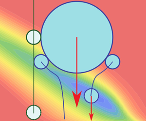
We consider that both drops are entrained by the same background fluid velocity and denote by  $\boldsymbol V_i$ their velocity with respect to this background velocity. The aerodynamic interaction is decomposed into a long-range contribution due to viscous stress, computed using the Oseen approximation, and a short-range contribution due to pressure, computed in the lubrication approximation, as shown in figure 4. We neglect the gradients of velocity at the scale of $R_1$ and $R_2$. We denote by $H=|\boldsymbol r_2-\boldsymbol r_1|-R_1-R_2$ the distance between drops. We consider the Oseen approximation, valid at Reynolds number ${\mathcal {R}}_i \ll 1$. The equation of motion of drop $i$ reads
 \begin{align} \frac 43 {\rm \pi}R_i^3 \rho_\ell \frac{{\rm d} \boldsymbol V_i}{{\rm d}t} &= \frac 43 {\rm \pi}R_i^3 (\rho_\ell-\rho_g) \boldsymbol g - 6 {\rm \pi}\eta_g R_i\left(1+\frac 38 {\mathcal{R}}_i \right) {\boldsymbol V_i}+\boldsymbol F_{ji} -6 {\rm \pi}\eta_g a^2 \zeta'(H) \dot H \boldsymbol e_{ij} \nonumber\\ &\quad - f_{vdW} \boldsymbol e_{ij} + \boldsymbol F^e + \boldsymbol W_i. \end{align}
The index  $j$ is equal to $2$ for $i=1$ and to $1$ for $i=2$. Inertia in the air flow surrounding the drops is controlled by the Reynolds number of each drop, with $\boldsymbol V_i(t)$ the drop velocity,
 \begin{equation} \mathcal{R}_i=\frac{\rho_g V_i R_i}{\eta_g}. \end{equation}
Here  $\boldsymbol F_{ji}$ is the long-range aerodynamic force exerted by the drop $j$ on the drop $i$,
$i$,  $f_{vdW}$ is the van der Waals interaction and $\boldsymbol F^e$ is the electrostatic force between drops. The correction $3/8 {\mathcal {R}}_i$ to the drag on each drop arises from the Oseen approximation (Batchelor Reference Batchelor2010, p. 244). Consistently, the terminal velocity under gravity, denoted $U^t_i$, obeys
 \begin{equation} \left(1+\frac{3 \rho_g R_i U^t_i}{8 \eta_g} \right) U^t_i = \frac{ 2 (\rho_\ell-\rho_g) g R_i^{2}} {9 \eta_g}. \end{equation}
For water drops in air, the associated Reynolds number  ${\mathcal {R}}_i$ reaches $1$ around a radius $R_i\simeq 56\ \mathrm {\mu }{\rm m}$. The term $6 {\rm \pi}\eta _g a^2 \zeta '(H) \dot H \boldsymbol e_{ij}$ is the generic form of the lubrication force originating from the pressure between the two drops. The function $\zeta$ is derived in § 3.2. The dimensionless parameter controlling the relative influence of inertia and viscous damping is the Stokes number, defined here as
 \begin{equation} St\equiv \frac{\rho_\ell a (U^t_1-U^t_2)}{\eta_g}. \end{equation}
Consider two drops of sizes in the same range, say  $R_1=2R_2=3a$. In the viscous aerodynamical regime (Stokes drag), the Stokes number simplifies into $St = \frac 32 \mathcal {G}^3$. The dimensionless number $\mathcal {G}$ can therefore be interpreted as a Stokes number at the terminal velocity, to a power $1/3$. Here $\mathcal {G}$ characterises the influence of inertia for a drop falling around the equilibrium between gravity and viscous friction. The low-Stokes-number regime, where inertia is negligible, is referred to as the overdamped regime. Overdamped dynamics is described by (2.11) without the acceleration term on the left-hand side, i.e. assuming force balance at all times.
In the equations of motion,  $\boldsymbol W_i$ is the thermal noise, delta-correlated in time. The noise is normalised using the fluctuation–dissipation theorem described in § 5. When particles are far apart, it leads to a relative diffusion of the two droplets with a diffusion coefficient
 \begin{equation} D=\frac{k_B T}{6 {\rm \pi}\eta_g a}. \end{equation}
The relative amplitude of aerodynamic effects and thermal diffusion is controlled by the Péclet number, defined as
 \begin{equation} Pe = \frac{(R_1+R_2)(U^t_1-U^t_2)}{D}. \end{equation}
The diffusive regime, where Brownian motion dominates, corresponds to the low-Péclet-number asymptotics.
2.3. Diffusive, electrostatic and inertial regimes
Figure 1(a) is adapted from the classical textbook of Pruppacher & Klett (Reference Pruppacher and Klett2010, chap. 15). It shows the collisional kernel  $K$ between drops of size $R$ with one drop of size 1 $\mathrm {\mu }$m. Multiplied by the number of drops of radius $R$ per unit volume, $K$ gives the collision frequency of a 1 $\mathrm {\mu }$m drop with drops of size $R$. The figure shows a gentle cross-over between Brownian coagulation and gravitational coagulation for drops around $R\simeq 2\ \mathrm {\mu } {\rm m}$. Figure 1(b) presents our results for the same problem. The dot-dashed blue line shows the results obtained when taking into account gravity and aerodynamics only. Below $R=10\ \mathrm {\mu } {\rm m}$, the kernel is ten times smaller than that in panel (a) but above $R=10\ \mathrm {\mu } {\rm m}$, it increases much faster. The dashed red line takes into account van der Waals interaction between drops. Finally, the full model, including Brownian motion is shown in solid green line. The diffusive regime, for $R<1\ \mathrm {\mu } {\rm m}$ is similar to that in figure 1(a). However, in between $R=1\ \mathrm {\mu } {\rm m}$ and $R=10\ \mathrm {\mu } {\rm m}$, the dominant effect turns out to be van der Waals forces.

Figure 1. A change of conceptual model. (a) Graph adapted from the textbook of Pruppacher & Klett (Reference Pruppacher and Klett2010, chap. 15), showing the current vision in cloud microphysics. Comparison between two collisions modes for a spherical particle of 1  $\mathrm {\mu }$m interacting with a second particle of radius $R$, showing a cross-over between Brownian coagulation (green solid line) and gravitational coagulation (dot-dashed blue line). The calculations are based on Klett (Reference Klett1975) and Hidy (Reference Hidy1973). (b) Predictions made here, including gravity, inertia and aerodynamics (dot-dashed blue line), adding van der Waals interactions (dashed red line) and, then, Brownian diffusion (green solid line). A new regime appears between the diffusive regime and the inertial regime, where electrostatic effects become dominant.
As mentioned previously,  $K$ must be multiplied by the number density of drops of size $R$ to obtain the collision frequency with drops of size 1 $\mathrm {\mu }$m. As the density of drops generally decays rapidly with $R$, figure 1 must be interpreted with caution. The quasi-plateau in the purely diffusive regime corresponds, once weighted by the density, to a decrease of Brownian coagulation rate with $R$.
$R$.
In figure 2, the contributions of the dynamical mechanisms to the collision rate is analysed as a function of the two key dimensionless numbers: the Stokes number and the Péclet number. The ratio  $\varGamma$ of the sizes of the large and small drops is kept constant. This measures the relative change of collision rate when one dynamical mechanism is suppressed. The dot-dashed blue line is obtained using overdamped equations (no inertia). It shows that above a Stokes number $St$ on the order of $10$ inertia is dominant. Suppressing it completely changes the collision rate. Similarly, the solid green curve is obtained by suppressing the thermal noise from the equations of motion and shows that below a Péclet number $Pe$ of unity, Brownian coagulation is dominant. Over three decades in drop size $a$, both inertia ( ${St}<1$) and thermal noise ( ${Pe}>1$) are inefficient, so that a third mechanism becomes dominant: electrostatic interactions. One observes that removing the van der Waals forces changes the collision rate by $50\,\%$ (dashed red line). The gap between the diffusive and inertial regimes constitutes the central result of this paper.

Figure 2. Effect of the various dynamical mechanisms on the collision rate for  $\varGamma = R_1/R_2 = 5$. Solid green line: difference in the collision rate with and without thermal diffusion, compared with the collision rate with diffusion, as a function of the Péclet number (top axis). Dash-dotted blue line: difference in the collision rate with and without inertia, compared with the collision rate with inertia, as a function of the Stokes number (bottom axis). Inertia dominates at $St>1$ whereas thermal diffusion dominates at $Pe<1$, leaving $3$ decades in $St$ where neither inertia nor thermal diffusion are relevant. Dashed orange line: difference in the collision rate with and without van der Waals interactions, compared with the collision rate with van der Waals interactions. Lubrication is the dominant effect to reduce the collision rate between the diffusive and inertial regimes. van der Waals interactions limits this gap, but only accounts for a fraction of it.
2.4. Experimental data
Figure 3 compares the collision efficiencies modelled here with experimental data from the literature. Experimental efficiencies roughly collapse on a master curve when plotted as a function of the Stokes number  ${St} = \rho _\ell a (U_1^t-U_2^t)/\eta _g$. They show a drop in efficiency when inertia becomes comparable to aerodynamic effects, as predicted here and in most numerical works since Langmuir (Reference Langmuir1948). The efficiency decreases when the smaller drop does not have enough inertia to cross the streamlines around the larger drop. Efficiencies for $\varGamma$ close to $1$ are less reliable and do not follow this trend, as the small velocity difference means that the drops interact for very long times that may not be reached experimentally. The most accurate experiment is that by Vohl et al. (Reference Vohl, Mitra, Wurzler, Diehl and Pruppacher2007), who used a single collector drop in a controlled airflow at its terminal velocity. The inset of figure 3 shows the Stokes number for which $E=0.2$ (red dotted line) as a function of $\varGamma$. These measurements overlap with our computations for $\varGamma <10$. For larger size ratios, the experimental data rather follows the critical Stokes number for head-on collisions given by (3.24). Unfortunately, efficiencies around the minimum for ${St}=1$ (i.e. 6 $\mathrm {\mu }$m) have never been measured experimentally, nor below this cross-over value. This presents its own experimental challenges, as the critical impact parameter near the minimum is at nanometre scale. Further experimental work is needed to understand the fine details of the collision in the parameter range for which the collision frequency drops, the regime most relevant to cloud microphysics (Beard & Ochs Reference Beard and Ochs1993).

Figure 3. Experimental dataset of the collision efficiency corrected for diffusion  $E_d$ as a function of the Stokes number $St = \rho _\ell a (U_1^t-U_2^t)/\eta _g$. Colour indicates radius ratio $\varGamma =R_1/R_2$. The dash-dotted green line is the computed curve in the absence of an electric field for $\varGamma =5$. Inset: transitional Stokes number as a function of the radius ratio $\varGamma$. Dashed blue line: critical Stokes number $St_\varLambda$ for head-on collisions given by (3.24), with $\varLambda = 4.7$. Dotted red line: Stokes number for the full model at which the efficiency reaches $E=0.2$ in the inertial regime. Crosses: Stokes number for which $E=0.2$ obtained from fitting $\varGamma$-aggregated data from Vohl et al. (Reference Vohl, Mitra, Wurzler, Diehl and Pruppacher2007) to the full model presented here. Agreement is good for $\varGamma <10$ but degrades at larger size ratios. The simple head-on collision model (3.24) captures well the observed trend in the experimental data.
3. Inertial regime
We first revisit the inertial regime, neglecting both electrostatic interactions and Brownian motion. This section is therefore devoted to aerodynamical effects and drop inertia.
3.1. Long-range aerodynamic interactions
In first approximation,  $\boldsymbol F_{ji}$ can be deduced from the effective velocity induced by the drop $j$ at the location of the drop $i$ considered. The drag force can be linearised with respect to the velocity difference between the drop and the gas. Denoting by $\boldsymbol u(\boldsymbol r)$ the velocity field induced by the drop $j$ and taking into account the Faxén correction to the drag force (Guazzelli et al. Reference Guazzelli, Morris and Pic2012), we get
 \begin{equation} \boldsymbol F_{ji}=6{\rm \pi} \eta_g R_i \left(1+\frac 34 {\mathcal{R}}_i \right) \left(\boldsymbol u+\frac 16 R_i^2 {\boldsymbol \nabla}^2 \boldsymbol u\right)_{\boldsymbol r_i}. \end{equation}
The Oseen solution is obtained by linearising the equations around the mean flow. The polar coordinate system is centred on the drop  $j$ inducing the field. Here $\theta =0$ is the direction of the velocity vector $\boldsymbol V_j$. The radial velocity $u_r$ and the tangential velocity $u_\theta$ are given by
 \begin{equation} u_{r} =\frac{1}{r^{2} \sin \theta} \frac{\partial \varPsi}{\partial \theta} \quad {\rm and} \quad u_{\theta} ={-}\frac{1}{r \sin \theta} \frac{\partial \varPsi}{\partial r}, \end{equation}
where the stream function reads (Lamb Reference Lamb1911)
 \begin{align} \varPsi&={-}V_j R_j^{2} \sin ^{2} \theta \frac{R_j}{4 r}+\frac{3 V_j R_j^{2}}{2{\mathcal{R}}_j}(1-\cos \theta)(1-\phi_j ), \nonumber\\ &\qquad\mathrm{with}\ \phi_j\equiv \exp \left(-\frac{r {\mathcal{R}}_j}{2 R_j}(1+\cos \theta)\right). \end{align}
The velocity field reads
 \begin{gather} \frac{u_r}{V_j} ={-}\frac{R_j^{3} \cos \theta}{2 r^{3}}+\frac{3 R_j^{2}}{2 r^{2} {\mathcal{R}}_j}(1-\phi_j ) -\frac{3 R_j(1-\cos \theta)}{4 r} \phi_j, \end{gather}
 \begin{gather}\frac{u_\theta}{V_j} ={-}\frac{R_j^{3} \sin \theta}{4 r^{3}}-\frac{3 R_j \sin \theta}{4 r} \phi_j. \end{gather}
The solution presents an intermediate asymptotics which coincides with the Stokes solution, the velocity field decaying as  $r^{-1}$. However, at distances much larger than $R_j/{\mathcal {R}}_j$, the solution decays much faster, as $r^{-2}$. The Faxén correction requires the evaluation of the Laplacian:
 \begin{gather} \nabla^2 \boldsymbol u |_r ={-}\frac{3 (2R_j+r {\mathcal{R}}_j) (r {\mathcal{R}}_j \sin ^2\theta+4 R_j \cos \theta)}{8R_j r^3} \phi_j, \end{gather}
 \begin{gather}\nabla^2 \boldsymbol u |_\theta ={-}\frac{3 \sin \theta (4R_j^2+ r {\mathcal{R}}_j (2R_j+r {\mathcal{R}}_j)(1+\cos \theta))}{8 R_j r^3} \phi_j. \end{gather}
3.2. Lubrication force
For rigid spheres, the gap  $h(r)$ between the drops can be locally expanded as
 \begin{equation} h(r) = H+R_1+R_2-\sqrt{R_1^2-r^2}-\sqrt{R_2^2-r^2}\simeq H+ \frac{r^2}{2a} \end{equation}
as shown in figure 4(b). In order to regularise the lubrication force, we first introduce the slip length, which is approximately equal to the mean free path  $\bar \ell$ in a gas. Slip at the interface is taken into account using the Navier slip boundary conditions $u_r = \bar \ell \,{\rm d} u_r/{\rm d}z$ at $z = 0$ and $u_r = -\bar \ell \,{\rm d} u_r/{\rm d}z$ at $z = h$. Using cylindrical coordinates, the velocity profile, in the lubrication approximation, reads
 \begin{equation} u_r=\frac{1}{2 \tilde \eta_g} \partial_{r} P (z^{2}-(z+\bar \ell) h), \end{equation}
where  $\tilde \eta _g$ is an effective viscosity which is equal to the viscosity $\eta _g$ at large $H/\bar \ell$, but which gets smaller in the Knudsen regime $H/\bar \ell <1$ (figure 4c). Following Sundararajakumar & Koch (Reference Sundararajakumar and Koch1996), a good approximate expression of $\tilde \eta _g$ is
 \begin{equation} \tilde \eta_g=\frac{\eta_g}{1-\dfrac{2}{\rm \pi} \ln\left(\dfrac{3H}{3H+\bar \ell}\right)} \simeq \frac{\eta_g}{\upsilon}, \quad\mathrm{with}\ \upsilon=1+\frac{2}{\rm \pi} \ln\left(1+\frac{\bar \ell}{3H}\right). \end{equation}
The continuity equation integrates into  $\int _0^h u_r \,{\rm d}z=- r \dot H /2$. Integrating a second time, one obtains the pressure field, which reads
 \begin{equation} P=3\eta_g a \zeta''(h)\dot H, \quad\mathrm{with}\ \zeta''(h)={-}\frac{1}{ 3 \upsilon \bar \ell} \left(\frac{1}{ h}+\frac{1}{6 \bar \ell}\log \left(\frac{h}{6 \bar \ell+h}\right) \right). \end{equation}
The lubrication force is obtained by integrating the pressure over the surface:
 \begin{align} F&\simeq \int_{0}^{\infty} 2{\rm \pi} r P(r) \,{\rm d}r={-}6 {\rm \pi}\eta_g a^2 \zeta'(H) \dot H,\nonumber\\ &\qquad\mathrm{with}\ \zeta'(H)=\frac{1}{3 \upsilon \bar \ell} \left[ \left(1+\frac{H}{6 \bar \ell}\right) \log \left(1+\frac{6 \bar \ell}{H}\right)-1\right]. \end{align}
A second dynamical mechanism can lead to a regularisation of the lubrication force: the induction of a motion inside the liquid (figure 4b). Davis et al. (Reference Davis, Schonberg and Rallison1989) have solved this problem for non-deformable drops, as a function of the fluid to gas viscosity ratio  ${\mathcal {N}}$. The integration of the equations giving the pressure profile and the force, taking both the flow inside the drop and the mean free path into account can only be performed numerically. Here, we make use of exact asymptotic results to derive an approximate analytical formula.

Figure 4. Hydrodynamic mechanisms involved in drop collisions. (a) Long-range aerodynamic interaction. (b) Lubrication in the air film near contact. The shear of the squeezing air flow creates a flow inside the drops. (c) When the gap is comparable to the mean free path  $\bar \ell$, rarefaction of the air between the drops leads to partial slip boundary conditions and a lower effective viscosity. (d) The pressure inside the lubrication air film induces a capillary flattening of the interface.
Let us consider both entrainment of the liquid inside the drop, characterised by an interfacial velocity  $u_t$ and a Poiseuille contribution:
 \begin{equation} u_r=u_t+\frac{1}{2 \tilde \eta_g} \partial_{r} P (z^{2}-(z+\bar \ell) h). \end{equation}
In the mass conservation equation, the flux now reads
 \begin{equation} \int_0^h u_r \,{\rm d}z={-}\frac{r}{2} \dot H=u_t h-\frac{\upsilon}{12 \eta_g} h^2 (h+6 \bar \ell) \partial_{r} P. \end{equation}
Using the Green function formalism, the tangential stress  $\sigma _t$ can be related to the tangential velocity $u_t$ by a non-local relationship. Dimensionally, one obtains the scaling law:
 \begin{equation} \sigma_t=\frac{h}{2}\partial_r P \sim {\mathcal{N}} \eta_g \frac{u_t}{\sqrt{ah}}. \end{equation}
Considering this scaling law as a local relationship, the flow inside the drop would lead to a term  $\sim \sqrt {ah}/{\mathcal {N}}$ added to $h+6 \bar \ell$ in (3.14). There are therefore two possible regularisation processes. Slip occurs in the Knudsen regime, below a gap $h\sim \bar \ell$. The cross-over between a dissipation taking place in the lubrication gaseous film and in the drop takes place at $h\sim a/{\mathcal {N}}^2$.
We therefore propose to modify the function  $\zeta '(H)$ giving the force $F$ into
 \begin{equation} \zeta'(H)=\frac{1}{3
\upsilon \bar \ell} \Bigg[ \Bigg(1+\frac{H+s
\sqrt{aH}/{\mathcal{N}}}{6 \bar \ell}\Bigg) \log
\left(1+\frac{6 \bar \ell}{H+s
\sqrt{aH}/{\mathcal{N}}}\right)-1\Bigg],
\end{equation}
\begin{equation} \zeta'(H)=\frac{1}{3
\upsilon \bar \ell} \Bigg[ \Bigg(1+\frac{H+s
\sqrt{aH}/{\mathcal{N}}}{6 \bar \ell}\Bigg) \log
\left(1+\frac{6 \bar \ell}{H+s
\sqrt{aH}/{\mathcal{N}}}\right)-1\Bigg],
\end{equation}
where  $s$ is a constant. When ${\mathcal {N}}$ goes to infinity, one recovers equation (3.12). Letting $a$ go to infinity, one gets the intermediate asymptotics associated with a drop dominated dissipation: $\zeta '(H)={\mathcal {N}}/s\sqrt {aH}$. Identifying with the result obtained by Davis et al. (Reference Davis, Schonberg and Rallison1989) in this limit, we find $s=1.143\cdots \simeq 8/7$.
3.3. Capillary-limited drop deformation
The deformability of the drop is controlled by the liquid–vapour surface tension  $\gamma$. The thermal waves have a negligible amplitude $\sim \sqrt {k_BT/\gamma }\simeq 0.2$ nm so that the relevant deformations can be predicted using aerodynamics. The drop $j$ flattens over an extension $\delta = \sqrt {2 \tilde ah}$ which modifies the curvature $a^{-1}$ into $\tilde a^{-1}$ and the gap between drops $H$ into $\tilde H$. We denote by $u_j(r)$ the disturbance to the interfacial profile of drop $j$. The volume $\sim \delta ^2 u_j$ is assumed small enough not to change the outer radius $R_j$ through the conservation of volume: the inside pressure for drop $j$ remains $2\gamma /R_j$. The gap $h(r)$ is therefore given by (figure 4d)
 \begin{equation} h(r) \simeq H+u_1(r)+u_2(r) \simeq \tilde H+ \frac{r^2}{2\tilde a}, \quad\mathrm{with} \ \tilde H=H+u_1(0)+u_2(0). \end{equation}
The pressure inside the lubrication film reads  $3\eta _g \tilde a \zeta ''(h)\dot H$. Inside the drop $j$, the pressure gradient balances the inertial term associated with the acceleration of the drop. The reference pressure is controlled by the Laplace pressure for the spherical drop, $2\gamma /R_j$. The Laplace equation evaluated at $r=0$ gives the modified curvature:
 \begin{equation} \frac{1}{\tilde a}=\frac{1}{a}-3 \tilde a \zeta''(\tilde H) \frac{\eta_g \dot H}{\gamma}. \end{equation}
It involves the capillary number  ${Ca}=\eta _g \dot H/\gamma$. Integrating once the Laplace equation, one obtains
 \begin{equation} r \left(1-\frac{r^2}{R_j^2}\right)^{1/2} \gamma \frac{{\rm d}u_j}{{\rm d}r} \simeq 3 \tilde a^2 \eta_g \dot H \left(\zeta'(\tilde H)\left(1-\frac{r^2}{R_j^2}\right)^{3/2}-\zeta'(h)\right). \end{equation}
To obtain  $u_j(0)$, one needs to integrate once more this equation, assuming that $u_j$ vanishes far from the contact zone. The term $\zeta '(h)$ leads to a logarithmic term of the form $\zeta '(H)\ln (r)$, which balances the divergence of the first term. In the outer asymptotic $\zeta '(h)\sim 1/h$, the integration can be performed explicitly, leading to $\zeta '(\tilde H)\ln (r/\sqrt {2\tilde ah})$. Using this approximation, one obtains
 \begin{equation} \tilde H\simeq H-3 \left(\ln\left(\frac{R_1R_2}{2 \tilde a \tilde H}\right)-1\right) \tilde a^2 \frac{\eta_g}{\gamma} \zeta'(\tilde H) \dot H . \end{equation}
Equation (3.20) is an implicit equation for  $\tilde H$. It must be solved alongside (2.11) in which $H$ is replaced by $\tilde H$, yielding at the same time a modified drop separation and a small drop deformation given by (3.17).
3.4. Influence of the different forces
The equations of motion governing the relative position of the two drops are integrated numerically using a Runge–Kutta scheme of order  $4$, with an adaptive time step. The equations are made dimensionless using $a=1$, $\eta _g=1$ and $\rho _\ell =1$. The drops are initially at their terminal velocity, at a distance large enough to obtain results insensitive to this initial condition. In the overdamped limit, we explicitly set ${\rm d} \boldsymbol V_i/{\rm d}t = \boldsymbol 0$ in the governing equation (2.11) and integrate the resulting first-order coupled differential equations using also a Runge–Kutta scheme of order $4$. Over the range of parameters where the inertial and overdamped equations can both be integrated accurately, their results are identical when the drops are small enough.
To investigate the effect of the different forces, we first consider head-on collisions. Figure 5(a) shows trajectories in the phase space  $(H, \dot H)$. The solid green line shows the reference case, where all aerodynamic forces are neglected; the relative velocity then remains equal to $U^t_1-U^t_2$. The dotted blue line shows the result of a calculation ignoring the regularisation of the lubrication force by the mean free path. Conditions are chosen to highlight the existence of a size $a$ for which the two drops collide ( $H=0$) at vanishing velocity ( $\dot H=0$). When the lubrication force is removed altogether (dashed orange line), one can observe the effect of long-range aerodynamic interaction at large distances, which tends to lower the impact velocity. Lubrication forces are dominant at short separations as compared with $a$ and greatly lower the impact velocity in the absence of Knudsen effects (dot-dashed blue line). When introducing a finite mean free path $\bar \ell$ (solid black line), the lubrication force is more efficiently regularised at $H<\bar \ell$, leading to a larger impact velocity. Adding capillary deformations of the drops (dotted red line) only has a very small effect on the results in this regime.

Figure 5. Effect of the different forces on head-on collisions. (a) Example of trajectory in the phase space  $\delta V=-\dot H$ vs $H$, illustrating the role of the different forces. The size ratio is $\varGamma ={R_1}/{R_2}=5$. We chose $a\simeq 89.5\bar \ell$ in the critical condition for the integration performed with the regularisation by the mean free path $\bar \ell$. (b) Normal impact velocity $\delta V=-\dot H$ as a function of the rescaled size $\mathcal {G}$ for $\varGamma = 5$.
Figure 5(b) shows the (normal) velocity at the time of impact as a function of the inertial parameter  $\mathcal {G}$. The impact velocity is always non-zero except when the flow inside both drops is taken into account, but not the finite mean free path $\bar \ell$ (dotted blue line). In this case ( $\bar \ell =0$), the impact velocity vanishes at a critical value of $\mathcal {G}$ below which there is no collision. This critical point is further discussed further in the following. When $\bar \ell$ is taken into account, one observes two regimes: at $\mathcal {G}>1$, the effect of $\bar \ell$ is small and the curve (black line) remains close to the curve presenting a critical point ( $\bar \ell =0$). The effect of capillarity is large for big drops and tends to reduce the impact velocity. It becomes negligible at small $\mathcal {G}$, both because the impact velocity is small and because the drops are less deformable.
3.5. Collision efficiency
When the drops are far from each others, they follow a linear trajectory. We define the impact parameter  $\delta$ as the horizontal distance between these vertical lines. Figure 6(b) shows the normal and tangential velocity as a function of the gap $H/a$ for particular values of $\mathcal {A}$ and $\varGamma$, at the critical impact parameter $\delta _c$. As $\delta$ goes to $0$, one recovers a head-on collision, for which the drops travel in straight lines with a non-zero normal velocity at impact. As $\delta$ increases, the normal velocity decreases and crosses $0$ at this critical impact parameter $\delta _c$. Figure 6(c) shows a critical trajectory, defined by $\delta =\delta _c$, in the frame of reference of the large drop. By definition, the trajectory is tangent at the collision point ( $\dot H=0$ when $H=0$). Comparing this critical trajectory to the ballistic trajectory (figure 6c) allows one to define the collision efficiency as
 \begin{equation} E = \frac{\delta_c^2}{(R_1+R_2)^2}. \end{equation}
Spherical hard particles which do not interact in their trajectory have an efficiency  $E = 1$, by definition. In practice, the limit trajectory is found numerically by bracketing over $\delta _c$ until $\dot H$ vanishes. The initial distance between the drops is chosen large enough to ensure that the results become independent of the choice made; in practice, the required initial distance is around $10^2 R_1$.

Figure 6. (a) Normal impact velocity  $\delta V=-\dot H$ as a function of the impact parameter $\delta$, for $\varGamma =5$ and $\mathcal {A}=75$. (b) Evolution of normal (black solid line) and tangential (red dotted line) velocities as a function of the gap $H$, for the critical value of $\delta$. Here $\varGamma =5$ and $\mathcal {A}=75$. (c) The collision efficiency $E$ is the ration between the geometric collision cross-section and the aerodynamic cross-section. Blue: trajectory for the critical impact parameter $\delta _c = \sqrt {E}(R_1+R_2)$, below which the drops always collide and above which they never do.
Figure 7 shows the collision efficiency  $E$ as a function of the rescaled drop size $\mathcal {A}$, for $\varGamma = 5$. In all cases, the ballistic limit $E = 1$ is recovered for purely inertial drops ( $\mathcal {G} \gg 1$). Ignoring Knudsen effects but taking into account lubrication regularised by flow inside the drops ( $\bar \ell = 0$; dash-dotted blue curve), $E$ vanishes below a critical value of $\mathcal {G}$. At this rescaled scale $a$, the critical impact parameter $\delta _c$ vanishes, which corresponds to the critical head-on collision shown in figure 5. The curve provides a good approximation of the full model (solid black line and dotted red line) above $E\simeq 0.5$ and therefore captures the cross-over value of $\mathcal {G}$ below which the efficiency $E$ drops. The efficiency obtained without any lubrication force is plotted in dotted green line for Stokes long-range flow and in dashed orange line for Oseen long-range flow (figure 7a). Both approximations overestimate the efficiency at $\mathcal {G}<1$ and present a cross-over towards $E=1$ at large $\mathcal {G}$. Oseen flow reduces to Stokes flow above the small drop $2$ (downstream of it). On the opposite, below the large drop, labelled $1$, the flow velocity decays faster (as $r^{-2}$) for the Oseen approximation than for the Stokes approximation (as $r^{-1}$). As a consequence, the large drop $1$ repels less the small drop $2$ using the Oseen approximation so that the efficiency is higher. At small rescaled size $\mathcal {G}$, inertia becomes negligible, as confirmed by the overdamped curve (dash-dotted red curve). As the efficiency decreases with $\mathcal {G}$, the efficiency presents a minimum in the cross-over towards the inertial regime. This suggests decomposing $E$ as the sum of two contributions, as shown in figure 7(b): an overdamped part, which can be accurately computed at vanishing inertia; and an inertial part, defined as the difference to the full calculation. Capillarity deformation of the drops turns out to be negligible in the whole range of parameters. This is due to the fact that, by construction, the efficiency curves are determined from very particular trajectories which have a vanishing normal velocity when colliding.

Figure 7. (a) Collision efficiency for  $\varGamma = 5$ as a function of the dimensionless effective radius $a/\bar \ell$ taking into account different mechanisms. Red dotted line: full solution: inertial dynamics, long-range Oseen interaction, lubrication with drop shear flow, Knudsen effects and capillarity. Dot-dashed: overdamped dynamics. Orange dashed: long-range Stokes interaction, no lubrication. Green dashed: long-range Oseen interaction, no lubrication. Blue dot-dashed: full solution at vanishing mean free path. (b) Decomposition of the collision efficiency (black curve) as the sum of the efficiency computed in the overdamped limit (red dot-dashed curve) plus a remainder, reflecting the inertial limit (blue curve).
In order to understand the origin and the value of the minimum collisional efficiency, we make use of the decomposition of  $E$ into the sum of an overdamped (figure 8a) and an inertial (figure 8b) contribution to the efficiency. In the limit $\varGamma \gg 1$, the smallest drop follows the streamlines around the large drop moving at its terminal velocity. The stream function $\psi (r, \theta ) \simeq - U_1^t r^2 \sin ^2(\theta )(1/2-3R_1/4r+R_1^3/4r^3)$ is therefore approximately constant all along the trajectory, if it is small enough to be in the overdamped regime. Initially the drops are at large distance $r$ such that $r \sin (\theta )\sim \delta$ so that $\psi = - U_1^t \delta ^2/2$. The collision happens at angle ${\rm \pi} /2$ at distance $r = R_1+R_2$. Equating these two values of $\psi$ gives $E=\frac {3}{2} \varGamma ^{-2}$ at asymptotically large $\varGamma$. In figure 8(a), the product $\varGamma ^2 E$ is therefore plotted as a function of $\mathcal {A}$ for different $\varGamma$. At large $\varGamma$, the curves collapse on a single master curve which tends to $1$ (and not $3/2$) in the limit of vanishing $\mathcal {A}$. The lubrication force acts only very close to contact so that the smaller drop eventually leaves its initial streamline. This leads to the smaller prefactor observed, with a scaling still controlled by the long-range forces.

Figure 8. Decomposition of the collision efficiency  $E$. (a) Overdamped contribution: $\varGamma ^2 E$ as a function of $\mathcal {A}$, for six values of $\varGamma$: $1.1$, $4$,
$4$,  $10$,
$10$,  $100$, $500$ and $1500$. At asymptotically large $\varGamma$, the curves tend to a master curve. (b) Inertial contribution, defined as the difference between the efficiency and its overdamped contribution.
The inertial contribution to the efficiency  $E$ is shown in figure 8(b). For asymptotically large $\varGamma$, the drop labelled $1$ is much bigger than the second drop. A change of efficiency is expected at a change of aerodynamical regime of the large drop. As $R_1=a (1+\varGamma )$, one expects that the efficiency is asymptotically controlled by the combination of parameters $\mathcal {G} (1+\varGamma )$. Although far to be a perfect collapse, one observes in figure 8(b) much smaller variations of the inertial contribution to the efficiency, when plotted vs $\mathcal {G} (1+\varGamma )$. This inertial contribution presents similarities with the efficiency obtained in the limit $\bar \ell \to 0$, which vanishes below a threshold. It is therefore interesting to investigate the origin of this threshold. Figure 9(a) presents initial (dotted lines) and collisional velocities (solid lines) for head-on collisions for different $\varGamma$. The impact velocity, above the threshold, remains close to the velocity difference $U_1^t-U_2^t$. The lubrication term controls the dynamics of drops immediately before collision. Let us consider the head-on collision of two drops of mass $m_1$ and $m_2$ and let us neglect gravity and the long-range aerodynamic force. There is no inertia in the gas so that the force on the drops obeys the reciprocal action principle. As a consequence, the two-body problem reduces to a single-body problem with an effective mass $m_1m_2/(m_1+m_2)=\frac {4}{3}{\rm \pi} \rho _\ell \mu a^3$ (with $\mu = (R_1+R_2)^3/(R_1^3+R_2^3)$) with the full force. The dynamical equation reads
 \begin{equation} \tfrac{4}{3}{\rm \pi} \rho_\ell \mu a^3 \ddot H={-}6 {\rm \pi}\eta_g a^2 \zeta'(H) \dot H. \end{equation}
This equation integrates into
 \begin{equation} \frac{\rho_\ell a \Delta \dot H}{\eta_g}={-} \frac{9}{2\mu } \Delta \zeta(H), \end{equation}
where  $\Delta$ denotes the variation between the initial and final states considered, and $\zeta (H)$ is the antiderivative of $\zeta '(H)$.

Figure 9. Head-on collisions and non-continuum effects. (a) Normal impact velocity  $\delta V=-\dot H$ without non-continuum effects as a function of the rescaled drop size $\mathcal {G}$. The radius ratio is $\varGamma ={R_1}/{R_2}=5$. Solid lines: impact velocity in the limit $\bar \ell \to 0$, i.e. without non-continuum effects. Dashed lines: initial velocity. Dotted lines: difference between the impact velocity in the presence of long-range forces only, without any lubrication, and the analytical criterion (3.24), with $\varLambda = 4.7$. (b) Critical value of $\mathcal {G}$ below which the impact velocity vanishes before collision, for different long-range forces. Solid black line: Stokes long-range force (with $\bar \ell \to 0$). Solid red line: Oseen long-range force (with $\bar \ell \to 0$). Dotted green line: criterion of (3.24) with $\varLambda = 17.4$. Solid orange line: isocurve of efficiency $E = 0.2$, including non-continuum effects. Solid purple line: efficiency minimum $\mathcal {G}_{min}$, including non-continuum effects.
As a consequence, the lubrication film prevents the collision of drops with an insufficient initial velocity difference. The precise criterion in the absence of long-range forces is a threshold Stokes number
 \begin{equation} {St}_\varLambda\equiv \frac{\rho_\ell a (U^t_1-U^t_2)}{\eta_g}=\frac{9}{2\mu}\varLambda, \end{equation}
where  $\varLambda = \int \zeta '(H)\,\mathrm {d} H$ is a logarithmic factor originating from the fact that, at large $H$,
$H$,  $\zeta '(H) \sim H^{-1}$. Here $\varLambda$ depends on the dynamical mechanism regularising the lubrication pressure. Figure 9(a) shows in dotted lines the impact velocity obtained by subtracting equation (3.24) from the impact velocity computed only with long-range interactions, in the absence of lubrication forces. The good agreement with the full calculation, with long-range forces, using a constant $\varLambda = 4.7$ shows that there is scale separation between the near-contact lubrication and the long-range interactions.
In the viscous drag regime in which (2.13) reduces to  $U_i^t = 2(\rho _\ell - \rho _g)gR_i^2/9\eta _g$, the threshold given by (3.24) can be expressed as $\mathcal {G}= \mathcal {G}_\varLambda$, with
 \begin{equation} \mathcal{G}_\varLambda=\left(\frac{81}{4} \varLambda \frac{\varGamma^2 (1+(\varGamma-1) \varGamma)}{(\varGamma-1) (1+\varGamma)^5}\right)^{1/3}. \end{equation}
Surprisingly, this scaling is close to the scaling obtained with Oseen long-range forces [solid red line in figure 9b]. Stokes long-range forces (solid black line) displays completely different behaviour as the  $r^{-1}$ interaction makes the impact velocity much smaller than the terminal velocity difference over the whole range of $\mathcal {G}$.
This sheds light on the behaviour of the efficiency near its fast inertial decrease and minimum. The values of  $(\varGamma, \mathcal {G})$ for which $E = 0.2$ are shown as the orange line in figure 9(b). For that iso-efficiency curve, $\mathcal {G}$ follows the scaling $\mathcal {G} \propto \varGamma ^{-1}$ at large $\varGamma$. The value of the minimum of $E$,
$E$,  $\mathcal {G}_{min}$, decreases faster as $\varGamma ^{-2}$. Figure 10(a) provides a summary of the relationship between collisional efficiency and the size of both droplets.

Figure 10. Isocontours of the collision efficiency  $E$ as a function of $\varGamma$ and $\mathcal {A}$. Dashed line: minimum value of the collision efficiency for at a given $\varGamma$. All aerodynamical effects are taken into account. Parameters are those of water droplets. For large sizes and aspect ratios, geometric behaviour is recovered. Below a certain Stokes number $\mathcal {G}$, the efficiency decreases very rapidly and reaches a minimum. (a) Without van der Waals interactions. (b) With van der Waals interactions. The efficiency rapidly decreases from the geometric value when inertia is low enough, in the same way as in the purely aerodynamic case. Van der Waals interactions increase the minimum efficiency by a factor $10$. Collisions in the overdamped regime are also more efficient, leading to a narrower valley of collision slowdown.
4. Electrostatic regime
4.1. Electrostatic interactions: van der Waals and Coulombian forces
The average droplet charge for weakly electrified clouds is  $\sim e$ (Harrison, Nicoll & Ambaum Reference Harrison, Nicoll and Ambaum2015). When the drops are far apart, they interact as two point charges $q_1$ and $q_2$ by the electrostatic potential energy $q_1 q_2/4{\rm \pi} \varepsilon r$, where $\varepsilon$ is the air permittivity. The electric force can either be repulsive or attractive depending on the relative charges. In the case of clouds, one rather expects all drops to present the same sign, hence leading to a repulsion. The electrostatic force $F_e$ becomes comparable with the lubrication force $\propto \eta _g a^2 U^t/h$ driven by $U^t = 2/9 \rho _\ell g a^2/\eta _g$ at separations $h_e \sim q^2/(4{\rm \pi} \varepsilon \rho _\ell g a^4)$. $h_e$ is comparable to the mean free path $\bar \ell$ for $a = 0.5$ $\mathrm {\mu }$m and decreases very rapidly with $a$. In disturbed weather, storm clouds develop large electric fields, the bulk of the cloud becomes negatively charged and drops carry much larger charges, up to $10^5\;e$ (Takahashi Reference Takahashi1973). Here, we restrict our analysis to electroneutral drops, which is a good approximation in the bulk of warm clouds (Pruppacher & Klett Reference Pruppacher and Klett2010, chap. 18).
Van der Waals forces between drops can be computed using the unretarded van der Waals pair potential. At very small separation, the disjoining pressure  $\varPi (h)$ is given by the phenomenological expression involving the Israelashvili length $\varsigma$:
 \begin{equation} \varPi(H)={-}\frac{4 \gamma \varsigma^2}{(\varsigma+H)^3}. \end{equation}
This formula obeys the integral relation giving the surface tension:  $\int _0^\infty \varPi (h) \,{\rm d}h=-2\gamma$. Moreover, at intermediate $H$ large with respect to the molecular scale, but small with respect to $a$, one recovers the decay as $\varPi (H) \sim -4 \gamma \varsigma ^2/H^3$. The force is given by integrating the disjoining pressure over the surface:
 \begin{equation} f^{vdW}=\int_{0}^{\infty} 2{\rm \pi} r \varPi(h) \,{\rm d}r={-}4{\rm \pi} \gamma a \frac{\varsigma^2}{(\varsigma+H)^2}. \end{equation}
This expression holds at gap  $H$ comparable to $\varsigma$. Hamaker (Reference Hamaker1937) showed that at all separations,
 \begin{equation} \boldsymbol f_{ji}^{vdW} ={-}A \frac{32 R_1^3 R_2^3 (R_1+R_2+H)}{3(2 R_1+H)^2 (2 R_2+H)^2 (2 (R_1+R_2)+H)^2 (H+\varsigma)^2} \boldsymbol e_{ij}, \end{equation}
where  $A=3.7\times 10^{-20}$ J is the Hamaker constant. It matches with (4.3) in the small $H$ limit, since $\varsigma =\sqrt {A/(24{\rm \pi} \gamma )}$. Note that the molecular cut-off length $\varsigma$ is equal to $0$ in the original work of Hamaker (Reference Hamaker1937). At large distances, the van der Waals force asymptotically tends to
 \begin{equation} f^{vdW} ={-}A\frac{32 R_1^3 R_2^3 }{3H^7}. \end{equation}
4.2. Vertical static electric field
Fair weather clouds, which do not develop their own strong electric fields, are electrified at their boundaries, with a positive charge at cloud top and a negative charge at cloud base (Harrison et al. Reference Harrison, Nicoll and Ambaum2015). This can be modelled as a vertical electric field  $\boldsymbol E_0$, as shown in figure 12(a). The drops act as conducting spheres and behave as induced dipoles of dipolar moment $\boldsymbol p_i=4 {\rm \pi}\varepsilon R_i^3 \boldsymbol E_0$. When the drops are far from each others, the electric potential around the drop $j$ obeys the Poisson equation and takes the form
 \begin{equation} V(r, \theta)=E_0 r \cos \theta\left(\frac{R_j^3}{r^3}-1\right). \end{equation}
The force exerted on the other drop, labelled  $i$, derives from the energy $\boldsymbol p_i \boldsymbol {\cdot } \boldsymbol \nabla V$:
 \begin{gather} F_r={-}12 {\rm \pi}\varepsilon E_0^2 (R_iR_j)^3\frac{2 \cos^2 \theta-\sin^2 \theta}{(R_1+R_2+H)^4}, \end{gather}
 \begin{gather}F_\theta={-}12 {\rm \pi}\varepsilon E_0^2 (R_iR_j)^3\frac{\sin (2 \theta)}{(R_1+R_2+H)^4}. \end{gather}
At small separations, however, the force must be corrected for the geometrical amplification of the field in the gap separating the two drops. This effect presents similarities with the lubrication discussed previously. For practical purpose, the exact solution derived by Davis (Reference Davis1964) can be approximated by the following phenomenological formula:
 \begin{gather} F^e_r={-}12 {\rm \pi}\varepsilon E_0^2 (R_iR_j)^3\left( \frac{2 \cos^2 \theta}{(c_c+H)^{3+\alpha}H^{1-\alpha}}-\frac{\sin^2 \theta}{(c_s^2+H^2)(c_s+H)^2)}\right), \end{gather}
 \begin{gather}F^e_\theta={-}12 {\rm \pi}\varepsilon E_0^2 (R_iR_j)^3\frac{\sin (2 \theta)}{(c_\theta+H)^{4-\alpha}(c_\theta^\alpha+H^\alpha)}, \end{gather}
with  $\alpha \simeq 0.2$, $c_c\simeq 1.36 (R_1+R_2)$, $c_s\simeq 1.55(R_1+R_2-a)$ and $c_\theta \simeq 0.77(R_1+R_2)$ and the notation of figure 12(a). It provides a good fit to the exact force down to $H\simeq 10^{-6} a$.
4.3. Results
Figure 11(a) compares the efficiency curves obtained with and without the van der Waals interaction forces. To a first approximation the curves are superimposable in the inertial zone but, in the overdamped regime, the attractive interactions lead to a significantly higher collision efficiency than without. The decrease in efficiency at small size  $a$ is mainly due to the lubrication layer, but the residual efficiency for near-frontal collisions is significantly affected by the subdominant van der Waals interactions. In particular, the efficiency minimum is shifted by a factor $2$ in size $a$, and is almost 10 times larger when the attractive intermolecular interactions are taken into account.

Figure 11. (a) Decomposition of the collision efficiency (black curve) as the sum of the efficiency computed in the overdamped limit (red dot-dashed curve) plus a remainder, reflecting the inertial limit (blue curve), with and without van der Waals interactions. (b) Collision efficiency  $E$ for $\varGamma = 5$ as a function of the dimensionless effective radius $a/\bar \ell$ for different values of the Hamaker constant: $A=0$ (red line), $A=3.7\times 10^{-21}$ J (green line), $A=3.7\times 10^{-20}$ J (blue line), which is the value for water, $A=3.7\times 10^{-19}$ J (purple line) and $A=3.7\times 10^{-18}$ J (black line).
Figure 11(b) compares the efficiency curves obtained for different values of the Hamaker constant. It can be seen that the inertial component of the efficiency remains practically unchanged. The more attractive the interactions are, the more efficient the collisions are in the overdamped regime. It can be observed that the curves obtained are parallel: the efficiency presents an asymptotic behaviour with the scaling law  $E \propto \mathcal {T}^{0.8}\mathcal {A}^{-1.7} \varGamma ^{-1}$.
Figure 12(b) compares the efficiency curves obtained for different values of a vertical electric field, ignoring this time the van der Waals forces associated with permanent dipoles. Similarly to the curves obtained with van der Waals interactions, the curves overlap in the inertial regime and differ only in the overdamped regime, where a stronger electric field leads to an enhanced collision rate. The efficiency minimum scales as  $E_{min} \propto (\mathcal {E}^2)^{0.8}$, as the force $F^e$ is quadratic in the field $\mathcal {E}$. This is similar to the scaling obtained only with van der Waals interactions as $\mathcal {T}^{0.8}$ with a scaling exponent below $1$, reflecting the balance between lubrication and attractive electrostatic forces below the inertial regime.

Figure 12. (a) Minimum efficiency  $E_{min}$ for $\varGamma = 2$ as a function of the dimensionless electric field $\mathcal {E}$. Inset: schematic of the forces created by the static vertical field $\boldsymbol E_0$. The electrostatic force can be decomposed into a radial part $F_r^e$ and an orthoradial part $F_\theta ^e$ given by (4.8) and (4.9). (b) Collision efficiency $E$ for $\varGamma = 2$ as a function of the dimensionless effective radius $a/\bar \ell$ for different values of $\mathcal {E}$, ranging from the typical value in non-precipitating warm clouds ( $10^{-3.5}$) to a fraction of the breakdown field $\mathcal {E} \simeq 6$.
For a typical non-precipitating cloud,  $\mathcal {E}$ is around $10^{-3.5}$ ( $E_0 = 0.15$ kV m $^{-1}$), which is far too small to lead to a significant effect. One observes that the effect of electrostatics doubles the collisional efficiency for $\mathcal {E} = 10^{-2.5}$ ( $E_0 = 1.5$ kV m $^{-1}$) i.e. for an electric field 10 times larger than the fair weather electric field and $2000$ times smaller than the breakdown electric field ( $\mathcal {E} = 6$; $E_0 = 3\times 10^3$ kV m $^{-1}$). The gap is closed (efficiency is $1$) for an electric field $\mathcal {E} = 1.3\times 10^{-1}$ ( $E_0 = 60$ kV m $^{-1}$) which is $50$ times smaller than the breakdown electric field. In conclusion, a vertical electric field has a negligible effect in non-precipitating cloud but may have a dominant effect for electric fields one order of magnitude larger, but still three orders of magnitude smaller than that observed in thunderclouds.
Figure 10 shows the efficiency  $E$ as a function of the radius ratio $\varGamma$ and the rescaled size $\mathcal {A}$, for water drops in air, on Earth. As $\varGamma$ increases, for very large drops collecting small ones, the minimum of the efficiency decreases as well as the value of $\mathcal {A}$ at which it is realised (dashed line). Without van der Waals interactions, the minimum efficiency is less and less pronounced as the size $a$ increases. By contrast, taking van der Waals interactions into account (figure 10b), the minimum efficiency is (roughly 10 times) larger, but presents a much weaker dependence on the size $a$.
$a$.
5. Diffusive regime
In the previous two sections, we have studied the mechanisms that control the collision efficiency in the athermal limit. In the overdamped, small size regime, we have shown that the dynamics is dominated by the lubrication layer between the drops, with attraction by van der Waals forces and long-range aerodynamic interaction playing a subdominant role. In this regime, another mechanism can play a very important role: Brownian motion. In the theoretical description of droplet aggregation processes, it is generally assumed that the collision rates induced by Brownian motion and those generated by gravity are additive. Here, we study simultaneously the gravitational and Brownian coagulation and test this additivity assumption. We show that thermal diffusion dominates the collision rate below a transitional Péclet number of order unity, but has a subdominant influence in the region of the parameter space which is neither inertial nor diffusive, so that the collision efficiency is minimal. This implies first redefining the collision efficiency by including the effect of thermal noise and gravity simultaneously.
5.1. Normalisation of the thermal noise
We now take into account the thermal noise in the equation of motion (2.11). Following Batchelor (Reference Batchelor1976), we consider that the separation of time scales between the time to return to thermal equilibrium and the time for the particle configuration to change is sufficient to consider the position of the particles as constant when computing the correlations of thermal noises. In the inertial regime, diffusion is negligible. Conversely, in the regime where diffusion is important, inertial effects can be neglected. As a consequence, we use the Stokes model of long-range aerodynamic interactions rather than Oseen's model. Then, the equations for the velocity component along the direction of the axis joining the two particles and those for the two perpendicular components decouple. For simplicity, we single out one such velocity component and introduce the equation governing the velocity fluctuation  $u_i$ along the chosen axis. As thermal diffusion is an Ornstein–Uhlenbeck process, it is convenient to write the Langevin equation under the following form (Risken & Frank Reference Risken and Frank1989), with Einstein summation over indices:
 \begin{equation} \frac{{\rm d} u_i}{{\rm d}t}={-}S_{ij} u_j+ W_i \quad {\rm with}\ \langle W_i(t)W_j(t') \rangle = \mathcal{W}_{ij} \delta(t-t'). \end{equation}
The indices  $i$ and $j$ here refer to the particle number, the three components being considered separately. It is convenient to write the relaxation rate matrix $\boldsymbol {S}$ under the form
 \begin{equation} S_{ij} = \frac{9 \eta_g}{2\rho_\ell R_i^3} \alpha_{ij}. \end{equation}
For the axis joining the centre of the drops, the matrix  $\alpha _{ij}$ reads
 \begin{gather} \alpha_{11}=R_1+ a^2 \zeta'(H),\quad\alpha_{22}= R_2+ a^2 \zeta'(H), \end{gather}
 \begin{gather}\alpha_{12}=\alpha_{21}={-}\frac{R_1R_2 }{2r}\left(3-\frac{R_1^{2} +R_2^{2} }{r^{2}}\right) - a^2 \zeta'(H). \end{gather}
In the plane perpendicular to the axis joining the centre of the drops, it reads
 \begin{gather} \alpha_{11}= R_1,\quad \alpha_{22}= R_2, \end{gather}
 \begin{gather}\alpha_{12}=\alpha_{21}={-}\frac{ R_1R_2 }{4r}\left(3+\frac{R_1^{2} +R_2^{2} }{r^{2}}\right). \end{gather}
The Langevin equation integrates into, summed over indices,
 \begin{equation} u_i= \int_0^t G_{ij}(t-t') W_j(t') \,{\rm d}t', \end{equation}
where  $G_{ij}$ denotes the matrix elements of the Green's function $\boldsymbol {G}$, which formally obeys, in matrix notation, $\boldsymbol {G}=\exp (-\boldsymbol {S} t)$. Similarly, the velocity $u_i$ can be integrated formally to give the position.
The velocity correlation function reads, with Einstein summation,
 \begin{equation} \langle u_i(t)u_j(t) \rangle=\int_0^t G_{ik}(t')G_{jl}(t') \,{\rm d}t' \mathcal{W}_{kl}. \end{equation}
Using the generalised equipartition of energy,
 \begin{equation} \langle u_i(t)u_j(t) \rangle_{t\to\infty}= \frac{3 k T}{4 {\rm \pi}\rho_\ell R_k^3} \delta_{ik}\delta_{jk}, \end{equation}
we deduce
 \begin{equation} \mathcal{W}_{ij}=\frac{3kT}{4 {\rm \pi}\rho_\ell} \left(\frac{S_{ij}}{R_j^3}+\frac{S_{ji}}{R_i^3}\right). \end{equation}
In practice, at each integration step of the Runge–Kutta of order 4 algorithm, noise terms obeying a series of correlation rules described by Ermak & Buckholz (Reference Ermak and Buckholz1980) between positions and velocities are added to the deterministic increments. The fourth-order integration scheme is recovered in the limit where the thermal diffusion is negligible. Conversely, the scheme is designed to lead to the exact diffusion result, when diffusion is dominant, provided the thermal equilibration time scale is smaller than the typical time scale of evolution of the geometrical configuration.
5.2. Redefining the collision efficiency
We have previously defined the collision efficiency as the factor encoding the influence of aerodynamics and electrostatic forces on the collision frequency of particles. The reference frequency was derived in the ballistic limit, in which the two particles of radii  $R_i$ settle with a differential speed $U = U^t_1-U^t_2$, and reads: $\nu = {\rm \pi}(R_1+R_2)^2 n_0 U$. Considering now the effect of thermal noise, the effect of diffusion must be included in the reference collision frequency to which the real rate is compared to define $E$. Each particle diffuses with a diffusion constant $D_i = k_B T/(6{\rm \pi} \eta _g R_i)$. The problem is equivalent to the advection-diffusion of particles with a diffusion coefficient $D = D_1 + D_2$. The diffusion-advection equation for the particle concentration $n$ is, in spherical coordinates,
 \begin{equation} -U \cos\theta \partial_r n + U \frac{\sin\theta}{r}\partial_\theta n = D\left(\frac{1}{r^2}\partial_r (r^2 \partial_r n) + \frac{1}{r^2 \sin\theta}\partial_\theta (\sin\theta \partial_\theta n)\right). \end{equation}
The boundary conditions are  $n(r\to \infty ) = n_0$, $n(r = R_1+R_2) = 0$. The combined effects of diffusive and advective transport on droplet growth are described by the particle flux, i.e. the collision rate, at the drop surface
 \begin{align} \nu_0 &= 2{\rm \pi} D (R_1+R_2)^2 \int_0^{\rm \pi} \mathrm{d} \theta \left(\frac{\partial n}{\partial r}\right)_{r = R_1+R_2} \sin\theta\nonumber\\ &= {\rm \pi}(R_1+R_2)^2 n_0 U\ q({Pe}). \end{align}
In the purely Brownian limit, one gets  $\nu = 4{\rm \pi} D (R_1+R_2) n_0$ so that $q({Pe}) \sim 4/{Pe}$. In the purely ballistic limit, $q({Pe}) \sim 1$. Equation (5.11) has been solved analytically by Simons et al. (Reference Simons, Williams and Cassell1986), and $q({Pe})$ can be expressed as
 \begin{equation} q({Pe}) = \frac{4{\rm \pi}}{{Pe}^2}\sum_{n=0}^\infty ({-}1)^n (2n+1)\frac{I_{n+1/2}\left(\dfrac{Pe}{2}\right)}{K_{n+1/2}\left(\dfrac{Pe}{2}\right)}, \end{equation}
with  $I_n$, $K_n$ the modified Bessel functions. Care must be taken when evaluating this series (Sajo Reference Sajo2008). Consequently, we define the collision efficiency in the presence of diffusion and all aerodynamic effects as the ratio between the collision rate $\nu$ and the reference collision rate ${\rm \pi} (R_1+R_2)^2 n_0 U q({Pe})$:
 \begin{equation} E_d = \frac{\nu}{{\rm \pi} (R_1+R_2)^2 n_0 U q({Pe})}. \end{equation}
In practice, we compute the collision frequency  $\nu$ using a Monte Carlo method. We uniformly sample impact parameters over a square upstream and compute the trajectory for each sample point. The reduced collision rate $\nu /({\rm \pi} (R_1+R_2)^2 n_0 U)$ is estimated by measuring the ratio between the surface area of impact parameters leading to a collision to the area in the geometric case ${\rm \pi} (R_1+R_2)^2$.
5.3. Results
The collision efficiency  $E_d$ is shown for $\varGamma = 5$ without van der Waals forces in figure 13(a). At large inertia ( $\mathcal {G} >1$), the efficiency curve (solid line) collapses with athermal results (dash-dotted line) and there is no effect of diffusion, as expected. At small Péclet number, fully diffusive behaviour ( $E_d \to 1$) is recovered asymptotically. Note that, with the new definition of the efficiency taking into account diffusion, athermal collisions become vanishingly inefficient at small Péclet number. The effect of diffusion is visible at the collision efficiency minimum, even when it is reached at high Péclet numbers ( ${\sim }10^5$) where diffusion would be expected to be negligible at a glance. The effect of Brownian motion on particle growth is often modelled in the literature (Greenfield Reference Greenfield1957) by simply adding together the purely diffusive particle collision rate $4 {\rm \pi}D (R_1+R_2) n_0$ with the purely athermal particle collision rate ${\rm \pi} (R_1+R_2)^2 E U n_0$ computed previously. With the definition of $E_d$ (5.14) proposed there, this leads to
 \begin{equation} E_d^{sum} = \frac{4/{Pe}+E}{q({Pe})}. \end{equation}
Note that 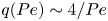 $q({Pe}) \sim 4/{Pe}$ in the small-Péclet-number limit, leading to $E_d^{sum}\to 1$ for ${Pe}\to 0$. The resulting curve (dotted line) does not collapse over the full Monte Carlo solution: diffusion and aerodynamic effects are not additive on particle growth. Results with van der Waals interactions are shown in figure 13(b). Similarly, the purely diffusive and purely ballistic regimes are recovered asymptotically, with diffusion present in the gap. Likewise, the additive model $E_d^{sum}$ does not accurately reproduce the simulation results. Van der Waals interactions and diffusion enhance each other in a non-trivial way near the gap. Figure 14 shows the combined diffusiogravitational efficiency $E_d$ for water drops on Earth as a function of $\mathcal {A}$ and $\varGamma$, with van der Waals interactions. The gap in the efficiency is about $10^{-3}$, and becomes slightly shallower, narrower and shifted to smaller sizes as the size ratio $\varGamma$ of the droplets increases.

Figure 13. (a) Collision efficiency  $E_d$ for $\varGamma = 5$ without van der Waals interactions. (b) Collision efficiency $E_d$ for $\varGamma = 5$ with van der Waals interactions. Solid lines: Monte Carlo simulation of the Langevin equation, with and without van der Waals forces, taking into account thermal noise. Dash-dotted lines: previous athermal efficiency in the new definition of the diffusiogravitational efficiency $E_d$. Dotted lines: additive model for the diffusiogravitational efficiency.

Figure 14. Isocontours of the collision efficiency  $E_d$ as a function of $\varGamma$ and $\mathcal {A}$. Dashed line: minimum value of the collision efficiency at a given $\varGamma$. All aerodynamical effects, van der Waals interactions and thermal diffusion are taken into account. Parameters are those of water droplets. For large sizes and aspect ratios, geometric behaviour is recovered; likewise, for small sizes and aspect ratios, purely diffusive behaviour is recovered. In between the two regimes, there is a valley of lower collision rate where electrostatic effects dominate.
6. Discussion
In this article, we have analysed the influence of relevant dynamical mechanisms on the collision efficiency of drops suspended in a gas. The largest drops, falling under the effect of gravity, merge when their motion is inertial, meaning that their Stokes number  ${St}$ is larger than $1$. The smallest drops have a motion controlled by thermal diffusion, below a unit Péclet number. The main result of this paper is the existence of a range of drop sizes for which neither inertial nor diffusive effects are dominant, resulting in a large decrease of the collision efficiency. In this intermediate regime, it is the gaseous lubrication film separating the drops that prevents them from merging. In addition, van der Waals forces become non-negligible. The code used here allows us to compute the efficiency over the whole size range in clouds, both for equally sized drops and for drops of very different sizes.
As the outcome of a collision is binary (either the droplets merge or they do not), and the growth rate increases rapidly with the drop size, the growth process is extremely sensitive to minute details of the collision. We have neglected here added mass, the Basset/history force, shear, all rotation and torque effects (Maxey & Riley Reference Maxey and Riley1983; Mordant & Pinton Reference Mordant and Pinton2000), but also non-aerodynamic effects such as retardation in the van der Waals force (Gregory Reference Gregory1981), thermophoresis due to temperature gradients and diffusiophoresis due to water vapour gradients (Friedlander Reference Friedlander2000, chap. 3). For millimetric drops, capillary deformations become important around a Weber number of  $1$. Drop deformation flattens the drops, which changes their settling speed and ultimately leads to break-up (Reyssat et al. Reference Reyssat, Chevy, Biance, Petitjean and Quéré2007; Villermaux & Bossa Reference Villermaux and Bossa2009). Capillary instabilities can also be triggered during the collision, leading to the formation of smaller droplets by various fragmentation processes of liquid filaments and sheets (Villermaux Reference Villermaux2007; Testik, Barros & Bliven Reference Testik, Barros and Bliven2011; Testik & Rahman Reference Testik and Rahman2017).
6.1. Stability of fogs and non-precipitating clouds
The problem of raindrop formation can be seen in terms of a dual question. Why don't all droplet dispersions lead to raindrops? Why do, conversely, some warm clouds produce rain? To shed light on this problem, based on the results presented here, let us compute the growth time  $\tau _D$ associated with condensation and the growth time $\tau _C$ associated with the collisional cascade (Figure 15a). Consider a droplet of radius $R$ condensing in an atmosphere of vapour density $\rho _v$. The mass growth rate reads (Pruppacher & Klett Reference Pruppacher and Klett2010, chap. 13)
 \begin{equation} \frac{4{\rm \pi}}{3} \rho_\ell \frac{\mathrm{d} R^3}{\mathrm{d} t} = 4{\rm \pi} D (\rho_v - \rho_{sat}) R. \end{equation}
Let us consider that the number of drops per unit volume  $\psi$ remains constant, fixed by the nucleation rate. The water mass conservation relates $\rho _v$ and $R$ to the initial absolute humidity $\rho _v^0$ by $\rho _v = \rho _v^0 - 4{\rm \pi} \psi \rho _\ell R^3/3$. Steady state is achieved when $\rho _v = \rho _{sat}$, when the radius reaches the value $R_\infty$ set by
 \begin{equation} \psi \frac{4{\rm \pi}}{3} \rho_\ell R_\infty^3 = \rho_v^0 - \rho_{sat}. \end{equation}
The evolution equation (6.1) takes the form
 \begin{equation} \frac{\mathrm{d} R^2}{\mathrm{d} t} = \frac{R_\infty^2}{\tau_D}\left(1 - \frac{R^3}{R_\infty^3}\right), \end{equation}
where the typical condensation growth time  $\tau _D$ obeys
 \begin{equation} \frac{4{\rm \pi}}{3} \psi D R_\infty \tau_D=1. \end{equation}
We introduce here the liquid water content  $\rho _d$, which is the total mass of liquid water per unit volume: $\rho _d = 4{\rm \pi} \psi \rho _\ell R_\infty ^3 /3$. In clouds, $\rho _d$ is typically 0.3 g m $^{-3}$, and can be as high as 3 g m $^{-3}$ in cumulonimbus clouds (Hess et al. Reference Hess, Koepke and Schult1998; Rosenfeld & Lensky Reference Rosenfeld and Lensky1998). We show $\tau _D$ in figure 15 as the solid red line for $\rho _d = 0.3$ g m $^{-3}$. Holding $\rho _d$ constant, the growth time $\tau _D = (\rho _\ell /\rho _d) R_\infty ^2/D$ increases as $R_\infty ^2$: condensation is increasingly slower at forming larger drops. In this theory, $\psi$ is not constrained, and decreases with increasing $R_\infty$ to accommodate the given liquid water content. In practice, $\psi$ is set by the distribution of cloud condensation nuclei, their chemical properties and the dynamics of saturation (Twomey Reference Twomey1959; Ghan et al. Reference Ghan, Abdul-Razzak, Nenes, Ming, Liu, Ovchinnikov, Shipway, Meskhidze, Xu and Shi2011; Kreidenweis, Petters & Lohmann Reference Kreidenweis, Petters and Lohmann2019). This gives a lower bound for $\psi$, around $10^7\ {\rm m}^{-3}$. $\tau _D$ for densities $\psi$ above this value, that are not observed in nature, is shown as a thin line. A very short time, around a few seconds to a few minutes, is therefore needed to reach droplet sizes between $1$ and 10 $\mathrm {\mu }$m by condensation growth alone; larger sizes would require unrealistically low drop densities $\psi$. The drop size distribution produced also tends to be narrow (Brenguier & Chaumat Reference Brenguier and Chaumat2001), as the radius of an individual drop varies as $\mathrm {d} R/\mathrm {d} t \sim 1/R$. The onset of rain formation must consider the collisional growth of nearly equal-sized droplets.

Figure 15. (a) Schematic of the two growth modes in a cloud. Left: condensation growth of a drop of radius  $R_\infty$, driven by the diffusion of excess water vapour in air. Right: the collisional cascade, in which a larger drop of radius $R_1$ collects smaller drops of radius $R_\infty$ as it settles. The larger drop gradually depletes the cloud of its smaller droplets. (b) Growth times $\tau _C$ and $\tau _D$ rescaled by $T_b$ (left axis) or expressed in seconds (right axis) as a function of the cloud droplet size $R_\infty$ rescaled by $b$ (bottom axis) or expressed in $\mathrm {\mu }$m (top axis). Growth time scale $\tau _C$, dash-dotted blue line: athermal model including lubrication force but without van der Waals interactions. Dotted orange line: Brownian model without van der Waals interactions. Solid black line: full prediction. Growth time $\tau _D$ by condensation of water vapour; solid red line: the range of $R_\infty$ corresponding to droplets observed in clouds is shown with a thick line and anomalously low densities $\psi <10^7\ {\rm m}^{-3}$ with a thin line.
Let us now consider a uniform cloud of drops of size  $R_\infty$. The evolution equation for a single drop of size $R_1$, due to coalescence with the drops of size $R_\infty$ smaller than $R_1$, derives from (1.2):
 \begin{equation} 4{\rm \pi} \rho_\ell R_1^2 \frac{{\rm d}R_1}{{\rm d}t}= \rho_d {\rm \pi}(R_1+R_\infty)^2 |U_1^t-U_\infty^t| E_d q({Pe}). \end{equation}
We define the rescaled terminal velocity  $\mathcal {U}(R/b)$ by $U^t = 2 (\rho _\ell -\rho _g)gb^2/9\eta _g \mathcal {U}$ and the typical evolution time scale of drops at the cross-over size $b=\eta _g^{2/3} ( \rho _\ell (\rho _\ell -\rho _g) g )^{-1/3} = 3.3$ $\mathrm {\mu }$m by:
 \begin{equation} T_b = 18 \frac{\rho_\ell (\rho_\ell-\rho_g) b^2}{\rho_d \eta_g}. \end{equation}
For  $\rho _d = 0.3$ g m $^{-3}$, a typical liquid water content in clouds (Pruppacher & Klett Reference Pruppacher and Klett2010, chap. 2), we get $T_b = 9.6$ h. The drop growth time $\tau _C$ in the linear regime $R_1-R_\infty \ll R_\infty$ obeys
 \begin{equation} \frac{T_b}{\tau_C}= 4 E_d q({Pe}) {\mathcal{U}}'(R_\infty/b) . \end{equation}
The rescaled growth time  $\tau _C/T_b$ is shown in figure 15(b) as a function of the cloud drop radius $R_\infty$ in the athermal and Brownian cases. The positive sign indicates that the drop aerosol is always unstable towards the growth of drops. Without van der Waals interactions and Brownian motion (dash-dotted blue line), the growth time $\tau _C$ decreases by three orders of magnitude between 6 and 36 $\mathrm {\mu }$m, above the overdamped regime where lubrication makes the collision efficiency decrease. The growth time displays a minimum at 52 $\mathrm {\mu }$m, due to the change in drag regime when $E$ is close to $1$:
$1$:  $\tau _C$ then reduces to 8 min. Most of its variation is explained by the increase in fall speed as the drop size increases: $\tau _C/T_b$ decreases as $b/R_\infty$ below the cross-over between overdamped and inertial regimes at $R/b\simeq 1$. When thermal diffusion is taken into account (figure 15b), the growth time presents a maximum, at $R_\infty =3b\simeq 6\ \mathrm {\mu } {\rm m}$, in the absence of van der Waals interactions (dashed orange line). Including van der Waals forces (black solid line), the maximum growth time shifts to $R_\infty =3b\simeq 9\ \mathrm {\mu } {\rm m}$ and is equal to $\tau _C \simeq T_b/2$. Equivalently, the maximum growth time associated with the minimum collisional efficiency is around 4 h.
Figure 15 shows that collisional growth becomes much faster than condensation itself at around  $R_\infty = 33\ \mathrm {\mu } {\rm m}$, above the gap. By contrast, at the onset of the gap at $R_\infty = b$, condensation is five orders of magnitude faster than coalescence. In conclusion, the stability of fogs and non-precipitating clouds can be explained by the presence of a minimum in the collisional efficiency, located at the cross-over between overdamped and inertial regimes. It is mainly due to the effect of the lubrication layer separating drops when they approach each other. Van der Waals interactions are subdominant but affect substantially the value of this minimum. For much larger drop sizes, collisions are controlled by inertia and are essentially ballistic. At much smaller drop sizes, collisions are controlled by Brownian diffusion.
7. Conclusion
In this paper, we have shown that non-precipitating clouds and fogs are stable due to the inhibition of collisions in the micrometre drop size range. The drop in the collision rate of cloud droplets is due to the inefficiency of diffusive processes and their low inertia. It is the lubrication layer between the droplets that is responsible for the sharp drop in collision efficiency, this effect being tempered by van der Waals interactions. The drop of collision efficiency is sufficient to explain the stability of non-precipitating clouds, but is not as low as one could have expected. Importantly, the efficiency curves are robust with respect to temperature dependance of the parameters in the range observed on Earth.
Many explanations for the formation of raindrops have been proposed such as the existence of very large nuclei (Woodcock Reference Woodcock1953; Szumowski, Rauber & Ochs Reference Szumowski, Rauber and Ochs1999; Lasher-Trapp, Cooper & Blyth Reference Lasher-Trapp, Cooper and Blyth2002; Blyth et al. Reference Blyth, Lasher-Trapp, Cooper, Knight and Latham2003), the lowering of surface tension by surfactants (Feingold & Chuang Reference Feingold and Chuang2002), radiative effects (Barekzai & Mayer Reference Barekzai and Mayer2020) and turbulent mixing (Baker & Latham Reference Baker and Latham1979; Baker, Corbin & Latham Reference Baker, Corbin and Latham1980; Cooper Reference Cooper1989; Pinsky & Khain Reference Pinsky and Khain1997, Reference Pinsky and Khain2002; Xue, Wang & Grabowski Reference Xue, Wang and Grabowski2008; Franklin Reference Franklin2014). Turbulent effects on the collision rate are often hypothesised to be the dominant mechanism through which large drops can form, leading to rain (Vaillancourt & Yau Reference Vaillancourt and Yau2000; Falkovich, Fouxon & Stepanov Reference Falkovich, Fouxon and Stepanov2002; Vaillancourt et al. Reference Vaillancourt, Yau, Bartello and Grabowski2002; Wilkinson, Mehlig & Bezuglyy Reference Wilkinson, Mehlig and Bezuglyy2006; Benmoshe et al. Reference Benmoshe, Pinsky, Pokrovsky and Khain2012; Grabowski & Wang Reference Grabowski and Wang2013). In clouds, the Reynolds number is around  $10^7$, with a dissipation rate of $\epsilon \sim 10^{-3}-10^{-2}$ m $^2$ s $^{-3}$. This sets the Kolmogorov scales as $\ell _K \sim 1$ mm for the typical length, $u_K \sim 10$ mm s $^{-1}$ for the velocity and $\tau _K \sim 0.1$ s for the time (Shaw Reference Shaw2003; Mellado Reference Mellado2017). Droplets are therefore entirely in the dissipative range of scales. When the droplets have low inertia, they follow the streamlines of the local sub-Kolmogorov uniform strain field. Saffman & Turner (Reference Saffman and Turner1956) have computed the collision kernel $K$ between two droplets in this case. Assuming $E = 1$, it scales as the product of their collision cross-section ${\rm \pi} (R_1+R_2)^2$ by the relative velocity, given by the velocity gradient over the separation $R_1+R_2$:
 \begin{equation} K \propto {\rm \pi}(R_1+R_2)^2 \frac{\partial u(r)}{\partial r}(R_1+R_2) \propto \frac{(R_1+R_2)^3 u_K}{\ell_K}. \end{equation}
When the droplets have finite inertia, they can leave the streamlines. At low but finite inertia, this leads to fractal clustering in regions of low vorticity, which enhances the local density and, thus, the collision rate set by the local shear (Bec Reference Bec2003, Reference Bec2005; Bec et al. Reference Bec, Celani, Cencini and Musacchio2005, Reference Bec, Biferale, Lanotte, Scagliarini and Toschi2010; Chun et al. Reference Chun, Koch, Rani, Ahluwalia and Collins2005). At higher inertia, droplets can be slung away with large accelerations by local vortices (Falkovich & Pumir Reference Falkovich and Pumir2007; Salazar & Collins Reference Salazar and Collins2012; Voßkuhle et al. Reference Vokuhle, Pumir, Lévêque and Wilkinson2014). Asymptotically, they behave like molecules in a gas, with inertia acting as temperature (Abrahamson Reference Abrahamson1975). In this case  $K$ scales as (Pumir & Wilkinson Reference Pumir and Wilkinson2016)
 \begin{equation} K \propto (R_1+R_2)^2 u_K \sqrt{{St}_K} \exp{\left(-\frac{{St}_c}{{St}_K}\right)}, \end{equation}
with  ${St}_K = 2 \rho _\ell (R_1^2+R_2^2)/(9\eta _g \tau _K)$ the Stokes number of the droplets in the turbulent flow and ${St}_c$ a constant. Here ${St}_K$ crosses $1$ around 40 $\mathrm {\mu }$m, meaning that the sling mechanism is negligible around the electrostatic regime. Likewise, the terminal velocity is larger than the velocity difference $u_K (R_1+R_2)/\ell _K$ above 0.5 $\mathrm {\mu }$m, such that local shear, even enhanced by preferential concentration, is inefficient across the whole range of sizes in clouds. Turbulence could also induce collisions through rare events not described by these mean-field effects. Intermittency can lead to very high particle accelerations (Toschi & Bodenschatz Reference Toschi and Bodenschatz2009; Siebert et al. Reference Siebert, Gerashchenko, Gylfason, Lehmann, Collins, Shaw and Warhaft2010), which could translate to a high collision rate. However, this would necessarily involve only a very small fraction of the droplet population, which might not be enough to produce a sizeable amount of rain (Wilkinson Reference Wilkinson2016). In this study, we have demonstrated the critical role of the electrostatics-dominated size range in initiating rain. At this point, it remains uncertain whether an additional mechanism beyond the droplet aggregation modelled here is truly necessary, provided that the density of cloud droplets is sufficient (Morrison et al. Reference Morrison2020). This finding would provide a fundamental basis for the scheme proposed by Kessler (Reference Kessler1969) to parameterise raindrop formation. However, further work is needed to revisit cloud microphysics and formulate it from first principles.
Acknowledgements
We thank Jacco Snoeijer, Philippe Claudin, Benoît Semin and Emmanuel Villermaux for fruitful discussions.
Funding
This research received no specific grant from any funding agency, commercial or not-for-profit sectors.
Declaration of interests
The authors report no conflict of interest.
Data availability statement
The code used to support the findings of this study is openly available at https://gitlab.com/fpoydenot/dropletmicrophysics.


 Open access