


1. Introduction
Direct numerical simulation (DNS) has become one of the main tools in studying wall turbulence. This fact is especially true in the case of Couette flows, which are investigated in the present study; see figure 1. The flow is confined between two parallel plates. The bottom plate remains stationary while the top one moves at a velocity  $U_\infty$. As in pressure-driven channels, i.e. Poiseuille flows, the main control parameter is the friction Reynolds number ${{Re}}_\tau =u_\tau h/\nu,$ where $u_\tau$ is the friction velocity, $\nu$ is the kinematic viscosity, and $h$ is the channel half-width. Since the seminal work of Kim, Moin & Moser (Reference Kim, Moin and Moser1987), the turbulence community focuses on plane Poiseuille flows. The value of $Re_\tau$ has increased from $180$ to 10 000 in 35 years (Oberlack et al. Reference Oberlack, Hoyas, Kraheberger, Alcántara-Ávila and Laux2022). However, considerably less attention has been paid to plane Couette flows. Several reasons make these flows harder to study. From an experimental point of view, the set-up with a moving wall is difficult to implement properly (Tillmark Reference Tillmark1995). The main issue for numerical studies is the long and wide structures in the form of streamwise rolls that exist in turbulent Couette flows. Such structures are coherent regions of either positive or negative streamwise velocity fluctuations. They have been observed both experimentally (Tillmark Reference Tillmark1995; Kitoh, Nakabyashi & Nishimura Reference Kitoh, Nakabyashi and Nishimura2005) and numerically (Bech et al. Reference Bech, Tillmark, Alfredsson and Andersson1995; Komminaho, Lundbladh & Johansson Reference Komminaho, Lundbladh and Johansson1996; Tsukahara, Kawamura & Shingai Reference Tsukahara, Kawamura and Shingai2006; Pirozzoli, Bernardini & Orlandi Reference Pirozzoli, Bernardini and Orlandi2011; Bernardini, Pirozzoli & Orlandi Reference Bernardini, Pirozzoli and Orlandi2013; Avsarkisov et al. Reference Avsarkisov, Hoyas, Oberlack and García-Galache2014; Pirozzoli, Bernardini & Orlandi Reference Pirozzoli, Bernardini and Orlandi2014), persisting even if the flow is influenced by a cross-flow (Kraheberger, Hoyas & Oberlack Reference Kraheberger, Hoyas and Oberlack2018) or a streamwise pressure gradient (Gandía-Barberá et al. Reference Gandía-Barberá, Hoyas, Oberlack and Kraheberger2018). Lee & Moser (Reference Lee and Moser2018) obtained structures at least as long as $310 h$ for ${{Re}}_\tau =500$. On the other hand, Gandía Barberá et al. (Reference Gandía Barberá, Alcántara-Ávila, Hoyas and Avsarkisov2021) has shown that stratification processes in thermoconvective flows can effectively remove them.
Sketch of plane Couette flow driven by the velocity  $U_w$ of the upper wall. The dimensions of the computational box are $L_x \times 2h \times L_z$.

In a recently published theoretical work by Dokoza & Oberlack (Reference Dokoza and Oberlack2023) on the roll-cell structures in turbulent Couette flow, these structures are analysed for large longitudinal extension ( $\alpha \to 0$), where $\alpha$ represents the wavenumber in streamwise direction, in the limit of large Reynolds numbers. Therein, based on the resolvent analysis, the authors show that in the distinguished limit $\alpha \to 0$ and $Re \to \infty$, where $Re$ here, unlike $Re_\tau$, is based on the bulk velocity, the product $Re \alpha = O(1)$ delivers invariant structures, and, as a result, the rolls grow with increasing Reynolds number. The original idea goes back to an analysis by Yalcin, Turkac & Oberlack (Reference Yalcin, Turkac and Oberlack2021), who showed the corresponding invariance for the Orr–Sommerfeld equation.
For Poiseuille flow, Lozano-Durán & Jiménez (Reference Lozano-Durán and Jiménez2014) noticed that even relatively small computational boxes of streamwise and spanwise sizes of only  $2{\rm \pi} h \times {\rm \pi}h$ can satisfactorily recover the one-point statistics of the flow. Lluesma-Rodríguez, Hoyas & Peréz-Quiles (Reference Lluesma-Rodríguez, Hoyas and Peréz-Quiles2018) also proved a similar result, considering the energy equation. However, this is a controversial point in the Couette flow case. As mentioned, the long and wide structures can be as long as the computational box itself (Lee & Moser Reference Lee and Moser2018). Consequently, a wide range of dimensions of the computational box has been studied. Table 1 contains the most relevant publications of Couette flow studies, together with ${{Re}}_{\tau }$, the computational box dimensions and the mesh resolution.
Most relevant publications of DNS of plane Couette flow. The second column shows the ranges of  $Re_{\tau }$ simulated for the dimensions of the computational box shown in columns three and four. The last three columns show the mesh resolution.

The most crucial point about these rolls is that they can significantly influence the flow statistics (Alcántara-Ávila et al. Reference Alcántara-Ávila, Barberá and Hoyas2019). In that work, the authors performed several simulations of a turbulent Couette flow at  $Re_\tau = 180$ with different spanwise sizes, ranging from ${\rm \pi} /2 h$ to $6{\rm \pi} h$. They found that the number of velocity rolls does not affect the mean flow. However, intensities are greatly affected, mainly in the centre of the channel. Thus, a wide computational box that can accommodate several rolls is needed to simulate the flow accurately.
Our present study aims to analyse the kinematics of Couette flow at a larger Reynolds number, up to  ${{Re}}_\tau =2000$ in a wide and long box. We found that it is possible that the rolls are not as large as previously thought. Roll length can be again finite for this friction Reynolds number. Apart from that, particular emphasis will be given to several points raised recently in Poiseuille flows, including the value of the von Kármán constant, the scaling of the intensity of the streamwise velocity and the scaling of the dissipation (Hoyas et al. Reference Hoyas, Oberlack, Alcántara-Ávila, Kraheberger and Laux2022).
2. Numerical methods and simulations
This work presents two new simulations for friction Reynolds numbers  $Re_\tau =1000$ and $Re_\tau =2000$. Both computations have been performed within a computational box of $L_x = 16{\rm \pi} h$, $L_y = 2 h$ and $L_z = 6{\rm \pi} h$ with spanwise and streamwise periodicities. The streamwise, wall-normal and spanwise coordinates are $x,y$ and $z$ and the corresponding instantaneous velocity components are $U,V$ and $W$, respectively. Defining the space–time average operator $\langle {\cdot }\rangle _{x_i}$ as
 \begin{equation} \langle\phi\rangle_{x_i}=\frac{1}{L_{x_i} (t_{1}-t_{0})} \int_{t_0}^{t_1} \int_0^{L_{x_i}} \phi\,{\rm d}\kern0.7pt {x_i}\,{\rm d} t. \end{equation}
 The value of  $\langle \phi \rangle _x$ can be thought as the mean in $x$ of the time-averaged field $\phi$. Statistically averaged quantities in $x$ and $z$ are denoted by an overbar, $\bar {\phi }=\langle \phi \rangle _{xz}$, whereas fluctuating quantities are denoted by lowercase letters, i.e. $U=\langle U \rangle _{xz} + u = \bar {U}+u$. Primes are reserved for intensities: $u'=\overline {uu}^{1/2}$.
The numerical methods of the two new DNS are based on those described by Kim et al. (Reference Kim, Moin and Moser1987). A similar algorithm, including the energy equation, is described in Lluesma-Rodríguez et al. (Reference Lluesma-Rodríguez, Álcantara Ávila, Pérez-Quiles and Hoyas2021). These algorithms were implemented under a code name LISO that was validated for Poiseuille flows in Hoyas & Jiménez (Reference Hoyas and Jiménez2006) and for Couette flows in Avsarkisov et al. (Reference Avsarkisov, Hoyas, Oberlack and García-Galache2014). This code is highly parallelizable, including the input/output operations, allowing high-resolution simulations (Yousif et al. Reference Yousif, Yu, Hoyas, Vinuesa and Lim2023) or high-demanding computational power (Hoyas et al. Reference Hoyas, Oberlack, Alcántara-Ávila, Kraheberger and Laux2022).
Table 2 summarizes the parameters of all the Couette flow simulations used in this paper. Information about the two new cases described above, namely C1000 and C2000, are given in the first two rows. The wall-normal grid spacing of these two cases is adjusted to keep the resolution  ${\rm \Delta} y \cong 1.5\eta$ approximately constant in terms of the local Kolmogorov scale $\eta =(\nu ^{3}/\varepsilon )^{1/4}$. Using wall units, ${\rm \Delta} y^+$ varies from $0.32$ at the wall to ${\rm \Delta} y^+\simeq 8.9$ at the centreline.
Summary of the simulations discussed. Here  $L_x$ and $L_z$ are the numerical box's periodic streamwise and spanwise dimensions; $h$ is the channel half-height; $\Delta x^{+}$ and $\Delta z^{+}$ are the resolutions in terms of dealiased Fourier modes; $N_x,N_y,N_z$ are the numbers of collocation points. The time span of the simulation is given in terms of eddy turnovers $u_\tau T/h$, where T is the computational time; $\varepsilon$ is a measure of convergence, defined in Vinuesa et al. (Reference Vinuesa, Prus, Schlatter and Nagib2016). The maximum of $u'^+$ is given in the last column. Line styles given in the second column are used throughout the paper. Data references are C986 Pirozzoli et al. (Reference Pirozzoli, Bernardini and Orlandi2014), C550 Avsarkisov et al. (Reference Avsarkisov, Hoyas, Oberlack and García-Galache2014) and C500 Lee & Moser (Reference Lee and Moser2018).

The running times given in table 2 are provided regarding eddy turnover time units,  $u_\tau T/h$. The initial file of these simulations was taken from a smaller Reynolds number simulation. In particular, the initial file for the C2000 simulation was taken from the C1000. The table does not include the transition until a statistically steady state is reached. One of the tools used to assert whether such a statistically steady state has been reached is to compute the total shear stress, figure 2(a). This stress should equal $1$ in Couette flows, as integration and non-dimensionalization of the $x$-component of the mean momentum equation (Avsarkisov et al. Reference Avsarkisov, Hoyas, Oberlack and García-Galache2014) yields
 \begin{equation} 1=\frac{\mathrm{d}\bar{U}^+}{\mathrm{d}{y}^+}-\overline{uv}^+. \end{equation}


The parameter  $\varepsilon$ is defined as the L2 norm of the difference between the two sides of (2.2) (Vinuesa et al. Reference Vinuesa, Prus, Schlatter and Nagib2016). This difference is below $3\times 10^{-3}$ in all cases, as shown in figure 2(b). The $\varepsilon$ value in table 2 indicates that the simulation statistics have converged. Notice that every simulation follows this convergence criterion, due to the mesh sizes being similar. This is remarkable as Pirozzoli et al. (Reference Pirozzoli, Bernardini and Orlandi2014), and Lee & Moser (Reference Lee and Moser2018) use a different method from LISO.
We have also computed a bound for the error of the statistics as in Hoyas & Jiménez (Reference Hoyas and Jiménez2008). While the standard deviation of the data is below 0.4 % for  $\bar {U}$, it is considerably larger, up to 7 %, for the intensities. As explained later, this is an effect of the very large structures of the flow. As the number of samples is 85 000, the standard error is below 0.1 % in every statistic presented.
3. DNS results
3.1. Mean velocity
The mean velocity profile is shown in figure 3(a) in terms of the indicator function,  $\varGamma =y^+\partial _{y^+}\bar {U}^+$. This function shows a plateau if the scaling for the logarithmic layer $\bar {U}^+=\kappa ^{-1}\log (y^+)+B$ holds, where $\kappa$ is the von Kármán constant (Oberlack et al. Reference Oberlack, Hoyas, Kraheberger, Alcántara-Ávila and Laux2022) and B is the interception constant.
Lines as in table 2. (a) Indicator function for the different cases. The agreement is excellent for the 1000 cases. (b) Evolution in  $z$ of the values of $\varPsi$. The straight lines are the average of the cases.

The thin solid line represents the classical logarithmic law of the wall for a von Kármán constant  $\kappa =0.397$, the value obtained for the C2000 simulation. For the case C1000, a value of $\kappa =0.41$ fits the data a bit better, while in previous Couette simulations, the following values were obtained: $\kappa =0.41$ (Pirozzoli et al. Reference Pirozzoli, Bernardini and Orlandi2014), $\kappa =0.41$ (Avsarkisov et al. Reference Avsarkisov, Hoyas, Oberlack and García-Galache2014) and $\kappa =0.384$ (Lee & Moser Reference Lee and Moser2018). A constant region, such as that appearing in Hoyas et al. (Reference Hoyas, Oberlack, Alcántara-Ávila, Kraheberger and Laux2022), is not observed for any cases, including C2000. As expected (Lee & Moser Reference Lee and Moser2015), even the highest Reynolds number presented here seems too low to produce a sufficiently long log layer (Monkewitz Reference Monkewitz2021; Hoyas et al. Reference Hoyas, Oberlack, Alcántara-Ávila, Kraheberger and Laux2022), that would probably start at approximately $y^+\approx 300$.
An open question in Couette flows is if the value of the non-dimensional velocity gradient at the channel centreline, sometimes called the slope parameter, is zero for an infinite Reynolds number. This parameter is defined as in Avsarkisov et al. (Reference Avsarkisov, Hoyas, Oberlack and García-Galache2014),
 \begin{equation} \varPsi=\left.\frac{h}{U_w}\frac{{\rm d}U}{{\rm d}y}\right\vert_{cl} \end{equation}
 This value has been discussed in several works. Reichardt (Reference Reichardt1959) and Busse (Reference Busse1970) determined a value of  $\varPsi = 0.25$ at infinite Reynolds number, while Lund & Bush (Reference Lund and Bush1980) performed an asymptotic analysis and concluded that it approaches zero as $Re\rightarrow \infty$. In our case, however, we find $\varPsi _{1000} = 0.066$ and $\varPsi _{2000} = 0.097$, which are in line with the results of Lee & Moser (Reference Lee and Moser2018). Hence, as $\varPsi _{2000} > \varPsi _{1000}$, this may indicate a change of tendency or a hint of the difficulty of accurately computing statistics on the outer flow due to the existence of very large structures, see figure 3(b). This figure shows the value of $\varPsi$ evaluated after averaging 100 images of the flow. The mean of $\varPsi$ is basically the same as that computed with the whole database, but the differences across $z$ are very high, probably due to the large structures of the flow. Finally, as $\varPsi$ involves wall-normal derivatives, a very long time for computing accurate statistics should be expected (Hoyas et al. Reference Hoyas, Baxerres, Nagib and Vinuesa2024).
3.2. Velocity fluctuations
Neither  $v'^{+}$ or $w'^{+}$ collapses exactly in wall units, see figure 4(a). As in Poiseuille flows (Hoyas et al. Reference Hoyas, Oberlack, Alcántara-Ávila, Kraheberger and Laux2022), the maximum of these intensities is still growing with ${{Re}}_\tau$. The value of $v'^+$ is remarkably similar to that predicted for Poiseuille flows in Spalart & Abe (Reference Spalart and Abe2021). However, there seems to be a greater dispersion in the value in the channel centre figure 4(b), with the C2000 case being rather different. A simulation at a larger Reynolds number seems necessary to elucidate if this is a change of tendency or, again, an effect of the structures (Alcántara-Ávila, Hoyas & Pérez-Quiles Reference Alcántara-Ávila, Hoyas and Pérez-Quiles2018).
Lines as in table 2. Thin lines:  $v'^+$. Thick lines: $w'^+$. The $y$ scale is wall units $y^+$ (a) and outer units $y/h$ (b).

The intensity of  $u$,
$u$,  $u'$, is shown in figure 5(a). Close to the wall, the peak of the $u'^{+}$ does not seem to increase appreciably with the Reynolds number but reaches a finite value (last column of table 2). These numbers are appreciably larger than that of Hoyas et al. (Reference Hoyas, Oberlack, Alcántara-Ávila, Kraheberger and Laux2022) for $Re_\tau =10\ 000$, $\max (u'^+)= 3.07$. Several experimental (Hultmark et al. Reference Hultmark, Vallikivi, Bailey and Smits2012; Willert et al. Reference Willert2017) and theoretical studies (Chen & Sreenivasan Reference Chen and Sreenivasan2021) suggested that this limit could be bounded in wall turbulence. Furthermore, this limit does not depend on the channel length, as Lee and Moser (Reference Lee and Moser2018) found for ${{Re}}_\tau =500$ and $L_x=100{\rm \pi} h$. This boundness is a remarkable difference between Couette and pressure-driven flows, as this maximum grows without bound in the range of Reynolds numbers described up to now (Marusic, Baars & Hutchins Reference Marusic, Baars and Hutchins2017; Hoyas et al. Reference Hoyas, Oberlack, Alcántara-Ávila, Kraheberger and Laux2022). The second maximum in $u'^{+}$, at approximately $y^+=270$, appears at a Reynolds number far smaller than in Poiseuille channels (Hoyas et al. Reference Hoyas, Oberlack, Alcántara-Ávila, Kraheberger and Laux2022) or boundary layers (Samie et al. Reference Samie, Marusic, Hutchins, Fu, Fan, Hultmark and Smits2018).
Lines as in table 1. (a)  $u'^+$. Inset: derivative of $u'^+$ for $y^+$ close to the second maximum. (b) Budgets for Reynolds stresses in wall units for $u'$. Production $\blacksquare$, dissipation $\blacklozenge$, viscous diffusion $\ast$, pressure strain $\blacktriangledown$, pressure diffusion $\blacktriangle$, turbulent diffusion ${\bullet }$. Purple and cyan dashed lines, Poiseuille channel at $Re_\tau =2000$ (Hoyas et al. Reference Hoyas, Oberlack, Alcántara-Ávila, Kraheberger and Laux2022) and $Re_\tau =10\,000$ (Hoyas & Jiménez Reference Hoyas and Jiménez2006), respectively.

The agreement between Couette and Poiseuille flows is remarkably good in wide regions of the turbulent budget terms of  $\overline {u_i u_i}$:
 \begin{equation} B^s_{ij}\equiv \frac{{\rm D}\overline{u_i u_j}}{{\rm D} t}=P_{ij}+ \varepsilon_{ij}+T_{ij}+\varPi^{s}_{ij}+\varPi^{d}_{ij}+V_{ij}, \end{equation}
where  ${{\rm D}}/{{\rm D} t}$ is the mean substantial derivative. The terms on the right-hand side are production, dissipation, turbulent diffusion, pressure strain, pressure diffusion and viscous diffusion. The exact definition of these terms can be found in Hoyas & Jiménez (Reference Hoyas and Jiménez2008) and Avsarkisov et al. (Reference Avsarkisov, Hoyas, Oberlack and García-Galache2014). For the sake of brevity, we will only discuss $B_{11}$ here. For the other cases, see the availability statement about the data. Figure 5(b) presents data for Couette (solid lines) and Poiseuille (dashed lines). The Couette cases follow the same colour code as in table 2. The two Poiseuille channels are at ${{Re}}_\tau =2000$ (magenta) (Hoyas & Jiménez Reference Hoyas and Jiménez2006) and ${{Re}}_\tau =10\,000$ (purple) (Hoyas et al. Reference Hoyas, Oberlack, Alcántara-Ávila, Kraheberger and Laux2022). The first conclusion is that the scaling is perfect for all cases above $y^+\approx 10$. The peak of the production term at $y^+\approx 12$ can be considered universal.
A second point is the anomalous scaling of the dissipation (Hoyas & Jiménez Reference Hoyas and Jiménez2008). As it is well known, the dissipation does not collapse in wall units for the Poiseuille cases (Hoyas et al. Reference Hoyas, Oberlack, Alcántara-Ávila, Kraheberger and Laux2022). This situation changes for Couette flow. As shown in figure 5(b), the dissipation value at the wall is almost constant, with a value of  $({{\rm d}}/{{\rm d}y})u'^+ |_{y^+=0} = 0.4665$ and $0.4653$ for C1000 and C2000, respectively. This behaviour can be linked to the finite value of the maximum of $u'^+$ (Alcántara-Ávila, Hoyas & Pérez-Quiles Reference Alcántara-Ávila, Hoyas and Pérez-Quiles2021; Hoyas et al. Reference Hoyas, Oberlack, Alcántara-Ávila, Kraheberger and Laux2022).
3.3. Superstructures in Couette flows
As stated above, the most remarkable difference between Couette and Poiseuille flows is the existence of very long rolls with a width of approximately  $\delta \approx 6/8{\rm \pi} h$.
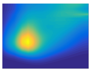
The footprints of these structures fill the whole channel, as shown in figure 6. Here, we have plotted the  $x$-average of the streamwise fluctuation, $\langle u\rangle _x$, as the background colour. The value of the vector field $(\langle v\rangle _x,\langle w\rangle _x)$ is represented with arrows. As we can see, it is possible to identify four structures with a width of $\ell _z \approx 6/8{\rm \pi} h$, approximately. This width is similar to the previous ones reported (Lee & Moser Reference Lee and Moser2018). The length of these structures can be obtained by studying the correlation in $x$ of $u$:
$u$:
 \begin{equation} R_x(s) = \frac{\langle u(x,y,z) u(x+s,y,z)\rangle}{u'^2},\quad R_z(s) = \frac{\langle u(x,y,z) u(x,y,z+s)\rangle}{u'^2}. \end{equation}
This correlation is shown at the channel centre, figure 7(a,b). The white lines mark the boundary among the rolls. Lee & Moser (Reference Lee and Moser2018) showed that for  ${{Re}}_\tau =500$, the structures were extremely long, with a length of at least $100h$. Alcántara-Ávila et al. (Reference Alcántara-Ávila, Barberá and Hoyas2019) obtained a similar result for thermal Couette flow. Our results offer a different trend than the previous results at smaller Reynolds numbers. In the C1000 case, the correlation is large for the four structures, filling the entire box length, while the structures of the C2000 case from $z/h=0$ to $3{\rm \pi}$ are smaller than the box. This can be appreciated better in figure 7(c). Here, the value of $R_x$ can be seen at $\ell _x =6{\rm \pi} h$. The maximum of this correlation is always greater than 0.3 for the C1000 case, but it is negative in some $z/h$ points for the C2000 case, indicating that the length of the coherent structure is less than $\ell_x$. Therefore, some parts of the channel can keep very large rolls, while in other regions, these rolls are limited to lengths below $\ell _x = 6{\rm \pi} h$. This is a new effect that has not been reported for turbulent Couette flow and points to the uncertainty that is observed for certain statistical quantities, such as the slope parameter $\psi$ in (3.1).
The  $x$-averaged field $\langle u\rangle _x$. The value of the vector field $(\langle v\rangle _x,\langle w\rangle _x)$ is represented with arrows. (a) C1000 case. (b) C2000 case.

(a,b)  $R_x(s)$ for C1000 (a) and C2000 (b). In both figures, we have added $\langle \phi \rangle _{x}$, showing the size in $z$ of the pair of rolls. (c) $R_x(s)$ at $\ell_x=6{\rm \pi} h$. The different rolls are marked using a dashed vertical line.

4. Conclusions
This paper presents two simulations at two different friction Reynolds numbers, namely 1000 and 2000. The simulations were carried out in a very large box of size  $L_x = 16{\rm \pi} h$, $L_y = 2 h$ and $L_z = 6{\rm \pi} h$. For the C2000 case, a clear log layer is only observed in parts. Through a fitting, a value of $\kappa = 0.397$ has been obtained. This value is a bit higher than Poiseuille channels and similar to other Couette ones. The scaling of the intensities is perfect in the buffer layer and below. The first maximum of $u'^+$ does not grow anymore, and a second maximum has clearly appeared at $y^+\approx 350$. This value is similar to that expected for Poiseuille channels (Hoyas et al. Reference Hoyas, Oberlack, Alcántara-Ávila, Kraheberger and Laux2022), but at a far lower Reynolds number. The scaling failure of the dissipation is also not present anymore. This can be traced to the constant value of $({{\rm d}}/{{\rm d}y})u'^+$ at the wall.
The intensities of the C2000 case are remarkably different from those at lower Reynolds numbers at the channel centre. This is probably due to the organization of the large scales of  $u$. These large scales were thought to be almost infinite. We obtained the same result for the C1000 case. However, for the C2000 case, some rolls present a finite size with a length of approximately $\ell _x = 6{\rm \pi}$. The width of every roll is approximately $\ell _z =6/8{\rm \pi}$. Simulations at a larger Reynolds number are needed to elucidate if these structures are bounded.
Funding
The authors gratefully acknowledge the provision of computing time on the Gauss Centre for Supercomputing e.V. on the GCS Supercomputer SuperMUC-NG at Leibniz Supercomputing Centre under project number pr92la. M.O. acknowledges partial funding by the German Research Foundation (DFG) under the project OB 96/48-1. S.H. is partially funded by project PID2021-128676OB-I00 by Ministerio de Ciencia, innovación y Universidades/FEDER.
Declaration of interests
The authors report no conflict of interest.


 Open access