


1. Introduction
Marine propellers shed large structures, especially from the tip of their blades and from their hub, having an important impact on their acoustic signature (Bagheri et al. Reference Bagheri, Seif, Mehdigholi and Yaakob2017; Cianferra, Petronio & Armenio Reference Cianferra, Petronio and Armenio2019; Wang, Göttsche & Abdel-Maksoud Reference Wang, Göttsche and Abdel-Maksoud2020; Ebrahimi et al. Reference Ebrahimi, Razaghian, Tootian and Seif2021; Razaghian et al. Reference Razaghian, Ebrahimi, Zahedi, Javanmardi and Seif2021; Petris, Cianferra & Armenio Reference Petris, Cianferra and Armenio2022; Posa et al. Reference Posa, Broglia, Felli, Cianferra and Armenio2022b) and affecting their interaction with downstream devices, such as rudders (Kinnas et al. Reference Kinnas, Lee, Gu and Natarajan2007; Felli, Camussi & Guj Reference Felli, Camussi and Guj2009; Felli & Falchi Reference Felli and Falchi2011; Felli, Grizzi & Falchi Reference Felli, Grizzi and Falchi2014; Badoe, Phillips & Turnock Reference Badoe, Phillips and Turnock2015; He & Kinnas Reference He and Kinnas2017; Villa et al. Reference Villa, Viviani, Tani, Gaggero, Bruzzone and Podenzana2018; Hu et al. Reference Hu, Zhang, Sun and Guo2019b, Reference Hu, Zhang, Guo, Sun, Chen and Guo2021; Wang et al. Reference Wang, Guo, Xu and Su2019; Villa, Franceschi & Viviani Reference Villa, Franceschi and Viviani2020; Felli Reference Felli2021; Posa & Broglia Reference Posa and Broglia2021, Reference Posa and Broglia2022a,Reference Posa and Brogliac,Reference Posa and Brogliad; Zhang et al. Reference Zhang, Li, Ma, Ning, Sun and Hu2022). A number of studies dealing with the wake of marine propellers are currently available in the literature, including both physical experiments and numerical simulations. However, the latter class of works often faces limitations in terms of accuracy of the approach, coming from modelling assumptions or the resolution of the computational grid.
Several Reynolds-averaged Navier–Stokes (RANS) computations on the subject were reported (see, for instance, Hong & Dong Reference Hong and Dong2010; Morgut & Nobile Reference Morgut and Nobile2012; Baek et al. Reference Baek, Yoon, Jung, Kim and Paik2015; Paik et al. Reference Paik, Hwang, Jung, Lee, Lee, Ahn and Van2015; Wang et al. Reference Wang, Guo, Su, Xu and Wu2017, Reference Wang, Guo, Su and Wu2018; Heydari & Sadat-Hosseini Reference Heydari and Sadat-Hosseini2020; Zhao, Zhao & Wan Reference Zhao, Zhao and Wan2020). Unfortunately, although RANS was demonstrated to be an appropriate tool for the prediction of the global performance of marine propellers, it is inherently not well suited to reproduce the instability mechanism typical of their wake, since turbulence is fully modelled, rather than resolved (Cai, Li & Liu Reference Cai, Li and Liu2019). Meanwhile, most turbulence models were developed on canonical, less challenging flow problems, so they are not specifically designed to represent the unsteady dynamics of the large tip and hub vortices shed by marine propellers and the properties of turbulence at their core. Detached-eddy simulation (DES) is aimed at improving the predictive capabilities of the computations, compared with RANS, since the large, energy-carrying structures of the flow are explicitly resolved away from walls. However, the RANS approach and its limitations are retained in the vicinity of the surface of the bodies immersed within the flow. Examples of this technique for the numerical prediction of the wake of marine propellers can be found in Muscari, Di Mascio & Verzicco (Reference Muscari, Di Mascio and Verzicco2013), Gong et al. (Reference Gong, Guo, Zhao, Wu and Song2018, Reference Gong, Guo, Phan-Thien and Khoo2020), Guilmineau et al. (Reference Guilmineau, Deng, Leroyer, Queutey, Visonneau and Wackers2018), Zhang & Jaiman (Reference Zhang and Jaiman2019), Sun et al. (Reference Sun, Wang, Guo, Zhang, Sun and Liu2020), Shi et al. (Reference Shi, Wang, Zhao and Zhang2022), Wang et al. (Reference Wang, Wu, Gong and Yang2021a, Reference Wang, Liu, Wang and Li2022b,Reference Wang, Liu, Wang and Lic) and Wang, Luo & Li (Reference Wang, Luo and Li2022e). In these studies, computational grids consisting of  $O(10^7)$ points are utilized, which is a significant step forward, in comparison with the typical resolutions adopted to conduct RANS computations, usually relying on meshes consisting of a few million points.
Large-eddy simulation (LES) is less often adopted in the field, due to its higher computational cost; LES computations need to be carried out using solvers with optimal conservation properties on computational grids able to explicitly resolve most energetic scales, limiting subgrid-scale (SGS) modelling to the smallest, dissipative scales only. These scales are more homogeneous and isotropic. As a result, for them the errors associated with modelling assumptions for turbulence are smaller. In recent years LES has become an increasingly popular tool for the simulation of marine propellers, thanks to the growing computing power of supercomputers. However, the LES studies currently available in the literature typically rely on computational grids consisting of  $O(10^7)$ points, similar to those for the DES computations reported above, and are usually targeted at analysing the process of instability of the wake system of marine propellers and the cavitation phenomena occurring within the large coherent structures they shed (Liefvendahl Reference Liefvendahl2010; Liefvendahl, Felli & Troëng Reference Liefvendahl, Felli and Troëng2010; Asnaghi, Svennberg & Bensow Reference Asnaghi, Svennberg and Bensow2018a,Reference Asnaghi, Svennberg and Bensowb, Reference Asnaghi, Svennberg and Bensow2020a; Hu et al. Reference Hu, Wang, Zhang, Chang and Zhao2019a; Zhu & Gao Reference Zhu and Gao2019; Ahmed, Croaker & Doolan Reference Ahmed, Croaker and Doolan2020; Asnaghi et al. Reference Asnaghi, Svennberg, Gustafsson and Bensow2020b; Long et al. Reference Long, Han, Ji, Long and Wang2020; Kimmerl, Mertes & Abdel-Maksoud Reference Kimmerl, Mertes and Abdel-Maksoud2021a,Reference Kimmerl, Mertes and Abdel-Maksoudb; Wang et al. Reference Wang, Wu, Gong and Yang2021b, Reference Wang, Li, Guo, Wang and Sun2022a; Wang, Liu & Wu Reference Wang, Liu and Wu2022d). However, the resolution of the computational grid and in turn the range of scales that LES is able to explicitly resolve to accurately reproduce the mechanism of wake instability has been pushed even forward in the works by Balaras, Schroeder & Posa (Reference Balaras, Schroeder and Posa2015), Kumar & Mahesh (Reference Kumar and Mahesh2017), Posa et al. (Reference Posa, Broglia, Felli, Falchi and Balaras2019), Posa, Broglia & Balaras (Reference Posa, Broglia and Balaras2022a) and Posa (Reference Posa2022b).
Kumar & Mahesh (Reference Kumar and Mahesh2017) adopted an unstructured grid consisting of 181 million hexahedral cells to conduct wall-resolved computations and analyse in detail the development and eventual instability of the wake shed by the five-bladed DTMB 4381 propeller at the design working condition, using a body-fitted approach. Their state-of-the-art computations revealed that the onset of the instability of the tip vortices was attributable to their interaction with the smaller vortices arising from the roll-up by the thin wakes shed from the trailing edge of the propeller blades. An immersed-boundary (IB) technique was instead adopted by Balaras et al. (Reference Balaras, Schroeder and Posa2015), Posa et al. (Reference Posa, Broglia, Felli, Falchi and Balaras2019, Reference Posa, Broglia and Balaras2022a) and Posa (Reference Posa2022b). Balaras et al. (Reference Balaras, Schroeder and Posa2015) studied the seven-bladed INSEAN E1619 propeller, using a cylindrical grid consisting of more than 3 billion points. Their computations demonstrated the ability of the overall LES/IB approach in reproducing the process of instability of the tip vortices at both design and heavy-loaded conditions, developing according to the mechanisms discussed in the theoretical work by Widnall (Reference Widnall1972) and observed in the physical experiments by Felli, Camussi & Di Felice (Reference Felli, Camussi and Di Felice2011). A cylindrical grid of 840 million points was adopted by Posa et al. (Reference Posa, Broglia, Felli, Falchi and Balaras2019) to reproduce the wake generated by the seven-bladed INSEAN E1658 propeller across three values of advance coefficient, reporting detailed comparisons with the particle imaging velocimetry (PIV) measurements by Felli & Falchi (Reference Felli and Falchi2018) and demonstrating a very close agreement with them. The same propeller was simulated by Posa et al. (Reference Posa, Broglia and Balaras2022a), using a finer computational grid consisting of 3.8 billion points. A detailed vortex core analysis was reported for both tip and hub vortices. Both studies by Posa et al. (Reference Posa, Broglia, Felli, Falchi and Balaras2019, Reference Posa, Broglia and Balaras2022a) revealed the importance of the interaction between the tip vortices and the wake shed by the following blades in promoting the instability of the former, accelerated at higher rotational speeds by their decreasing pitch, shifting the streamwise location of this interaction closer to the propeller plane. More recently, Posa (Reference Posa2022b) utilized a grid of 5 billion points to simulate both conventional and tip-loaded propellers at design working conditions, to compare the development of their wakes and in particular their tip vortices. The LES computations revealed that, despite the use of pressure side winglets at the end of the tip-loaded blades, splitting the tip vortices into two smaller helical structures, tip loading still resulted in more intense tip vortices, in comparison with the conventional blade design.
Although all LES studies above provided important information on the wake dynamics of marine propellers, several details on the properties of turbulence and their evolution during the instability of the tip and hub vortices are still missing. They are required, since they could serve as a reference for lower-fidelity approaches, relying on more conventional strategies of turbulence modelling, such as RANS, to verify their predictive capabilities and their deviations from the actual behaviour of turbulence. Information on the properties of turbulence is especially needed at the core of the tip and hub vortices, where conventional modelling is challenged the most. In contrast, studies targeted at the vortex core analysis are quite limited in the literature. In other words, data from high-fidelity computations could be useful to tune turbulence models, with the purpose of improving their accuracy in this particular class of flows. Taken into account the limited access to supercomputing resources, this achievement is important to make the computational study of propellers more affordable to a wider community of scientists and engineers, by decreasing the computational cost of the simulation of their fluid dynamics.
In the present study, results from LES simulations, conducted on a computational grid consisting of approximately 5 billion points, are exploited to gain insight into the properties of turbulence at the core of the tip and hub vortices shed by a marine propeller. This work is the extension of an earlier study (Posa Reference Posa2022a), focused on the analysis of the dependence of the intensity of the tip and hub vortices on the working conditions of the propeller. While vorticity at their core was found almost proportional to the rotational speed of the propeller, the growth of both turbulence maxima and pressure minima, which are potential sources of cavitation phenomena, was verified to be faster than linear. In addition, in the earlier work by Posa (Reference Posa2022b) the wake development of the same tip-loaded propeller, including a downstream shaft, was compared against that of a conventional propeller without winglets, to assess the ability of winglets of reducing the intensity of the tip vortices, despite the higher load at the outer radii of the propeller blades.
In this study, the anisotropy of turbulence at the core of the tip and hub vortices is analysed as a function of both the streamwise coordinate downstream of the propeller and its load conditions. Furthermore, its deviation from the assumption of Boussinesq's hypothesis of proportionality between the deformation tensor and the deviatoric part of the Reynolds stresses is explored. Despite the importance of the subject, the literature on the anisotropy of turbulence within vortices is rather limited, due to the challenge of performing a vortex core analysis through both experiments and computations.
Hot-wire probes were utilized to perform measurements at the core of a vortex by Phillips & Graham (Reference Phillips and Graham1984). The vortex was coaxial with a jet or a wake in their experiments. These conditions were found to accelerate the radial dispersion of vorticity, by producing higher levels of Reynolds stresses. However, in the wake flow the Reynolds stresses were found to be an order of magnitude lower than in the jet flow, in agreement with the slower rate of decay of the tangential velocity within the vortex. The results by Phillips & Graham (Reference Phillips and Graham1984) did not show strong levels of anisotropy of turbulence at the core of the vortex, with similar tangential and radial stresses and only slightly lower axial stresses.
Moore et al. (Reference Moore, Moore, Heckel and Ballesteros1994) analysed the turbulence within the tip leakage vortex generated by a linear turbine cascade on a plane located just upstream of the trailing edge of the cascade, by using data from hot-wire measurements. Turbulence was found to be almost isotropic in the region between the core of the tip leakage vortex and the endwall separation. Anisotropy developed away from there, due to the shear between the vortex and the free stream as well as to the flow recirculating from the tip leakage vortex towards the suction side of the blades composing the cascade. In other words, the study by Moore et al. (Reference Moore, Moore, Heckel and Ballesteros1994) found the most significant contributions to anisotropy of turbulence originating from the interaction of the tip leakage vortex with the surrounding flow and walls, rather than from phenomena occurring at the core of the vortex itself. A more recent study on a similar subject was reported by Li, Chen & Katz (Reference Li, Chen and Katz2019). They conducted experiments in the optical refractive index-matched facility of the Johns Hopkins University, dealing with the blade tip region of two water jet pumps and an aviation compressor, focusing their analysis on the region populated by the tip leakage vortex. Interestingly, they reported that the distribution of the Reynolds stresses, although extremely anisotropic, was similar across different geometries. They also verified the lack of correlation between the Reynolds stresses and mean strain rates, resulting in a complex distribution of both positive and negative values of turbulent viscosity. However, also for the turbulent viscosity, similar patterns were observed across different turbomachinery geometries.
Chow, Zilliac & Bradshaw (Reference Chow, Zilliac and Bradshaw1997a,Reference Chow, Zilliac and Bradshawb) studied the anisotropy of turbulence within the vortex shed from the tip of a wing by using triple-wire probe measurements. Also in this case a lag of the Reynolds stresses, relative to the strain rate tensor, was observed. In the cylindrical frame of reference centred at the core of the vortex, the radial turbulent stresses were found to be higher than the tangential ones. These results were verified in a later study by Ramasamy et al. (Reference Ramasamy, Johnson, Huismann and Leishman2007, Reference Ramasamy, Johnson, Huismann and Leishman2009), who performed PIV measurements at the core of the vortex shed from the tip of a rotor. However, they reported the stresses in the axial direction to be the highest. The turbulent stresses within the vortex shed from the tip of a wing were also studied by Churchfield & Blaisdell (Reference Churchfield and Blaisdell2009), who utilized the experimental data by Chow et al. (Reference Chow, Zilliac and Bradshaw1997a,Reference Chow, Zilliac and Bradshawb) to verify the accuracy of a number of turbulence models. In particular, they found the best performance by the Spalart–Allmaras model with a curvature correction (Spalart & Shur Reference Spalart and Shur1997), while both the standard Spalart–Allmaras (Spalart & Allmaras Reference Spalart and Allmaras1994) and Menter shear stress transport (Menter Reference Menter1994) models overpredicted the Reynolds stresses. Churchfield & Blaisdell (Reference Churchfield and Blaisdell2009) concluded also that, although the Rumsey–Gatski  $\kappa$– $\epsilon$ ( $\kappa$, turbulent kinetic energy; $\epsilon$, turbulent dissipation) algebraic Reynolds stress model (Rumsey & Gatski Reference Rumsey and Gatski2001) was not the best performing, it was the only one to properly predict some lag of the tensor of the Reynolds stresses, relative to the deformation tensor. They reported a resolution of their computational grid within the vortex core of 21 grid points. In the same line, Skinner, Green & Zare-Behtash (Reference Skinner, Green and Zare-Behtash2020) recently conducted stereo PIV on the vortex shed by a swept-tapered planar wing, representative of the flow structures shed by typical mid-sized commercial aircraft wings. Their study revealed relaminarization at the vortex core for all investigated angles of attack. They also reported a four-lobed topology for both Reynolds stresses and strain rates, but characterized by different orientations. However, this comparison was limited to only one component of the two tensors.
The anisotropy of turbulence at the core of the sonar dome tip vortex generated by a surface combatant ship in static drift was studied by Visonneau, Guilmineau & Rubino (Reference Visonneau, Guilmineau and Rubino2018, Reference Visonneau, Guilmineau and Rubino2020) by means of DES computations and experiments. At the onset of the vortex, significant deviations from isotropy were found, which explained the poor predictions by RANS computations. The experiments revealed an axisymmetric ‘cigar-shaped’, rod-like state, characterized by the lead of one component of the velocity fluctuations over the other two components. As the vortex developed away from the wall of the ship, turbulence at its core was found to approach gradually a more isotropic state. The comparison between DES and experiments was good, although at the onset of the vortex DES predicted, in contrast with the experiments, turbulence spanning a wider range of anisotropic conditions, including two-component turbulence and a ‘pancake-shaped’, disk-like axisymmetric state, characterized by one component of the turbulent fluctuations of velocity being smaller than the others.
Although all studies reported above provided a remarkable insight into the anisotropy of turbulence at the core of the vortices shed by wings, rotors, ships or even in turbomachinery devices, a detailed discussion of its properties within the tip and hub vortices shed by propellers is missing. Meanwhile, the same studies suggested that the anisotropy of turbulence at the core of vortices is significantly affected by the particular features of their generators. This is problematic if turbulence models need to be tuned to properly handle this class of flows by exploiting data available through high-fidelity computations or experiments.
The results of the present study will show the development of a ‘cigar-shaped’ axisymmetric turbulence at the core of the tip vortices shed by a marine propeller, as their instability develops. Then, the break-up of the tip vortices results in turbulence shifting again towards a more isotropic state. In contrast, during instability the hub vortex will show the development of a ‘pancake-shaped’ axisymmetric turbulence, characterized by larger turbulent fluctuations of the radial and azimuthal velocities, in comparison with those affecting the axial velocity. However, also for the hub vortex the faster instability at higher loads results in a faster recovery of a isotropic state of turbulence.
The present paper is organized as follows. In § 2, the LES methodology, coupled with an IB technique, is introduced, providing also information about the approach adopted for the numerical solution of the problem. In § 3, the numerical set-up of the simulations is presented, including details on the flow problem and the resolutions adopted in both space and time. In § 4, the results of the LES computations are analysed, dealing with the anisotropy of turbulence at the core of the tip and hub vortices shed by a marine propeller, its deviations from Boussinesq's hypothesis for turbulence and comparisons between resolved and modelled Reynolds stresses, demonstrating that the present computations were able to resolve most of the turbulence. Finally, the conclusions of this study are summarized in § 5.
2. Methodology
The filtered Navier–Stokes equations (NSEs) for incompressible flows were resolved in non-dimensional form
 $$\begin{gather}
\frac{\partial u_i}{\partial x_i} = 0,\quad i=1,2,3,
\end{gather}$$
$$\begin{gather}
\frac{\partial u_i}{\partial x_i} = 0,\quad i=1,2,3,
\end{gather}$$ $$\begin{gather}\frac{\partial
u_i}{\partial t} + \frac{\partial u_i u_j}{\partial x_j }
={-} \frac{\partial p}{\partial x_i} - \frac{\partial
\tau_{ij}}{\partial x_j} + \frac{1}{Re}
\frac{\partial^2 u_i}{\partial x_j^2} + f_i,\quad
i,j=1,2,3,
\end{gather}$$
$$\begin{gather}\frac{\partial
u_i}{\partial t} + \frac{\partial u_i u_j}{\partial x_j }
={-} \frac{\partial p}{\partial x_i} - \frac{\partial
\tau_{ij}}{\partial x_j} + \frac{1}{Re}
\frac{\partial^2 u_i}{\partial x_j^2} + f_i,\quad
i,j=1,2,3,
\end{gather}$$
where  $t$ is time, $x_i$ the coordinate in space along the direction $i$,
$i$,  $u_i$ the component in the same direction of the filtered velocity vector, $p$ the filtered pressure and $\tau_{ij}$ the SGS stress tensor. Scaling the dimensional equations results in the non-dimensional Reynolds number, $Re=UL/\nu$, where $U$ is the reference velocity scale, $L$ the reference length scale and $\nu$ the kinematic viscosity of the fluid.
The NSEs were filtered, which means that only the large, energy-carrying structures of the flow were resolved, while the smallest, dissipative scales were modelled using a SGS model. Practically, when the NSEs are numerically resolved, the size of the filter is defined by the local resolution of the computational grid utilized to discretize the domain. Filtering the NSEs results in an additional term, the SGS stress tensor,  $\tau _{ij}$, coming from the convective terms of the original equations. This tensor represents the action of the smallest, unresolved scales on the largest, resolved ones. In the present study it was modelled using the wall adaptive local eddy-viscosity model, developed by Nicoud & Ducros (Reference Nicoud and Ducros1999), which was already successfully utilized in a number of studies dealing with marine propellers, also in the framework of the present solver (Posa, Broglia & Balaras Reference Posa, Broglia and Balaras2020a,Reference Posa, Broglia and Balarasb, Reference Posa, Broglia and Balaras2021; Posa & Broglia Reference Posa and Broglia2022b). It utilizes the square of the velocity gradient tensor of the resolved field to reconstruct the unresolved stresses. This way, it is able to account for both regions of large strain and rotation within the flow. More details on the WALE model can be found in the work by Nicoud & Ducros (Reference Nicoud and Ducros1999).
The last term in (2.2),  $f_i$, was utilized in the framework of an IB methodology to enforce the no-slip condition on the surface of the bodies immersed within the flow. In IB methods the computational domain is discretized by means of a regular, Eulerian grid, where the NSEs are resolved. This grid is not required to fit the bodies immersed within the flow. They are represented by means of Lagrangian grids, which are ‘immersed’ within the Eulerian grid and free to move across its cells. These Lagrangian grids allow separation of the Eulerian points into ‘solid’, ‘fluid’ and ‘interface’. The interface points are those placed at the boundary between the solid and fluid regions of the computational domain. The boundary conditions are enforced by means of $f_i$ at the solid and interface points. At the solid points, $f_i$ is computed as the value of the forcing term which results in a velocity condition corresponding to the velocity of the body. At the interface points, the velocity condition enforced through $f_i$ comes from a linear reconstruction of the solution between the no-slip requirement on the surface of the Lagrangian grid and the solution at the fluid points in the vicinity of the particular interface point. The IB methods are well-established techniques utilized for the solution of fluid dynamic problems involving complex geometries. For more details on the particular implementation utilized in the framework of this study, the reader is referred to the work by Yang & Balaras (Reference Yang and Balaras2006).
The NSEs were numerically resolved on a staggered, cylindrical grid, using second-order, central finite differences. As discussed in detail by Fukagata & Kasagi (Reference Fukagata and Kasagi2002), this strategy achieves optimal conservation properties for the discretized version of the NSEs, that is the exact conservation of mass, momentum and kinetic energy. The advancement of the solution in time utilized a fractional-step technique (Van Kan Reference Van Kan1986). For the discretization in time of the convective, viscous and SGS terms of the momentum equation the explicit, three-step Runge–Kutta scheme was adopted. However, for efficiency of the solution, in the regions of the highest resolution in space the implicit Crank–Nicolson scheme was exploited. This was the case of the terms of azimuthal derivatives in the vicinity of the axis of the cylindrical grid and those of radial derivatives at the coordinates close to the tip of the propeller blades. Although the angular spacing of the cylindrical grid was uniform, its linear, azimuthal spacing was a function of the radial coordinate, going to zero towards the grid axis. The radial grid was refined at the tip of the propeller blades to properly resolve the helical vortices they shed. The Poisson problem arising from the continuity requirement was resolved by using trigonometric transformations along the azimuthal direction, splitting the hepta-diagonal system of equations into a series of penta-diagonal systems. Each of them was inverted using an efficient direct solver (Rossi & Toivanen Reference Rossi and Toivanen1999). The same, LES/IB NSE solver was already successfully adopted in a number of studies dealing with marine propellers, including also validations against physical experiments (Balaras et al. Reference Balaras, Schroeder and Posa2015; Posa et al. Reference Posa, Broglia, Felli, Falchi and Balaras2019, Reference Posa, Broglia and Balaras2022a; Posa Reference Posa2022b). More details on the overall methodology can be found in the works by Balaras (Reference Balaras2004) and Yang & Balaras (Reference Yang and Balaras2006).
3. Computational set-up
The present study deals with the tip-loaded propeller with pressure side winglets illustrated in figure 1, which was designed at the Naval Surface Warfare Center (Carderock Division) of the US Navy by Brown et al. (Reference Brown, Sánchez-Caja, Adalid, Black, Pérez-Sobrino, Duerr, Schroeder and Saisto2014). It was simulated in open-water conditions, which means that the propeller works in isolated conditions within a uniform flow. This is the same configuration for which Brown et al. (Reference Brown, Sánchez-Caja, Adalid, Black, Pérez-Sobrino, Duerr, Schroeder and Saisto2014) reported experimental results on the global parameters of performance, adopted here for validation purposes. It is also worth noting that, in the present computations, the geometry was simulated with no downstream shaft, to allow the generation of a large hub vortex in the propeller wake. This was one of the major subjects of the analysis reported in this study, together with the vortices shed from the tip of the propeller blades. The downstream shaft was obviously required in the physical experiments conducted by Brown et al. (Reference Brown, Sánchez-Caja, Adalid, Black, Pérez-Sobrino, Duerr, Schroeder and Saisto2014) for supporting and rotating the propeller during their open-water tests. However, marine propellers work in push-type configuration, with no downstream shaft. Therefore, removing the shaft from the computational set-up allows the present simulations to reproduce more realistic working conditions, which are also characterized by the formation of a hub vortex in the wake of the propeller. This was not allowed in the experimental set-up considered by Brown et al. (Reference Brown, Sánchez-Caja, Adalid, Black, Pérez-Sobrino, Duerr, Schroeder and Saisto2014). However, in the framework of this study, LES computations were also conducted on the geometry including the downstream shaft and the effect on the anisotropy of the turbulence at the core of the tip vortices is illustrated in § 4.7.

Figure 1. Visualizations of the propeller geometry.
Brown et al. (Reference Brown, Sánchez-Caja, Adalid, Black, Pérez-Sobrino, Duerr, Schroeder and Saisto2014) performed both physical experiments and RANS computations across a range of working conditions, to reconstruct the characteristic curves of propeller performance. The working conditions of marine propellers are characterized by means of the advance coefficient, which is the typical quantity expressing their rotational speed in non-dimensional form. It is defined as  $J=V/nD$, where $V$ is the advance velocity, $n$ the frequency of the propeller rotation and $D$ its diameter. Since open-water conditions are considered, the advance velocity is equal to the free-stream velocity, $U_\infty$. The design advance coefficient for the particular propeller is equal to $J=0.923$. This case was simulated in the framework of the present study and will be denoted as J0 hereafter. Four additional working conditions were computed, moving towards lower values of advance coefficient: $J=0.8$ (J1), $J=0.7$ (J2), $J=0.6$ (J3) and $J=0.5$ (J4). It should be noted that decreasing the advance coefficient is equivalent to increasing the rotational speed, corresponding to growing loads and to more intense tip and hub vortices shed by the propeller.
In the field of marine propellers the Reynolds number is typically defined assuming as reference the chord of the propeller blades at  $70\,\%R$, where $R=D/2$ is the radial extent of the propeller, and the relative velocity of the flow at the same radial location. The definition of the Reynolds number is
 \begin{equation} Re_p = \frac{c(70\,\%R) \sqrt{V^2 + (0.7\ 2 {\rm \pi}n R)^2}}{\nu}, \end{equation}
where  $c$ is the chord of the propeller blades, which is a function of the radial coordinate, and $\nu$ is the kinematic viscosity of water. Brown et al. (Reference Brown, Sánchez-Caja, Adalid, Black, Pérez-Sobrino, Duerr, Schroeder and Saisto2014) performed experiments and computations at model-scale Reynolds numbers of $O(10^5)$. The present simulations were carried out in the same conditions. In particular, the values of Reynolds number corresponding to the five simulated advance coefficients range from $Re_p \approx 430,000$ at J0 to $Re_p \approx 750\,000$ at J4, since decreasing advance coefficients are equivalent to increasing velocities.
All computations were conducted within a cylindrical domain (figure 2) of radial extent equivalent to  $5.0D$, centred at the axis of the propeller. Its inflow and outflow sections were placed $2.5D$ upstream and $5.0D$ downstream of the propeller plane, respectively. For clarity of the following discussion, it is worth noting that the origin of the radial coordinates is located on the propeller axis, and that of the axial coordinates on the propeller plane. They are oriented outwards and downstream, respectively. The azimuthal coordinates are oriented in the counter-clockwise direction, looking from downstream. To mimic open-water conditions a uniform axial velocity, equal to $U_\infty$, was enforced at the inlet section, while convective conditions were prescribed at the outlet section for all velocity components, using $U_\infty$ as the convective velocity. At the lateral, cylindrical boundary of the domain, homogeneous Neumann conditions for velocity allowed reproduction of free-stream conditions. At all (inlet, outlet and lateral) boundaries of the computational domain, homogeneous Neumann conditions were prescribed for both pressure and eddy viscosity. For all variables, periodic conditions were utilized at the azimuthal boundaries. The no-slip requirement on the surface of the propeller was prescribed by means of the IB technique discussed in § 2.

Figure 2. Propeller model (yellow) within the computational domain (cyan).
The computational domain was discretized by using a cylindrical, Eulerian grid, consisting of an overall number of  $1192 \times 2050 \times 2050$ points along the radial, azimuthal and axial directions, respectively. Cross-stream and meridian slices of this grid are shown in figures 3 and 4, where only a small sample of points is represented, for visibility of the grid lines (1 point of every 256 on both slices). The use of a regular grid was allowed by the IB technique. The cylindrical topology was preferred to the Cartesian one, since it allowed clustering of Eulerian points in the region of interest of the domain, at inner radial coordinates, where the propeller and its wake are placed, since the linear, azimuthal spacing of the grid becomes finer towards its axis, even using a constant angular spacing. The radial and axial grids were also refined in the vicinity of the propeller and in its wake. In particular, the radial grid reaches its minimum spacing at the tip of the propeller blades ( ${\rm \Delta} r/D = 4 \times 10^{-4}$ at $r/D=0.5$), with the purpose of resolving the tip vortices and their downstream development and instability, as demonstrated by the following discussion on the wake features. Also, the axial grid achieves its minimum spacing across the propeller blades ( ${\rm \Delta} z/D = 5 \times 10^{-4}$ at $z/D=0.0$) and is smoothly stretched downstream, up to $z/D \approx 3.5$, again to properly capture the development of instability phenomena. Some details on the distribution of the grid points are illustrated in figures 3 and 4. In particular, it was verified from the present computations that the adopted Eulerian grid was able to achieve, on average, levels of resolution corresponding to 4, 25 and 12 wall units across the normal, streamwise and spanwise directions, respectively, relative to the surface of the propeller blades. This resolution can be considered adequate for wall-resolved LES, based on the criteria reported in the literature (Georgiadis, Rizzetta & Fureby Reference Georgiadis, Rizzetta and Fureby2010). The following discussion of the results in § 4.5 will also demonstrate that the modelled stresses are two orders of magnitude lower than the resolved ones, even at the core of the tip and hub vortices, giving confidence about the accuracy of the computations and their ability in resolving all important, energy-carrying scales of the flow.

Figure 3. Cross-stream slice of the cylindrical grid. For visibility, only 1 of every 256 points is shown.

Figure 4. Meridian slice of the cylindrical grid. For visibility, only 1 of every 256 points is shown.
Although it is necessary to acknowledge that a sensitivity study on the level of resolution of the computational grid was not carried out in the present case, due to limitations of computational resources, the adopted resolution was selected based on the author's experience of the LES simulation of marine propellers. For instance, in the work by Balaras et al. (Reference Balaras, Schroeder and Posa2015), the seven-bladed, submarine INSEAN E1619 propeller was simulated, adopting two computational grids consisting of 840 million and 3.3 billion points, respectively, finding in both cases a close agreement with measurements on global parameters of performance. In a later study (Posa et al. Reference Posa, Broglia, Felli, Falchi and Balaras2019), a grid consisting of 840 million points was utilized to analyse the performance and wake development of the INSEAN E1658 propeller, including also successful comparisons against dynamometric measurements on thrust and torque and PIV experiments on the wake topology by Felli & Falchi (Reference Felli and Falchi2018). It is worth noting that this grid was coarser than the one adopted for the present study across all directions in space, consisting of an overall number of points six times smaller. Nonetheless, the agreement with the flow fields measurements by Felli & Falchi (Reference Felli and Falchi2018) was found to be very satisfactory, also in terms of the ability of the simulations in capturing the tip vortices shed by the INSEAN E1658 propeller. In a later study (Posa et al. Reference Posa, Broglia and Balaras2022a), a finer grid of 3.8 billion points was adopted for the same flow problem, to analyse in more detail the development of the tip and hub vortices. The comparison with the experiments by Felli & Falchi (Reference Felli and Falchi2018) was almost unchanged, relative to the one reported on the coarser grid considered by Posa et al. (Reference Posa, Broglia, Felli, Falchi and Balaras2019). Therefore, the present grid was designed, based on that utilized by Posa et al. (Reference Posa, Broglia and Balaras2022a), with the purpose of increasing its resolution across the span of the propeller blades and especially at their tip, to take into account the presence of end plates.
In the framework of the adopted IB methodology, the geometry of the propeller was represented by using a Lagrangian grid, discretizing its surface by means of  $106\,000$ triangular elements and ‘immersed’ within the Eulerian grid. A visualization of this Lagrangian grid is provided in figure 5. It is shown that the regions of the highest curvature of the propeller geometry are characterized by the finest refinement of the Lagrangian grid, which is achieved at the tip of the propeller blades and their pressure side winglets.

Figure 5. Details of the Lagrangian grid of the propeller: (a) upstream, (b) lateral, (c) downstream and (d) isometric views.
The resolution in time of all computations was prescribed by the stability restrictions coming from the explicit discretization of the convective terms of the momentum equation. During all simulations a constant value of the Courant–Friedrichs–Lewy number equal to 1 was enforced, to meet the stability requirements of the three-step Runge–Kutta scheme. On average, 6800 steps of advancement of the numerical solution in time were required for the propeller to perform a full revolution. Each case was advanced during two flow-through times to develop the wake flow, starting from uniform axial velocity conditions. Then, for each case, statistics were computed at run time during 10 additional revolutions. By using this strategy, all instantaneous realizations of the solution were included within the statistical sample, which allowed maximizing of its size. Statistics were computed as phase averages on a grid rotating together with the propeller. This way, they were able to isolate the coherent structures shed by the propeller, in particular its tip and hub vortices, as long as they remained synchronized with its rotation, before wake instability led to large-scale deviations. In the following, the phase average of any quantity  $f$ will be indicated as $\hat {f}$, and the phase-averaged root-mean-squares of their fluctuations as $\widehat {f'}$. In particular, these statistics will be reported for the three velocity components along the radial, azimuthal and axial directions of the cylindrical reference frame centred at the intersection between the propeller plane and its axis. They will be denoted as $u$,
$u$,  $v$ and $w$, respectively. Therefore, the corresponding phase-averaged normal Reynolds stresses will be indicated below as $\widehat {u'u'}$, $\widehat {v'v'}$ and $\widehat {w'w'}$.
All simulations were carried out by means of an in-house parallel Fortran solver, exploiting high performance computing. The overall flow problem was split across 2048 cores of distributed-memory clusters, decomposing the cylindrical grid into cylindrical subdomains. Communications between them were handled by means of calls to message passing interface libraries. Most computations were performed on MareNostrum4 at the Barcelona Supercomputing Center in Spain, in the framework of a PRACE (Partnership for Advanced Computing in Europe) project. This cluster was equipped with 2 ${\times}$Intel Xeon Platinum 8160 24C processors, working at 2.1 GHz, with a total of 48 cores per node. Each computing node was equipped with 96 GB of main memory. The physical time required by each step of advancement of the solution was equal to approximately 22 seconds. This resulted in a physical time of approximately 900 hours required to simulate each working condition of the propeller. Therefore, the computational cost of each case was equivalent to approximately 2 million core hours. Due to the large size of the data to be analysed and the resulting memory requirements, post-processing activities were also conducted on the same cluster by using in-house-developed parallel Fortran codes, splitting again the whole problem across 2048 cores. Parallel I/O activities were handled by calls to HDF5 (Hierarchical Data Format version 5) libraries. However, the computational cost of post-processing amounted to only a few per cent of that of the main production runs. Most visualizations reported in this manuscript exploited the parallel capabilities of Paraview software.
4. Results
4.1. Global performance and comparison with experiments
The performance of marine propellers is characterized through the thrust and torque coefficients and the resulting efficiency of propulsion, defined as
 \begin{equation} K_T = \frac{T}{\rho n^2 D^4},\quad K_Q = \frac{Q}{\rho n^2 D^5},\quad \eta = \frac{J K_T}{2{\rm \pi} K_Q}, \end{equation}
where  $T$ is the axial force generated by the propeller, while $Q$ is the moment required for its rotation. Comparisons between the results of the present computations and the experiments by Brown et al. (Reference Brown, Sánchez-Caja, Adalid, Black, Pérez-Sobrino, Duerr, Schroeder and Saisto2014) are reported as time averages in figure 6, where the vertical dashed line indicates the design working condition. In each panel of figure 6 the right vertical scale deals with the error of the LES compared with the reference experiments. The agreement was verified to be very satisfactory. On the thrust coefficient (figure 6a) the error keeps within $2\,\%$. On the torque coefficient (figure 6b) it is only slightly higher than $2\,\%$ at the design working condition. For the efficiency of propulsion the error is equal to approximately $4\,\%$ at the design advance coefficient, moving towards smaller values at higher loads, as shown in figure 6(c). Both the experiments by Brown et al. (Reference Brown, Sánchez-Caja, Adalid, Black, Pérez-Sobrino, Duerr, Schroeder and Saisto2014) and the present computations show that, for increasing loads (decreasing advance coefficients), both thrust and torque experience an increase, which is faster for the latter, resulting in decreasing values of efficiency of propulsion.

Figure 6. Comparison between the experiments by Brown et al. (Reference Brown, Sánchez-Caja, Adalid, Black, Pérez-Sobrino, Duerr, Schroeder and Saisto2014) and the present LES computations: time-averaged values of (a)  $K_T$, (b) $10K_Q$ and (c) $\eta$. The right vertical scale for the relative error of LES against the experiments. The dashed vertical line for the design working condition.
Brown et al. (Reference Brown, Sánchez-Caja, Adalid, Black, Pérez-Sobrino, Duerr, Schroeder and Saisto2014) did not perform flow field measurements in the wake. However, they conducted cavitation tunnel visualizations of the tip vortices. From them, Brown, Schroeder & Balaras (Reference Brown, Schroeder and Balaras2015) were able to provide information on the final contraction ratio of the tip vortices,  $R_c=r_c/R$, which is the ratio between the final radial coordinate of the tip vortices at the end of the initial wake contraction, $r_c$, due to acceleration of the flow through the propeller plane, and the radial extent of the propeller, $R$. In addition, they provided the helical pitch angle of the tip vortices, $\beta$, which is their angle relative to the azimuthal direction. Their values are available for the experiments conducted at the nominal working condition only. The definitions of $R_c$ and $\beta$ are reported in figure 7, where the signature of the tip vortices is isolated in the flow fields generated by the present LES computations by means of time-averaged and phase-averaged contours of vorticity magnitude in (a,b), respectively. Brown et al. (Reference Brown, Schroeder and Balaras2015) reported values of $R_c=0.90$ and ${\beta =21.5^{\circ }}$. In the present simulations at the same working condition, J0, the final contraction ratio and the helical pitch angle were equal to $R_c=0.89$ and $\beta =22.0^{\circ }$, respectively.

Figure 7. (a) Contours of time-averaged vorticity magnitude on a meridian plane: definition of the final contraction ratio,  $R_c$. (b) Contours of phase-averaged vorticity magnitude on a cylindrical slice of the computational grid: definition of the helical pitch angle, $\beta$. Vorticity values scaled by $U_\infty /D$. Flow fields from the LES computation at the design working condition, J0.
4.2. Wake topology
An overview of the wake topology is provided in this section. Figure 8 shows isosurfaces of pressure coefficient from instantaneous realizations of the solution, coloured by vorticity magnitude. The pressure coefficient was defined as  $c_p=(p-p_\infty )/(0.5 \rho U_\infty ^2)$, where $p_\infty$ and $U_\infty$ are the free-stream pressure and velocity, respectively, while $\rho$ is the density of the fluid. Regions of minima of the pressure coefficient,
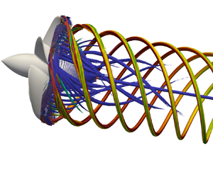
  $c_p$, were utilized to identify the major vortices shed by the propeller, as three-dimensional isosurfaces, which are the helical tip vortices at the outer boundary of its wake and the hub vortex at its axis. It is worth noting that their intensity is a function of the advance coefficient. Therefore, the isosurfaces in figure 8 refer to growing minima of pressure coefficient for lower values of the advance coefficient. Also the colour scale for vorticity changes across panels.

Figure 8. Isosurfaces of pressure coefficient,  $c_p$, from instantaneous realizations of the solution, coloured by vorticity magnitude (scaled by $U_\infty /D$). Comparison across advance coefficients: (a) J0 ( $c_p=-0.4$); (b) J1 ( $c_p=-0.6$); (c) J2 ( $c_p=-0.8$); (d) J3 ( $c_p=-1.2$); (e) J4 ( $c_p=-1.6$). Note that both the colour scale of the contours and the $c_p$ value utilized to generate the isosurfaces change across panels.
The visualizations in figure 8 demonstrate the ability of the computations in capturing the instability of the tip vortices. It is interesting to see that increasing load conditions result in an upward shift of this instability, which moves closer to the propeller plane. This is mainly the result of smaller values of the pitch of the helix of the tip vortices: smaller relative distances between tip vortices cause faster mutual inductance phenomena, promoting their faster destabilization and break-up, as illustrated in the visualizations from the experimental studies on the wake of marine propellers conducted by Felli, Guj & Camussi (Reference Felli, Guj and Camussi2008) and Felli et al. (Reference Felli, Camussi and Di Felice2011). This physics is shown also by means of isosurfaces of the second invariant of the velocity gradient tensor (the  $\mathcal {Q}$-criterion proposed by Jeong & Hussain Reference Jeong and Hussain1995) in figure 9 from phase-averaged statistics of the flow. The signature of the tip vortices in the phase-averaged fields can be isolated as long as they remain synchronized with the rotation of the propeller blades. When they develop large-scale instability and eventual break-up, this synchronization is lost. As a result, the tip vortices can be identified up to shorter distances downstream of the propeller plane for decreasing values of advance coefficient, as shown by the contours of figure 9.

Figure 9. Isosurfaces of the second invariant of the velocity gradient tensor ( $\mathcal {Q}$-criterion, $\hat {\mathcal {Q}}D^2/U_\infty ^2=40$) from phase-averaged statistics, coloured by vorticity magnitude (scaled by $U_\infty /D$). Comparison across advance coefficients: (a) J0; (b) J1; (c) J2; (d) J3; (e) J4.
Also the visualizations in figure 9 highlight the reduction of the pitch of the tip vortices for decreasing advance coefficients. Meanwhile, the values of vorticity at their core experience an increase. Its reduction at the most downstream coordinates is instead an indication of their growing instability, causing their signature to spread over a wider region around the average location of the vortex core. It is also interesting to see that the values of vorticity on the isosurfaces associated with the hub vortex are much lower than those characterizing the tip vortices. Actually, the hub vortex was verified to be more intense than the tip vortices, as expected and discussed in detail in an earlier work (Posa Reference Posa2022a). However, the particular value of the second invariant of the velocity gradient tensor selected for the visualizations in figure 9 is targeted at the identification of the signature of both tip and hub vortices. Therefore, at the wake axis this value shows the outer region of the hub vortex, where vorticity levels are quite small. It is also worth noting that especially the last panel of figure 9 highlights the development of instability phenomena affecting also the hub vortex, which are revealed by the divergence of its signature, spreading towards outer radii.
The faster instability of the wake system for decreasing values of the advance coefficient is also illustrated in figure 10 through contours of phase-averaged root-mean-squares of fluctuations of the pressure coefficient, which were found very convenient to isolate the core of both tip and hub vortices. Isolines of  $\hat {c}_p$ are also shown. All panels of figure 10 provide confirmation of the strong intensity of the hub vortex at the wake axis, which is characterized by large fluctuations in time of the pressure coefficient. Local maxima characterize also the core of the tip vortices at the outer boundary of the propeller wake. However, as their instability develops, those maxima spread across wider areas. Actually, this is also the case for the hub vortex, which experiences increasing deviations from the wake axis. Meanwhile, the isolines of pressure coefficient become unable to isolate the core of the tip vortices, as they lose their coherence. Again, all these phenomena are obviously accelerated for decreasing advance coefficients.

Figure 10. Contours of phase-averaged root-mean-squares of the fluctuations of pressure coefficient. Comparison across advance coefficients: (a) J0; (b) J1; (c) J2; (d) J3; (e) J4. White isolines of phase-averaged pressure coefficients: (a)  $\hat {c}_p=-0.1$, (b) $\hat {c}_p=-0.2$, (c) $\hat {c}_p=-0.3$, (d) $\hat {c}_p=-0.4$ and (e) $\hat {c}_p=-0.6$. Note the variation of the colour scale across panels.
A detail of figure 10(e), dealing with the working condition J4, is provided in figure 11(a), to show the number of grid points resolving, for instance, the tip vortices at the streamwise coordinate  $z/D\approx 0.5$. An isoline of $\hat {c}_p=-0.6$ is again considered to isolate the signature of the tip vortex at the particular location. It is shown that the tip vortices are resolved by a large number of points, even in a region of the computational grid downstream of the propeller plane where coarsening already started. In particular, the number of grid points within the area encompassed by the isoline of the pressure coefficient is equal to 262 in the radial direction and 60 in the streamwise direction. A similar visualization is provided in figure 11(b), where a detail of a cross-stream slice of the grid is shown at $z/D=0.5$. Also in this case the number of grid points in the region bounded by the isoline around the vortex core is quite large. They number 152 in the azimuthal direction and 290 in the radial direction.

Figure 11. Contours of phase-averaged root-mean-squares of the fluctuations of pressure coefficient at the working condition J4: (a) detail on the meridian plane of figure 10(e) at  $z/D\approx 0.5$; (b) detail on the cross-stream section at $z/D=0.5$. Black isolines of phase-averaged pressure coefficient $\hat {c}_p=-0.6$ isolating the core of the tip vortices. Grid points shown to visualize the resolution of the computational grid within the tip vortices.
4.3. Anisotropy of turbulence
4.3.1. Turbulence anisotropy at the core of the tip vortices
The anisotropy of turbulence at the core of the tip vortices was analysed by considering the map of the invariants proposed by Lumley & Newman (Reference Lumley and Newman1977). They introduced the anisotropy tensor for turbulence, defined as
 \begin{equation} a_{ij} = \frac{\widehat{u'_i u'_j}}{2\hat{k}} - \frac{\delta_{ij}}{3},\quad i,j=1,2,3, \end{equation}
where  $\widehat {u'_i u'_j}$ are the turbulent stresses (in the present case from phase-averaged statistics), $\hat {k}=0.5\widehat {u'_i u'_i}$ is the phase-averaged turbulent kinetic energy and $\delta _{ij}$ is the Kronecker delta. This tensor has three invariants. Actually, the first one is equal to zero, while the second and the third ones, $\mathcal {II}$ and $\mathcal {III}$, are utilized to characterize the level of anisotropy of the turbulence on the map shown in figure 12, depending on the relative importance of the different elements of the tensor. It should be noted that, for convenience, in the representation utilized by Lumley & Newman (Reference Lumley and Newman1977) the quantities $II$ and $III$ on the vertical and horizontal axes of figure 12 are actually proportional to the second and third invariants of the anisotropy tensor, $II=-2\mathcal {II}$ and $III=3\mathcal {III}$, respectively, as clarified in the later work by Lumley (Reference Lumley1979). The same definitions as in Lumley & Newman (Reference Lumley and Newman1977) were utilized in the present study. This approach to the analysis of the anisotropy of turbulence at the core of vortices was also recently adopted in the field of naval hydrodynamics in the works by Visonneau et al. (Reference Visonneau, Guilmineau and Rubino2018, Reference Visonneau, Guilmineau and Rubino2020).

Figure 12. Turbulence anisotropy map by Lumley & Newman (Reference Lumley and Newman1977).
The map in figure 12 is bounded on the top side by the two-component turbulence, on the bottom left side by the axisymmetric ‘pancake-shaped’ turbulence, for which one component is smaller than the others, and on the bottom right side by the ‘cigar-shaped’ axisymmetric turbulence, for which one component is larger than the others. The top side of the map is represented by the equation  $II=2/9+2III$, and the bottom side by the equation $3/2\ (4/3 |III|)^{2/3}$, describing both left and right sides of Lumley's map. In particular, the limiting case of the three-component isotropic turbulence, for which all elements of the anisotropy tensor are equal to 0, is characterized by values $II=0$ and $III=0$ (bottom vertex), the two-component isotropic turbulence by values $II=1/6$ and $III=-1/36$ (left vertex) and the one-component turbulence by values $II=2/3$ and $III=2/9$ (right vertex).
For each simulated condition the invariants of the anisotropy tensor were computed at the core of the tip vortices from phase-averaged statistics. In particular, at some selected streamwise coordinates the average of the turbulent stresses was computed within the core of the tip vortices. They were identified as local minima of pressure. Then, the Reynolds stresses were averaged within areas centred at the vortex core and having a radial extent equal to  $0.002D$. These values were averaged further across all five tip vortices shed by the propeller. The results, in terms of anisotropy maps, are illustrated in figure 13, where only the lower region of the Lumley map is shown. This ‘zoomed-in’ representation of the map is chosen for clarity, since turbulence never moves further away from the isotropic state in the direction of one-dimensional turbulence.

Figure 13. Turbulence anisotropy at the core of the tip vortices from phase-averaged statistics. Comparison across advance coefficients: (a) J0; (b) J1; (c) J2; (d) J3; (e) J4.
It should be noted that, although phase-averaged statistics are considered, the results are not dependent on the particular phase of the position of the propeller blades, since phase-averaged fields are characterized by the same symmetry as the propeller geometry and for different phases they are just rotated according to the particular phase of the propeller. Therefore, the results on the anisotropy of turbulence at each particular streamwise location are not affected by the choice of the phase angle, thanks to the symmetry of the open-water configuration of the propeller. In addition, averaging across all five tip vortices allows an increase in the size of the statistical sample, improving the time convergence of the statistics.
Figure 13 demonstrates that, just downstream of the propeller, at  $z/D=0.5$, turbulence at the core of the tip vortices is close to isotropy. However, this is increasingly not the case for growing load conditions, for which turbulence anisotropy at $z/D=0.5$ gradually moves along the right-bottom boundary of the Lumley map. This behaviour was verified to be associated with a faster rise of the turbulent fluctuations of the radial velocity component, in comparison with the azimuthal and axial ones. This is the same trend verified across the streamwise evolution of the tip vortices. As their instability develops, the fluctuations of the radial velocity component grow at a faster rate, so turbulence at the core of the tip vortices moves away from isotropy along the right boundary of the Lumley map. This process is accelerated at higher loading conditions, that is, at lower values of the advance coefficient. Eventually, when the break-up of the tip vortices occurs, resulting in turbulent diffusion and more homogeneous values of Reynolds stresses, turbulence moves again towards a more isotropic state, as illustrated by the representation of its anisotropy in figure 13.
The streamwise evolution of turbulence anisotropy at the different working conditions is shown in better detail in figure 14, where for each case the three normal turbulent stresses along the radial, azimuthal and axial directions are reported. A number of results can be inferred from figure 14:
(i) Turbulent stresses are quickly growing for increasing rotational speeds (note the variation of the vertical scale across the five panels of figure 14).
(ii) The near wake is characterized by an increase of the level of anisotropy of turbulence at the core of the tip vortices, dominated by the fluctuations of the radial velocity component. In contrast, the lowest turbulent fluctuations affect the azimuthal velocity component.
(iii) In the near wake, turbulence grows as a result of the increasing instability of the tip vortices, affecting especially the radial velocity component.
(iv) Instability develops faster at lower advance coefficients, for which turbulence peaks closer to the propeller plane.
(v) The growing streamwise evolution across the near wake is followed by a decreasing trend of the turbulent stresses, affecting the radial and streamwise velocity components. In contrast, the turbulent fluctuations of the azimuthal velocity undergo an increase. These trends, associated with the break-up of the tip vortices and the resulting turbulence diffusion, lead to a more isotropic state of turbulence.

Figure 14. Streamwise evolution of the phase-averaged normal, turbulent stresses at the core of the tip vortices in the radial ( $\widehat {u'u'}$), azimuthal ( $\widehat {v'v'}$) and axial ( $\widehat {w'w'}$) directions, respectively. Comparison across advance coefficients: (a) J0; (b) J1; (c) J2; (d) J3; (e) J4. Note the variation of the vertical scale across panels.
A more global overview of the flow is reported in figures 15, 16 and 17, dealing with contours of normal, turbulent stresses from phase-averaged statistics, visualized on a meridian plane. For limitation of space, only the working conditions J0, J2 and J4 are considered, respectively. In the same figures, isolines of pressure coefficient were utilized again to isolate the minima of pressure occurring at the core of the tip (white isolines) and hub (magenta isolines) vortices. It should be noted that the colour scales for the Reynolds stresses are different across figures 15, 16 and 17, due to the substantial increase of turbulence levels across working conditions. This is also the case for the minima of pressure associated with the core of the tip and hub vortices at different advance coefficients. It should be also mentioned that the position of the wake structures, relative to the propeller, is not a function of the particular choice of the phase angle of its blades. As discussed above, the phase-averaged statistics are computed in synchronization with the rotation of the propeller, to capture the coherence of its wake. Therefore, the rotation of the phase angle of the propeller results in the same rotation of the phase angle of the phase-averaged statistics of the wake flow. In other words, a different phase from that considered in figures 15, 16 and 17 can be simply reconstructed by ‘cutting’ the same phase-averaged fields across a different meridian plane.

Figure 15. Contours of phase-averaged normal, turbulent stresses at the working condition J0, scaled by  $U_\infty ^2$: (a) radial, $\widehat {u'u'}$; (b) azimuthal, $\widehat {v'v'}$; (c) axial, $\widehat {w'w'}$. White and magenta isolines of pressure coefficients $\hat {c}_p=-0.4$ and $\hat {c}_p=-2.0$, respectively.

Figure 16. Contours of phase-averaged normal, turbulent stresses at the working condition J2, scaled by  $U_\infty ^2$: (a) radial, $\widehat {u'u'}$; (b) azimuthal, $\widehat {v'v'}$; (c) axial, $\widehat {w'w'}$. White and magenta isolines of pressure coefficients $\hat {c}_p=-1.2$ and $\hat {c}_p=-6.0$, respectively.

Figure 17. Contours of phase-averaged normal, turbulent stresses at the working condition J4, scaled by  $U_\infty ^2$: (a) radial, $\widehat {u'u'}$; (b) azimuthal, $\widehat {v'v'}$; (c) axial, $\widehat {w'w'}$. White and magenta isolines of pressure coefficients $\hat {c}_p=-2.0$ and $\hat {c}_p=-10$, respectively.
In figure 15 the development of instability phenomena for the tip vortices is reflected in the increase of the turbulent fluctuations and the diffusion of the peaks of turbulent stresses and pressure coefficient: the sharp maxima at the core of the tip vortices are replaced by wider areas of large turbulent stresses, which are the result of vortex meandering. Also figure 15 highlights the lead by the fluctuations of the radial velocity, affecting also wider areas of the outer boundary of the propeller wake as the instability of the tip vortices develops, if compared with the turbulent fluctuations of the other velocity components.
In figure 16 the anisotropy at turbulence is not substantially modified. Upstream of the break-up of the tip vortices and the diffusion of the turbulent stresses at the outer boundary of the propeller wake, the stresses associated with the fluctuations of radial velocity are higher. However, as demonstrated above by the statistics at the core of the tip vortices, the development of the wake is accelerated, due to the faster instability of the tip vortices: at the most downstream locations turbulence is closer to isotropy than in figure 15. These trends are reinforced in 17, dealing with the working condition corresponding to the lowest advance coefficient, that is, the highest propeller load. The signature of the tip vortices is lost more upstream, due to their faster break-up. As long as they remain coherent, the turbulent stresses are the highest in the radial direction and the lowest in the azimuthal direction. To summarize, for all cases of advance coefficient the development of instability phenomena by the tip vortices was found to be characterized by a shift from isotropic turbulence at their core towards a state of ‘cigar-shaped’ axisymmetric turbulence, dominated by the fluctuations of the radial velocity. After vortex break-up, turbulence experienced instead an opposite shift again towards isotropy.
4.3.2. Turbulence anisotropy at the core of the hub vortex
A similar analysis was conducted at the core of the hub vortex. Turbulent stresses were averaged at the core of the hub vortex by using the same criterion adopted for the tip vortices. Actually, for the hub vortex the dependence of the anisotropy of the turbulence on the load conditions was found to be reinforced, in comparison with the tip vortices. Figure 18(a) shows the anisotropy map for J0. Also in this case turbulence is initially close to isotropy. However, in contrast with the results for the tip vortices, as the hub vortex develops downstream, turbulence moves along the left boundary of the Lumley map, which indicates that it is approaching a two-component state. A similar but reinforced behaviour is observed at the conditions J1 and J2 (see figure 18b,c), with some exceptions in the former case at the most downstream locations, where turbulence tends to be dominated by a particular normal stress (the azimuthal one, as shown below), shifting to the right side of the anisotropy map. In contrast, at the most-loaded conditions turbulence remains close to isotropy at all streamwise coordinates, as shown in figure 18(d,e), which was found to be the result of a much quicker diffusion of the vortex core, as discussed in more detail below.

Figure 18. Turbulence anisotropy at the core of the hub vortex from phase-averaged statistics. Comparison across advance coefficients: (a) J0; (b) J1; (c) J2; (d) J3; (e) J4.
Also for the hub vortex more details are provided by considering the streamwise evolution of the three normal turbulent stresses at the core of the hub vortex for each case of advance coefficient (figure 19). In figure 19(a), dealing with the working condition J0, turbulence levels at  $z/D=0.5$ are quite homogeneous. However, the growing instability of the hub vortex leads to a substantial increase, affecting the radial and azimuthal normal stresses only, in agreement with the results observed in the anisotropy map of figure 18(a), indicating the development of a ‘pancake-shaped’ axisymmetric turbulence. In figure 19(b,c) the streamwise evolution is not substantially different from that in figure 19(a), but higher levels of turbulent stresses are achieved as the instability of the hub vortex develops. However, it should be also noted for the case J1 (figure 19b) that at the most streamwise locations a decline of $\widehat {u'u'}$ occurs, resulting in the dominance of the turbulent stress $\widehat {v'v'}$, reflected in the Lumley map of figure 18(b), where a shift of turbulence towards the right branch occurs. Important qualitative differences are instead observed in figure 19(d,e), dealing with the most-loaded conditions. Much higher values of turbulent stresses are achieved just downstream of the propeller at $z/D=0.5$, in comparison with the other, more lightly loaded conditions. Then, a dramatic drop occurs, as a result of the diffusion of turbulence at the core of the hub vortex, approaching an almost isotropic state already at about a diameter downstream of the propeller.

Figure 19. Streamwise evolution of the phase-averaged normal, turbulent stresses at the core of the hub vortex in the radial ( $\widehat {u'u'}$), azimuthal ( $\widehat {v'v'}$) and axial ( $\widehat {w'w'}$) directions, respectively. Comparison across advance coefficients: (a) J0; (b) J1; (c) J2; (d) J3; (e) J4. Note the variation of the vertical scale across panels.
Additional details can be inferred from the visualizations in figures 15, 16 and 17, where the core of the hub vortex is identified by means of the magenta isolines. They demonstrate that, at the working conditions J0 and J2, the core of the hub vortex remains coherent, characterized by sharp maxima of the turbulent stresses. In particular, in the near wake, higher values of radial and azimuthal turbulent stresses are achieved, in comparison with the axial ones. As the instability of the hub vortex develops, they spread across wider areas around the axis of the propeller wake, but keep a sharp peak at the wake axis. It should be noted that some details, dealing with the anisotropy of turbulence and illustrated through figure 19(a,c), are actually not distinguishable in figures 15 and 16. Their contours of the turbulent stresses were saturated for visibility of the maxima at the core of the tip vortices, which are lower than those at the wake axis. In contrast, it is interesting to notice that, in figure 17, dealing with the highest-loaded condition J4, the sharp minimum of pressure at the core of the hub vortex, identified by the magenta isoline just downstream of the propeller plane, experiences diffusion at a short distance away. This is due to the faster instability of the hub vortex, leading the maxima of the Reynolds stresses at the wake axis to experience a substantial drop, due to diffusion, and achieve quickly an almost isotropic state, as demonstrated in both figures 18(e) and 19(e).
4.4. Comparison between resolved Reynolds stresses and deformation tensor
4.4.1. Tip vortices
Figure 20 displays contours from phase-averaged statistics for all elements of the symmetric tensors  $\hat {R}_{ij}^d$ and $-\hat {S}_{ij}$. The working condition J0 is considered. Here, $\hat {R}_{ij}^d$ is the deviatoric part of the tensor of the resolved Reynolds stresses
 \begin{equation} \hat{R}_{ij}^d = \widehat{u_i' u_j'} - \tfrac{2}{3} \hat{k} \delta_{ij},\quad i,j=1,2,3, \end{equation}
while  $\hat {S}_{ij}$ is the resolved deformation tensor
 \begin{equation} \hat{S}_{ij} = \frac{1}{2} \left ( \frac{ \partial \hat{u}_i}{\partial x_j} + \frac{\partial \hat{u}_j}{\partial x_i} \right ),\quad i,j=1,2,3. \end{equation}
Figure 20. Contours of (a)  $\hat {R}_{ij}^d$ and (b) $-\hat {S}_{ij}$ from phase-averaged statistics at the working condition J0. Components of the tensors, scaled by $U_\infty ^2$ and $U_\infty /D$, respectively: (i) $rr$; (ii) $\vartheta \vartheta$; (iii) $zz$; (iv) $r\vartheta$; (v) $rz$; (vi) $\vartheta z$. White and black isolines of pressure coefficients $\hat {c}_p=-0.4$ and $\hat {c}_p=-2.0$, respectively.
In this section the tensors  $\hat {R}_{ij}^d$ and $-\hat {S}_{ij}$ are compared, using the same criterion adopted in the work by Chow et al. (Reference Chow, Zilliac and Bradshaw1997a). A thorough overview is provided about the limitations of Boussinesq's hypothesis in reproducing the correct behaviour of the Reynolds stresses in the wake of marine propellers. These data could serve as a reference to the community for the correction of conventional, isotropic turbulence models. According to Boussinesq's hypothesis, the contours of the two tensors should display the same shape in the left and right panels of figure 20. It is evident that this is not the case at the core of the tip vortices, where the lobes of the contours display a different orientation. This is especially clear for the elements $rr$ (figure 20i), $zz$ (figure 20iii), $rz$ (figure 20v) and $\vartheta z$ (figure 20vi). This comparison provides confirmation that most RANS models are unsuitable to reproduce the behaviour of turbulence at the core of the tip vortices shed by propellers. This finding recommends the use of more sophisticated approaches of turbulence modelling, for instance based on the solution of the transport equation of the Reynolds stresses, relaxing Boussinesq's hypothesis of proportionality between the deviatoric part of the Reynolds stresses tensor and the deformation tensor. Although a similar result was found at the core of the hub vortex, the visualizations of figure 20 are not the best choice to capture it, so more details will be reported below on a plane orthogonal to the axis of the hub vortex. As expected, as the instability of the tip vortices develops, the Reynolds stresses experience an increase. In contrast, all elements of the deformation tensor from phase-averaged statistics undergo a decrease, due to the diffusion of the signature of the tip vortices in the mean velocity field, because of vortex meandering. In conventional turbulence modelling for RANS, this flow physics results in increasing values of the turbulent viscosity required to represent the Reynolds stresses, based on the gradients of the mean flow.
Although both Reynolds stresses and mean gradients at the core of the tip vortices undergo an increase at lower advance coefficients, results were found to be qualitatively similar at the other simulated working conditions, which is actually encouraging in terms of turbulence modelling. For limitation of space, this is illustrated only for the load conditions J2 and J4 in figures 21 and 22, where a similar visualization of the Reynolds stresses and deformation tensor is provided. Besides the increase of both of them (note the variation of the colour scales against those in figure 20), an earlier break-up of the coherence of the tip vortices is shown, whose signature in the phase-averaged fields is lost more quickly downstream of the propeller. As a result, the Reynolds stresses experience a faster streamwise growth, while the mean gradients decay more quickly than in figure 20, due to the diffusion of the signature of the tip vortices in the phase-averaged flow fields. In RANS modelling this is equivalent to increasing values of the turbulent viscosity to properly represent the Reynolds stresses as the propeller load grows.

Figure 21. Contours of (a)  $\hat {R}_{ij}^d$ and (b) $-\hat {S}_{ij}$ from phase-averaged statistics at the working condition J2. Components of the tensors, scaled by $U_\infty ^2$ and $U_\infty /D$, respectively: (i) $rr$; (ii) $\vartheta \vartheta$; (iii) $zz$; (iv) $r\vartheta$; (v) $rz$; (vi) $\vartheta z$. White and black isolines of pressure coefficients $\hat {c}_p=-1.2$ and $\hat {c}_p=-6.0$, respectively.

Figure 22. Contours of (a)  $\hat {R}_{ij}^d$ and (b) $-\hat {S}_{ij}$ from phase-averaged statistics at the working condition J4. Components of the tensors, scaled by $U_\infty ^2$ and $U_\infty /D$, respectively: (i) $rr$; (ii) $\vartheta \vartheta$; (iii) $zz$; (iv) $r\vartheta$; (v) $rz$; (vi) $\vartheta z$. White and black isolines of pressure coefficients $\hat {c}_p=-2.0$ and $\hat {c}_p=-10$, respectively.
To summarize the results above, Boussinesq's hypothesis was utilized to compute at the core of the tip vortices the turbulent viscosity that should be predicted by an isotropic RANS model, based on the phase-averaged Reynolds stresses and deformation tensor from the present LES computations
 \begin{equation} \nu_T ={-} \hat{R}_{ij}^d / 2 \hat{S}_{ij},\quad i,j=1,2,3. \end{equation}
 Also in this case, the values at the core of the tip vortices were computed at each streamwise coordinate as averages across an area of radial extent equal to  $0.002D$ and centred at the peak of negative pressure produced by the tip vortices. Boussinesq's hypothesis should result, at the same location, in the same value of $\nu _T$ across elements of the two tensors $\hat {R}_{ij}^d$ and $\hat {S}_{ij}$. This is obviously not the case, as demonstrated in figure 23, where the turbulent viscosity was scaled by using the molecular viscosity, $\nu$. It is also interesting to see that, in some cases, the ratio of (4.5) is characterized even by large negative values. Increasing load conditions result in higher values of turbulent viscosity and deviations from Boussinesq's hypothesis (note the variation of the vertical scale across the five panels of figure 23). This is especially the case when the process of instability of the tip vortices leads them to meandering and eventual break-up, which are characterized by a significant increase of $\nu _T$. These phenomena occur earlier at higher loads, for which the instability process of the tip vortices develops at a faster rate. Therefore, also the maxima of $\nu _T$ shift to upstream coordinates for lower values of the advance coefficient.

Figure 23. Turbulent viscosity, computed as in (4.5), at the core of the tip vortices. Comparison across advance coefficients: (a) J0; (b) J1; (c) J2; (d) J3; (e) J4. Note the variation of the vertical scale across panels.
4.4.2. Hub vortex
Figure 24 provides a similar visualization of the elements of  $\hat {R}_{ij}^d$ and $-\hat {S}_{ij}$ as figure 20, dealing with the case J0, but on the cross-section at $z/D=1.0$, which is orthogonal to the axis of the hub vortex. Also in figure 24 the data from LES highlight that the two tensors are not aligned, in contrast with Boussinesq's hypothesis for turbulence. For instance, at the core of the hub vortex, $-\hat {S}_{rr}$, $-\hat {S}_{\vartheta \vartheta }$ and $-\hat {S}_{\vartheta z}$ display a two-lobe structure that is missing for the corresponding Reynolds stresses $\hat {R}_{rr}^d$, $\hat {R}_{\vartheta \vartheta }^d$ and $\hat {R}_{\vartheta z}^d$, which are characterized instead by a strong axial peak (see the left and right panels of figure 24(i,ii,vi), respectively). The opposite phenomenon occurs for the elements $r\vartheta$ and $rz$ of the two tensors (left and right panels of figure 24(iv,v), respectively): while the deformation tensor is characterized by strong maxima at the wake axis, a two-lobe pattern is visualized in the corresponding contours relative to the Reynolds stresses, having a local minimum at the core of the hub vortex. Also, while $\hat {R}_{zz}^d$ in the left panel of figure 24(iii) achieves large values at the core of the hub vortex, characterized by a bimodal distribution with a negative peak at the wake axis and a positive one at slightly outer radial coordinates, the corresponding element of the deformation tensor in the right panel of figure 24(iii) is very small there. In the contours of figure 24 also the signature of one of the tip vortices is visible, confirming that also there the two tensors $\hat {R}_{ij}^d$ and $-\hat {S}_{ij}$ are not aligned. This is especially evident looking at the elements $rr$,
$rr$,  $zz$ and $\vartheta z$ of the two tensors (figure 24i,iii,vi).

Figure 24. Contours of (a)  $\hat {R}_{ij}^d$ and (b) $-\hat {S}_{ij}$ from phase-averaged statistics at the working condition J0. Components of the tensors, scaled by $U_\infty ^2$ and $U_\infty /D$, respectively, at the streamwise coordinate $z/D=1.0$: (i) $rr$; (ii) $\vartheta \vartheta$; (iii) $zz$; (iv) $r\vartheta$; (v) $rz$; (vi) $\vartheta z$. White and black isolines of pressure coefficients $\hat {c}_p=-0.4$ and $\hat {c}_p=-2.0$, respectively. Dotted-dashed line encompassing the projection of the area swept by the propeller.
At the working condition J2 the comparison between  $\hat {R}_{ij}^d$ and $-\hat {S}_{ij}$ is not substantially modified. This is shown in the contours of figure 25. At the core of the hub vortex local maxima are distinguishable for all diagonal elements $\hat {R}_{ii}^d$ as well as for $\hat {R}_{\vartheta z}^d$, while they are missing in the contours of the corresponding elements of $-\hat {S}_{ij}$ (figure 25i,ii,iii,vi). The opposite behaviour occurs for the elements $r \vartheta$ and $rz$ (figure 25iv,v). Once again, deviations between the orientations of the two tensors are also evident at the core of the tip vortex at outer radial coordinates.

Figure 25. Contours of (a)  $\hat {R}_{ij}^d$ and (b) $-\hat {S}_{ij}$ from phase-averaged statistics at the working condition J2. Components of the tensors, scaled by $U_\infty ^2$ and $U_\infty /D$, respectively, at the streamwise coordinate $z/D=1.0$: (i) $rr$; (ii) $\vartheta \vartheta$; (iii) $zz$; (iv) $r\vartheta$; (v) $rz$; (vi) $\vartheta z$. White and black isolines of pressure coefficients $\hat {c}_p=-1.2$ and $\hat {c}_p=-6.0$, respectively. Dotted-dashed line encompassing the projection of the area swept by the propeller.
Some more significant changes are distinguishable in figure 26, dealing with the heaviest-loaded condition J4, for which the instability of the hub vortex develops more quickly, affecting the shape of  $\hat {R}_{ij}^d$. For instance, all elements of $\hat {R}_{ij}^d$ develop broader maxima and a bimodal distribution, characterized by a local minimum at the wake axis and a local peak at outer radial coordinates. Meanwhile, their comparison with $-\hat {S}_{ij}$ is still inconsistent with Boussinesq's hypothesis, with the exception of the elements $rz$: within the signature of the hub vortex the contours of $\hat {R}_{rz}^d$ and $-\hat {S}_{rz}$ in the left and right panels of figure 26(v) display a similar shape. Also $-\hat {S}_{r\vartheta }$ develops a bimodal distribution, but not correlating well with that for $\hat {R}_{r\vartheta }^d$ (see the left and right panels of figure 26iv), while all other elements of the tensor $-\hat {S}_{ij}$ are small within the hub vortex, where no local maxima are distinguishable, in contrast with the contours characterizing the deviatoric part of the tensor of the Reynolds stresses in the left panels of figure 26.

Figure 26. Contours of (a)  $\hat {R}_{ij}^d$ and (b) $-\hat {S}_{ij}$ from phase-averaged statistics at the working condition J4. Components of the tensors, scaled by $U_\infty ^2$ and $U_\infty /D$, respectively, at the streamwise coordinate $z/D=1.0$: (i) $rr$; (ii) $\vartheta \vartheta$; (iii) $zz$; (iv) $r\vartheta$; (v) $rz$; (vi) $\vartheta z$. White and black isolines of pressure coefficients $\hat {c}_p=-2.0$ and $\hat {c}_p=-10$, respectively. Dotted-dashed line encompassing the projection of the area swept by the propeller.
A more detailed comparison at the core of the hub vortex is reported in figure 27, using the same strategy adopted at the core of the tip vortices in figure 23. Figure 27(a) highlights that, especially for the elements  $zz$ of $\hat {R}_{ij}^d$ and $-\hat {S}_{ij}$, Boussinesq's hypothesis is not accurate, resulting in very large and strongly variable values of the turbulent viscosity, much larger than those associated with all other elements of the two tensors: the values of $\hat {S}_{zz}$ are too small to be suitable to represent the corresponding Reynolds stresses $\hat {R}_{zz}^d$. This issue is actually diminished at lower advance coefficients, in contrast with the results observed at the core of the tip vortices, since for increasing loads the core of the hub vortex loses its coherence more quickly. However, it is still evident across all panels of figure 27 that the tensors $\hat {R}_{ij}^d$ and $-\hat {S}_{ij}$ are not aligned at the wake axis, resulting in a strong dispersion of the values of $\nu _T$ estimated from (4.5).

Figure 27. Turbulent viscosity, computed as in (4.5), at the core of the hub vortex. Comparison across advance coefficients: (a) J0; (b) J1; (c) J2; (d) J3; (e) J4. Note the variation of the vertical scale across panels.
4.5. Comparison between resolved and modelled Reynolds stresses
4.5.1. Tip vortices
This section provides evidence that the present computations were able to resolve most of turbulence, by comparing the resolved Reynolds stresses against the modelled ones. It is worth recalling that SGS modelling relies on the ability to resolve a wide range of scales, limiting modelling to the smallest scales only, which are more universal, homogeneous and isotropic. For them Boussinesq's hypothesis can be assumed to be more accurate. Moreover, all errors associated with this assumption affect a much narrower range of less energetic scales, compared with the conventional turbulence modelling adopted for RANS, with beneficial effects on the accuracy of the computations.
Figure 28 shows the ratios between all elements of the deviatoric parts of the tensors of the SGS stresses and resolved Reynolds stresses at the core of the tip vortices, indicated as  $\hat {\tau }_{ij}^d$ and $\hat {R}_{ij}^d$, respectively, across cases of advance coefficient. All stresses were averaged within the core of the tip vortices, using the same criterion already discussed above. The ratios in figure 28 are usually well below $1\,\%$, with a few higher peaks, keeping within $10\,\%$. The only exception is the ratio $\hat {\tau }_{zz}^d / \hat {R}_{zz}^d$ for the case J2 in figure 28(c) at the streamwise location $z/D=0.5$. Interestingly, in all panels of figure 28 the streamwise trend is declining. This result indicates that the resolution of the computational grid is adequate to capture the downstream evolution of the tip vortices, as also demonstrated by its ability in reproducing their instability process, which was found to be in agreement with the one visualized in the physical experiments by Felli et al. (Reference Felli, Camussi and Di Felice2011): the contribution by SGS modelling is indeed diminishing towards downstream coordinates. It is also interesting to observe that the ratios in figure 28 are not a growing function of the load conditions, despite the increasing intensity of the tip vortices and Reynolds stresses resulting from their instability.

Figure 28. Ratios between the deviatoric parts of the SGS and resolved Reynolds stresses tensors,  $\hat {\tau }_{ij}^d$ and $\hat {R}_{ij}^d$, at the core of the tip vortices. Comparison across advance coefficients: (a) J0; (b) J1; (c) J2; (d) J3; (e) J4. Note the variation of the vertical scale across panels.
4.5.2. Hub vortex
The ratios  $\hat {\tau }_{ij}^d / \hat {R}_{ij}^d$ are reported across cases of advance coefficient and streamwise coordinates at the core of the hub vortex in figure 29. Overall, values are even lower than those found at the core of the tip vortices. Also in figure 29 a streamwise decrease is distinguishable, with the highest peaks at the closest streamwise coordinates. Again, no obvious dependence on the working conditions and intensity of the hub vortex can be inferred, confirming that the overall approach remains suitable to represent the most energetic scales of the wake flow even moving towards higher-loaded conditions.

Figure 29. Ratios between the deviatoric parts of the SGS and resolved Reynolds stresses tensors,  $\hat {\tau }_{ij}^d$ and $\hat {R}_{ij}^d$, at the core of the hub vortex. Comparison across advance coefficients: (a) J0; (b) J1; (c) J2; (d) J3; (e) J4. Note the variation of the vertical scale across panels.
4.6. Comparison against the conventional propeller geometry without winglets
A similar, conventional propeller without winglets was also developed by Brown et al. (Reference Brown, Sánchez-Caja, Adalid, Black, Pérez-Sobrino, Duerr, Schroeder and Saisto2014), by prescribing the same requirements of global performance. Its geometry is shown in figure 30. A detailed comparison between the wake features of the propellers with and without winglets is reported in the earlier work by Posa (Reference Posa2022b), although in that study a downstream shaft was included, using exactly the same geometries as those considered by Brown et al. (Reference Brown, Sánchez-Caja, Adalid, Black, Pérez-Sobrino, Duerr, Schroeder and Saisto2014). In this section, some additional comparison is provided, focusing on the anisotropy of turbulence at the core of the tip and hub vortices. It is worth noting that the conventional propeller was simulated at the design condition only. Therefore, all data reported in this section refer to the working condition J0.

Figure 30. Visualizations of the conventional propeller design without winglets.
Anisotropy maps at the core of the tip vortices are shown in figure 31(a,b). The solid symbols deal with the conventional propeller, and the hollow symbols the tip-loaded one. For convenience, the streamwise locations were split between panels (a,b) of figure 31. The deviations between the two cases remain small up to  $z/D\approx 2.0$. The development of turbulence anisotropy at the core of the tip vortices shed by the conventional propeller is similar to that illustrated in § 4.3.1. However, the tip vortices shed by the conventional propeller move back towards isotropic turbulence more quickly, in comparison with those from the tip-loaded propeller. This is actually the result of a slightly faster instability. It should be recalled from the discussion in § 4.3.1 that, as the tip vortices develop instability, the growth of the fluctuations of radial velocity at their core is faster. Then, at their break-up, turbulence diffusion results in a shift again towards isotropic turbulence. This point is shown in better detail in the bottom panel of figure 31. Also at the core of the tip vortices shed by the conventional propeller, $\widehat {u'u'}$ has the lead during the process of instability development: it achieves higher values in the near wake than in the case of the tip-loaded propeller. Meanwhile, the faster instability results in faster phenomena of diffusion, which are reflected in the behaviour of turbulence in Lumley's map. However, the results in terms of anisotropy of turbulence at the core of the tip vortices are quite similar between the two propellers.

Figure 31. Comparison between conventional (solid symbols) and tip-loaded (hollow symbols) geometries. Turbulence anisotropy at the core of the tip vortices from phase-averaged statistics at the streamwise locations (a)  $0.5 \le z/D \le 2.0$ and (b) $2.5 \le z/D \le 4.0$. Panel (c) shows the streamwise evolution of the phase-averaged normal, turbulent stresses at the core of the tip vortices in the radial ( $\widehat {u'u'}$), azimuthal ( $\widehat {v'v'}$) and axial ( $\widehat {w'w'}$) directions.
Similar visualizations are reported for the anisotropy of turbulence at the core of the hub vortex in figure 32. Also in this case the behaviour of turbulence in Lumley's map is not substantially modified in the wake of the conventional propeller. Turbulence is initially isotropic, but at downstream coordinates it moves along the bottom-left branch of the map, because of the lead on the Reynolds stresses of the fluctuations of radial and azimuthal velocities, over those affecting the streamwise velocity. Also in this case a shift towards the inner region of the map occurs. Then, turbulence moves back towards the left branch. This process is slightly faster in the case of the conventional propeller. Actually, the deviations between the two cases are more evident in the bottom panel of figure 32. Higher turbulent stresses are achieved at the core of the hub vortex shed by the conventional propeller, while differences fade out as the two vortices develop downstream. This initial difference between the two hub vortices is actually reflected in figure 32(a) by a faster shift away from the condition of isotropic turbulence in the case of the conventional propeller. However, also for the hub vortex, the behaviour in terms of anisotropy of turbulence is not substantially modified between the two propeller geometries, indicating that it is not a strong function of the particular design. It should be noted that the geometrical differences between the tip-loaded and conventional propellers are quite significant. They are not limited to the tip of the blades, affecting their whole spanwise extent. Brown et al. (Reference Brown, Sánchez-Caja, Adalid, Black, Pérez-Sobrino, Duerr, Schroeder and Saisto2014) designed the two geometries by enforcing the same requirements of performance. Therefore, the same overall load was distributed in different ways across the span of their blades. In the conventional design of marine propellers the load is diminished towards the outer radii, to reduce the intensity of the tip vortices, which is problematic because of cavitation phenomena and their acoustic signature. Tip-loaded propellers utilize winglets to achieve higher loads at outer radii. As a result, the geometries of the blades of the two propellers shown in figures 1 and 30 are significantly different.

Figure 32. Comparison between conventional (solid symbols) and tip-loaded (hollow symbols) geometries. Turbulence anisotropy at the core of the hub vortex from phase-averaged statistics at the streamwise locations (a)  $0.5 \le z/D \le 2.0$ and (b) $2.5 \le z/D \le 4.0$. Panel (c) shows the streamwise evolution of the phase-averaged normal, turbulent stresses at the core of the hub vortex in the radial ( $\widehat {u'u'}$), azimuthal ( $\widehat {v'v'}$) and axial ( $\widehat {w'w'}$) directions.
The different distribution of the load across the blades of the two propellers is able to explain, for instance, the slightly faster instability of the tip vortices shed by the conventional design. Figure 33 shows a detail of the contours of phase-averaged azimuthal vorticity on a meridian plane, focusing on the near wake. These contours are saturated to highlight the signature of the shear layer shed from the trailing edge of the propeller blades, which is weaker, compared with that of the tip and hub vortices. It is shown that the wake of each blade is characterized by an increasing pitch from the outer radii towards the inner ones. In particular, their pitch is larger, in comparison with that of the tip vortices, which means that their advancement in the streamwise direction is faster. A number of earlier works on marine propellers have acknowledged that this delay of the tip vortices, relative to the shear layer from the blades, causes their interaction, promoting the instability of the tip vortices (Di Felice et al. Reference Di Felice, Di Florio, Felli and Romano2004; Felli et al. Reference Felli, Di Felice, Guj and Camussi2006, Reference Felli, Guj and Camussi2008, Reference Felli, Camussi and Di Felice2011; Posa et al. Reference Posa, Broglia, Felli, Falchi and Balaras2019, Reference Posa, Broglia and Balaras2022a). The contours in figure 33 show that the streamwise elongation of the wake shed by the propeller blades changes significantly between the two cases, since the profiles of their blades are different. In particular, the shear of the tip vortices with the wake shed by the following blades occurs earlier downstream of the conventional propeller, accelerating their instability, in comparison with the case of the tip-loaded propeller.

Figure 33. Contours of phase-averaged azimuthal vorticity, scaled by  $U_\infty /D$, on a meridian plane: near wakes of the (a) conventional and (b) tip-loaded propellers.
The differences between the wake systems of the two propellers have also some influence on the hub vortex. Actually, its intensity was verified to be similar between the two cases. The higher turbulent stresses at the core of the hub vortex shed by the conventional propeller are likely attributable to a different distribution of the load across the propeller blades. As illustrated by the contours of phase-averaged axial vorticity in figure 34, dealing with the streamwise coordinate  $z/D=1.0$, the wake shed by the conventional propeller blades is characterized by higher levels of vorticity at inner radii, since their load it shifted away from their tip towards their root. Their wake is rolling around the hub vortex at the wake axis. Also in this case, the higher level of shear between wake structures is the likely source of the higher turbulent stresses experienced by the hub vortex in the near wake, if compared with the case of the tip-loaded propeller, illustrated in figure 32(c). Once again, despite the non-negligible differences affecting the two wake systems, arising from a different design of the propeller blades and involving their whole spanwise extent, turbulence anisotropy at the core of both tip and hub vortices was found to be almost identical between the two geometries.

Figure 34. Contours of phase-averaged axial vorticity, scaled by  $U_\infty /D$, on a cross-section of streamwise coordinate $z/D=1.0$: near wakes of the (a) conventional and (b) tip-loaded propellers. Dotted-dashed line encompassing the projection of the area swept by the propeller.
4.7. Comparison against the geometry with downstream shaft
Simulations were carried out also on the propeller with winglets, including a downstream shaft, which prevents the onset of the hub vortex. Also this geometry was simulated at the design condition J0 only. Turbulence at the core of the tip vortices was found to be sensitive to this change, as demonstrated in figure 35(a), where the streamwise evolution of the normal, turbulent stresses is reported. In the near wake, all of them are higher in the case without a downstream shaft. However, the impact on the anisotropy of turbulence is almost negligible, since all turbulent stresses are affected in a similar way by the presence of the downstream shaft, replacing the hub vortex at the core of the propeller wake. This is demonstrated in panels (b,c) of figure 35, where the solid symbols deal with the case including the downstream shaft and the hollow ones with the case without. The development towards a ‘cigar-shaped’ turbulence state and back to isotropic turbulence is only slightly accelerated in the latter case. Therefore, the anisotropy of turbulence at the core of the tip vortices is not significantly modified and the lack of the hub vortex in both numerical and physical experiments including a downstream shaft is not expected to affect its properties.

Figure 35. Comparison between tip-loaded geometries with (solid symbols) and without (hollow symbols) downstream shaft. Panel (a) shows the streamwise evolution of the phase-averaged normal, turbulent stresses at the core of the tip vortices in the radial ( $\widehat {u'u'}$), azimuthal ( $\widehat {v'v'}$) and axial ( $\widehat {w'w'}$) directions. Turbulence anisotropy at the core of the tip vortices from phase-averaged statistics at the streamwise locations (b) $0.5 \le z/D \le 2.0$ and (c) $2.5 \le z/D \le 4.0$.
5. Conclusions
Large-eddy simulation on a cylindrical grid consisting of 5 billion points was utilized to study the features of turbulence at the core of the tip and hub vortices shed by a marine propeller. This study was especially focused on the anisotropy of turbulence within the major coherent structures. Details of its deviation from Boussinesq's hypothesis, adopted by most turbulence models utilized in the field to conduct RANS computations, were also reported.
The results of this study pointed out that turbulence at the core of the tip vortices is initially very close to isotropy. However, as their instability develops at downstream coordinates, turbulence experiences increasing deviations from isotropy, towards a ‘cigar-shaped’ axisymmetric state, dominated by the fluctuations of the radial velocity component in the cylindrical reference frame centred at the axis of the propeller. The break-up of the coherence of the tip vortices is characterized by an inversion of this trend, shifting turbulence again towards isotropy. This process is accelerated by lower values of the advance coefficient, corresponding to increasing propeller loads and intensity of the tip vortices, promoting mutual inductance between them and their faster instability.
Similar phenomena characterize the process of instability of the hub vortex. Also this wake structure is close to an isotropic turbulence state at its onset. However, as its instability grows, turbulence at its core moves towards a ‘pancake-shaped’ axisymmetric state, dominated by the Reynolds stresses associated with the fluctuations of the radial and azimuthal velocity components, while those affecting the axial velocity are much lower. In contrast, for heavier-loaded conditions, promoting a faster instability and diffusion of the vortex core, turbulence within the hub vortex remains always very close to isotropy.
Interestingly, the anisotropy at the core of both tip and hub vortices was found to be quite insensitive to the geometry of the propeller. This was shown by the comparisons with the results of the simulations conducted on a conventional propeller without winglets. In that case, the differences in the geometries of the propeller blades did not involve just their tip, but their entire span, since the same load was distributed in a different way, by shifting it from the tip towards the root of the blades. The anisotropy of turbulence at the core of the tip vortices was not modified significantly also by the downstream shaft, which prevents the onset of a large hub vortex in the wake of the propeller. These results are encouraging, suggesting that the present conclusions may be likely extended to different geometries of marine propellers.
Detailed comparisons between the tensors of the resolved Reynolds stresses and the rate of strain were also reported. As expected, at the core of the tip vortices the deviations from Boussinesq's hypothesis for turbulence were verified to be very significant, especially during break-up, when the anisotropy of turbulence achieves its peak. They were also found to be an increasing function of the load conditions of the propeller, equivalent to more intense tip vortices and higher Reynolds stresses. Also at the core of the hub vortex the Reynolds stresses and deformation tensors of the resolved field were obviously not aligned, with the axial diagonal element of the deformation tensor especially unsuitable to properly represent the deviatoric part of the Reynolds stresses. However, in contrast with the results at the core of the tip vortices, the error associated with Boussinesq's hypothesis was found to be a decreasing function of the load conditions.
The results from the present analysis are expected to be a useful reference for studies using lower-fidelity approaches, in particular those relying on isotropic turbulent viscosity models, and dealing with the wake of propellers. For instance, these results could be exploited to properly tune conventional turbulence models, utilized in the framework of RANS techniques, to the simulation of propeller wakes. They are often required in academia, and especially in industry, due to the limited access to high performance computing resources and the need for accelerating the process of selection of design solutions. However, the deviations from isotropy and from Boussinesq's hypothesis were found to be so significant, especially at the break-up of the major coherent structures populating the wake, as to suggest that at least more sophisticated RANS models, based on the solution of the transport equation for the Reynolds stresses and completely relaxing Boussinesq's hypothesis for turbulence, should be adopted when tackling these complex wake flows.
Acknowledgements
I am grateful to M. Brown (Naval Surface Warfare Center, Carderock Division, Maryland) for providing the geometry of the propeller simulated in the present study, to Riccardo Broglia (CNR-INM) for generating its Lagrangian grid and to Massimiliano Guarrasi and Debora Testi (CINECA) for their support for access to HPC and storage facilities. I acknowledge EuroHPC JU for awarding access to HPC Vega at IZUM, Maribor, Slovenia, with an allocation granted to the project ‘Wake analysis of a tip-loaded marine propeller using high-fidelity Large-Eddy Simulations (PROPLES)’ (project REG-2021R0019) in the framework of EuroHPC JU Regular Access. I acknowledge PRACE for awarding access to Mare Nostrum 4 at BSC, Barcelona, Spain, with an allocation granted to the project ‘Large Eddy Simulation of a Tip-Loaded Propeller (LESTLP)’ (project 2021240007) in the framework of the 24th PRACE Call for Proposals for Project Access.
Funding
This work was funded by The National Recovery and Resilience Plan (NRRP), Mission 4, Component 2, Investment 1.4 ‘Strengthening research structures and creating R&D “national champions” on specific key enabling technologies’ funded by the European Union – Next Generation EU, Code CN00000023: ‘Sustainable Mobility Center (Centro Nazionale per la Mobilità Sostenibile – CNMS)’.
Declaration of interests
The author reports no conflict of interest.


 Open access