


1. Introduction
The problem of a particle or body that moves along or close to a surface is important for a range of industrial and natural flows, such as particle technology and sediment transport. One issue of particular importance is to determine of the hydrodynamic drag force applied to such a body, and hence predict the subsequent motion of the body.
For elementary particles with simplified geometry, such as a smooth sphere or cylinder rolling or translating along a plane wall, the hydrodynamic forces depend strongly on the magnitude of the gap between the particle and the wall (Goldman, Cox & Brenner Reference Goldman, Cox and Brenner1967; O'Neill & Stewartson Reference O'Neill and Stewartson1967; Merlen & Frankiewicz Reference Merlen and Frankiewicz2011). In particular, the drag force becomes infinite as the gap approaches zero, therefore a smooth sphere or cylinder would be unable to move while in contact with a smooth wall. In order for the particle to travel along the surface, a finite gap between the particle and the wall must be established, by cavitation (Prokunin Reference Prokunin2003; Ashmore, Del Pino & Mullin Reference Ashmore, Del Pino and Mullin2005), surface roughness (Smart, Beimfohr & Leighton Reference Smart, Beimfohr and Leighton1993; Galvin, Zhao & Davis Reference Galvin, Zhao and Davis2001; Thompson, Leweke & Hourigan Reference Thompson, Leweke and Hourigan2021; Houdroge et al. Reference Houdroge, Zhao, Leweke, Hourigan, Terrington and Thompson2023) or compressibility (Terrington, Thompson & Hourigan Reference Terrington, Thompson and Hourigan2022).
Once the hydrodynamic gap has been determined, the hydrodynamic forces and moments can be evaluated to predict the resulting motion of the body. For the rolling sphere, Ashmore et al. (Reference Ashmore, Del Pino and Mullin2005) and Kozlov, Prokunin & Slavin (Reference Kozlov, Prokunin and Slavin2007) predict the effective gap induced by cavitation, while Smart et al. (Reference Smart, Beimfohr and Leighton1993), Galvin et al. (Reference Galvin, Zhao and Davis2001) and Zhao, Galvin & Davis (Reference Zhao, Galvin and Davis2002) assume an average gap introduced by a sparse distribution of surface asperities on either the sphere or the wall. Assuming that inertial effects are negligible, these authors then use the Goldman et al. (Reference Goldman, Cox and Brenner1967) formulae for the drag and moment applied to a sphere in a Stokes flow to predict the motion of the sphere.
For slow-moving particles, the Stokes approximation can be used to predict the forces and moments applied to the rolling body, and in such cases, explicit expressions for the hydrodynamic forces and moments can be obtained. Dean & O'Neill (Reference Dean and O'Neill1963) and O'Neill (Reference O'Neill1964) use a bispherical coordinate transformation to obtain the forces and moments applied to spheres that either rotate or translate along a plane wall. However, their series solution suffers from poor numerical convergence when the gap between the sphere and the wall is small. For small gaps, asymptotic expressions for the forces and moments have been determined by Goldman et al. (Reference Goldman, Cox and Brenner1967), O'Neill & Stewartson (Reference O'Neill and Stewartson1967) and Cooley & O'Neill (Reference Cooley and O'Neill1968), using the method of matched asymptotic expansions. Similarly, solutions for the Stokes flow over the rolling cylinder were obtained using bipolar coordinates by Jeffery (Reference Jeffery1922), Wakiya (Reference Wakiya1975) and Jeffrey & Onishi (Reference Jeffrey and Onishi1981), while the asymptotic solution for small gaps was obtained using the method of matched asymptotic expansions by Merlen & Frankiewicz (Reference Merlen and Frankiewicz2011).
For moderate and high Reynolds number flows, however, numerical simulations are required to predict the hydrodynamic forces and moments applied to the rolling body. Numerical simulations of the flow over a translating or rolling cylinder have been presented by Stewart et al. (Reference Stewart, Hourigan, Thompson and Leweke2006, Reference Stewart, Thompson, Leweke and Hourigan2010b), Rao et al. (Reference Rao, Stewart, Thompson, Leweke and Hourigan2011) and Houdroge et al. (Reference Houdroge, Leweke, Hourigan and Thompson2017, Reference Houdroge, Leweke, Hourigan and Thompson2020), while numerical simulations of the flow over a rolling sphere are presented by Zeng et al. (Reference Zeng, Najjar, Balachandar and Fischer2009), Stewart et al. (Reference Stewart, Thompson, Leweke and Hourigan2010a) and Houdroge et al. (Reference Houdroge, Leweke, Thompson and Hourigan2016, Reference Houdroge, Zhao, Leweke, Hourigan, Terrington and Thompson2023).
The forces and moments applied to a given body (either a cylinder or a sphere) depend on three parameters: the gap–diameter ratio  $G/d$, the Reynolds number $Re = Ud/\nu$, and the slip coefficient $k = \varOmega d/(2U)$, where $d$ is the diameter of the body, $U$ and $\varOmega$ are the linear and angular velocities, respectively, $G$ is the gap between the body and the wall, and $\nu$ is the kinematic viscosity of the fluid. Existing numerical studies have not considered the entirety of this parameter space. Stewart et al. (Reference Stewart, Hourigan, Thompson and Leweke2006, Reference Stewart, Thompson, Leweke and Hourigan2010a,Reference Stewart, Thompson, Leweke and Houriganb), Rao et al. (Reference Rao, Stewart, Thompson, Leweke and Hourigan2011) and Houdroge et al. (Reference Houdroge, Leweke, Hourigan and Thompson2017) consider only a single gap ratio, noting that the flow far from the gap is approximately independent of the gap ratio. While the gap ratio effect is considered by Houdroge et al. (Reference Houdroge, Leweke, Hourigan and Thompson2020, Reference Houdroge, Zhao, Leweke, Hourigan, Terrington and Thompson2023), these studies are restricted to cylinders and spheres that roll without slipping ( $k = 1$). Slip has been observed experimentally, for both spheres (Smart et al. Reference Smart, Beimfohr and Leighton1993; Yang et al. Reference Yang, Seddon, Mullin, Del Pino and Ashmore2006) and cylinders (Seddon & Mullin Reference Seddon and Mullin2006), for certain ranges of the governing parameters, therefore a complete dynamical model for the motion of the particle requires the dependence of the force and moment coefficients against all three parameters: $G/d$, $k$ and $Re$. To cover this entire parameter space directly requires significant computational expense.
The small gap ratios that occur in many experiments pose further difficulty in simulating numerically the flow over a rolling body. As the gap ratio is reduced, a progressively finer numerical mesh is needed to capture adequately the interstitial flow, therefore numerical simulations become impractical for a sufficiently small gap ratio. For example, Houdroge et al. (Reference Houdroge, Zhao, Leweke, Hourigan, Terrington and Thompson2023) perform simulations of the rolling sphere to a minimum gap ratio  $2\times 10^{-4}$, which is substantially larger than the gap ratios of order $10^{-6}$ required to match their experimental measurements. Therefore, numerical simulation of the entire flow, including both the outer flow and the interstitial flow, is impractical for many experimental conditions.
To avoid these numerical difficulties, the present paper applies the method of matched asymptotic expansions, which has been used to solve the Stokes flow over rolling bodies (Goldman et al. Reference Goldman, Cox and Brenner1967; O'Neill & Stewartson Reference O'Neill and Stewartson1967; Merlen & Frankiewicz Reference Merlen and Frankiewicz2011), to the inertial flow over a rolling body. Under this approach, the flow is separated conceptually into inner and outer domains. The inner flow describes the flow in the narrow interstice between the rolling body and the wall, and is given by an analytical solution obtained using lubrication theory. The outer flow is the flow far from the interstice, which is independent of  $G/d$. Since an analytical solution is obtained for the inner flow, numerical simulations are performed only for the outer flow, thereby avoiding the numerical difficulties associated with a small gap ratio. Moreover, since the outer flow depends only weakly on $G/d$, the parameter space that must be covered by numerical simulations is reduced to only two variables, $Re$ and $k$, significantly reducing the computational work required to model the dynamics of the particle.
In the present work, this framework is applied to the two-dimensional flow over an infinite circular cylinder translating and rolling near a plane wall. The solution for the outer flow is obtained numerically as a function of  $Re$ and $k$. By combining the outer solution with the lubrication solution for the inner flow, the total force and moment coefficients are evaluated as functions of the three parameters $G/d$, $Re$ and $k$. We introduce the wake force and moment coefficients – defined as the difference in the force and moment coefficients between inertial and Stokes flow – to characterise the effects of inertia on the forces and moments applied to the cylinder. The wake drag and moment coefficients are found to be insensitive to $G/d$, and can therefore be determined directly from the outer-flow solution. The wake lift coefficient decreases linearly with $\sqrt {G/d}$, and an upper limit for the wake lift coefficient can be determined directly from the outer solution.
While the present paper considers only the two-dimensional flow over a circular cylinder, we anticipate that the approach used can be applied to other rolling body flows, such as rolling spheres or finite cylinders (wheels). For example, Goldman et al. (Reference Goldman, Cox and Brenner1967), O'Neill & Stewartson (Reference O'Neill and Stewartson1967) and Cooley & O'Neill (Reference Cooley and O'Neill1968) decompose the Stokes flow over a sphere near a wall into inner and outer solutions. Therefore, a similar decomposition likely exists for inertial flows, and the method proposed in this paper should allow for efficient numerical computation of the forces and moments applied to the sphere.
For the rolling sphere, many relevant physical effects, such as cavitation (Prokunin Reference Prokunin2003), compressibility and surface roughness (Smart et al. Reference Smart, Beimfohr and Leighton1993), are relevant only in the inner region (Terrington et al. Reference Terrington, Thompson and Hourigan2022), and one might expect the same to be true of the rolling cylinder flow. Assuming that this is the case, the present study separates these effects from those of inertia, which are significant only in the outer region. For example, this would allow the forces and moments applied to a cylinder in an inertial and cavitating flow to be determined by combining the inertial, but non-cavitating, outer solution, with a cavitating, but non-inertial, inner solution.
The structure of this paper is as follows. First, in § 2, we present the theoretical analysis that justifies the decomposition into inner and outer solutions. Next, in § 3, we discuss the numerical approach used to obtain the outer-flow solution. Finally, the force and moment coefficients are computed using the inner and outer solutions, in § 4. Concluding remarks are made in § 5.
2. Inner and outer solutions for the rolling cylinder
Merlen & Frankiewicz (Reference Merlen and Frankiewicz2011) compute the forces and moments applied to a rolling circular cylinder in a Stokes flow by using the method of matched asymptotic expansions, where the flow is decomposed conceptually into inner and outer flows. This section extends their analysis to inertial flows. The structure of this section is as follows. First, in § 2.1, we present the geometry and problem description. Next, in § 2.2, we discuss the computation of the outer flow. Then, in § 2.3, we review the lubrication solution for the inner flow. Finally, in § 2.4, we show that the inner and outer solutions are matched asymptotically when  $G/d$ is small.
2.1. Problem description
As shown in figure 1, we consider the flow over a circular cylinder of diameter  $d$, which travels along a plane wall with linear velocity $U$ and angular velocity $\varOmega$. Due to surface roughness, cavitation or compressibility, the cylinder is separated from the wall by an effective hydrodynamic gap $G$. The density of the fluid is denoted by $\rho$, while the dynamic and kinematic viscosities are denoted by $\mu$ and $\nu$, respectively. The fluid exerts a drag force $D$, lift force $L$ and moment $M$ on the cylinder.

Figure 1. Problem considered in this work. A cylinder of diameter  $d$ travels along a plane wall with translational and angular velocities $U$ and $\varOmega$, respectively, while maintaining a gap $G$ between the cylinder and the wall. The hydrodynamic lift, drag and moment are given by $L$,
$L$,  $D$ and $M$, respectively. Finally, $k$ is the slip coefficient.
Three dimensionless parameters are required to characterise the flow: the Reynolds number  $Re = U d/\nu$, the slip coefficient $k = \varOmega d/2U$, and the gap-to-diameter ratio $G/d$. This study aims to determine the functional dependence of the force and moment coefficients
 $$\begin{gather} C_L = L/\left(\tfrac{1}{2}d\rho U^2\right), \end{gather}$$
 $$\begin{gather}C_D =D/\left(\tfrac{1}{2}d\rho U^2\right), \end{gather}$$
 $$\begin{gather}C_M = M/\left(\tfrac{1}{4}d^2\rho U^2\right), \end{gather}$$
against  $Re$,
$Re$,  $k$ and $G/d$. As indicated previously, this is achieved by separating the flow into inner and outer regions. The outer flow depends only on $Re$ and $k$, while the inner flow is determined analytically using lubrication theory.
2.2. Outer flow
When  $G/d$ is small, the flow far from the interstice is approximately independent of the gap ratio (Houdroge et al. Reference Houdroge, Leweke, Hourigan and Thompson2020). This suggests that a gap-ratio-independent outer flow can be obtained by assuming $G/d = 0$, as is done by Merlen & Frankiewicz (Reference Merlen and Frankiewicz2011) for Stokes flow.
The geometry and coordinate systems for the outer flow are presented in figure 2(a). The outer flow is made non-dimensional by the cylinder diameter, translational velocity and fluid density, so that in non-dimensional units, the cylinder has diameter  $1$, linear velocity $1$ and angular velocity $k$. Three different coordinate systems are used for the outer flow: a Cartesian coordinate system $(x,y)$ centred at the contact point, polar coordinates $(r,\phi )$ also centred at the contact point, and a second polar coordinate system $(r_2,\theta )$ with its origin at the centre of the cylinder.

Figure 2. Geometry and coordinate systems for (a) the outer flow, and (b) the inner flow.
We assume that flow is governed by the incompressible continuity and Navier–Stokes equations, which are expressed in non-dimensional form as
 $$\begin{gather} \boldsymbol{\nabla} \boldsymbol{\cdot} \boldsymbol{u} = 0, \end{gather}$$
 $$\begin{gather}\frac{\partial \boldsymbol{u}}{\partial t} + \boldsymbol{u} \boldsymbol{\cdot} \boldsymbol{\nabla} \boldsymbol{u} =-\boldsymbol{\nabla} p + \frac{1}{Re}\,\nabla^2 \boldsymbol{u}, \end{gather}$$
where  $\boldsymbol {u} = \boldsymbol {u}^*/U$ is the dimensionless velocity, and $p = (\,p^* - p^*_\infty )/\rho U^2$ is the dimensionless pressure. Here, asterisks ( $^*$) denote dimensional quantities, and $p^*_\infty$ is the free-stream pressure.
The boundary conditions for (2.4) and (2.5) are as follows: we assume that there is no slip between the fluid and the cylinder ( $u_x = k \cos \theta$ and $u_y = k \sin \theta$ on the cylinder), as well as between the fluid and the lower wall ( $u_x = 1$ and $u_y = 0$ on the wall). Finally, the free-stream conditions far from the cylinder are $u_x = 1$, $u_y = 0$ and $p = 0$.
Merlen & Frankiewicz (Reference Merlen and Frankiewicz2011) consider the solution to the outer flow under the Stokes flow approximation ( $Re = 0$), and for steady flow ( $\partial \boldsymbol {u} /\partial t = 0$). Under these approximations, (2.5) reduces to
 \begin{equation} \boldsymbol{\nabla} p_2 = \nabla^2 \boldsymbol{u}, \end{equation}
where  $p_2 = (\,p^* - p^*_\infty )/(\mu U /d)$ is a non-dimensional pressure defined for Stokes flow, which is related to the non-dimensionalisation for inertial flows as $p_2= \lim _{Re \rightarrow 0} (Re\,p)$. Using the $(r,\phi,z)$ coordinates, the analytic solution to this problem is (Merlen & Frankiewicz Reference Merlen and Frankiewicz2011)
 $$\begin{gather} u_r = \cos \phi \left[1 - \frac{2(2+k)}{\xi} + \frac{3(k+1)}{\xi^2} \right], \end{gather}$$
 $$\begin{gather}u_\phi = \sin \phi \left[1 -\frac{ k+1}{\xi^2} \right], \end{gather}$$
 $$\begin{gather}p =\frac{1}{Re} \cos \phi \left[ \frac{8(k+1)}{r \xi^2} - \frac{4(k+2) }{r \xi} - \frac{2(k+1)}{r^3}\right], \end{gather}$$
where  $\xi = r/\sin \phi$. To allow for comparisons between the inertial and Stokes flow solutions at finite $Re$, the pressure in (2.9) is expressed in the non-dimensional form corresponding to inertial flow. While this results in an infinite pressure $p$ at $Re = 0$, the corresponding Stokes flow pressure $p_2 = \lim _{Re \rightarrow 0} (Re\,p)$ remains finite.
On the surface of the cylinder ( $\xi = 1$), the pressure distribution is given by (Merlen & Frankiewicz Reference Merlen and Frankiewicz2011)
 \begin{equation} p = \frac{2}{Re}\,\frac{\cos \phi}{\sin^3 \phi}\,[2k \sin^2 \phi - (k+1) ],\end{equation}
while the wall shear stress distribution on the cylinder is
 $$\begin{gather} \tau_x = \frac{\tau_x^*}{\rho U^2} =-\frac{1}{Re}\,\frac{2(2k+1) \cos (2\phi)}{\sin^2 \phi}, \end{gather}$$
 $$\begin{gather}\tau_y = \frac{\tau_y^*}{\rho U^2} =-\frac{1}{Re}\,\frac{2(2k+1) \sin (2\phi)}{\sin^2 \phi}, \end{gather}$$
which are also non-dimensionalised according to the inertial flow variables. Importantly, both the pressure and wall stress distributions are singular at the contact point ( $\phi = 0$), so that the drag and moment applied to the cylinder are infinite when $G/d = 0$ (Merlen & Frankiewicz Reference Merlen and Frankiewicz2011). For finite gap ratios, however, the outer-flow solution is invalid near the contact point. Lubrication theory is used to obtain the inner-flow solution, which is matched asymptotically to the outer-flow solution (Merlen & Frankiewicz Reference Merlen and Frankiewicz2011), and the resulting drag and moment are finite.
Equations (2.7)–(2.12) are valid for Stokes flow, and do not apply when  $Re$ is non-zero. Instead, the solution to (2.4) and (2.5) must be obtained numerically. However, the inertial solution should approach the Stokes flow solution near the contact point ( $\phi = 0$). The characteristic length scale associated with the flow near the contact point is the film thickness
 \begin{equation} h^* = \frac{d}{2}\left(1-\cos \left(\frac{\phi}{2}\right)\right) \approx \frac{1}{16}\,d \phi^2. \end{equation}
The corresponding film thickness Reynolds number,
 \begin{equation} Re_h \approx \frac{1}{16}\,U d \phi^2 /\nu \approx \frac{\phi^2}{16}\,Re, \end{equation}
approaches zero as  $\phi \rightarrow 0$, therefore the solution to the finite $Re$ outer flow is expected to approach the Stokes flow solution (2.7)–(2.9) as the contact point is approached. This is validated using numerical simulations in § 3.
2.3. Inner flow
We now turn our attention to the lubrication flow in the narrow gap between the cylinder and the wall. The geometry for the inner flow is shown in figure 2(b). Assuming that  $G/d$ is small, the cylinder can be approximated by a parabolic shape, so that the film thickness $h$ is given by
 \begin{equation} h^* = G + \frac{{x^*}^2}{d}. \end{equation}
Additionally, the velocity of the lower wall is approximated by  $U_1 = U$, and the velocity of the upper wall (cylinder) is approximated as $U_2 = kU$.
Since the film thickness is small, the standard assumptions of lubrication theory apply (Ghosh, Majumdar & Sarangi Reference Ghosh, Majumdar and Sarangi2014): flow is laminar; inertial effects are negligible; pressure gradients across the film thickness are negligible; and velocity gradients along the film are negligible compared to velocity gradients across the film thickness. We also assume that the interstitial flow is two-dimensional, so that there are no velocity or pressure gradients in the  $z$-direction, and the inner flow is steady in time.
Under these assumptions, the streamwise velocity profile is given by
 \begin{equation} u_x^*(x,y) = \frac{1}{2\mu}\,\frac{\partial p^*}{\partial x^*}\,({y^*}^2 - y^*h^*) + \left(1-\frac{y^*}{h^*}\right) U + k\,\frac{y^*}{h^*}\,U, \end{equation}
which gives a volume flow rate
 \begin{equation} q^*(x) = \int_0^h u_x^*(x,y) \,{\rm d} y^* =-\frac{{h^*}^3}{12\mu}\,\frac{\partial p^*}{\partial x^*} +\frac{1}{2}\,(1+k)Uh^*. \end{equation}
The interstitial pressure distribution is obtained by solving the Reynolds equation,
 \begin{equation} \frac{\partial q^*}{\partial x^*} = 0. \end{equation}
For the present case, this equation is written as
 \begin{equation} \frac{\partial }{\partial x^*}\left[\frac{{h^*}^3}{12\mu}\,\frac{\partial p^*}{\partial x} \right] = \frac{1}{2}\,(1+k)U\,\frac{\partial h^*}{\partial x^*}.\end{equation}
For the inner flow, we introduce a new set of non-dimensional parameters:
 $$\begin{gather} \hat{x} = x^*/\sqrt{Gd}, \end{gather}$$
 $$\begin{gather}H = h^*/G = 1+\hat{x}^2, \end{gather}$$
 $$\begin{gather}\hat{p}(\hat{x}) = (\,p^*(x) - p^*_\infty)/\left( \frac{2\mu(1+k)U}{d(G/d)^{3/2}} \right). \end{gather}$$
Note that the non-dimensional position  $\hat {x}$ and pressure $\hat {p}$ in the inner region differ from the corresponding non-dimensional forms $x$ and $p$ used in the outer flow. Using this non-dimensionalisation, (2.19) becomes
 \begin{equation} \frac{\partial }{\partial \hat{x}}\left[H^3\,\frac{\partial \hat{p}}{\partial \hat{x}}\right] = 3\, \frac{\partial H}{\partial \hat{x}},\end{equation}
and using the boundary conditions  $\hat {p}(\infty ) = \hat {p}(-\infty ) = 0$, the solution of (2.21) is
 \begin{equation} \hat{p} = \frac{-\hat{x}}{(1+\hat{x}^2)^2}, \end{equation}
in agreement with Merlen & Frankiewicz (Reference Merlen and Frankiewicz2011). When non-dimensionalised by outer flow variables, the pressure is written as
 \begin{equation} p = \frac{p^* - p^*_\infty}{\rho U^2} = \frac{-2(1+k)}{Re\,(G/d)^{3/2}}\, \frac{\hat{x}}{(1+\hat{x}^2)^2}.\end{equation}
Finally, the wall shear stress on the cylinder is given by
 \begin{equation} \tau_x^* = \left.-\mu\,\frac{\partial u_x^*}{\partial y}\right|_{y=h} =-\frac{h}{2}\,\frac{\partial p^*}{\partial x} + \frac{\mu(1-k)U}{h^*}, \end{equation}
which is written in non-dimensional form, using outer-flow variables, as
 \begin{equation} \tau_x = \frac{\tau^*_x}{\rho U^2} = \frac{1}{Re\,(G/d)}\left[(2k+1)\, \frac{-2\hat{x}^2}{(1+\hat{x}^2)^2} + \frac{2}{(1+\hat{x}^2)^2} \right]. \end{equation}
2.4. Asymptotic matching of the inner and outer flows
In order for the decomposition into inner and outer solutions to be valid, the inner and outer solutions must be asymptotically matched. This requires there to be an overlap region where both the inner and outer solutions are in agreement. In this subsection, we demonstrate that the Stokes flow solution to the outer flow is matched asymptotically to the inner lubrication solution. Since the inertial solution to the outer flow is expected to approach the Stokes flow solution near the contact point ( $\phi = 0$), we expect the inner and outer flow solutions to also be matched for inertial flows. This assumption is validated using numerical simulations in § 3.
We first estimate the domains where the inner and outer solutions are valid. Consider terms of up to fourth order in the Maclaurin series expansion for the film thickness near the interstice:
 \begin{equation} h^* = G + \frac{{x^*}^2}{d} + \frac{{x^*}^4}{d^3} + \cdots. \end{equation}
In computing the outer solution, we assume  $G = 0$, which is valid when $|x^*| \gg \sqrt {Gd}$. The inner solution was evaluated assuming a parabolic profile, which requires ${x^*}^2 \ll d^2$. Therefore, the inner and outer solutions can be simultaneously valid only in the region
 \begin{equation} 1 \ll |\hat{x}| \ll \frac{1}{\sqrt{G/d}}.\end{equation}
The asymptotic matching region, if it exists, must be located in the domain given by (2.27). Note that the inequality in (2.27) cannot be satisfied for  $G/d \gtrsim 10^{-2}$, therefore the decomposition into inner and outer solutions will not be valid for gap ratios above this value.
We now show that the pressure distributions on the surface of the cylinder from the inner and outer solutions are matched asymptotically. Since, on the surface of the cylinder, we have
 $$\begin{gather} x =x^*/d = \sin \phi \cos \phi, \end{gather}$$
 $$\begin{gather}y = y^*/d = \sin^2 \phi, \end{gather}$$
the pressure distribution for the outer solution (2.10) becomes
 \begin{equation} p_{{outer}} = \frac{2}{Re} \left[ 2k\,\frac{x}{y} - (k+1)\,\frac{x}{y^2} \right]. \end{equation}
Since  $y \approx (G/d) \hat {x}^2$ and $x \approx (G/d)^{1/2}\hat {x}$ in the matching region, this becomes
 \begin{equation} p_{{outer}} \approx-\frac{2(k+1) }{Re\,(G/d)^{3/2}}\,\frac{1}{\hat{x}^3} + \frac{4 k}{Re\,(G/d)^{1/2}}\,\frac{1}{\hat{x}}, \end{equation}
and since  $\hat {x} \gg 1$, for $k \neq -1$, this reduces to
 \begin{equation} p_{{outer}} \approx-\frac{2(k+1) }{Re\,(G/d)^{3/2}}\,\frac{1}{\hat{x}^3}.\end{equation}
Similarly, when  $\hat {x} \gg 1$, the inner pressure distribution (2.23) becomes
 \begin{equation} p_{inner} \approx-\frac{2(1+k)}{Re\,(G/d)^{3/2}}\,\frac{1}{\hat{x}^3}.\end{equation}
Equations (2.31) and (2.32) are equal, therefore the inner and outer pressure distributions are matched asymptotically.
Asymptotic matching between the pressure profiles for the inner and outer solutions is shown in figure 3. Figure 3(a) shows the pressure profiles for both the inner and outer solutions, normalised in inner variables. The asymptotic solution given by (2.31) and (2.32) is also shown. The inner solution differs from the asymptotic prediction when  $\hat {x}$ is small, but approaches the asymptotic profile when $\hat {x}\gg 1$. The outer solution differs from the asymptotic region for large $\hat {x}$, but follows the asymptotic profile when $\hat {x} \ll 1/\sqrt {Gd}$. Importantly, for $G/d \leq 10^{-3}$, there exists an asymptotic matching region, given by (2.27), where both the inner and outer solutions are asymptotically matched.

Figure 3. Asymptotic matching between the inner (2.23) and outer (2.10) pressure distributions for Stokes flow, expressed in (a) inner and (b) outer variables, respectively. The asymptotic limit of the inner and outer pressure profiles in the matching region ((2.31) and (2.32)) is also shown in (a).
Figure 3(b) presents the pressure profiles for the inner and outer solutions normalised in outer variables. For large values of  $\theta$, the inner and outer solutions differ, and only the outer solution is valid. The inner solution approaches the outer solution as $\theta$ is decreased, and the inner and outer solutions are approximately equal in the asymptotic matching region. Finite-gap effects become significant as $\theta$ is decreased further, and the inner solution begins to deviate from the outer solution. The maximum $\theta$ for which finite-gap effects are significant decreases as the gap ratio $G/d$ is decreased.
We can also show that the wall shear stress distributions from the inner and outer solutions are matched asymptotically. The  $x$-wall shear stress in the outer region (2.11) becomes, in the asymptotic matching region,
 \begin{equation} {\tau_x}_{outer} =-\frac{2(2k+1)}{Re}\,\frac{1-2y}{y} \approx-\frac{2(2k+1)}{Re\,(G/d)}\,\frac{1}{\hat{x}^2},\end{equation}
where we have assumed that  $G/d \ll 1$. For $\hat {x}\gg 1$, the wall shear from the inner region (2.25) is given by
 \begin{equation} {\tau_x}_{inner} \approx-\frac{2(2k+1)}{Re\,(G/d)}\,\frac{1}{\hat{x}^2}.\end{equation}
Equations (2.33) and (2.34) are equal, therefore the wall shear stress distributions are also matched asymptotically.
3. Numerical methodology
This section discusses the numerical method used to solve for the inertial flow over a circular cylinder near a plane wall. Two different numerical approaches are considered. First, we consider the conventional approach, where the solution is obtained numerically using a single computational domain that includes both the inner and outer regions. The second approach is to simulate numerically only the outer flow, by setting  $G/d = 0$, and use the analytic lubrication solution for the inner region.
The structure of this section is as follows. First, in § 3.1, we discuss the conventional approach to obtaining the finite gap ratio solution over a single computational domain. Then, in § 3.2, the results of the single-domain computation are interpreted using the decomposition into inner and outer flows. Next, in § 3.3, we discuss the combined numerical–analytical approach, where the numerically obtained,  $G/d$-independent outer flow is matched with the inner lubrication solution. Finally, the possibility of applying the combined numerical–analytical approach to other rolling body problems is discussed in § 3.4.
3.1. Finite gap ratio
We first discuss the conventional approach for simulating numerically the inertial flow over a cylinder at a finite gap ratio. This approach considers a single computational domain that encompasses both the inner and outer regions. Importantly, no explicit decomposition into inner and outer solutions is made.
The computational domain and coordinate systems for this approach are as illustrated in figure 4(a). Non-dimensional coordinates are used, so that the cylinder diameter is  $d = 1$. The inlet is located a distance $10d$ upstream from the centre of the cylinder, while the outlet is positioned $25d$ downstream from the cylinder. Finally, the domain is bounded by an upper wall located at vertical position $y = 25d$ above the lower wall. Simulations are performed in a Galilean reference frame co-translating the cylinder.

Figure 4. Schematic illustration of (a) the computational domain and (b) the block mesh scheme, for the finite gap ratio cylinder. The variables  $N_y$ and $\Delta x$ denote the number of cells across the film thickness, and minimum cell spacing in the streamwise direction, respectively. Diagrams are not to scale, and the representative mesh is much coarser than those used for numerical simulations.
The computational domain was meshed with a block-structured mesh, using the commercial software package ICEM CFD. A schematic illustration of the blocking scheme is shown in figure 4(b). A finer mesh resolution is used near the cylinder and in the wake, while a coarser resolution is used elsewhere. The cylinder is surrounded by an ‘O’-grid block, which passes through the interstice, allowing a good mesh quality in the interstice.
Numerical simulations are performed using the commercial finite-volume solver ANSYS FLUENT. Spatial derivatives were discretised using the least squares cell-based formulation, with the second-order upwind scheme used for the momentum equation, and second-order central differencing used for all other equations. For transient simulations, the second-order implicit time-stepping scheme was used. The small cell size and large pressure magnitudes in the interstice result in a relatively stiff set of equations, therefore the coupled solver was used for improved robustness.
As  $G/d$ is decreased, the element size needed to resolve the inner lubrication flow decreases, posing increased difficulty for numerical simulations. In the present work, numerical instabilities were encountered for $G/d = 10^{-5}$, therefore simulations are performed to a minimum gap ratio $G/d = 10^{-4}$. We also remark that if an explicit scheme were used, then the time-step restrictions due to the Courant–Friedrichs–Lewy (CFL) condition would provide additional limits on the minimum gap ratio. In the present work, the CFL limitations are avoided by using an implicit scheme. While large Courant numbers also imply a loss of temporal accuracy, the interstitial flow is time-steady, therefore relatively large Courant numbers can be tolerated in the interstice.
Boundary conditions for the fluid are as follows. A constant velocity  $u_x = 1$, $u_y = 0$ was specified at the inlet, while a constant pressure $p = 0$ was specified at the outlet. The stress-free condition was applied to the upper boundary. Finally, both the cylinder and lower wall are no-slip boundaries, with velocities $u_x = 1$ and $u_y = 0$ on the wall, and $u_x = k \cos \theta$ and $u_y = k \sin \theta$ on the cylinder.
A grid resolution study was performed to determine the resolution needed to obtain converged solutions. A single case with  $Re = 200$, $k = 1$ and $G/d = 10^{-4}$ was considered. Table 1 lists statistics for the three meshes used for the resolution study, including the total number of cells in each mesh ( $N_c$), the number of cells across the film thickness ( $N_y$), and the minimum streamwise cell spacing in the interstice ( $\Delta x$). The time-mean and root-mean-square (r.m.s.) wake drag lift and moment coefficients (the wake force/moment coefficients are defined in § 4) are also provided. Differences between the predicted force and moment coefficients evaluated using mesh 2 and mesh 3 are below 1.1 %, therefore mesh 2 is sufficient to resolve the force and moment coefficients.
Table 1. Comparison between the mean and r.m.s. wake force and moment coefficients for  $Re = 200$, $k = 1$ and $G/d = 10^{-4}$ evaluated using different grid resolutions. The relative differences between the mesh 2 and mesh 3 predictions are given in parentheses.

Finally, we compare our predicted force and moment coefficients to results from previous numerical investigations, which are presented in table 2. First, we compare the predicted mean drag and lift coefficients at  $k=1$, $Re = 100$ and $G/d=0.005$ to results from Houdroge et al. (Reference Houdroge, Leweke, Hourigan and Thompson2017). Excellent agreement is observed, with errors below 0.6 %. Next, we compare the mean drag and lift coefficients at $k=1$, $Re = 60$ and $G/d=0.0025$ to results presented in Merlen & Frankiewicz (Reference Merlen and Frankiewicz2011). Good agreement is observed, with errors below 2.3 %. Therefore, the present numerical results are validated successfully against previous results.
Table 2. Comparison between the force and moment coefficients predicted using the present numerical approach and previous numerical investigations: Houdroge et al. (Reference Houdroge, Leweke, Hourigan and Thompson2017) at  $Re = 100$, $k=1$ and $G/d = 0.005$, and Merlen & Frankiewicz (Reference Merlen and Frankiewicz2011) at $Re = 60$, $k= 1$ and $G/d = 0.0025$.

3.2. The inner and outer solutions for inertial flow
As discussed in § 2, the flow over a cylinder at small gap ratios can be separated conceptually into an outer flow, which is independent of  $G/d$, and an inner lubrication flow, where gap ratio effects are significant. In this subsection, the results of the single-domain, finite gap ratio simulations are interpreted and analysed using this decomposition into inner and outer flows, to demonstrate that the outer flow is independent of $G/d$, and that the lubrication solution is applicable in the inner region.
Simulations are performed at  $Re = 100$ and $k = 1$, for a range of gap ratios between $G/d = 10^{-2}$ and $G/d = 10^{-4}$. For these parameters, the unconstrained wake is typically three-dimensional (Houdroge et al. Reference Houdroge, Leweke, Hourigan and Thompson2017). For simplicity, however, only two-dimensional simulations are considered in this work. For two-dimensional flow at $Re = 100$ and $k = 1$, the wake features periodic vortex shedding (Stewart et al. Reference Stewart, Thompson, Leweke and Hourigan2010b; Houdroge et al. Reference Houdroge, Leweke, Hourigan and Thompson2017). We remark that the wake dynamics and transitions have been studied in great detail by Stewart et al. (Reference Stewart, Thompson, Leweke and Hourigan2010b) and Houdroge et al. (Reference Houdroge, Leweke, Hourigan and Thompson2017), and are not the main focus of this work. The present work is concerned with determining the force and moment coefficients as functions of $Re$,
$Re$,  $G/d$ and $k$, using the decomposition into inner and outer flows.
Figure 5 presents vorticity contours for the rolling cylinder at  $Re = 100$ and $k = 1$, for gap ratios $G/d = 10^{-3}$ and $10^{-4}$, at flow time $t = 195$, which corresponds approximately to the maximum drag coefficient. A transient animation is provided in supplementary movie 1 available at https://doi.org/10.1017/jfm.2023.296. The wake features the periodic shedding of vortices from the upper shear layer, which interact with secondary vorticity from the wall to form counter-rotating vortex pairs (Houdroge et al. Reference Houdroge, Leweke, Hourigan and Thompson2017). Importantly, there is almost no perceptible difference in the wake between $G/d = 10^{-3}$ and $G/d = 10^{-4}$, confirming that the assumption of a $G/d$-independent outer flow is reasonable for inertial flows.

Figure 5. Vorticity contours for the rolling cylinder at  $Re = 100$, $k = 1$ and $t = 195$, for gap ratios (a) $G/d = 10^{-3}$ and (b) $G/d = 10^{-4}$, obtained using the single-domain, finite gap ratio method.
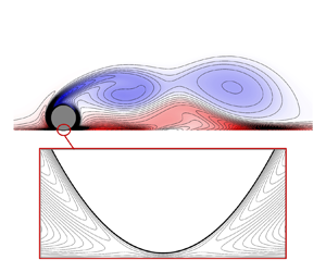
While the flow far from the interstice is independent of  $G/d$, the interstitial flow depends strongly on gap ratio. Figure 6 presents streamlines (contours of the streamfunction) in the interstice for $G/d = 10^{-3}$ and $10^{-4}$, and significant differences between the streamfunctions are observed between the two plots. In particular, the upstream and downstream saddle points (labelled $S_u$ and $S_d$ in figure 6) move closer to the contact point ( $x = 0$) as $G/d$ is decreased, and the total mass flow rate through the interstice also decreases with the gap ratio.

Figure 6. Contours of the streamfunction  $\varPsi$ near the interstice for the rolling cylinder at $Re = 100$, $k = 1$ and $t = 195$, for gap ratios (a) $G/d = 10^{-3}$ and (b) $G/d = 10^{-4}$, obtained using the single-domain, finite gap ratio method outlined in § 3.1. The contour increment is $\Delta \varPsi = 10^{-4}$, and axes are stretched vertically for clarity.
Figures 5 and 6 validate our assumption that the flow far from the interstice (the outer flow) is relatively independent of  $G/d$, while the interstitial (inner) flow depends strongly on the gap ratio. This can be demonstrated further by considering the pressure distribution on the surface of the cylinder. Since the wake is periodic, we compute the mean pressure $\bar {p}$, which is the pressure averaged over a single vortex-shedding cycle. We stress once again that since the single-domain method is used, a single pressure distribution, valid in both the inner and outer domains, is obtained for each gap ratio. This pressure distribution may be non-dimensionalised according to either outer variables (as $\bar {p}$) or inner variables (as $\hat {\bar {p}} = \bar {p}\,Re\,(G/d)^{3/2}/(2(1+k))$).
Figure 7(a) presents the mean pressure on the cylinder surface for  $Re = 100$, $k = 1$ and for a range of gap ratios, normalised by inner variables. The theoretical prediction from lubrication theory (2.22) is also shown. The profiles for $G/d = 10^{-3}$ and $10^{-4}$ are visually indistinguishable from the lubrication solution, confirming that the lubrication solution is valid in the inner region when $G/d \leq 10^{-3}$.

Figure 7. Mean pressure distribution on the cylinder surface normalised using (a) inner and (b,c) outer variables for  $Re = 100$ and $k=1$. Solid black lines indicate the analytical solutions for (a) lubrication theory (2.23) and (b) Stokes flow (2.10). A logarithmic $y$-axis is used in (c) to show that the outer solution approaches the Stokes flow solution in the region where the inner and outer solutions are asymptotically matched. The r.m.s. pressure is indicated by dashed lines in (a).
The lubrication solution for the inner region is obtained under the assumption of steady flow. To check this, we have also plotted profiles of the r.m.s. pressure, normalised by inner variables, in figure 7(a). The r.m.s. pressures are negligible when compared to the mean pressure profiles, therefore the assumption of steady flow is valid in the inner region.
Figure 7(b) shows the mean pressure on the cylinder surface normalised by outer variables, at  $Re = 100$, $k = 1$ and for a range of gap ratios. Far from the interstice (which is located at $\theta = 0,2{\rm \pi}$), the pressure distributions follow a single curve, confirming that the outer flow is independent of the gap ratio. The analytical solution for Stokes flow (2.10) is also presented in figure 7(b). While the inertial solutions for various $G/d$ follow a single curve, this curve differs substantially from the Stokes flow solution. Therefore, for inertial flows, there is a $G/d$-independent outer solution that differs from the Stokes flow solution.
Figure 7(c) shows the mean pressure on the cylinder surface in the region near the interstice, on a logarithmic  $y$-axis. For small $\theta$, the pressure profiles no longer follow a single $G/d$-independent solution, confirming that gap ratio effects are significant in the inner region. As $\theta$ is decreased, but still sufficiently large for gap ratio effects to be negligible, the inertial pressure distributions approach the Stokes flow solution. Therefore, the inertial outer-flow solution approaches the Stokes flow solution as $\theta$ approaches zero.
In this subsection, we have examined the flow over a rolling cylinder at a finite gap ratio, using a single-domain numerical computation. By interpreting this solution using the decomposition into inner and outer solutions, we have shown that for a sufficiently small gap ratio ( $G/d \leq 10^{-3}$):
(i) the inner flow is given by the analytic solution to lubrication theory;
(ii) the outer flow is independent of the gap ratio, but differs from the Stokes flow solution;
(iii) as the interstice is approached, the inertial outer-flow solution approaches the Stokes flow solution.
3.3. Obtaining the outer-flow solution for  $G/d = 0$

The results of § 3.2 show that the outer flow does not depend on  $G/d$, while the inner flow matches the analytic solution obtained using lubrication theory. Therefore, the single-domain approach is inefficient: numerical simulations are performed for each value of $G/d$, despite the fact that this affects only the inner flow, for which we already have an analytic solution. Therefore, we propose a new approach, where numerical simulations are performed only to obtain the $G/d$-independent outer solution. This solution can then be matched with the analytic solution to the inner flow to obtain a complete solution, valid for small gap ratios.
To obtain the  $G/d$-independent outer flow, we assume $G/d = 0$, thereby avoiding any finite-gap effects. Under this condition, the pressure approaches infinity at the contact point. The infinite pressures are avoided by removing the contact point from the computational domain, as shown in figure 8. New inlet/outlet boundaries are introduced at $\theta = \pm \theta _c$, and the velocity at these boundaries is set to the Stokes flow velocity profiles (2.7) and (2.8). Since the inertial outer flow solution is approximately equal to the Stokes flow solution for small $\theta$, this approximation is reasonable when $\theta _c$ is small. All other aspects of the numerical method, including the discretisation methods, boundary conditions and mesh scheme, are identical to the finite-gap simulations described in § 3.1.

Figure 8. For zero gap ratio simulations, the contact point is removed from the mesh and replaced with prescribed velocity boundaries, thereby avoiding the infinite pressure at the contact point. The parameters  $\Delta x$ and $N_y$ are the minimum cell spacing in the $x$-direction, and the number of cells across the film thickness, respectively.
Figure 9 presents vorticity contours obtained using the zero-gap method, for  $k = 1$, $Re = 100$ and $\theta _c = 0.01$. A transient animation is also provided in supplementary movie 1. The observed wake is nearly identical to that obtained using the single-domain simulations at $G/d = 10^{-3}$ and $10^{-4}$ (figures 5a,b), confirming that the proposed numerical approach is capable of predicting correctly the $G/d$-independent outer flow.

Figure 9. Vorticity contours for the rolling cylinder at  $Re = 100$, $k = 1$ and $t = 195$, obtained using the $G/d = 0$ method outlined in this subsection.
Figure 10(a) presents streamfunction contours near the contact point for  $G/d = 0$, $k = 1$ and $Re = 100$ obtained numerically with $\theta _c = 0.01$, while figure 10(b) presents streamfunction contours for Stokes flow (2.7) and (2.8). The predicted streamlines are nearly identical, confirming that the proposed method produces a velocity field that is approximately equal to the Stokes flow solution near the contact point. Moreover, the streamfunctions for the finite-gap cases, shown in figures 6(a,b), appear to converge towards the zero-gap solution as $G/d$ approaches zero.


Note that the outer solution obtained under the assumption  $G/d = 0$ is valid for $|\theta | \gg 2\sqrt {G/d}$ (see (2.27)), and the inner lubrication solution must be used when $|\theta |$ is below this value. To illustrate this point, figure 11(a) presents the mean pressure along the cylinder surface for $Re = 100$ and $k = 1$ obtained using the $G/d = 0$ approach outlined in this subsection, with $\theta _c = 0.01$, and a solution obtained using the conventional single-domain approach outlined in § 3.1, for finite gap ratio $G/d = 10^{-4}$. The Stokes flow solution for the outer flow (2.10) is also shown. All solutions are in good agreement between $\theta = 0.1$ and $\theta = 0.3$. However, finite-gap effects become significant for $\theta < 0.1$, and the $G/d = 0$ solution does not match the $G/d = 10^{-4}$ solution in this region.

Figure 11. (a) Mean pressure distribution on the cylinder surface for  $G/d = 0$ and $10^{-4}$ at $Re = 100$ and $k = 1$. (b) Difference between the mean pressure distributions for inertial flow and Stokes flow ( $\bar {p}-p_{Stokes}$) at $Re = 100$ and $k =1$.
Therefore, we introduce a transition angle  $\theta _0$ that separates the inner and outer solutions. By using the numerically obtained $G/d = 0$ outer solution for $|\theta | \geq \theta _0$, and the inner lubrication solution for $|\theta | < \theta _0$, we obtain a complete solution to the flow over a rolling cylinder at small, but finite, gap ratios. Importantly, $\theta _0$ must lie in the asymptotic matching region given by (2.27), therefore we require $2\sqrt {G/d} \leq \theta _0 \leq 2$. However, an additional constraint is that $\theta _0$ must be sufficiently small for inertial effects to be negligible. For this, we assume a film thickness Reynolds number $Re_h \lessapprox 1$, which by (2.14) requires $\theta _0 \lessapprox 2/\sqrt {Re}$. The range $0.1 \leq \theta \leq 0.3$ satisfies these conditions approximately for $G/d = 10^{-4}$ and $Re = 100$, therefore $\theta _0$ may take any value within this range. This is confirmed by the agreement between the inner and outer solutions over this range as observed in figure 11(a).
Figure 11(b) presents a comparison between the pressure distribution obtained under the zero-gap assumption, and the pressure obtained using the single-domain, finite-gap method. Here, we have subtracted the pressure from the Stokes flow solution (2.10) to show more clearly the inertial contribution. Away from the contact point, the single-domain and zero-gap solutions are nearly indistinguishable, therefore the zero-gap method proposed in this subsection is capable of determining the outer solution for finite-gap inertial flows, in the domain where this solution is applicable.
To summarise, we have shown that the inertial outer-flow solution obtained under the assumption  $G/d = 0$ correctly describes the flow in the outer region ( $|\theta | \gg 2/\sqrt {G/d}$) for small, but finite, gap ratios. We can then construct a complete solution by taking the numerically obtained outer solution for $|\theta | \geq \theta _0$, and using the inner lubrication solution for $|\theta | < \theta _0$, where $\theta _0$ is in the range $2\sqrt {G/d} \ll \theta _0 \ll 2$ and $\theta _0 \lessapprox 2/\sqrt {Re}$.
A grid resolution study is performed to confirm that a grid-independent outer-flow solutions is obtained. Table 3 lists four meshes used for this resolution study, including the number of cells in each mesh ( $N_c$), the representative cell sizes $\Delta x$ and $N_y$ (which are illustrated in figure 8), and the cut-out angle $\theta _c$. The time-mean and r.m.s. wake force and moment coefficients are also provided, and changes to these quantities between meshes 2 and 3 are below 1 %. Therefore, mesh 2 is considered sufficient to resolve the force and moment coefficients.
Table 3. Comparison in the predicted mean and r.m.s. wake force and moment coefficients for  $Re = 200$ and $k = 1$, evaluated using different grid resolutions. The relative differences between the predictions from meshes 2 and 3, and meshes 2 and 4, are given in parentheses.

Mesh 4 has the same resolution as mesh 2, but with  $\theta _c = 0.02$. Changes to the mean and r.m.s. wake force and moment coefficients between meshes 2 and 4 are below 0.02 %, confirming that $\theta _c = 0.01$ is sufficiently small to not introduce any significant errors.
Note that the minimum spacing in the  $x$-direction for mesh 2 is $\Delta x = 10^{-5}$, an order of magnitude smaller than the minimum spacing used for the finite $G/d$ computations (table 1). This was to reduce numerical errors associated with taking the difference of large numbers, which occurs in some of our analysis (see Appendix A). However, in Appendix A, we demonstrate that taking a larger value of $\Delta x = 5 \times 10^{-4}$ does not significantly affect the predicted force and moment coefficients.
In this subsection, we have simulated the flow over a cylinder at  $G/d = 0$ by removing the contact point from the computational domain in order to avoid the infinite pressure at the contact point. Pirozzoli, Orlandi & Bernardini (Reference Pirozzoli, Orlandi and Bernardini2012) have also performed numerical simulations of the rolling cylinder at $G/d = 0$, but do not report any difficulties with infinite pressures at the contact point. They report finite values for the drag coefficient at $G/d = 0$, in contrast with both the Stokes flow predictions and the present study. This discrepancy is likely a result of insufficient resolution to capture the flow near the contact point. They use a relatively low grid resolution of 40 points per cell radius, which means that near the contact point (specifically, for $-0.1 < x/d < 0.1$), the cylinder and the wall lie in the same computational cell. It is unlikely that the flow in this region is resolved satisfactorily, and the finite drag coefficients reported in that work are considered unreliable. However, since the outer flow is relatively insensitive to the flow near the contact point, the outer flow may be resolved correctly in their work.
3.4. Application of the proposed method to other problems
This paper has considered only the two-dimensional flow over a rolling cylinder. However, we anticipate that the approach outlined in this work may be extended to other rolling body problems, such as the flow over a rolling sphere or a finite cylinder (wheel). The method of matched asymptotic expansions has already been applied to the Stokes flow over a rolling sphere (Goldman et al. Reference Goldman, Cox and Brenner1967; O'Neill & Stewartson Reference O'Neill and Stewartson1967; Cooley & O'Neill Reference Cooley and O'Neill1968), to decompose the flow into inner and outer expansions. Therefore, we expect that the same method may be applied to the inertial flow over a rolling sphere.
We remark, however, that there are both qualitative and quantitative differences between the Stokes flows over rolling cylinders and spheres. For example, both the torque applied to a purely translating cylinder and the force applied to a purely rotating cylinder are zero (Jeffrey & Onishi Reference Jeffrey and Onishi1981), which is not the case for the rolling and translating spheres. Moreover, the force and moment applied to a rolling sphere both exhibit a logarithmic dependence on the gap ratio (Goldman et al. Reference Goldman, Cox and Brenner1967; O'Neill & Stewartson Reference O'Neill and Stewartson1967; Cooley & O'Neill Reference Cooley and O'Neill1968), compared to the  $(G/d)^{-1/2}$ dependence for the force and moment applied to the rolling cylinder (Merlen & Frankiewicz Reference Merlen and Frankiewicz2011). Despite these differences, the method of asymptotic expansions has been applied successfully to the Stokes flow over both cylinders and spheres, therefore the same approach should be applicable to the inertial flow over a rolling sphere.
The present paper has also neglected several physical effects that are likely to be present under typical experimental conditions, including surface roughness, cavitation and compressibility. These effects are likely to be significant in the inner region, therefore a modified lubrication theory must be used to account for these effects, such as Patir & Cheng (Reference Patir and Cheng1978) for rough surfaces, Almqvist et al. (Reference Almqvist, Fabricius, Larsson and Wall2014) for compressible and cavitating lubrication, or Harp & Salant (Reference Harp and Salant2001) for roughness-induced inter-asperity cavitation.
However, these effects are likely to be negligible in the outer region. Therefore, the present method will allow these effects to be considered separately from those of inertia, which affects only the outer solution. For example, the height of surface asperities is generally much smaller than the cylinder diameter, therefore surface roughness will be negligible in the outer region, except at high Reynolds numbers when the boundary layer thickness is comparable to the surface roughness height.
Similarly, the magnitude of the pressure in the outer region is generally small, except near the contact point where the outer solution is invalid. Hence we expect cavitation and compressibility effects to be confined to the inner region, at least for a wide range of experimental parameters. This is supported by the experimental observation that typically cavitation bubbles are confined to the inner region, for both spheres (Ashmore et al. Reference Ashmore, Del Pino and Mullin2005) and cylinders (Seddon & Mullin Reference Seddon and Mullin2006). Moreover, Ashmore et al. (Reference Ashmore, Del Pino and Mullin2005) are able to predict the motion of a sphere in a cavitating flow by assuming that flow outside the cavitation region is not affected by the formation of the cavitation bubble.
Seddon & Mullin (Reference Seddon and Mullin2006), however, have argued that, unlike the flow over a rolling sphere, cavitation in the interstice of the rolling cylinder modifies the outer flow to the extent that reverse rotation of the cylinder is observed. They argue that cavitation introduces a blockage effect, reducing the mass flow through the interstice. As a result, more fluid must flow around the upper surface of the cylinder, modifying the outer flow. However, the gap-to-diameter ratio also affects the volume flow rate of fluid through the interstice, yet the outer solution is insensitive to  $G/d$ (Merlen & Frankiewicz Reference Merlen and Frankiewicz2011). Therefore, there is no reason to assume that cavitation in the inner region directly affects the outer flow in this manner. A possible explanation for the observed reverse rotation of the cylinder is that cavitation modifies the inner-flow contribution to the moment applied to the cylinder, thereby altering the rotation rate. This would, of course, indirectly affect the outer flow, through its dependence on the parameter $k$. This proposal remains unconfirmed, however, and further research is needed to determine whether the effects of cavitation are confined to the inner region of the rolling cylinder flow.
4. Forces and moments
In this section, we discuss the computation of the force and moment coefficients using the inner and outer solutions. We first discuss the forces and moments for the Stokes flow solutions in § 4.1. Then the force and moment coefficients for inertial flows are discussed in §§ 4.2 and 4.3. Finally, in § 4.4, we present a parameter space study of the force and moment coefficients for a range of  $k$ and $Re$.
$Re$.
The total forces and moments applied to the cylinder are computed as
 $$\begin{gather} C_D = \int_0^{2{\rm \pi}} (-p \sin \theta + \tau_x )\,{\mathrm d} \theta, \end{gather}$$
 $$\begin{gather}C_L = \int_0^{2{\rm \pi}} (\,p \cos \theta + \tau_y )\,{\mathrm d} \theta, \end{gather}$$
 $$\begin{gather}C_M = \int_0^{2{\rm \pi}} (\tau_y \sin \theta + \tau_x \cos \theta ) \,{\rm d} \theta. \end{gather}$$
Each of these integrals is split into inner and outer regions as follows. First, the force and moment contributions from the outer region are written as
 $$\begin{gather} {C_D}_{,O}= \int_{\theta_0}^{2{\rm \pi} - \theta_0}( - p \sin \theta + \tau_x ) \,{\mathrm d} \theta, \end{gather}$$
 $$\begin{gather}{C_L}_{,O}= \int_{\theta_0}^{2{\rm \pi} - \theta_0}( p \cos \theta + \tau_y ) \,{\mathrm d} \theta, \end{gather}$$
 $$\begin{gather}{C_M}_{,O}= \int_{\theta_0}^{2{\rm \pi} - \theta_0}( \tau_y \sin \theta + \tau_x \cos \theta ) \,{\mathrm d} \theta, \end{gather}$$
while the force and moment contributions from the inner region are
 $$\begin{gather} {{C_D}}_{,I} = \int_{-\hat{x}_0}^{\hat{x}_0} [-4 (G/d) \hat{x} p + 2 (G/d)^{1/2} \tau_x] \,{\mathrm d} \hat{x}, \end{gather}$$
 $$\begin{gather}{{C_L}}_{,I} = \int_{-\hat{x}_0}^{\hat{x}_0} 2(G/d)^{1/2} ( p + \tau_y ) \,{\mathrm d} \hat{x}, \end{gather}$$
 $$\begin{gather}{{C_M}}_{,I}= \int_{-\hat{x}_0}^{\hat{x}_0}[ 2(G/d)^{1/2}\tau_x + 4(G/d)\hat{x}\tau_y ]\,{\mathrm d} \hat{x}, \end{gather}$$
where  $\hat {x}_0 \approx \sin \theta _0 / (2 \sqrt {G/d})$, and subscripts $I$ and $O$ denote the inner and outer regions, respectively. As discussed in § 3.3, the parameter $\theta _0$ denotes the boundary between the inner and outer regions, and must lie in the region where the inner and outer solutions are asymptotically matched ( $2\sqrt {G/d} \ll \theta _0 \ll 2$ and $\theta _0 \lessapprox 2/\sqrt {Re}$). Within this range, the individual force and moment contributions from the inner and outer regions may depend on the value of $\theta _0$, but the total forces and moments must be independent of $\theta _0$.
4.1. Stokes flow
Substituting (2.23) and (2.25) into (4.7)–(4.9), we obtain the following expressions for the contributions to the force and moment coefficients from the inner region:
 $$\begin{gather} {C_D}_{,I} = \frac{8}{Re\,(G/d)^{1/2}} \tan^{-1} \hat{x}_0, \end{gather}$$
 $$\begin{gather}{C_L}_{,I} = 0, \end{gather}$$
 $$\begin{gather}{{C_M}}_{,I} = \frac{8}{Re\,(G/d)^{1/2}} \left[-k \tan^{-1} \hat{x}_0 + (1+k)\, \frac{\hat{x}_0}{1+\hat{x}_0^2}\right]. \end{gather}$$
Similarly, substituting (2.10)–(2.12) into (4.4)–(4.6) gives expressions for the contribution to the force and moment coefficients from the outer region for Stokes flow:
 $$\begin{gather} {{C_D}}_{,O,S}= \frac{8}{Re}\,[ \cot(\theta_0/2) + k \sin \theta_0 ], \end{gather}$$
 $$\begin{gather}{{C_L}}_{,O,S} = 0, \end{gather}$$
 $$\begin{gather}{{C_M}}_{,O,S} =-\frac{8(2k+1)}{Re}\cot(\theta_0/2), \end{gather}$$
where a subscript  $S$ is used for the Stokes flow solutions. When $\theta _0$ is within the asymptotic matching region ( $\hat {x}_0\gg 1$ and $\theta _0\ll 1$), these are approximated as
 $$\begin{gather} {{C_D}}_{,I} \approx \frac{8}{Re\,(G/d)^{1/2}}\left[ \frac{\rm \pi}{2} - \frac{1}{\hat{x}_0}\right], \end{gather}$$
 $$\begin{gather}{{C_M}}_{,I}\approx \frac{8}{Re\,(G/d)^{1/2}}\left[ - \frac{\rm \pi}{2}\,k + (2k+1)\,\frac{1}{\hat{x}_0}\right], \end{gather}$$
 $$\begin{gather}{{C_D}}_{,O,S} \approx \frac{8}{Re\,(G/d)^{1/2}}\, \frac{1}{\hat{x}_0}, \end{gather}$$
 $$\begin{gather}{{C_M}}_{,O,S} \approx-\frac{8(2k+1)}{Re\,(G/d)^{1/2}}\,\frac{1}{\hat{x}_0}, \end{gather}$$
and the total force and moment coefficients for Stokes flow are therefore given by
 $$\begin{gather} {C_D}_{,S} = \frac{4{\rm \pi}}{Re\,(G/d)^{1/2}}, \end{gather}$$
 $$\begin{gather}{C_L}_{,S} = 0, \end{gather}$$
 $$\begin{gather}{C_M}_{,S} =-\frac{4{\rm \pi} k}{Re\,(G/d)^{1/2}}, \end{gather}$$
in agreement with Merlen & Frankiewicz (Reference Merlen and Frankiewicz2011). Importantly, while the drag and moment coefficients from both the inner and outer regions ((4.16)–(4.19)) depend on the boundary between the inner and outer regions ( $\theta _0$), the total force and moment coefficients ((4.20)–(4.22)) do not.
4.2. Inertial flow
We now consider the force and moment coefficients for inertial flow. Since inertial effects are negligible in the inner region, the force and moment coefficients for the inner region ( ${{C_D}}_{,I}$, ${{C_L}}_{,I}$ and ${{C_M}}_{,I}$) are given by the lubrication solution (4.10)–(4.12). The force and moment coefficients for the outer region ( ${{C_D}}_{,O}$, ${{C_L}}_{,O}$ and ${{C_M}}_{,O}$) are evaluated using (4.4)–(4.6), with the pressure and velocity fields obtained numerically using the $G/d = 0$ approach described in § 3.3. In this subsection, we consider the mean force and moment coefficients averaged over one period of the saturated vortex shedding state, which are denoted $\overline {{C_D}}_{,O}$, $\overline {{C_L}}_{,O}$ and $\overline {{C_M}}_{,O}$, respectively. The transient behaviour of the force and moment coefficients is considered later, in § 4.3. Only the inertial outer-flow solutions are time-averaged, as both the inner lubrication and outer Stokes flow solutions are steady in time. Note that equations derived in this subsection are expressed in terms of instantaneous quantities, for generality. The corresponding expressions for time-averaged quantities are identical.
Figure 12(a) plots the numerically obtained values of  $\overline {{C_D}}_{,O}$, $\overline {{C_L}}_{,O}$ and $\overline {{C_M}}_{,O}$ against $\theta _0$, for $Re = 100$ and $k = 1$. The corresponding force and moment coefficients for Stokes flow ((4.13)–(4.15)) are indicated by dashed lines. The force and moment coefficients for inertial flow are all greater in magnitude than the corresponding values for Stokes flow, indicating that inertial effects increase the drag, lift and torque applied to the cylinder. Due to the pressure singularity at the contact point, the drag and moment coefficients are singular at $\theta _0 = 0$. However, the lift coefficient remains finite as $\theta _0$ approaches $0$.
$0$.

Figure 12. (a) Variation in the force and moment coefficients for the outer region ( $\overline {{C_D}}_{,O}$, $\overline {{C_L}}_{,O}$ and $\overline {{C_M}}_{,O}$) against $\theta _0$ for $Re = 100$ and $k = 1$ (solid lines) as well as the Stokes flow predictions (4.13)–(4.15), shown with dashed lines. (b) Variation of the inertial contributions to the outer-flow force and moment coefficients ( $\Delta \overline {{C_D}}_{,O}$, $\Delta \overline {{C_L}}_{,O}$ and $\Delta \overline {{C_M}}_{,O}$) with $\theta _0$ for $Re = 100$ and $k = 1$. Dashed lines indicate the limiting behaviour for small $\theta _0$.
The force and moment coefficients for a finite gap ratio are given as the sums of contributions from the inner and outer solutions:
 \begin{equation} C_D = {{C_D}}_{,I} + {{C_D}}_{,O},\quad C_L = {{C_L}}_{,I} + {{C_L}}_{,O},\quad C_M = {{C_M}}_{,I} + {{C_M}}_{,O}. \end{equation}
 This is illustrated in figure 13, which plots the balance between the inner and outer drag coefficients against  $\theta _0$, for $G/d = 10^{-4}$, $Re = 100$ and $k = 1$. Here, ${{C_D}}_{,I}$ is given by (4.10), while $\overline {{C_D}}_{,O}$ is evaluated numerically using the $G/d = 0$ method described in § 3.3. While both ${{C_D}}_{,I}$ and $\overline {{C_D}}_{,O}$ vary with $\theta _0$, the total drag coefficient (4.23a–c) is approximately constant when $\theta _0$ is within the asymptotic matching region (estimated to be $0.1\leq \theta _0 \leq 0.3$ at $G/d = 10^{-4}$ and $Re = 100$; see § 3.3). Therefore, we can take any $\theta _0$ within this range, and obtain the force and moment coefficients through (4.23a–c). The dashed line in figure 13 indicates the drag coefficient obtained using the single-domain computation at $G/d = 10^{-4}$, and the drag coefficient predicted by (4.23a–c) is in excellent agreement with this value when $\theta _0$ is in the asymptotic matching region.

Figure 13. Contributions to the drag coefficient from the inner and outer regions, for  $G/d = 10^{-4}$, $Re = 100$ and $k = 1$.
While (4.23a–c) is sufficient to obtain the force and moment coefficients for a given  $G/d$, a more convenient approach is to first define the ‘wake’ force/moment coefficients as
 \begin{equation} {C_D}_{,{wake}} = C_D - {{C_D}}_{,S},\quad {C_L}_{,{wake}} = C_L - {{C_L}}_{,S},\quad {C_M}_{,{wake}} = C_M - {{C_M}}_{,S}, \end{equation}
which we interpret as representing the inertial contribution to the total force and moment coefficients. Importantly, we will show that the wake force and moment coefficients are approximately independent of  $G/d$, and can be estimated using the outer-flow solution alone. Thus this decomposition is more convenient than (4.23a–c), as the $G/d$ dependence is contained entirely within the Stokes flow terms, for which we have a known analytic solution (4.20)–(4.22).
Using (4.23a–c) and (4.24a–c), the wake force and moment coefficients can be expressed as
 \begin{equation} {C_D}_{,{wake}} = \Delta {{C_D}}_{,O}(\theta_0),\quad {C_L}_{,{wake}} = \Delta {{C_L}}_{,O}(\theta_0),\quad {C_M}_{,{wake}} = \Delta {{C_M}}_{,O}(\theta_0), \end{equation}
where
 \begin{align} \Delta {{C_D}}_{,O} = {{C_D}}_{,O} - {{C_D}}_{,O,S},\quad \Delta {{C_L}}_{,O} = {{C_L}}_{,O} - {{C_L}}_{,O,S},\quad \Delta {{C_M}}_{,O} = {{C_M}}_{,O} - {{C_M}}_{,O,S} \end{align}
are the inertial contributions to the force and moment coefficients from the outer flow, which are plotted in figure 12(b). While the total force and moment coefficients are singular at  $\theta _0 = 0$, the inertial contributions remain bounded.
Since the conditions for asymptotic matching require  $\theta _0 \ll 1$, we consider the behaviour of $\Delta \overline {{C_D}}_{,O}$, $\Delta \overline {{C_M}}_{,O}$ and $\Delta \overline {{C_L}}_{,O}$ for small $\theta _0$. The asymptotic behaviours of these quantities for small $\theta _0$ are represented by dashed lines in figure 12(b). These are obtained by fitting fourth-order polynomials to each of these quantities in the range $0.1 \leq \theta _0 \leq 0.5$, and retaining terms up to first order in $\theta _0$. (The range $\theta _c \leq \theta _0 \leq 0.1$ is omitted from the polynomial fit, due to numerical issues associated with large pressure magnitudes near the contact point, as discussed in Appendix A.) The drag and moment coefficients are approximately constant, therefore the first-order terms are also neglected, i.e.
 \begin{equation} \Delta {{C_D}}_{,O} \approx \Delta {{C_D}}_{,O}|_{\theta_0=0} + \textit{O}(\theta_0^2),\quad \Delta {{C_M}}_{,O} \approx \Delta {{C_M}}_{,O}|_{\theta_0=0} + \textit{O}(\theta_0^2), \end{equation}
while the lift coefficient is approximately linear, i.e.
 \begin{equation} \Delta {{C_L}}_{,O} \approx \Delta {{C_L}}_{,O}|_{\theta_0=0} + \textit{O}(\theta_0).\end{equation}
Terms such as  $\Delta {{C_D}}_{,O}|_{\theta _0=0}$ are obtained as the constant terms in the polynomial fits, which, for the $Re = 100$ and $k = 1$ case shown in figure 12(b), are $\Delta {{C_D}}_{,O}|_{\theta _0=0} = 1.8973$, $\Delta {{C_L}}_{,O}|_{\theta _0=0} = 1.9821$ and $\Delta {{C_M}}_{,O}|_{\theta _0=0} = -0.3099$.
Based on the conditions required for asymptotic matching between the inner and outer solutions, we assume that  $\theta _0 \propto \sqrt {G/d}$. Then, by using (4.27a,b) and (4.28), we can estimate the wake force and moment coefficients from the outer flow solution alone:
 $$\begin{gather} {C_D}_{,wake} = \Delta {{C_D}}_{,O}|_{\theta_0 = 0} + \textit{O}(G/d), \end{gather}$$
 $$\begin{gather}{C_L}_{,wake} = \Delta {{C_L}}_{,O}|_{\theta_0 = 0} + \textit{O}(\sqrt{G/d}), \end{gather}$$
 $$\begin{gather}{C_M}_{,wake} = \Delta {{C_M}}_{,O}|_{\theta_0 = 0} + \textit{O}(G/d). \end{gather}$$
Note that the predicted wake drag and moment coefficients are of a higher order of accuracy than the wake lift coefficient.
Equations (4.29)–(4.31) allow the wake force and moment coefficients to be estimated from the outer solution alone. The total force and moment coefficients are then obtained by adding the Stokes flow force and moment coefficients:
 \begin{equation} C_D = {{C_D}}_{,S} + {C_D}_{,{wake}},\quad C_L = {C_L}_{,{wake}},\quad C_M = {{C_M}}_{,S} + {C_M}_{,{wake}}. \end{equation}
Moreover, the wake force and moment coefficients are approximately independent of  $G/d$, for small gaps. The gap ratio affects the force and moment coefficients through only the Stokes flow terms, for which analytical expressions are given in (4.20)–(4.22).
We now validate the proposed approach for determining the force and moment coefficients. Figure 14 presents the variation in the force and moment coefficients against  $G/d$ for $Re = 100$ and $k = 1$, determined using finite gap ratio numerical simulations (open circles) and the Stokes flow predictions (solid lines), and by using the wake force/moment predictions from the zero-gap solution ((4.32a–c), dashed lines). For both ${C_D}$ and ${C_M}$ (figures 14a,b), the predictions from the finite gap ratio simulations differ from the Stokes flow predictions by a constant amount, which is equal to the wake drag/moment coefficients predicted from the zero-gap outer flow ((4.29) and (4.31)). Therefore, (4.32a–c) is found to predict accurately the drag and moment coefficients, for a wide range of gap ratios.

Figure 14. Comparison between the predicted force and moment coefficients (a)  $C_D$, (b) $C_M$ and (c) $C_L$ against gap ratio using single-domain, finite $G/d$ numerical simulations (circles) and the Stokes flow solution (solid lines), and by using the wake force and moment coefficients obtained from the $G/d = 0$ solution ((4.32a–c), dashed lines), for $Re = 100$ and $k = 1$.
Figure 14(c) presents the  $\overline {C_L}$ predicted from finite $G/d$ simulations, as well as predicted using (4.32a–c). While (4.32a–c) predicts a constant lift coefficient, the numerically computed values decrease with increasing $G/d$. The numerically obtained $\overline {C_L}$ vary approximately linearly with $\sqrt {G/d}$, which is consistent with the order of the error estimate given in (4.30). The value of ${C_L}_{,{wake}}$ predicted from the outer-flow solution (4.30) is the upper limit on the lift coefficient, as $G/d$ approaches 0. This is confirmed by extrapolating $\overline {C_L}$ from the finite $G/d$ simulations to $G/d = 0$, which gives a prediction $\overline {C_L} = 1.9921$, and this is within $0.5\,\%$ of the prediction obtained using (4.30).
We remark that finite-gap simulations could not be performed for  $G/d < 10^{-4}$, due to numerical difficulties associated with small cell sizes. However, the force and moment predictions obtained using (4.29)–(4.31) and (4.32a–c) are valid for arbitrarily small $G/d$, and the accuracy of these predictions increases as $G/d$ approaches zero. Therefore, in addition to reducing the parameter space to only two variables, the proposed method allows the force and moment predictions to be obtained for arbitrarily small $G/d$, while avoiding the numerical difficulties that occur in finite-gap simulations.
4.3. Force and moment coefficients for unsteady flow
While only time-averaged force and moment coefficients were discussed in § 4.2, (4.29)–(4.32a–c) are also valid for the instantaneous force and moment coefficients in an unsteady flow. Figure 15 presents the time history of  ${{C_D}}_{,{wake}}$, ${{C_L}}_{,{wake}}$ and ${{C_M}}_{,{wake}}$ for $Re = 100$ and $k = 1$ obtained from the $G/d = 0$ numerical simulations using (4.29)–(4.31). The wake force and moment coefficients predicted using finite $G/d$ simulations are also plotted in figure 15. To aid comparison, the flow times have been shifted so that $t = 0$ corresponds to the maximum drag coefficient. Since the wake is in the saturated state of periodic vortex shedding, the predicted wake force and moment coefficients are periodic, and two complete wake cycles are shown.

Figure 15. Time history of (a)  ${C_D}_{,{wake}}$, (b) ${C_M}_{,{wake}}$ and (c) ${C_L}_{,{wake}}$ for a range of gap ratios. Flow times are shifted so that $t = 0$ corresponds to the maximum value of ${C_D}_{,{wake}}$.
Figures 15(a,b) show that the instantaneous values of  ${C_D}_{,{wake}}$ and ${C_M}_{,{wake}}$ are approximately independent of gap ratio, with some mild discrepancy observed between different values of $G/d$. On the other hand, figure 15(c) shows that the instantaneous value of ${C_L}_{,{wake}}$ generally increases as $G/d$ decreases, consistent with results presented in § 4.2. However, while the mean value of ${C_L}_{,{wake}}$ increases with $G/d$, the amplitude of the oscillations in ${C_L}_{,{wake}}$ appears to be relatively independent of $G/d$.
These qualitative observations are confirmed by table 4, which presents the mean and r.m.s. values of the wake force and moment coefficients, as well as the Strouhal number, for each  $G/d$. For all quantities apart from the mean lift coefficient $\overline {{C_L}}_{,{wake}}$, the relative error between the predictions for $G/d = 10^{-3}$ and $G/d = 0$ are below $1.5\,\%$, while the relative errors between the $G/d = 10^{-4}$ and $G/d = 0$ predictions for all quantities are below $0.7\,\%$. We remark that the discretisation errors from the grid resolution study are also of order $1\,\%$, so it is unclear how much of the observed discrepancy is due to finite-gap effects and how much is due to grid resolution errors.
Table 4. Dependence of the mean and r.m.s. wake force and moment coefficients, as well as the Strouhal number ( $St$), with gap ratio, at $Re = 100$ and $k = 1$. The relative differences between the finite-gap and zero-gap values are given in parentheses.

Differences in  $\overline {C_L}_{,{wake}}$ between the finite-gap and zero-gap solutions are substantial for both $G/d = 10^{-3}$ and $G/d = 10^{-2}$, but below $0.7\,\%$ for $G/d = 10^{-4}$. As discussed in § 4.2, the value of $\overline {C_L}_{,{wake}}$ predicted from the $G/d = 0$ simulations using (4.30) is an upper bound on the true value of $\overline {C_L}_{,{wake}}$, with an error approximately proportional to $\sqrt {G/d}$. While the mean lift coefficient shows strong dependence on $G/d$, ${C_L}_{,{rms}}$ shows only weak dependence on $G/d$, and the differences in ${C_L}_{,{rms}}$ between the finite-gap and zero-gap solutions are comparable to the corresponding differences in both ${C_M}_{,{rms}}$ and ${C_D}_{,{rms}}$. Therefore, while the mean value of ${C_L}_{,{wake}}$ depends on $G/d$, the amplitude of oscillations of ${C_L}_{,{wake}}$ is relatively insensitive to $G/d$.
Differences in  ${C_D}_{,{rms}}$, ${C_L}_{,{rms}}$ and ${C_M}_{,{rms}}$ between the $G/d = 10^{-2}$ and $G/d = 0$ predictions are substantial. This is not surprising, given that the decomposition into inner and outer solutions is valid only for small $G/d$. Moreover, figure 7(a) demonstrates that the lubrication solution to the inner region is not valid for $G/d = 10^{-2}$. Despite these observations, the values of $\overline {C_D}_{,{wake}}$ and $\overline {C_M}_{,{wake}}$ predicted for $G/d = 10^{-2}$ are within $0.5\,\%$ of those predicted using $G/d = 0$, therefore the decomposition into inner and outer flows is surprisingly effective in predicting the mean drag and moment coefficients, even for relatively large $G/d$ where the decomposition into inner and outer flows is not strictly valid.
4.4. Parameter space
One of the main advantages of the decomposition into inner and outer flows presented in this paper is that the wake force and moment coefficients predicted from the outer flow depend on only two variables,  $Re$ and $k$, substantially reducing the parameter space to be explored by numerical simulations. In this subsection, we present numerical computations of the mean and r.m.s. wake force and moment coefficients as functions of $Re$ and $k$. We remark that the predicted values of $\overline {{C_L}}_{,{wake}}$ presented in this subsection represent the upper bounds on the lift coefficient, and have an error of order $\sqrt {G/d}$.
We first consider the effect of  $Re$ on the wake force and moment coefficients for $k = 1$. Figure 16(a) presents the variation of $\overline {C_D}_{,{wake}}$, $\overline {C_L}_{,{wake}}$ and $\overline {C_M}_{,{wake}}$ against $Re$, for $k = 1$ and for both unsteady (circles) and steady (triangles) two-dimensional flow. For steady flow, the magnitudes of the mean wake drag, lift and moment coefficients all decrease monotonically with increasing $Re$. For $k = 1$, the two-dimensional wake becomes unsteady for $Re > 88$ (Houdroge et al. Reference Houdroge, Leweke, Hourigan and Thompson2017). However, there is little difference in the values of $\overline {C_L}_{,{wake}}$ and $\overline {C_M}_{,{wake}}$ between the steady and unsteady flows above this critical Reynolds number. The transition to unsteady flow is associated with a significant increase in the mean wake drag coefficient ( $\overline {C_D}_{,{wake}}$), compared to the steady flow. This is in agreement with Houdroge et al. (Reference Houdroge, Leweke, Hourigan and Thompson2017), who find that two-dimensional vortex shedding results in an increase in drag coefficient compared to steady flow, with only small changes to the lift coefficient.

Figure 16. Variation of (a) mean and (b) r.m.s. wake force and moment coefficients against  $Re$ for $k = 1$. Circles and triangles indicate the predictions for unsteady and steady flow, respectively.
Figure 16(b) presents the variation of the r.m.s. force and moment coefficients  ${C_D}_{,{rms}}$, ${C_L}_{,{rms}}$ and ${C_M}_{,{rms}}$ against $Re$ for $k = 1$. Below the critical Reynolds number $Re_{c,2D} = 88$, the r.m.s. force and moment coefficients are zero, indicating steady flow. As $Re$ is increased beyond this critical value, the r.m.s. force and moment coefficients increase monotonically.
Figure 17 presents a comparison between the predicted mean drag and lift coefficients at  $G/d = 0.005$ and $k = 1$ using the wake drag approach (4.32a–c) and with numerical results given by Houdroge et al. (Reference Houdroge, Leweke, Hourigan and Thompson2017). Good agreement is observed between the predicted mean drag coefficients, while our method slightly overestimates the lift coefficient, which is expected given that the error in the lift coefficient is of order $\sqrt {G/d}$.

Figure 17. Comparison between the predicted mean drag and lift coefficients for unsteady flow at  $k = 1$ and $G/d = 0.005$ using the present method ( $\circ$) and Houdroge et al. (Reference Houdroge, Leweke, Hourigan and Thompson2017) ( $\times$).
We now consider the effect of varying rotation rate ( $k$) for a fixed Reynolds number $Re = 100$. Figure 18(a) presents the variation of $\overline {C_D}_{,{wake}}$, $\overline {C_L}_{,{wake}}$ and $\overline {C_M}_{,{wake}}$ against $Re$ for $k = 1$ for both unsteady (circles) and steady (triangles) two-dimensional flow. The magnitudes of both $\overline {C_D}_{,{wake}}$ and $\overline {C_M}_{,{wake}}$ increase monotonically with $k$, while $\overline {C_L}_{,{wake}}$ takes a minimum value between $k = 0.5$ and $k = 0.75$.

Figure 18. Variation of (a) mean and (b) r.m.s. wake force and moment coefficients against  $k$ for $Re = 100$. Circles and triangles indicate the predictions for unsteady and steady flow, respectively.
Figure 18(b) presents the variation of the r.m.s. force and moment coefficients against  $k$ for $Re = 100$. At this Reynolds number, the transition between steady and unsteady flow occurs between $k = 0.25$ and $k = 0.5$, and the r.m.s. force and moment coefficients increase monotonically with $k$ beyond the transition to unsteady flow. This suggests that the critical Reynolds number for transition to unsteady flow decreases with increasing $k$, in agreement with Stewart et al. (Reference Stewart, Thompson, Leweke and Hourigan2010b). Figure 18(a) shows little difference in the predicted mean lift and moment coefficients between steady and unsteady flow; however, the transition to unsteady flow is associated with an increase in the mean drag coefficient.
Finally, we consider the effects of varying both  $Re$ and $k$ for two-dimensional, unsteady flow. Figure 19 presents contours of $\overline {C_D}_{,{wake}}$, $\overline {C_L}_{,{wake}}$, $\overline {C_M}_{,{wake}}$, ${C_D}_{,{rms}}$, ${C_L}_{,{rms}}$ and ${C_M}_{,{rms}}$ against both $Re$ and $k$, for two-dimensional unsteady flow. The solid black line marks the approximate transition from steady to unsteady flow, which is estimated using the r.m.s. lift coefficient. The critical Reynolds number $Re_{c,2D}$ decreases with increasing rotation rate, in agreement with Stewart et al. (Reference Stewart, Thompson, Leweke and Hourigan2010b). Within the unsteady regime, the r.m.s. force and moment coefficients (figures 19d–f) increase with both $k$ and $Re$.
$Re$.

Figure 19. Contours of the mean and r.m.s. wake force/moment coefficients (a)  $\overline {C_D}_{,{wake}}$, (b) $\overline {C_L}_{,{wake}}$, (c) $\overline {C_M}_{,{wake}}$, (d) ${C_D}_{,{rms}}$, (e) ${C_L}_{,{rms}}$ and (f) ${C_M}_{,{rms}}$, against $k$ and $Re$. The thick black line delineates between steady and unsteady two-dimensional flows.
Within the steady regime,  $\overline {C_D}_{,{wake}}$ increases with increasing $k$, but decreases with increasing $Re$ (figure 19a). In the unsteady regime, however, $\overline {C_D}_{,{wake}}$ increases with both increasing $k$ and increasing $Re$. The wake moment coefficient $\overline {C_M}_{,{wake}}$ depends predominantly on $Re$ within the steady regime, but is relatively insensitive to $Re$ in the unsteady regime (figure 19c). In particular, $\overline {C_M}_{,{wake}}$ decreases with increasing $Re$ in the steady regime, and increases with increasing $k$ in the unsteady regime. Finally, $\overline {C_L}_{,{wake}}$ decreases with increasing $Re$ in both the steady and unsteady regimes (figure 19b). For a fixed Reynolds number, $\overline {C_L}_{,{wake}}$ takes a minimum value for an intermediate value of $k$ between approximately $k = 0.5$ and $k = 0.75$; however, there is insufficient resolution in the $k$-direction to determine accurately the precise value of $k$ that minimises $\overline {C_L}_{,{wake}}$.
5. Conclusions
We have analysed and interpreted the two-dimensional flow over a circular cylinder translating along a plane wall, and with varying degrees of slip, including no-slip, using the method of matched asymptotic expansions. We consider an inner lubrication flow, which is valid near the thin interstice between the cylinder and the wall, and an inertial outer flow, which is valid far from the interstice. While three dimensionless parameters –  $Re$,
$Re$,  $k$ and $G/d$ – are needed to characterise this flow, the outer flow is independent of $G/d$, and depends only on $Re$ and $k$.
$k$.
Numerical simulations of the outer flow were performed over a range of  $Re$ and $k$. To avoid the numerical difficulties associated with infinite pressures arising at the contact point, the contact point itself was removed from the computational domain. The velocity corresponding to the Stokes flow solution was used as a prescribed-velocity boundary condition near the contact point. To complete this model, the pressure and velocity distributions in the inner flow were then obtained as an analytic solution to the Reynolds equation.
The effects of inertia on the force and moment coefficients are characterised by the wake force and moment coefficients, which can be estimated directly from the outer solution as functions of  $Re$ and $k$. The total force and moment coefficients can then be determined by adding to these the corresponding force and moment coefficients for Stokes flow. We find that the wake drag and moment coefficients are relatively independent of $G/d$, and therefore can be determined to a high accuracy using the outer solution alone. The wake lift coefficient, however, decreases linearly with $\sqrt {G/d}$, and the outer solution provides only the maximum limiting value of the wake coefficient.
One of the main benefits of the decomposition into inner and outer flows is a reduction in the parameter space to be explored by numerical simulations. In particular, the gap ratio effects are completely contained in the analytic Stokes flow terms, and numerical simulations for the outer flow depend only on  $Re$ and $k$. To obtain a complete dynamical model for the motion of a rolling body, we require the force and moment coefficients as functions of $k$,
$k$,  $Re$ and $G/d$. The present method substantially reduces the computational effort required to construct such a model.
Additionally, numerical simulations become increasingly impractical as  $G/d$ is decreased, due to the small cell sizes required to resolve the interstitial flow, as well as the large pressure magnitudes that occur in the interstice. Since the inner lubrication flow is obtained analytically, rather than numerically, these issues are avoided when using the method proposed in this paper.
Moreover, many physical effects, including cavitation, compressibility and surface roughness, are likely to be significant only in the inner region. The present work separates these effects conceptually from those of inertia, which affects only the outer region. Therefore, the method presented in this work can be extended readily to rough cylinders, as well as cavitating and compressible flows, by using a modified Reynolds equation that accounts for these effects in the inner region.
Finally, we remark that the method presented in this work can be extended to flows over other rolling bodies. For example, the forces and moments applied to a rolling sphere in a Stokes flow are also obtained by a decomposition into inner and outer flows (Goldman et al. Reference Goldman, Cox and Brenner1967; O'Neill & Stewartson Reference O'Neill and Stewartson1967), and we anticipate that the present approach can be used to obtain the wake force and moment coefficients for a rolling sphere in an inertial flow as functions of only  $Re$ and $k$. This approach may also be useful for understanding a range of other rolling bodies, including finite cylinders (wheels), or asymmetrically shaped particles. These possibilities will be explored in future research.
Supplementary movies
A supplementary movie is available at https://doi.org/10.1017/jfm.2023.296.
Funding
This work was supported by the Australian Government through the Australian Research Council's Discovery Projects funding scheme (projects DP200100704 and DP210100990), and by computational resources provided by the Australian Government through the National Computational Infrastructure (NCI) and Pawsey Supercomputer Centre (merit grant d71) under the National Computational Merit Allocation Scheme.
Declaration of interests
The authors report no conflict of interest.
Appendix A. Computing the inertial part of the outer flow solution
Computing the wake force and moment coefficients requires subtracting the Stokes flow solutions from the numerically obtained outer-flow solution. Since the pressure and wall shear stresses for the outer flow approach infinity as  $\theta \rightarrow 0$, this requires taking the difference of two large, and nearly equal, numbers, when $\theta$ is small. This amplifies numerical errors near the contact point, making the wake force and moment computations unreliable when $\theta _0$ is small.
To illustrate this point, figure 20(a) plots the mean pressure obtained numerically using the zero-gap approach outlined in § 3.3, for  $k = 1$ and $Re = 100$. Four different meshes are used, with values of $\Delta x$ between $10^{-5}$ and $5\times 10^{-4}$, and all other parameters are similar to mesh 2 from table 3. The pressure distribution for Stokes flow (2.10) is also shown. The pressures obtained on each mesh are nearly identical to the Stokes flow pressure when $\theta$ is small, and both profiles approach infinity as $\theta$ approaches zero. Therefore, computing the pressure difference ( $\bar {p} - p_{Stokes}$) near $\theta = 0$ requires taking the difference of two large, but nearly equal, numbers.

Figure 20. (a) Profiles of the mean pressure  $\bar {p}$ near the contact point, and (b) the difference between the mean pressure for inertial and Stokes flow solutions ( $\bar {p}-p_{Stokes}$), at $Re = 100$ and $k = 1$. Four different meshes are used, with $\Delta x$ between $10^{-5}$ and $5\times 10^{-4}$.
Figure 20(b) plots profiles of the pressure difference ( $\bar {p} - p_{Stokes}$) against $\theta$. While the total pressure $\bar {p}$ is grid-independent (figure 20a), the computed pressure difference shows a clear grid dependency, as well as large oscillations, when $\theta$ is small, presumably due to numerical errors arising from subtracting large numbers. The numerical oscillations are reduced as $\Delta x$ is decreased, and there appears to be a clear trend in convergence towards a grid-independent solution as $\Delta x$ is decreased. Therefore, a fine mesh with $\Delta x = 10^{-5}$ was used in the present study.
We now consider the force and moment coefficients. Figure 21 plots profiles of  $\Delta \overline {{C_D}}_{,O}$ (defined in (4.26a–c)) against $\theta _0$, computed on each of the four numerical grids. Numerical errors associated with taking the difference of large numbers are significant when $\theta _0 < 0.1$. These errors are most noticeable when $\Delta x = 5 \times 10^{-4}$, but visible numerical artefacts are still observed for the finer grids. We find similar errors for the other force and moment coefficients $\Delta \overline {{C_L}}_{,O}$ and $\Delta \overline {{C_M}}_{,O}$ (not shown for brevity).

Figure 21. Profiles of the inertial part of the outer-flow contribution to the drag coefficient ( $\Delta {{C_D}}_{,O}$) against $\theta _0$, at $Re = 100$ and $k=1$, computed using four different meshes with $\Delta x$ between $10^{-5}$ and $5\times 10^{-4}$. The dashed line indicates the polynomial fit obtained for the $\Delta x = 10^{-5}$ solution.
Therefore, we consider the computed profiles of  $\Delta \overline {{C_D}}_{,O}$, $\Delta \overline {{C_L}}_{,O}$ and $\Delta \overline {{C_M}}_{,O}$ to be unreliable when $\theta _0 < 0.1$. To estimate the wake force and moment coefficients, we propose fitting a fourth-order polynomial to these terms over the interval $0.1 < \theta _0 < 0.5$, and using this polynomial fit to estimate the wake force and moment coefficients, as described in § 4.2. The polynomial fit for $\Delta \overline {{C_D}}_{,O}$ obtained using the $\Delta x = 10^{-5}$ solution is indicated by a dashed line in figure 21, and appears to be a good approximation for the ‘expected’ behaviour of $\Delta \overline {{C_D}}_{,O}$ over the interval $0 < \theta _0 < 0.1$. This polynomial approximation is further justified by the agreement in the predicted wake force and moment coefficients compared to the single-domain, finite-gap simulations presented in table 4 (see § 4.3).
Table 5 shows the predicted wake force and moment coefficients obtained on each of the four meshes, using the polynomial approximation. Variation in the predicted force and moment coefficients is negligible, since the polynomial fit is performed over the domain  $0.1<\theta _0<0.5$, where the profiles are grid-independent. Therefore, while $\Delta x = 10^{-5}$ was taken in this study, to minimise the numerical errors for small $\theta$, the wake force and moment coefficients may be determined accurately using a lower resolution ( $\Delta x = 5\times 10^{-4}$), so long as the solution for $\theta _0 < 0.1$ is disregarded when computing the wake force and moment coefficients.
Table 5. Comparison of the predicted mean and r.m.s. wake force and moment coefficients for  $Re = 100$ and $k = 1$, evaluated using five grids with varying values of $\theta_c$ and $\Delta x$.

Since the region  $\theta < 0.1$ is not used for computing the wake force and moment coefficients, an additional simulation was performed with $\theta _c = 0.1$ and $\Delta x = 10^{-5}$. The mean wake force and moment coefficients obtained using this mesh are presented in table 5, and changes to the predicted force and moment coefficients are below 0.3 % when compared to the $\theta _c = 0.01$ meshes. Using a larger $\theta _c$ may offer improved computational efficiency, which would be particularly valuable when considering three-dimensional problems.


 Open access