Introduction

Progress in glacier flow over wavy ground has mainly focused on temperate glaciers, where a thin water layer acts as a lubricating agent between the ice and the ground (e.g. Reference NyeNye, 1969, Reference Nye1970; Reference KambKamb, 1970; Reference MorlandMorland, 1976a, b; Reference FowlerFowler, 1979, Reference Fowler1981). However, partly or wholly non-temperate glaciers are found in many parts of the world (Reference HodgkinsHodgkins, 1997). When the glacier is frozen to the ground, a no-slip condition for the velocity must be applied here (e.g. Reference ReehReeh, 1987; Reference JóhannessonJóhannesson, 1992). In such cases the entire flow field can be resolved for given ice rheology.

We let the ice flow down a wavy sloping ground under the action of gravity with a surface that is free to move. Furthermore, we assume that no melting or refreezing occurs as the ice moves over the bottom ridges, i.e. we disregard the process of regelation (Reference WeertmanWeertman, 1957). The resulting fluid dynamical problem will be studied using a Lagrangian description of motion (Reference LambLamb, 1932). This approach has the advantage that it directly yields the particle motion (the mass-transport velocity). It also simplifies the kinematics at the wavy boundaries (Reference Weber and DebernardWeber and Debernard, 2000). The mean glacial particle velocity will result from the non-linear interaction between the basic shear flow and the bottom corrugations. To achieve this analytically, we shall have to be content with a simplified Newtonian model for the resistance in the ice. Accordingly, we assume that the stress and the strain rate are linearly related, instead of applying a more realistic, non-linear model (Reference Weertman, Whalley, Jones and GoldWeertman, 1973). The mean particle motion is discussed for various values of the corrugation amplitude and wavelength. We also consider some possible thermal consequences of the relatively strong velocity shear produced at the no-slip base of the ice.

Mathematical Model

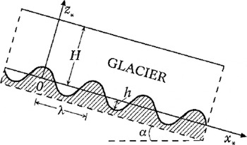
Let the ice be a Newtonian viscous fluid of constant density ρ moving down a sloping plane. The mean inclination angle with respect to the horizontal is α. The sloping plane has sinusoidal corrugations with height h and wavelength λ. The layer thickness in the undisturbed state is constant and equal to H. The motion is two-dimensional and will be described in a Cartesian coordinate system, where the x _* axis is directed along the undisturbed bottom. The z _* axis is taken to be perpendicular to this direction and positive upwards (see Fig. 1). The bottom topography is given by

(1)

Fig. 1. Sketch of the investigated glacier-flow geometry.

We scale our length by H, time by H² /v, velocity by v/H and the pressure per unit density by v² /H² , where v is the kinematic viscosity coefficient. We will apply a Lagrangian description of motion, and write the non-dimensional displacement field (X, Z) = (x _*, z_* )/H and the pressure Π per unit density as (Reference PiersonPierson, 1962)

(2)

where (a, c) can be considered as initial, non-dimensional particle coordinates, constituting the Lagrangian variables, and where t denotes non-dimensional time. Furthermore, Π₀ is a constant and G = gH³ cos α/v² , where g is the acceleration due to gravity. We consider here slow motion of a very viscous fluid, and we write for the conservation of momentum and volume in this case (Reference WeberWeber, 1983)

(3)

where ∇V_L ² = ∂²/∂a ² + ∂²/∂c ² is the linear part of the Laplacian operator. Furthermore, J is the Jacobian defined

by

(4)

and N is the non-linear part of the Laplacian operator given by

(5)

In Equation (3) we have defined

(6)

which is the relevant Reynolds number for the present problem. In our Lagrangian formulation the bottom ice boundary is always situated at c = 0, while the surface is located at c = 1. The bottom topography given by Equation (1) can now be written as

(7)

where ∊ = h/H and k = 2πH/λ are the non-dimensional corrugation amplitude and wavenumber, respectively.

At the bottom we assume a no-slip condition, i.e.

(8)

The surface of the glacier is free to move. Here we assume that the stresses in the along-slope and cross-slope directions are zero, i.e. we neglect the dynamic effect of air above the ice. With the large differences in viscosity between ice and air in mind, this seems to be a reasonable assumption. The Lagrangian form of the stress-free conditions at the surface will be stated when necessary. We finally remark that the Reynolds number (Equation (6)), arising from scaling arguments, equivalently may be written as R = VH/v, where V = gH ² sin α/v is twice the surface velocity for flat-bottom, viscous-slope flow with a stress-free top.

Solutions for the Flow Field

Glacial flows are characterized by very small Reynolds numbers. In addition, we take the non-dimensional bottom corrugation amplitude ∊ = h/H to be much less than one, which is often assumed in analyses of this kind (e.g. Reference MorlandMorland, 1976a, b). Accordingly, if we write the solutions as series expansions after R and ∊ (Reference Weber and DebernardWeber and Debernard, 2000), we can expect the series to converge quite rapidly. Hence

(9a)

(9b)

(9c)

In applying this procedure to glacial flow, where R typically is in the range 10⁻¹¹ to 10⁻¹⁷ (Reference NyeNye, 1969), it is obvious that we do not have to consider terms involving higher orders than R ¹. This is equivalent to making the creeping-flow assumption, i.e. neglecting the convective acceleration in the Eulerian description.

At the bottom, the no-slip condition (Equation (8)) prevents the along-slope displacements from increasing in time. Therefore, the displacement x at c = 0 can be assumed to be small. We can then write the cross-slope displacement (Equation (7)) at the wavy bottom as

(10)

Inserting x from Equation (9a) into Equation (10), we obtain, by comparison with Equation (9b), that the geometrical constraints for the cross-slope displacement to the various orders at the bottom c = 0 become

(11)

etc. Here we have utilized x ⁽¹⁰⁾(c = 0) = 0 (no-slip bottom). These results presuppose that R ≪ 1 and ∊ ≪ 1. Furthermore, the corrugation wave steepness ∊_k must be less than unity.

To O(R ¹ ∊ ⁰) we have z ⁽¹⁰⁾ = 0 at the lower boundary, so there is no along-slope variation to this order. Introducing for brevity u ₀ = x_t ⁽¹⁰⁾ we obtain from Equation (3) for steady flow

(12)

where we have defined D = d/dc. The no-slip and free-slip conditions at the bottom and top, respectively, are stated as

(13)

The solution to this order is the free-surface plane Poiseuille flow given by

(14)

Furthermore, z ⁽¹⁰⁾ = π ⁽¹⁰⁾ = 0 everywhere.

To O(R ⁰ ∊ ¹) the momentum equation yields that the displacement field has no vorticity. For a steady state, the balance in the vertical is purely hydrostatic, i.e. π ⁽⁰¹⁾ = −Gz ⁽⁰¹⁾. The solution to this order is quite simply the adjustment of volume caused by introduction of the corrugated bottom. It is governed by Equation (3) for the conservation of volume. Utilizing that the vorticity is zero, we can introduce a displacement potential ψ ⁽⁰¹⁾ such that x ⁽⁰¹⁾ = ψ_a ⁽⁰¹⁾ and z ⁽⁰¹⁾ = ψ_c ⁽⁰¹⁾. Volume conservation to this order then implies

(15)

The geometrical constraint (Equation (11)) at the bottom to this order is given by z ⁽⁰¹⁾ = cos k_a at c = 0. Vanishing vertical stress at the upper boundary requires that π ⁽⁰¹⁾ = 0 at c = 1. In terms of the displacement potential this becomes

(16)

Accordingly, from Equations (15) and (16)

(17)

and hence

(18)

For the steady solutions to O(R ⁰ ∊ ²) we must again have hydrostatic balance in the vertical, while conservation of volume to this order requires

(19)

At the bottom we have from Equation (11) for this case that z ⁽⁰²⁾ = −k_x ⁽⁰¹⁾ sin ka at c = 0, while vanishing vertical stress at the upper boundary, utilizing the hydrostatic equation, can be written as z ⁽⁰²⁾ = 0 at c = 1. The solutions now become

(20)

We note here the interesting fact that the average over one wavelength in the Lagrangian space (see the definition in Equation (34)) yields a non-zero, negative value for the mean cross-slope displacement in the ice. This means that for an originally horizontal row of N equally spaced elements a ₁, a ₂, a ₃ … a_N within one wavelength, more elements are displaced downwards than upwards in order to comply with the imposed cosine bottom. However, initially square elements which are displaced upwards will tend to become flat and long, while downward displaced elements will become high and thin. In this way the centre of mass for the system will become unaltered to this order (see Reference Debernard and WeberDebernard and Weber (2000) for a related problem in the limit of large wavenumbers).

The steady solutions for the velocity field to O(R ¹ ∊ ¹) are obtained from

(21)

where we have only stated the non-zero contributions to the righthand sides. Defining

(22)

we finally obtain from Equation (21) that

(23)

The solution becomes

(24)

where K ₁, K ₂, K ₃, K ₄ are integration constants. The no-slip condition for the velocity at the bottom yields to this order

(25)

Assuming a steady surface shape (z_t ⁽¹¹⁾ = 0) and a vanishing along-slope surface stress, we find at the upper boundary

(26)

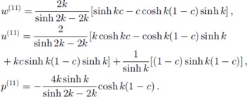
The four conditions in Equations (25) and (26) determine the constants in Equation (24), and the solutions to this order can be written

(27)

The steady surface shape to this order is obtained from the requirement that the cross-slope stress vanishes at the surface. Since x_tc ⁽¹⁰⁾ = 0 at c = 1 (see Equation (13)), this requirement can be written as

(28)

From Equation (28), utilizing Equations (22) and (27), we then obtain for the steady surface elevation

(29)

where

(30)

We note that the surface amplitude function T is always positive. In the present problem the bottom corrugations (Equation (1)) are given in non-dimensional form by

(31)

According to the results above, the steady surface elevation to O(R ¹ ∊ ¹) can be written as

(32)

where we have utilized the fact that R/G = tan α, which is the mean bottom slope. The function T(k) tan a is called the transfer function. From Equation (30) we realize that the transfer function tends to infinity when k → 0. This is related to our adopted boundary condition w ⁽¹¹⁾ = 0 at the free surface, which was introduced to simplify the solutions to O(R ¹ ∊ ¹). To have a physically acceptable solution, we must require T(k) < cot α. This poses a lower limit for k when α is given. Assuming that this limit is attained for small k, we find from Equation (30) that k > 3 tan α. Accordingly, for naturally occurring slopes, it appears that the present theory is valid at least for wavelengths up to ten times the glacier depth.

From Equations (31) and (32) we realize that the surface undulation is 90° out of phase with the bottom corrugations. However, this is not a general result. It is valid when w ⁽¹¹⁾ = 0 at the free surface, as we have assumed here. Computations of the shape of the free surface when ice flows over topography go back to Reference YosidaYosida (1964) and Reference BuddBudd (1970). Their analyses have been improved (see Reference HutterHutter, 1983). However, for a linear ice rheology with a no-slip bottom and non-vanishing normal velocity at the surface, Reference ReehReeh (1987) appears to be the first to have analyzed this problem correctly, using linear perturbation theory. The general case, allowing for slip at the bed, yields rather complicated transfer functions (e.g. Reference Balise and RaymondBalise and Raymond, 1985; Reference JóhannessonJóhannesson, 1992; Reference Gudmundsson, Raymond and BindschadlerGudmundsson and others, 1998).

In the present paper we focus on the non-linear effect of the bottom corrugations, and in particular how they alter the mean particle velocity. To keep the computational efforts to a minimum, we have neglected the normal velocity to O(R ¹ ∊ ¹) at the free surface. This means that our analysis is not valid for very long wavelengths, as discussed above.

Mean Steady-State Particle Velocity

To obtain a correction to the basic Poiseuille flow (Equation (14)) with a mean that is different from zero, we have to proceed to O(R ¹ ∊ ¹). Introducing Lagrangian averages, the equation for steady flow along the slope can be written from Equation (3) to this order as

(33)

The overbar is defined by

(34)

representing the Lagrangian mean. In Equation (33) we have written down only terms that yield non-zero contributions to the righthand side. Mathematically, the solution to this steady problem is not unique. For example, a solution with a mean constant glacier depth is perfectly possible. However, such a solution will yield a reduction of the total, mean volume flux above the corrugations. If there is no change in the accumulation rate far upstream, it is physically reasonable to assume that the total ice-volume flux should be unaltered by the introduction of the sinusoidal bottom corrugations. This requires an external mean pressure gradient to O(R ¹ ∊ ¹) which induces a flow that balances, in a volume flux sense, the flow induced by the corrugations. Reference Weber and TyvandWeber (1997) considers a similar case when ocean waves induce a mean particle drift towards the shore, and where mass balance requires a mean sloping ocean surface. Accordingly, we assume in Equation (33) that the mean, external dynamic pressure gradient can be written as

(35)

where γ is a constant. At the free surface, we have . Hence we obtain for the mean surface slope to O(R ¹ ∊ ¹):

(36)

As explained above, the constant γ must be determined such that the perturbation volume flux is zero, i.e.

(37)

By inserting the various orders in Equation (33), we finally obtain

(38)

where we have defined and

(39)

By substituting our solutions to the various orders into the condition for zero along-slope stress at the upper boundary, and taking the mean, we obtain to this order that the mean Lagrangian shear must vanish there, i.e. Du ₂ = 0 at c = 1. Furthermore, utilizing the no-slip condition u ₂ = 0 at c = 0, we obtain from Equation (38) for the mean particle drift to O(R ¹ ∊ ¹) that

(40)

From Equations (37) and (40) we finally obtain

(41)

It is straightforward to find the asymptotic formulae for the mean particle velocity (Equation (40)) when the non-dimensional wavenumber k is small or large. For k ≪ 1, we obtain u ₂ → 0. We here recall the requirement that k > 3 tan α for the O(R ¹ ∊ ¹) solution to be valid (see the discussion related to Equation (32)). When k ≫ 1, Equation (40) reduces to

(42)

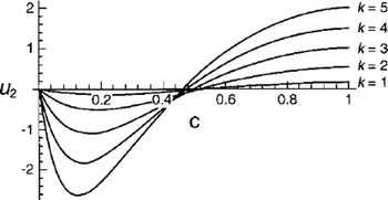
We find here a positive value for the flow in the upper part of the layer, and a negative boundary-layer jet of thickness 1/(2k) close to the wavy ground. The asymptotic formula (Equation (42)) reveals the basic feature of the general solution for arbitrary k. The first term on the righthand side corresponds to the Poiseuille flow driven by the mean surface tilt, and is always directed downslope. The second term is the mean mass transport velocity that is generated by the nonlinear interaction between the basic shear flow and the bottom corrugations. This part of the flow is always directed upslope. We notice the same features from Figure 2, where we have plotted u ₂ as function of height for various values of k.

Fig. 2. Induced mean drift u₂ from Equation (40) vs Lagrangian height c for various values of k.

It is tempting to speculate that the total mean particle velocity in some cases even may be directed upslope near the bottom since the basic Poiseuille flow here is small. For example, the total along-slope mean particle velocity u/R = u ₀ + ∊ ² u ₂ from Equations (14) and (40) is upslope near the ground when k = 9 and ∊ = 0.1. In fact, for k ≫ 1, we find from Equations (14) and (42) that Du(c = 0) < 0, i.e. upslope flow near the ground, when . However, restrictions on the non-dimensional corrugation amplitude ∊ and the wave steepness ∊_k , which both must be less than unity, force us to treat such cases with care. Future numerical solutions of the governing equations and/or laboratory experiments can eventually verify the validity of the results in this parameter regime.

Bottom Drag

When sinusoidal corrugations are introduced into a constant shear flow (Couette flow), the mean bottom drag increases (Reference WangWang, 1978). In the present problem, the motion is basically driven by the action of gravity. With vanishing stresses at the free surface and no external along-slope pressure gradients, i.e. γ = 0 in Equation (40), the introduction of sinusoidal bottom corrugations does not alter the mean bottom drag (Reference MorlandMorland, 1976a), because the mean position of the centre of mass is not changed by the introduction of periodic bottom undulations. The drag can simply be obtained from the shear of the Poiseuille profile (Equation (14)) at c = 0. When we introduce a constant, external dynamic pressure gradient γ (<0) into this problem to ensure that the perturbation ice-volume flux is zero (see Equation (36)), the mean bottom drag is increased by the factor R∊ ²|γ|.

A Digression on Shear Heating

In this analysis of glacier flow we have taken the density and the viscosity to be independent of temperature and pressure. This appears to be a fair assumption for a non-temperate glacier as far as the fluid mechanical part is concerned. However, we would like to discuss briefly some consequences our results may have for the heat flow in the glacier. In glaciers that are frozen to the ground, the velocity shear becomes much stronger than when sliding occurs. We therefore expect the effect of shear heating (e.g. Reference Yuen and SchubertYuen and Schubert, 1979), to be more important for non-temperate glaciers than for temperate, sliding glaciers. In the present paper we look at the existence of the bottom corrugations as perturbations on a basic state which is uniform in the along-slope direction. The basic flow field is given by Equation (14), and the basic vertical temperature distribution is governed by the geothermal heat flux at the base, the shear heating within the ice and the temperature, say, at the top of the ice. For the simplified case of a Newtonian viscous fluid with constant viscosity and heat diffusivity, the basic temperature distribution in the ice is readily obtained from the results of Reference Yuen and SchubertYuen and Schubert (1979).

The response times for the velocity perturbations and the temperature perturbations are very different for a glacier. A velocity perturbation will be felt through the entire ice layer in a characteristic diffusion time proportional to H ²/ν, which is extremely small due to the very large value of the kinematic viscosity. More accurately, a velocity change will diffuse through a semi-infinite medium in the mathematical form of the complementary error function of argument , where r is the dimensional length coordinate (e.g. Reference Carslaw and JaegerCarslaw and Jaeger, 1959). For ν = 3.5 × 10⁹ m² s⁻¹ (Reference NyeNye, 1969), a velocity change will manifest itself at a distance of 200 m from the base in <1 s. Similarly, a temperature perturbation has a characteristic diffusion time proportional to H ²/k, where k is the thermal diffusivity. The value of k for ice is close to 10⁻⁶ m² s⁻¹. Accordingly, it will take a temperature change hundreds of years to diffuse through the glacier. Therefore, the velocity shear and the associated dissipation induced by the undulating ground will appear almost instantaneously as a heat source in the equation for the perturbation temperature. In general we have for the dissipation Q in the two-dimensional, non-divergent, viscous Newtonian approximation that

(43)

where u and w are the dimensionless Eulerian velocity components in the x _* and z _* directions, respectively. By transforming to Lagrangian variables (e.g. Reference LambLamb, 1932), the perturbation dissipation q induced by the bottom corrugations can be written to lowest order as

(44)

Here we have defined

(45)

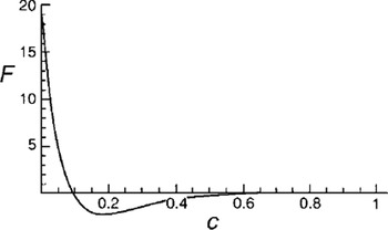
where u ⁽¹¹⁾ and w ⁽¹¹⁾ are given by Equation (27). For large values of k the dissipation amplitude F has a typical boundary-layer structure with large values near the base (see Fig. 3, where we have plotted F vs height for k = 10). We therefore concentrate on the heat production at the base (c = 0) of the glacier. For small times we may neglect the effect of heat diffusion. The rate of change for the perturbation temperature θ at the ground, where the velocity is zero, can then be written in dimensional form

(46)

Fig. 3. The dissipation amplitude F from Equation (45) vs height for k = 10.

Here c _i is the specific heat capacity for ice. By inserting q from Equation (44), we obtain for the perturbation temperature at the base of the glacier

(47)

valid for small times. Here we have inserted the Reynolds number R (Equation (6)), and defined

(48)

We find that F ₀ increases monotonically with k, such that F ₀ = 2 when k = 0, and F ₀ → 2k when k ≫ 1. Since the bottom topography (Equation (31)) and the perturbation temperature (Equation (47)) both have a cosine variation along the slope, the shear heating produces a temperature increase at the wave crests and a temperature decrease at the troughs along the ground. Choosing c _i = 2 × 10 J kg⁻¹ K⁻¹, α = 33.5° (Reference Yuen and SchubertYuen and Schubert, 1979), v = 3.5 × 10⁹ m² s⁻¹ (Reference NyeNye, 1969) and H = 200 m, we find for large wavenumbers and ∊k = 0.5 that the perturbation temperature (Equation (47)) at a crest (X = 0) becomes

(49)

Accordingly, within 12 days the temperature may have increased by about 0.4^oC at a wave crest. At that time, heat diffusion will typically have influenced length scales of order 1–2 m, so the shear heating at small times will be confined to the region close to the crest at the base. Hence, in cases where the base temperature is close to but below the melting temperature, we may expect that corrugation-induced shear heating might cause melting at the wave crests along the sloping bottom (changes of the melting point caused by the pressure perturbations are negligible in this context). Then a lubricating water layer may form here, which means that the no-slip condition will be violated and sliding may occur. Because of the very fast response time for momentum changes in the ice, the increased velocity due to slipping will quickly be felt through the entire ice column, and along-slope convergencies and divergencies in the flow field may develop. For glaciers the associated large strain rates could in turn lead to the formation of crevasses in the divergent zones between the frozen troughs and the lubricated crests. A similar crevassing has been reported in cases where the upper part of the glacier is frozen to the ground and the lower part can slide (Reference Lliboutry, Briat, Creseveur and PourchetLliboutry and others, 1976).

Our calculated value for the local temperature rise has been obtained for a rather steep sloping ground. It should be noted from Equation (47) that for more moderate slopes, similar increases may occur near wave crests under thicker glaciers or ice sheets.

Summary and Concluding Remarks

We have studied the flow of a glacier over wavy sloping ground as a non-linear interaction problem between a basic flow and the bottom corrugations. This is achieved by utilizing a Lagrangian description of motion. A Newtonian viscous approximation is used for the ice. The resulting interaction current, averaged over one wavelength, is always directed upslope. To ensure ice-volume flux balance, a surface-tilt driven flow must be added that is always directed downslope. In this way the mean particle perturbation velocity becomes directed upslope near the wavy ground and downslope in the upper part of the glacier.

The use of a direct Lagrangian approach for studying glacier flow seems not to have been reported in the literature before. This approach is often preferable to the more traditional Eulerian description in studies of non-linear mass transport associated with periodic disturbances (e.g. Reference Weber and TyvandWeber, 1997). In particular, the Eulerian analysis usually fails to yield the Stokes-drift part of the flow. The use of a Lagrangian description is not restricted to Newtonian viscous fluids. It could also be a valuable tool for analyzing glacier flow over topography with a more complex ice rheology.

Acknowledgement

The author is indebted to G. H. Gudmundsson for helpful comments on the manuscript.