


1. Introduction
It is well known that turbulent wall-bounded flows of high molecular weight polymer solutions can have significantly less skin-friction drag than Newtonian fluids at a similar Reynolds number. Since its discovery by Toms (Reference Toms1948), the phenomenon of polymer drag reduction (DR) has garnered considerable attention (Lumley Reference Lumley1969; Procaccia, L'vov & Benzi Reference Procaccia, L'vov and Benzi2008; White & Mungal Reference White and Mungal2008; Graham Reference Graham2014; Xi Reference Xi2019); yet, the fundamental question of how polymers reduce drag remains elusive. An incomplete understanding of the mechanism of DR can be attributed to the complexity of the turbulent flow, coupled with the complexity of the polymer solution and its non-Newtonian constitutive equation (White & Mungal Reference White and Mungal2008). Revealing the mechanics of polymer DR requires comparisons between experiments that accurately measure the fluctuating velocity field of polymer drag-reduced wall flows, and numerical simulations that utilize non-Newtonian constitutive models. Antiquated works generally involved interpretations of various ensemble statistics, such as mean velocity and Reynolds stresses. While the focus of more recent investigations has shifted towards understanding the distribution and evolution of coherent flow structures – an analysis propelled almost entirely by works using numerical simulations (Xi Reference Xi2019). Experiments have trailed in this regard, most likely due to the tremendous difficulties involved with measuring coherent structures. Therefore, the broad goal of the present investigation is to determine the three-dimensional (3-D) topology of the turbulent motions within a polymer-laden boundary layer using modern flow measurements.
There are several methods for identifying the topology of the turbulent motions. The present work utilizes that of Chong, Perry & Cantwell (Reference Chong, Perry and Cantwell1990), herein referred to as the  $\varDelta$-criterion, where $\varDelta$ is defined as the discriminant of the characteristic equation for the velocity gradient tensor (VGT). The $\varDelta$-criterion utilizes the eigenvalues and invariants of the VGT to identify the local topology and streamline patterns about critical points within the flow. Examples of flow topologies include those that are focal (vortical) and dissipative (saddle points), depending on the sign of the invariants and the real/complex nature of the eigenvalues. Using the $\varDelta$-criterion, various works have demonstrated that quasi-streamwise and hairpin vortices can be visualized in numerical simulations and flow measurements of Newtonian wall-bounded turbulence (Blackburn, Mansour & Cantwell Reference Blackburn, Mansour and Cantwell1996). Furthermore, the joint probability density function (j.p.d.f.) of the invariants in the VGT takes on a tear-drop or pear-shaped distribution. This tear-drop pattern in the j.p.d.f. of the VGT invariants is not only found in wall-bounded turbulence (Blackburn et al. Reference Blackburn, Mansour and Cantwell1996; Chacín, Cantwell & Kline Reference Chacín, Cantwell and Kline1996; Chong et al. Reference Chong, Soria, Perry, Chacín, Cantwell and Na1998; Chacín & Cantwell Reference Chacín and Cantwell2000; Elsinga & Marusic Reference Elsinga and Marusic2010), but also turbulent mixing layers (Soria et al. Reference Soria, Sondergaard, Cantwell, Chong and Perry1994; Buxton, Laizet & Ganapathisubramani Reference Buxton, Laizet and Ganapathisubramani2011), jets (da Silva & Pereira Reference da Silva and Pereira2008; Buxton & Ganapathisubramani Reference Buxton and Ganapathisubramani2010) and isotropic turbulence (Martın et al. Reference Martın, Ooi, Chong and Soria1998; Ooi et al. Reference Ooi, Martin, Soria and Chong1999; Danish & Meneveau Reference Danish and Meneveau2018), implying a universal distribution of topologies exists among different types of Newtonian turbulence.
Few investigations have used the  $\varDelta$-criterion to explore the distribution of flow topologies in wall-bounded turbulence with non-Newtonian rheology (Mortimer & Fairweather Reference Mortimer and Fairweather2022). The work by Mortimer & Fairweather (Reference Mortimer and Fairweather2022) observed an unambiguous change in the topology of a viscoelastic channel flow at a friction Reynolds number $Re_{\tau }$ of 180, and derived from direct numerical simulation (DNS) utilizing the FENE-P constitutive model. Here, FENE-P stands for finitely extensible nonlinear elastic dumbbells with the Peterlin approximation. Mortimer & Fairweather (Reference Mortimer and Fairweather2022) demonstrated that drag-reduced channel flows have a narrower range in the third invariant of the VGT and flow structures were more two dimensional, relative to Newtonian channel flows at a similar $Re_{\tau }$. Despite these observations, the flows investigated by Mortimer & Fairweather (Reference Mortimer and Fairweather2022) had very low DR percentages (less than 5 %) and modest non-Newtonian rheology, with negligible shear thinning and relatively low amounts of elasticity compared with other numerical investigations of drag-reduced flows (Xi Reference Xi2019). Therefore, it is unclear what the topology based on the $\varDelta$-criterion would look like for flows with larger amounts of DR, let alone a flow that utilizes a realistic polymer solution that is shear thinning and viscoelastic.
While the  $\varDelta$-criterion has not been employed to investigate the topology of polymer drag-reduced flows with large amounts of DR, it has been used to assess the topology of low-Reynolds-number transitional channel flows exhibiting elasto-inertial turbulence (EIT). Samanta et al. (Reference Samanta, Dubief, Holzner, Schäfer, Morozov, Wagner and Hof2013) observed that below the critical Reynolds number for laminar-turbulent transition, polymer-laden pipe and channel flows exhibit an early transition to a different type of disordered motion referred to as EIT. Numerical simulations of channel flows utilizing the FENE-P constitutive model have demonstrated that EIT is inherently two dimensional and consists of alternating regions of vortical and dissipative flow (i.e. positive and negative $\varDelta$) along the streamwise direction (Samanta et al. Reference Samanta, Dubief, Holzner, Schäfer, Morozov, Wagner and Hof2013). In the j.p.d.f. of the VGT invariants, EIT reflects a symmetric ovular pattern that is significantly different than the tear-drop pattern observed in Newtonian turbulence (Dubief, Terrapon & Soria Reference Dubief, Terrapon and Soria2013). The connection between EIT and DR, and whether it persists at much larger Reynolds numbers, is still unknown (Xi Reference Xi2019). Therefore, comparing the measured topology of a polymer drag-reduced flow with the known topology of EIT derived from viscoelastic simulations could provide evidence that EIT contributes to the dynamics at larger Reynolds numbers.
Although few works have used the  $\varDelta$-criterion to characterize the topology of polymer drag-reduced flows, observations of coherent structures have been performed using other techniques. For example, Pereira et al. (Reference Pereira, Mompean, Thais and Thompson2017) utilized a modified $Q$-criterion, or the second invariant in the VGT (Hunt, Wray & Moin Reference Hunt, Wray and Moin1988; Martins et al. Reference Martins, Pereira, Mompean, Thais and Thompson2016), to discern vortical and extensional structures in channel flow DNS with the FENE-P constitutive model, an $Re_{\tau }$ between 180 and 1000, and DR as large as 62 %. Pereira et al. (Reference Pereira, Mompean, Thais and Thompson2017) noted that both extensional and vortical flow motions in the drag-reduced channel flow were weaker relative to Newtonian DNS, and the flow tended towards a more parabolic (shear-dominant) state – a trend Pereira et al. (Reference Pereira, Mompean, Thais and Thompson2017) referred to as ‘flow parabolization’. An earlier investigation by Roy et al. (Reference Roy, Morozov, van Saarloos and Larson2006) similarly implied flow parabolization based on channel flow simulation that utilized a simplified constitutive model of polymer stresses (the retarded-motion expansion). Roy et al. (Reference Roy, Morozov, van Saarloos and Larson2006) more specifically asserted that the non-Newtonian extensional viscosity opposed flow in both uniaxial and biaxial flow regions, thus mitigating the strength and formation of quasi-streamwise vortices and reducing drag. Many of the previously listed numerical investigations (Roy et al. Reference Roy, Morozov, van Saarloos and Larson2006; Pereira et al. Reference Pereira, Mompean, Thais and Thompson2017; Mortimer & Fairweather Reference Mortimer and Fairweather2022) provide meaningful assertions about the influence of polymer rheology on flow topology; however, all of these works utilize constitutive models, such as FENE-P, that only approximate polymer-driven stresses (Xi Reference Xi2019) and few experiments have measured the topology of a polymer drag-reduced flow to corroborate these observations.
Early experimental investigations made inferences about the size of large-scale motions in polymer drag-reduced flows based on measurements using two-dimensional (2-D) particle image velocimetry (PIV) and two-point velocity statistics. One such notable experimental work was that of White, Somandepalli & Mungal (Reference White, Somandepalli and Mungal2004), which investigated a drag-reduced boundary layer with near-wall injection of a concentrated polymer solution, a momentum thickness-based Reynolds number  $Re_{\theta }$ of 1300 to 1400 and DR between 33 % and 67 %. Within the buffer layer of the flow, White et al. (Reference White, Somandepalli and Mungal2004) observed visibly wider and longer high- and low-speed velocity streaks for a flow with DR of 50 % relative to water at a similar $Re_{\theta }$. Two-point spatial correlations of the streamwise velocity fluctuations along the spanwise direction confirmed that the large-scale motions became increasingly wider as DR grew from 33 % to 67 %. A similar widening and elongation of the large-scale motions was observed for drag-reduced boundary layers of homogeneous polymer solutions (often referred to as a polymer ocean) by Farsiani et al. (Reference Farsiani, Saeed, Jayaraman and Elbing2020), and also homogeneous polymer drag-reduced channel flows by Warholic et al. (Reference Warholic, Heist, Katcher and Hanratty2001) and Warwaruk & Ghaemi (Reference Warwaruk and Ghaemi2021). In addition to velocity correlations, White et al. (Reference White, Somandepalli and Mungal2004) also observed a reduction in the strength and number of near-wall vortices, albeit inferred from visualization of an instantaneous snapshot of the wall-normal vorticity. From an experimental perspective, the natural progression to the work of White et al. (Reference White, Somandepalli and Mungal2004) is to better quantify the near-wall vortical structures of a polymer drag-reduced flow using 3-D flow measurements and a suitable method for detecting such structures.
A limited number of experimental investigations have used 3-D flow measurements to measure the velocity in polymer drag-reduced flows, let alone one that quantifies the topology of fine-scale motions within the flow. Shah, Ghaemi & Yarusevych (Reference Shah, Ghaemi and Yarusevych2021) performed 3-D tomographic PIV on a polymer drag-reduced boundary layer with heterogeneous wall injection, an  $Re_{\theta }$ of 520 and DR of 20 %–30 %. Using a modified $Q$-criterion (Hunt et al. Reference Hunt, Wray and Moin1988; Martins et al. Reference Martins, Pereira, Mompean, Thais and Thompson2016), Shah et al. (Reference Shah, Ghaemi and Yarusevych2021) demonstrated that extensional and vortical flow regions weaken as drag was reduced, similar to the findings of the numerical investigation by Pereira et al. (Reference Pereira, Mompean, Thais and Thompson2017). Rather than $Q$-criterion, the current work expands on the experimental findings of Shah et al. (Reference Shah, Ghaemi and Yarusevych2021) by utilizing the $\varDelta$-criterion to obtain distributions, mainly j.p.d.f.s, of the different types of topologies within a Newtonian and polymer-laden turbulent boundary later (TBL). Compared with the $Q$-criterion, use of the $\varDelta$-criterion, as well as other deformation tensor invariants, facilitates a more complete depiction of the topology of fine-scale motions within the turbulent drag-reduced flow. Unlike the use of just $Q$, considering the other tensor invariants and $\varDelta$ can help distinguish structures that are in uniaxial or biaxial extension, as well as focal or dissipative; some of which are significant to the mechanism for polymer DR.
In the present investigation, the VGT of a polymer drag-reduced boundary layer will be measured using state-of-the-art 3-D particle tracking velocimetry (3-D-PTV), from which the local flow topology will be analysed using the  $\varDelta$-criterion. Evidence is provided to test a hypothesis regarding the mechanism of polymer DR. This hypothesis is inspired by the works of Roy et al. (Reference Roy, Morozov, van Saarloos and Larson2006) and Lumley (Reference Lumley1973) – that being, the large extensional viscosity of polymer solutions strongly inhibits uniaxial and biaxial flow regions, thus mitigating the strength and formation of quasi-streamwise vortices and reducing drag. It is clear that even small amounts of DR will produce an unambiguous change in the topology of a TBL (Pereira et al. Reference Pereira, Mompean, Thais and Thompson2017; Mortimer & Fairweather Reference Mortimer and Fairweather2022); however, based on the findings of Roy et al. (Reference Roy, Morozov, van Saarloos and Larson2006), it is expected that changes in the topology will predominately occur in regions of strong uniaxial/biaxial extension. Uniaxial/biaxial flow regions are dissipative with $\varDelta <0$, and are strongly concentrated around the ‘tails’ in the j.p.d.f. of the VGT invariants. They can also be identified from the invariants in the rate of deformation tensor (RDT) or the symmetric component of the VGT, which will be elaborated upon more in § 2 to follow.
2. Theoretical background
The following section will serve to summarize the  $\varDelta$-criterion of Chong et al. (Reference Chong, Perry and Cantwell1990). This method utilizes the eigenvalues and invariants of the VGT to identify the local topology and streamline patterns of the flow. The VGT is $\boldsymbol{\mathsf{L}} = \boldsymbol {\nabla } \boldsymbol {U}$ and $\boldsymbol {U}$ is the velocity vector. The characteristic equation for the tensor $\boldsymbol{\mathsf{L}}$ is
 \begin{equation} \varLambda^3 + P \varLambda^2 + Q \varLambda + R = 0, \end{equation}
 where  $P$,
$P$,  $Q$ and $R$ are the invariants of $\boldsymbol{\mathsf{L}}$. The eigenvalues are the roots to (2.1), and are defined as $\varLambda _1$, $\varLambda _2$ and $\varLambda _3$ in descending order of magnitude. Although the $\varDelta$-criterion can be applied to both compressible and incompressible fluid flows, the present work focuses only on those that are incompressible, thus narrowing down the number of flow classifications. In an incompressible flow, the first invariant $P = -\mathrm {tr}(\boldsymbol{\mathsf{L}})$ is equal to zero, while $Q$ and $R$ are the only non-zero invariants of $\boldsymbol{\mathsf{L}}$ and can be expressed as
 $$\begin{gather} Q =-\tfrac{1}{2}\mathrm{tr}(\boldsymbol{\mathsf{L}}^2), \end{gather}$$
 $$\begin{gather}R =-\mathrm{det}(\boldsymbol{\mathsf{L}}). \end{gather}$$
Here,  $\mathrm {tr}(\dots )$ represents the trace operator on a square matrix and $\mathrm {det}(\dots )$ the determinant. The nature of the eigenvalues of $\boldsymbol{\mathsf{L}}$ are dictated by the sign convention of the discriminant $\varDelta$ of (2.1),
 \begin{equation} \varDelta = \tfrac{27}{4}R^2 + Q^3, \end{equation}
where  $\varDelta >0$ produces one real and two complex eigenvalues, and $\varDelta \leq 0$ produces three real eigenvalues. Figure 1 describes the different possible local flow topologies that depend on the sign convention of $\varDelta$ and $R$ (Chong et al. Reference Chong, Perry and Cantwell1990). The lines corresponding to $\varDelta = 0$, and shown in figure 1, are referred to as the Vieillefosse tail's. Here, ( $\varDelta = 0$, $R< 0$) is the left-Vieillefosse tail and ( $\varDelta = 0$, $R>0$) is the right-Vieillefosse tail. Flow conditions above the Vieillefosse tail's with $\varDelta >0$, consist of motions that are focal and primarily vortical. Regions of the flow with $\varDelta \leq 0$ take on a node-saddle-saddle streamline pattern. Flow topology is also divided about the $R=0$ axis, where flows with $R<0$ are stable (stretching) and $R>0$ are unstable (compressing). The j.p.d.f.s of $Q$ and
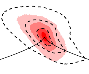
  $R$ in various Newtonian turbulent flows take on a tear-drop pattern (Soria et al. Reference Soria, Sondergaard, Cantwell, Chong and Perry1994; Blackburn et al. Reference Blackburn, Mansour and Cantwell1996; Chong et al. Reference Chong, Soria, Perry, Chacín, Cantwell and Na1998; Ooi et al. Reference Ooi, Martin, Soria and Chong1999; da Silva & Pereira Reference da Silva and Pereira2008). The point or tip of the tear-drop falls on the right-Vieillefosse tail ( $\varDelta = 0, R>0$), while the bulb of the tear drop is situated in the quadrant of stable focus stretching ( $\varDelta >0, R<0$).

Figure 1. Local topologies for different  $R$ and $Q$ in an incompressible flow with $P=0$ (Chong et al. Reference Chong, Perry and Cantwell1990).
The VGT indicated as  $\boldsymbol{\mathsf{L}}$ can be separated into a symmetric and antisymmetric component, where $\boldsymbol{\mathsf{L}} = \boldsymbol{\mathsf{D}} + \boldsymbol{\mathsf{W}}$. Here the symmetric RDT is $\boldsymbol{\mathsf{D}} = (\boldsymbol {\nabla } \boldsymbol {U} + \boldsymbol {\nabla } \boldsymbol {U}^{{\dagger} })/2$, the antisymmetric rate of rotation tensor (RRT) is $\boldsymbol{\mathsf{W}} = (\boldsymbol {\nabla } \boldsymbol {U} - \boldsymbol {\nabla } \boldsymbol {U}^{{\dagger} })/2$, and the dagger symbol ${\dagger}$ represents the matrix transpose. Similar to $\boldsymbol{\mathsf{L}}$, the tensors $\boldsymbol{\mathsf{D}}$ and $\boldsymbol{\mathsf{W}}$ have their own characteristic equation. For the tensor $\boldsymbol{\mathsf{D}}$, the characteristic equation is
 \begin{equation} \varGamma^3 + P_D \varGamma^2 + Q_D \varGamma + R_D = 0, \end{equation}
where  $P_D = -\mathrm {tr}(\boldsymbol{\mathsf{D}}) = 0$ for an incompressible flow, and the non-zero invariants are defined according to
 $$\begin{gather} Q_D =-\tfrac{1}{2}\mathrm{tr}(\boldsymbol{\mathsf{D}}^2), \end{gather}$$
 $$\begin{gather}R_D =-\mathrm{det}(\boldsymbol{\mathsf{D}}) =-\tfrac{1}{3} \mathrm{tr}(\boldsymbol{\mathsf{D}}^3). \end{gather}$$
The roots of (2.4) are the eigenvalues of  $\boldsymbol{\mathsf{D}}$ and are defined as $\varGamma _1$, $\varGamma _2$ and $\varGamma _3$ in descending order of magnitude. Similar to (2.3) for $\boldsymbol{\mathsf{L}}$, the discriminant of (2.4) for $\boldsymbol{\mathsf{D}}$ is
 \begin{equation} \varDelta_D = \tfrac{27}{4}R_D^2+Q_D^3. \end{equation}
 Because  $\boldsymbol{\mathsf{D}}$ is a real and symmetric tensor, its eigenvalues will always be real and $\varDelta _D \leq 0$. A plot of $Q_D$, $R_D$ space is shown in figure 2, where black solid lines represent curves with the same ratio of principal strain rates or eigenvalue of $\boldsymbol{\mathsf{D}}$, defined as $\varGamma _1:\varGamma _2:\varGamma _3$ (Blackburn et al. Reference Blackburn, Mansour and Cantwell1996). The ratio of principal strains are also used to distinguish possible rheometric flows, e.g. uniaxial extension, biaxial extension, planar extension and shear. A review of these basic rheometric flows is not presented, however deriving their respective invariants in $\boldsymbol{\mathsf{D}}$ and $\boldsymbol{\mathsf{W}}$ is trivial; see e.g. pp. 73–75 of Macosko (Reference Macosko1994). The different rheological flows are labelled on the schematic of $R_D, Q_D$ space of figure 2. Uniaxial and biaxial extensions correspond to the lines where $\varDelta _D = 0$. Uniaxial extension flows have an eigenvalue ratio of $\varGamma _1:\varGamma _2:\varGamma _3 = 2:-1:-1$ (i.e. negative $R_D$ and $\varDelta _D = 0$), while biaxial extensional flows have an eigenvalue ratio of $\varGamma _1:\varGamma _2:\varGamma _3 = 1:1:-2$ (positive $R_D$ and $\varDelta _D = 0$). Shear and planar extension both exist on the $R_D=0$ axis and are 2-D flows, with an eigenvalue ratio of $\varGamma _1:\varGamma _2:\varGamma _3 = 1:0:-1$.

Figure 2. Ratios of eigenvalues for different  $R_D$ and $Q_D$ for an incompressible flow with $P=0$. The eigenvalues are listed in the descending order of $\varGamma _1:\varGamma _2:\varGamma _3$ (Blackburn et al. Reference Blackburn, Mansour and Cantwell1996).
Unlike tensors  $\boldsymbol{\mathsf{L}}$ and $\boldsymbol{\mathsf{D}}$, the RRT has only one non-zero invariant by definition, that being the second invariant
 \begin{equation} Q_W =-\tfrac{1}{2} \mathrm{tr}(\boldsymbol{\mathsf{W}}^2). \end{equation}
For any antisymmetric tensor, the determinant is equal to zero; therefore, the third invariant of  $\boldsymbol{\mathsf{W}}$, defined as $R_W$, will always be zero. Also note that the second invariant of $\boldsymbol{\mathsf{L}}$ can be equally represented as $Q = Q_D + Q_W$. Values of $Q_D$ are always negative, while values of $Q_W$ are always positive. The invariants, $Q_D$ and $Q_W$, are also proportional with energy dissipation $\varepsilon = 2\nu \,\mathrm {tr}(\boldsymbol{\mathsf{D}}^2) = -4 \nu Q_D$ and enstrophy density $\phi = -2\,\mathrm {tr}(\boldsymbol{\mathsf{W}}^2) = 4Q_W$, where $\nu$ is the kinematic viscosity. Therefore, the ratio between $Q_W$ and $Q_D$ can indicate whether the flow is more dominated by dissipation or enstrophy. Truesdell (Reference Truesdell1954) established a kinematical vorticity number
 \begin{equation} \mathcal{K} = \left(\frac{Q_W}{-Q_D}\right)^{1/2}, \end{equation}
which defines the local strength of rotation relative to stretching (Ooi et al. Reference Ooi, Martin, Soria and Chong1999). The change in  $\mathcal {K}$ is shown schematically in figure 3 for different $Q_D$ and $Q_W$, similar to the diagram provided in Soria et al. (Reference Soria, Sondergaard, Cantwell, Chong and Perry1994). Regions of the flow with small $Q_W$ and $\mathcal {K} \approx 0$ are more irrotational and dominated by dissipative motions, while flow regions with negligible $Q_D$ and large values of $\mathcal {K}$ that approach $\infty$ experience solid body rotation. Regions with both large enstrophy density and dissipation fall on the line with $\mathcal {K} = 1$, where $Q_W = -Q_D$. From simulations of an incompressible mixing layer, Soria et al. (Reference Soria, Sondergaard, Cantwell, Chong and Perry1994) described how flow motions with $\mathcal {K} = 1$ consist of vortex sheets and shear layers. Comparing the invariants $Q_W$ and $Q_D$ is also commonly used to distinguish rheometric flows. Astarita (Reference Astarita1979) derived a criteria that was adapted from the work of Astarita (Reference Astarita1967), for distinguishing steady shear, extension and solid body rotation in non-Newtonian flows and served functionally the same as the kinematical vorticity number $\mathcal {K}$. Flow regions that are extension dominant ( $\mathcal {K}=0$), shear dominant ( $\mathcal {K}=1$) or in rigid body rotation ( $\mathcal {K}=\infty$) are annotated on the schematic of $Q_D, Q_W$ space shown in figure 3. Dimensionless indicators similar to $\mathcal {K}$ are generally referred to as a ‘flow type’ and can be commonly found in a variety of works involving non-Newtonian flows (Haward, McKinley & Shen Reference Haward, McKinley and Shen2016; Haward, Toda-Peters & Shen Reference Haward, Toda-Peters and Shen2018; Ekanem et al. Reference Ekanem, Berg, De, Fadili, Bultreys, Rücker, Southwick, Crawshaw and Luckham2020; Walkama, Waisbord & Guasto Reference Walkama, Waisbord and Guasto2020; Kumar, Guasto & Ardekani Reference Kumar, Guasto and Ardekani2022).

Figure 3. Schematic of the different flow types in  $Q_W$, $Q_D$ space and for different kinematic vorticity numbers $\mathcal {K}$ (Soria et al. Reference Soria, Sondergaard, Cantwell, Chong and Perry1994).
3. Experimental methodology
The invariants in the VGT of a Newtonian and polymer-laden TBL were computed using velocity vectors measured from 3-D-PTV based on the shake-the-box (STB) algorithm developed by Schanz, Gesemann & Schröder (Reference Schanz, Gesemann and Schröder2016). Newtonian and polymer-laden flows were compared at a similar friction Reynolds number  $Re_{\tau }$ and momentum thickness Reynolds number $Re_{\theta }$. A detailed description of the flow facility, polymer solution, measurement apparatus and flow computations are provided in the following sections.
3.1. Flow facility
Newtonian and polymer-laden TBLs were formed along the floor of a closed-loop water flume at the University of Alberta's Laboratory of Turbulent Flows (Abu Rowin, Hou & Ghaemi Reference Abu Rowin, Hou and Ghaemi2018; Elyasi & Ghaemi Reference Elyasi and Ghaemi2019). The flume consists of a 5 m long channel that bridges two cubic reservoirs. The channel was 0.68 m in width  $W$. The free surface was situated at a height $H$ that was 0.2 m above the bottom floor of the channel. The total volume of liquid within the flume was 3500 l. The walls of the channel consist of 12.7 mm thick glass panels. Two centrifugal pumps (Deming 4011 4S, Crane Pumps and Systems) in a parallel configuration were used to circulate the fluid within the flume. Variable frequency drive's enabled control of the rotational speed of each pump. In all experiments both pumps were operated at the same rotational speed. Measurements of the TBL of water were collected for pump speeds between 450 and 600 rpm, which corresponds to free-stream velocities $U_{\infty }$ of 0.186 and $0.247\ {\rm m}\ {\rm s}^{-1}$. These values of $U_{\infty }$ produce Newtonian flows with similar $Re_{\tau }$ and $Re_{\theta }$ as the polymer-laden flow, respectively. A series of mesh screens within the upstream reservoir of the water flume ensured that the turbulence intensity of the free stream was less than 2 %. Such a turbulence intensity was previously shown to not have a substantial influence on the inner-normalized mean velocity and Reynolds stress profiles near the wall, and is assumed to not have significant impact on the present results (Hancock & Bradshaw Reference Hancock and Bradshaw1983, Reference Hancock and Bradshaw1989). Fluid temperature was monitored using a K-type thermocouple and a data logger (HH506, Omega Engineering). Throughout all experiments, involving both water and the polymer-laden flows, the temperature was $19.9\,^{\circ }\mathrm {C} \pm 0.3\,^{\circ }\mathrm {C}$.
3.2. Polymer solution preparation and characterization
The flexible polymer polyacrylamide (PAM) (6030S, SNF Floerger) with a molecular weight of 30–35 MDa, was chosen for the polymer-laden boundary layer experiments. A 3500 l homogeneous PAM solution with a concentration  $c$ of 140 ppm was utilized. To prepare the polymer solution, a 1140 l concentrated master solution ( $c = 430$ ppm) was first mixed and then diluted to achieve the desired 140 ppm concentration within the flume. The master solution was mixed in two 570 l cylindrical vessels. Solid polymer powder was weighed using a scale with a 0.1 g resolution, and gently added to each container (245 g to each vessel) along with tap water. A stand mixer equipped with a 150 mm diameter impeller and set to a rotational speed of 50 rpm was used to mix the master solution in each vessel for 2 h. The master solution was then slowly added to 2360 l of tap water that was contained within the flume. An air operated diaphragm pump was used to gently transfer the master solution from the mixing containers to the flume at a flow rate of $1\ {\rm l} \ {\rm s}^{-1}$. Upon adding the master solution to the flume, the 3500 l solution was then circulated for 30 min, where the rotational speed of the centrifugal pumps was set to a low speed of 300 rpm. The 140 ppm solution was then left to rest for 12 h. The resulting fluid was visibly transparent and had no heterogeneous clumps of polymers.
Flow measurements were performed immediately after the PAM solution was left to rest for 12 h. The rotational speed of the pumps were set to 1000 rpm, which produced a  $U_{\infty }$ of $0.432\ {\rm m} \ {\rm s}^{-1}$. To avoid degradation of the PAM solution, the pumps were turned off intermittently between instances of image acquisition for 3-D-PTV. For a single set of flow measurements, the pumps were turned on for 2 min. After which, the pumps were turned off for approximately 10 min to allow time for the 3-D-PTV images to be transferred from the on-board memory of the high-speed cameras to computer storage. Eight sets of images were collected for 3-D-PTV, therefore, this procedure of turning the pumps on for 2 min and off for 10 min was repeated eight times. Fluid samples were collected for rheology measurements immediately after each instance of image acquisition (eight fluid samples in total). Rheology measurements were necessary for characterizing the material properties of the fluid (i.e. shear viscosity and extensional relaxation time) and were also useful for diagnosing the effects of degradation.
The shear and extensional rheology of water and the 140 ppm PAM solution is provided in Appendix A. Torsional rheometry was used to measure the viscosity  $\eta$ as a function of shear rate $\dot {\gamma }$ for water and the eight samples of the PAM solution. Water exhibited a viscosity that was independent of $\dot {\gamma }$ and equal to 0.98 cP. On the other hand, the PAM solution was shear thinning, where measurements of $\eta$ decreased with increasing $\dot {\gamma }$. The shear-thinning trend was described by a Carreau model (Carreau Reference Carreau1972) with a zero-shear-rate viscosity $\eta _0$ of 3.4 cP, an infinite-shear-rate viscosity $\eta _{\infty }$ of 1.0 cP, a consistency $K$ of 0.29 s and a flow index $m$ of 0.76. The total relative uncertainty in the measurements of $\eta$ attributed to both systematic errors from the torsional rheometer and a repeatability error from polymer degradation was 5.3 % and considered minimal. The extensional rheology of water and PAM was evaluated using a bespoke apparatus that measured the diameter of a droplet expelled from a blunt-end nozzle using a high-speed camera and back light illumination (Deblais et al. Reference Deblais, Herrada, Eggers and Bonn2020; Rajesh, Thiévenaz & Sauret Reference Rajesh, Thiévenaz and Sauret2022). Water exhibited a rapid decay in its droplet diameter representative of inertiocapillary dominated thinning. The droplet of the PAM solution had a much longer lifetime due to elastic forces. Based on the trend in the diameter of the thinning droplet, it was assessed that the PAM solution had an elastic relaxation time $t_e$ of 9.90 ms.
3.3. Flow measurements
Two types of flow measurements were used to characterize the Newtonian and non-Newtonian TBLs. The first was 3-D-PTV based on the STB algorithm (Schanz et al. Reference Schanz, Gesemann and Schröder2016), which was used primarily to obtain the VGT. The second consisted of a two-camera planar PIV set-up, that was used to obtain bulk properties of the flow, including  $U_{\infty }$, the momentum thickness $\theta$ and the boundary layer thickness $\delta$. These measurements were done simultaneously, as described in the following sections.
3.3.1. Three-dimensional PTV
To obtain 3-D measurements of the velocity vector  $\boldsymbol {U}$ within the Newtonian and non-Newtonian TBLs, 3-D-PTV using the STB algorithm was used (Schanz et al. Reference Schanz, Gesemann and Schröder2016). The 3-D-PTV measurements produce Lagrangian trajectories of tracer particles that travel through the measurement domain. The STB algorithm can detect and track a larger number of tracer particles by utilizing temporal information over several successive images as opposed to standard double-frame 3-D-PTV algorithms (Wieneke Reference Wieneke2012; Schanz et al. Reference Schanz, Gesemann and Schröder2016). The velocities of the Lagrangian trajectories are then projected onto an Eulerian grid at each instance of time $t$. This effectively produces 3-D time-resolved measurements of $\boldsymbol {U}$.
An isometric view that illustrates the 3-D-PTV measurement apparatus, with reference to a section of the water channel, is shown in figure 4(a). The 3-D-PTV measurement apparatus consisted of four high-speed cameras (Phantom v611, Vision Research Inc.), each of which is labelled from 1 to 4 in figure 4. A high-repetition Nd:YLF laser (DM20-527, Photonics Industries), with a wavelength of 532 nm and a maximum pulse energy of  $20\ {\rm mJ}\ {\rm pulse}^{-1}$, was used to illuminate the volume of interest (VOI). A zoomed-in depiction of the VOI is shown in figure 4(b) with reference to the Cartesian coordinate system, where $x$,
$x$,  $y$ and $z$ are the streamwise, wall-normal and spanwise directions, respectively. The centre of the laser volume was positioned such that the VOI was at the channel mid-span ( $W/2$) along $z$ and 4.5 m downstream of the inlet to the water channel along $x$. The cropped laser volume was 3.5 mm thick along $z$ and approximately 15 mm in width along $x$, and had a rather uniform intensity profile along those respective directions.

Figure 4. A schematic of the 3-D-PTV flow measurement set-up with reference to a section of the water channel. Here (a) shows an isometric view of the measurement apparatus and water channel, (b) provides an isometric view of the VOI with reference to the Cartesian coordinate system, (c) shows a top view of the 3-D-PTV measurement set-up and (d) provides a front view of the measurement set-up.
Each of the four high-speed cameras had a complementary metal oxide semiconductor sensor, that was cropped to be  $1280\times 304$ pixels in size, where each pixel was $20\times 20\ \mathrm {\mu }{\rm m}^2$ large and had a 12 bit digital resolution. The four cameras were arranged in a half-cross-like configuration, as depicted in figure 4(a). All cameras were placed in a portrait orientation such that the 1280 pixel dimension of each sensor was parallel to the $y$ direction. The viewing angles of each camera with respect to the VOI are shown in figure 4(c,d). Water-filled prisms helped mitigate image distortion caused by light refraction for cameras 1, 3 and 4, which had large viewing angles with respect to the glass wall. Sigma lenses with a focal length $f$ of 105 mm and $2\times$ teleconverters (Teleplus pro300, Kenko) were used to achieve a magnification of approximately 0.72 for all four of the cameras. All cameras had a lens aperture of $f/16$, with an approximated depth of focus of 7 mm. Schiempflug adapters were also used for cameras 1, 3 and 4 to ensure images of the VOI were in focus. The cameras and laser were synchronized using a programmable timing unit (PTU X, LaVision GmbH) and image acquisition was performed using DaVis 8.4 software (LaVision GmbH). The fluids within the flume were seeded with $2\ {\mathrm {\mu }}{\rm m}$ silver coated hollow glass spheres (SG02S40, Potters Industries). The number density of tracers within the images was approximately 0.05 particles per pixels.
For the Newtonian and non-Newtonian flows, eight datasets, equivalent to 114 832 images, were collected to ensure sufficient convergence of the different ensemble statistics in the analysis. One time-resolved dataset, for both measurements of the Newtonian and non-Newtonian TBLs, consisted of 14 354 single-frame images captured at a selected frequency between 0.52 kHz and 1.82 kHz. Therefore, one dataset took between 7.9 s and 27.6 s. This is equivalent to  $36.2T$ and $62.7T$, where $T = \delta /U_{\infty }$ is a representative advection time or large eddy turnover time and $\delta$ is the boundary layer thickness. The total duration of the eight datasets used for computing ensemble statistics was between $260T$ to $500T$ depending on the flow condition. The frequency was selected depending on $U_{\infty }$, and such that a maximum particle displacement of 5 pixels across subsequent images was achieved. Image processing consisted of first determining the minimum intensity of each pixel over the complete image ensemble, and then subtracting the minimum from all images in a dataset. Second, the intensity signal at each pixel was normalized by the average intensity of the ensemble. Lastly, a moving local minimum was calculated and subtracted within a kernel size of 5 pixels and local intensity normalization with a kernel size of 500 pixels were applied to every image. The statistical convergence for the mean velocity and Reynolds stresses of the Newtonian and non-Newtonian boundary layers were confirmed. All velocity statistics attain sufficient statistical convergence, with low random errors (less than 3.3 %), within the last 5700 realizations.
Calibration of the imaging set-up was achieved by fitting a third-order polynomial mapping function onto images of a dual-plane 3-D calibration target (025-3.3, LaVision GmbH). Volume self-calibration was used to significantly improve the accuracy of the mapping function (Wieneke Reference Wieneke2008). Self-calibration reduced the average and maximum disparity vector magnitude, or error in the mapping function, to 0.02 and 0.06 pixels, respectively. After self-calibration, an optical transfer function was generated to account for changes in the imaged particle patterns across the 3-D volume (Schanz et al. Reference Schanz, Gesemann, Schröder, Wieneke and Novara2013). The resulting VOI had dimensions  $(\Delta x, \Delta y, \Delta z) = (272, 1220, 102)$ voxel $= (8.0, 35.8, 3.0)\ {\rm mm}^{3}$, as shown in figure 4(b). Finally, the STB algorithm was performed using DaVis 10.2 software (LaVision GmbH). The maximum triangulation error was set to 1 voxel, and particle displacements were limited to a maximum of 8 voxel. Particles with an acceleration that was larger than 2 pixels or 20 % between subsequent image frames were discarded. The STB algorithm yielded approximately 6200 Lagrangian trajectories per time step within the VOI.
Once the Eulerian vector field is obtained, a moving first-order polynomial with a length of nine time steps was fit on the particle trajectories. Two types of binning were used to convert the Lagrangian trajectories into Eulerian vector components. The first involved averaging the trajectories within slabs that were parallel with the wall and covered the entire measurement domain along  $x$ and $z$. Each slab was 6 voxels or 0.18 mm ( $1.3\delta _v - 1.8 \delta _v$) thick in the $y$ direction. Neighbouring slabs along $y$ overlapped by 75 %. This binning procedure was used exclusively for establishing the mean streamwise velocity $\langle U \rangle$ with high spatial resolution. Here, the angle brackets $\langle \cdots \rangle$ denote averaging in time and along the spatially homogeneous direction $z$. It was also assessed that $\langle U \rangle$ did not vary significantly along $\Delta x$ within the VOI; hence, the statistics were also averaged along the $x$ direction within the VOI. The second binning procedure involved averaging particle tracks for each time step in $32\times 32\times 32$ voxel or $0.94\times 0.94\times 0.94\ {\rm mm}^3$ cubes to obtain the instantaneous velocity vector $\boldsymbol {U}$ within the domain. Neighbouring cubes had 75 % overlap with one another along the three Cartesian directions. Therefore, adjacent vectors were separated by 8 voxels or 0.235 mm. In terms of viscous wall units $\delta _v = \nu /u_{\tau }$, the bins were between $6.9\delta _v \times 6.9\delta _v \times 6.9\delta _v$ and $9.3\delta _v \times 9.3\delta _v \times 9.3\delta _v$ depending on the flow considered. Here, $u_{\tau }$ is the friction velocity and $\nu$ is the kinematic viscosity. The streamwise, wall-normal and spanwise components of the instantaneous velocity $\boldsymbol {U}$ are denoted as $U$,
$U$,  $V$ and $W$, respectively. Velocity fluctuations were represented using lower case symbols, i.e. $u$,
$u$,  $v$ and $w$.
$w$.
A moving first-order polynomial function was fitted to the velocity components at each instance of time and then differentiated to obtain spatial gradients in velocity. The size or extent of the polynomial function was three velocity vector components along each Cartesian direction, which equates to  $24\times 24\times 24$ voxels or $0.70\times 0.70\times 0.70\ {\rm mm}^3$. Spatial velocity gradients were then used to compute the topology parameters of the Newtonian and non-Newtonian TBLs according to § 2.
The uncertainty in the 3-D-PTV measurements is scrutinized in Appendix B. Uncertainty is primarily assessed based on how well the velocity vectors satisfy the divergence-free condition, where  $\boldsymbol {\nabla } \boldsymbol {\cdot } \boldsymbol {U} = 0$. Appendix B demonstrates that the present measurements adequately satisfy the divergence-free condition compared with other investigations that have utilized experimental flow measurements to measure the VGT (Tsinober, Kit & Dracos Reference Tsinober, Kit and Dracos1992; Zhang, Tao & Katz Reference Zhang, Tao and Katz1997; Ganapathisubramani, Lakshminarasimhan & Clemens Reference Ganapathisubramani, Lakshminarasimhan and Clemens2007; Gomes-Fernandes, Ganapathisubramani & Vassilicos Reference Gomes-Fernandes, Ganapathisubramani and Vassilicos2014).
The variables for inner scaling were established by fitting a linear function to the mean velocity profile  $\langle U \rangle$ of each flow near the wall. The linear function was then differentiated in order to determine the near-wall shear rate $\dot {\gamma }_w$ of each flow. Here, $\dot {\gamma }_w$ is established by differentiating the mean velocity, i.e. $\mathrm {d} \langle U \rangle / \mathrm {d}y$, for $y > 0.2$ mm and $y^+ <3$. The lower bound of the fit was the smallest measurable value of $y$ with a slab that did not overlap with the wall. While the upper bound of the fit is within the theoretical limit of the linear viscous sublayer. The wall shear stress $\tau _w$ was then established according to $\tau _w = \eta (\dot {\gamma }_w) \dot {\gamma }_w$, where $\eta (\dot {\gamma }_w)$ is the viscosity of the fluid evaluated at the near-wall shear rate $\dot {\gamma }_w$ using the Carreau model that was fitted to measured values of $\eta$ for PAM detailed in Appendix A. After establishing $\tau _w$, the friction velocity $u_{\tau }^2 = \tau _w / \rho$ and wall units $\delta _v = \nu /u_{\tau }$ were determined, where $\nu = \eta (\dot {\gamma }_w)/ \rho$ is the near-wall kinematic viscosity and $\rho$ is the fluid density. Variables normalized by inner scaling were denoted using the superscript $+$, where velocity statistics were normalized by $u_{\tau }$ and position values were normalized by $\delta _v$. Several other variables were also used to characterize the flows. For example, the skin-friction coefficient $C_f = 2\tau _w / \rho U_{\infty }^2$ was used to defined the local friction of the boundary layer. The friction Reynolds number $Re_{\tau } = \delta /\delta _v$ defined as the ratio between the boundary layer thickness $\delta$ and the viscous wall units. Lastly, the Weissenberg number $Wi = t_e \dot {\gamma }_w$ was used to the define the ratio between the elastic and viscous forces of the flow. The corresponding variables of the flow are listed in table 1.
Table 1. Inner and outer scaling variables of the Newtonian and non-Newtonian TBLs.

3.3.2. Planar PIV
For all of the flows considered, the VOI measured using 3-D-PTV did not capture the complete boundary layer thickness along  $y$. Therefore, a planar PIV set-up was used to obtain measurements of $\langle U\rangle$ over a larger field of view exceeding $\delta$, in order to determine the bulk flow properties or outer scaling variables of the Newtonian and non-Newtonian TBLs. These bulk properties include the momentum thickness $\theta$, boundary layer thickness $\delta$ and free-stream velocity $U_{\infty }$, all of which are listed in table 1.
The planar PIV set-up consisted of two double-frame digital cameras (Imager Intense, LaVision GmbH), each of which had a  $1376 \times 1040$ pixels charged-coupled device sensor. Each pixel in the sensor was $6.45\times 6.45\ \mathrm {\mu }{\rm m}^2$ in size and had a 12 bit digital resolution. The sensors were cropped to $1376 \times 128$ pixels to enable higher acquisition rates, where the 1376 pixel dimension was parallel to the $y$ direction. Double-frame images were acquired at a frequency of 14.3 Hz. The fields of view (FOVs) of both cameras were stacked along the wall-normal direction $y$, and covered a region with a size of $\Delta x = 7.0$ mm and $\Delta y = 143.1$ mm. The FOVs were placed at the centre of the channel along $z$ and 200 mm upstream of the 3-D-PTV measurement location, along $x$. Illumination was provided from a $15\ {\rm mJ}\ {\rm pulse}^{-1}$ Nd:YAG laser (Solo I-15, New Wave Research Inc.) that was synchronized with the cameras using a programmable timing unit (PTU 9, LaVision GmbH) and DaVis 7.3 software (LaVision GmbH). Two spherical lenses (one concave, the other convex) and one concave cylindrical lens expanded the laser beam into a 20-mm-wide (along $x$) and a 1-mm-thick (along $z$) laser sheet. One dataset consisted of 800 pairs of double-frame images, which took 56 s to collect. The time delay $\Delta t$ between laser pulses of each image pair was between 1.43 and 5.00 ms depending on $U_{\infty }$. The value of $\Delta t$ was chosen such that the maximum particle displacement between image frames was approximately 15 pixels. Recall from § 3 that eight datasets were collected for the two cases of water (corresponding to different $Re_{\theta }$) and the one condition of PAM. Therefore, each flow scenario consisted of 6400 double-frame images.
Image processing was performed using DaVis 8.4 software (LaVision GmbH). First the minimum intensity in each pixel was determined in each dataset and subtracted from every image in the ensemble. Second, the intensity signals in each pixel were normalized by the average intensity of the ensemble. Velocity vectors were then established using cross-correlation with an initial interrogation window (IW) size of  $64 \times 64$ pixels and a final IW size of $24 \times 24$ pixels with 75 % overlap between neighbouring IWs. The mean streamwise velocity $\langle U \rangle$ with respect to $y$ was determined by averaging $U$ over all instances of time $t$ and along the $x$ direction. Profiles of $\langle U \rangle$ with respect to $y$ were then used to identify the free-stream velocity $U_{\infty }$, the boundary layer thickness $\delta$ and momentum thickness $\theta$ as listed in table 1. The boundary layer thickness is assessed as the $y$ location where $\langle U\rangle$ = 0.99 $U_{\infty }$. The Reynolds number based on the momentum thickness is defined as $Re_{\theta } = U_{\infty }\theta /\nu$ (recall that $\nu = \eta (\dot {\gamma }_w)/\rho$, where $\eta (\dot {\gamma }_w)$ is assessed at the given near-wall shear rate). A local DR percentage $DR$ for the polymer-laden TBL was defined according to
 \begin{equation} {DR} = 100\left(1-\frac{C_{f,p}}{C_{f,n}}\right)\!, \end{equation}
where  $C_{f,p}$ is the skin friction of the polymer-laden boundary layer and $C_{f,n}$ is the skin-friction coefficient of the Newtonian boundary layer at a similar $Re_{\theta }$. Comparing the $C_f$ values in rows 2 and 3 of table 1 demonstrates that the PAM flow has a $DR$ of 33.1 %.
4. Results and discussion
Results of the 3-D flow measurements involving the Newtonian and polymer-laden boundary layers are presented in two parts. First, more conventional ensemble statistics such as mean velocity profiles, Reynolds stresses and two-point velocity correlations are presented. After which, the  $\varDelta$-criterion is used to comment on the topology of each flow.
4.1. Velocity statistics
Figure 5(a) shows the inner-normalized mean streamwise velocity  $\langle U \rangle ^+$ with respect to $y^+$ for the experimentally measured TBLs of water with $Re_{\theta } = 1814$ and 2257 and the PAM solution at $Re_{\theta } = 2290$. These experimental $\langle U \rangle ^+$ profiles are shown alongside the mean velocity profile derived from Newtonian TBL DNS in Jiménez et al. (Reference Jiménez, Hoyas, Simens and Mizuno2010) at an $Re_{\theta }$ of 1968, and also the law of the wall. All flows, both water and PAM, closely follow the linear viscous sublayer $\langle U \rangle ^+ = y^+$ for $y^+ <3$. For $y^+ > 30$, the boundary layers of water with different $Re_{\theta }$ both overlap with a logarithmic profile $\langle U \rangle ^+ = 1/\kappa \ln (y^+) +B$ that has a von Kármán coefficient $\kappa$ of 0.384 and an intercept $B$ of 4.5 – similar to the values prescribed by Nagib & Chauhan (Reference Nagib and Chauhan2008) for Newtonian TBLs. The polymer-laden flow exhibits enhanced values of $\langle U \rangle ^+$ relative to the Newtonian boundary layers for $y^+>30$, a feature common in drag-reduced flows of polymer solutions. The intercept $B$ of the polymer-laden boundary layer is larger than $B$ for water, and visually $\kappa$ is approximately the same. Although $\langle U\rangle ^+$ is enhanced within the outer layer of the polymer-laden flow, it does not overlap with the maximum DR asymptote $\langle U \rangle ^+ = 11.7 \ln (y^+) -17.0$ of Virk, Mickley & Smith (Reference Virk, Mickley and Smith1970).

Figure 5. Plots of the (a) mean velocity and (b) Reynolds stress profiles for the TBL flows of water and the 140 ppm PAM solution. The dotted lines are mean velocity and Reynolds stress profiles of the Newtonian TBL obtained from DNS of Jiménez et al. (Reference Jiménez, Hoyas, Simens and Mizuno2010) at  $Re_{\theta } = 1968$.
Figure 5(b) shows inner-normalized plots of the four non-zero components of the Reynolds stress tensor with respect to  $y^+$. In descending order of magnitude, $\langle u^2 \rangle ^+$, $\langle w^2 \rangle ^+$ and $\langle v^2 \rangle ^+$ are the streamwise, spanwise and wall-normal Reynolds stresses, respectively, and $\langle uv \rangle ^+$ is the Reynolds shear stress. The experimentally measured profiles of $\langle u^2 \rangle ^+$, $\langle v^2 \rangle ^+$ and $\langle uv \rangle ^+$ for water overlap well with the DNS of Jiménez et al. (Reference Jiménez, Hoyas, Simens and Mizuno2010) at a comparable $Re_{\theta }$. However, the measured Reynolds stress profiles of $\langle w^2 \rangle ^+$ for water are marginally less than that of the Newtonian DNS. That being said, profiles of $\langle w^2 \rangle ^+$ for water with slightly different $Re_{\theta }$ only show a subtle difference and are rather consistent with one another. The discrepancy among DNS and the measured profiles of $\langle w^2 \rangle ^+$ is attributed to experimental uncertainties (discussed in Appendix B). Measurements of the out-of-plane velocity component, in this case $W$, are generally more erroneous using 3-D-PTV, hence, errors in $\langle w^2 \rangle ^+$ are more expected (Warwaruk & Ghaemi Reference Warwaruk and Ghaemi2021). Overall, the polymer-laden boundary layer has augmented values of $\langle u^2 \rangle ^+$ for $y^+ < 150$ and attenuated values of $\langle w^2 \rangle ^+$, $\langle v^2 \rangle ^+$ and $-\langle uv \rangle ^+$ for $y^+ < 100$, when compared with the boundary layers of water. The peak in $\langle u^2 \rangle ^+$ is also shifted away from the wall for the PAM flow relative to water; for PAM, the peak in $\langle u^2 \rangle ^+$ is at a $y^+$ of 21, while for both of the water flows, the peak in $\langle u^2 \rangle ^+$ is at a $y^+$ of approximately 13.
Experimentally measured mean velocity and Reynolds stress profiles of PAM, shown in figure 5, reflect consistency with prior measurements of polymer drag-reduced flows with low drag reduction (LDR) percentages that are less than 38 % (Warholic, Massah & Hanratty Reference Warholic, Massah and Hanratty1999). Low drag reduction flows typically have an expanded buffer layer and a log layer with a larger  $B$ – often referred to as a Newtonian plug (Virk et al. Reference Virk, Mickley and Smith1970; Warholic et al. Reference Warholic, Massah and Hanratty1999). The larger $B$ is visually apparent in figure 5(a), and the expanded buffer layer is evident based on the shift in the peak of $\langle u^2 \rangle ^+$ to larger $y^+$, seen in figure 5(b). Warholic et al. (Reference Warholic, Massah and Hanratty1999) similarly demonstrated that polymer drag-reduced channel flows at LDR consist of augmented $\langle u^2 \rangle ^+$ values and attenuated $\langle w^2 \rangle ^+$, $\langle v^2 \rangle ^+$ and $-\langle uv \rangle ^+$ values relative to water at a comparable $Re$. Generally, the ensemble velocity statistics of PAM are in good agreement with the LDR flows depicted in Warholic et al. (Reference Warholic, Massah and Hanratty1999) and other investigations (Escudier, Nickson & Poole Reference Escudier, Nickson and Poole2009; Warwaruk & Ghaemi Reference Warwaruk and Ghaemi2022; Mitishita, Elfring & Frigaard Reference Mitishita, Elfring and Frigaard2023).
Two-point correlation of the streamwise velocity fluctuations  $u$ is used to obtain a depiction of the integral length scale within the buffer layer of each flow. Moreover, it is the most common metric used in prior investigations of polymer drag-reduced flows for quantifying the size of large-scale turbulent motions. Therefore, it provides another good baseline comparison between the current and prior investigations of LDR flows. The spatial two-point correlation is calculated according to
 \begin{equation} C_{uu}(\delta x^+,\delta y^+, \delta z^+) = \frac{\langle u(x_0^+, y_0^+, z_0^+) u(x_0^++ \delta x^+, y_0^++ \delta y^+, z_0^++ \delta z^+) \rangle}{\sqrt{\displaystyle \langle u(x_0^+, y_0^+ , z_0^+)^2 \rangle} \sqrt{\displaystyle \langle u(x_0^++ \delta x^+, y_0^++ \delta y^+, z_0^++ \delta z^+)^2 \rangle} }, \end{equation}
where  $(x_0^+,y_0^+,z_0^+)$ is the coordinate of a reference point, and $(\delta x^+, \delta y^+, \delta z^+)$ are small displacements relative to the point of reference. Here, the point of reference is taken to be $(x_0^+,y_0^+,z_0^+) = (0, 20, 0)$, which is at the border of the domain along $x$ and $z$, and in the buffer layer of the flow along $y$.
$y$.
Open contours of  $C_{uu}$ along the $xy$ plane and at $z^+=0$ are shown in figure 6(a). Contours are coloured according to the different flows and similar to that of figure 5. For the water flows at different $Re_{\theta }$, contours of $C_{uu}$ approximately overlap, implying that the length of the large-scale motions in viscous wall units are the same. Evidently, the VOI is not large enough along $x$ to capture the complete integral length scale of each flow, or where $C_{uu}$ becomes zero. That being said, it is clear that the PAM flow has a different distribution of $C_{uu}$ than water. Compare, for example, $C_{uu}$ with a value 0.95 or 0.85 in figure 6(a) for PAM to water. Values of $C_{uu} = 0.95$ for water extend to $(\delta x^+,\delta y^+)= (23.0,4.8)$ while for PAM, values of $C_{uu} = 0.95$ stretch to $(\delta x^+,\delta y^+)= (42.3,2.8)$. This demonstrates that the large-scale motions within the buffer layer of the PAM boundary layer are double the length along $x$ compared with those of water, and less angled upwards along $y$.
$y$.

Figure 6. Two-point correlation  $C_{uu}$ of streamwise velocity fluctuations along the (a) $xy$ plane at $z^+ = 0$ and (b) along the $xz$ plane at $y^+ = 20$. The reference point for the correlation is $(x^+_0,y^+_0,z^+_0) = 0, 20, 0$. The colours of the contours correspond to the same line colours and conditions of figure 5. Grey is water with $Re_{\theta } = 1814$, black is water with $Re_{\theta } = 2257$ and red is the 140 ppm PAM flow with $Re_{\theta } = 2290$.
Contours of  $C_{uu}$ along the $xz$ plane and at $y^+=20$ can be seen in figure 6(b). Similar to the $xy$ plane, contours of $C_{uu}$ along the $xz$ plane overlap for the water flows with different $Re_{\theta }$, implying that the size of the large-scale motions in viscous wall units are the same. Based on figure 6(b) it is also apparent that the VOI is not wide enough along $z$ to capture the complete spanwise width of the large-scale motions where $C_{uu} = 0$. However, much like figure 6(a), there is an unambiguous difference in the contours of $C_{uu}$ along the $xz$ plane among PAM and water. Contours of $C_{uu}$ that are similar in value extend to larger $\delta _z^+$ for PAM compared with water. For example, when $\delta _x^+ = 0$, values of $C_{uu}$ equal to 0.85 extend to $\delta _z^+$ of 10.6 for water. For PAM, the contour of $C_{uu} = 0.85$ extends farther, to $\delta _z^+$ of 17.6, implying that the large-scale motions in the flow of PAM are wider compared with water. As alluded to in § 1, an elongation and widening of high- and low-speed velocity streaks is a common feature of polymer drag-reduced flows (Warholic et al. Reference Warholic, Massah and Hanratty1999; White et al. Reference White, Somandepalli and Mungal2004; Farsiani et al. Reference Farsiani, Saeed, Jayaraman and Elbing2020; Warwaruk & Ghaemi Reference Warwaruk and Ghaemi2021). The difference in $C_{uu}$ among PAM and water observed in figure 6 implies the same augmentation to size of the large-scale flow motions within the buffer layer.
Overall, the results of the current section demonstrate that the PAM boundary layer has one-point and two-point turbulent statistics common for an LDR flow. It does not, however, provide a complete depiction of how, and why, the velocity statistics within the polymer-laden flow are different than a Newtonian TBL. For this, the distribution of fine-scale motions and streamline patterns within the Newtonian and non-Newtonian boundary layers are scrutinized using the  $\varDelta$-criterion.
4.2. Flow topology
4.2.1. Probability density function of invariants
The topology of the Newtonian and non-Newtonian boundary layer is evaluated using the  $\varDelta$-criterion detailed in § 2. Previous investigations of wall-bounded turbulence generally separate the topology of the flows into different regions of $y^+$, e.g. viscous sublayer, buffer layer, log layer and wake region. Before separating the flow into these different wall-normal regions, the invariants in $\boldsymbol{\mathsf{L}}$, $\boldsymbol{\mathsf{D}}$ and $\boldsymbol{\mathsf{W}}$ are evaluated for the complete spatial domain. Note that all gradients are made dimensionless by multiplying the components of $\boldsymbol{\mathsf{L}}$ by the large eddy turnover time $T = \delta /U_{\infty }$ of each flow. Probability density functions (p.d.f.s) are normalized histograms of all non-zero invariants $Q$,
$Q$,  $R$,
$R$,  $Q_D$, $Q_W$ and $R_D$, as well as the discriminant in (2.1) $\varDelta$ and (2.4) $\varDelta _D$. As discussed in § 2, if the flow is assumed to be incompressible, the first invariant of $\boldsymbol{\mathsf{L}}$ should be zero, i.e. $P=0$. However, divergence errors inherent in many experimental measurements produce finite values of $P$. Therefore, p.d.f.s of $P$ are also shown for comparison.
The p.d.f.s of  $P$,
$P$,  $Q$ and $R$ are shown in figure 7(a) for the boundary layers of water at $Re_{\theta } = 1814$ and $2257$, and PAM. The p.d.f.s of $P$ are shown with solid lines, $Q$ with dashed lines and $R$ with dotted lines. The finite values of $P$ are due to a divergence error caused by experimental noise and the limited spatial resolution involved with binning the Lagrangian trajectories produced from 3-D-PTV. This error has been shown to impact the measured topology of each flow using the $\varDelta$-criterion (Ganapathisubramani et al. Reference Ganapathisubramani, Lakshminarasimhan and Clemens2007; Buxton et al. Reference Buxton, Laizet and Ganapathisubramani2011). Therefore, a stringent evaluation of the divergence error is made in Appendix B. It is shown in Appendix B that the divergence errors are comparable or better than those of prior experimental investigations that have utilized multi-probe hot wire techniques, holographic PIV, dual-plane stereoscopic PIV and stereoscopic PIV utilizing Taylor's hypothesis to measure the components of the VGT (Tsinober et al. Reference Tsinober, Kit and Dracos1992; Zhang et al. Reference Zhang, Tao and Katz1997; Ganapathisubramani et al. Reference Ganapathisubramani, Lakshminarasimhan and Clemens2007; Buxton et al. Reference Buxton, Laizet and Ganapathisubramani2011; Gomes-Fernandes et al. Reference Gomes-Fernandes, Ganapathisubramani and Vassilicos2014). Based on figure 7(a), it is also apparent that values of $P$ are significantly smaller than other invariants, such as $Q$ and $R$ for all flow conditions.

Figure 7. Probability density functions of (a)  $P$,
$P$,  $Q$ and $R$, (b) $Q_D$, $Q_W$ and $R_D$, (c) $\varDelta$ and (d) $\varDelta _D$, for all measured $y^+$. In (a) the p.d.f.s of $P$ are the solid lines (—), p.d.f.s of $Q$ are the dashed lines (– –) and the p.d.f.s of $R$ are the dotted lines ( $\cdots$). In (b) the p.d.f.s of $Q_D$ are the solid lines (—), p.d.f.s of $Q_W$ are the dashed lines (– –) and the p.d.f.s of $R_D$ are the dotted lines ( $\cdots$). All flow gradients are made dimensionless by multiplying by the large eddy turnover time $T$.
$T$.
For the flows of water, p.d.f.s of  $Q$ and $R$ overlap for each $Re_{\theta }$ in figure 7(a). Values of $Q$ tend to be more positively skewed, while values of $R$ are more negatively skewed; in other words, flow motions are generally more vortical with $Q>0$, and stretching with $R<0$. The p.d.f. in $R$ also covers a larger range of values than $Q$. Relative to water, the range in possible values of both $Q$ and $R$ is narrower in the PAM flow; however, the attenuation in $R$ appears to be larger than that of $Q$. A more narrow range in $Q$ implies that both vortical and dissipative flow motions are in less abundance within the PAM flow. An attenuation in the range of $R$ demonstrates that the PAM flow experiences fewer instances of fluid extension and compression. A similar reduction in the range of $R$ was observed by Mortimer & Fairweather (Reference Mortimer and Fairweather2022) in their drag-reduced channel flow DNS using the FENE-P constitutive model. Interestingly, p.d.f.s of $Q$ and $R$ for PAM do not have a noticeable skeweness and reflect a similar range of values, unlike the p.d.f.s for water.
Figure 7(b) shows the p.d.f.s of  $Q_W$ with dashed lines, $Q_D$ with solid lines and $R_D$ with dotted lines, for the flows of water and PAM. As expected, all values of $Q_D$ are negative, while all values of $Q_W$ are positive. Similar to figure 7(a), p.d.f.s of $Q_W$, $Q_D$ and $R_D$ overlap for the flows of water at different $Re_{\theta }$. The p.d.f.s of $R_D$ are more positively skewed, implying the straining flow motions are more compressive (unstable) than stretching (stable). Compared with the water flows, the PAM flow has a higher likelihood of non-zero values of $Q_W$ and $Q_D$ compared with water – an opposite trend than the p.d.f.s shown in figure 7(a). The p.d.f. of $R_D$ is similar for PAM and water for negative values of $R_D$; however, the probability of positive $R_D$ values is lower for PAM compared with water. Therefore, the PAM flows exhibit fewer compressive or biaxial straining motions compared with water, given the lower p.d.f. values of positive $R_D$.
Figure 7(c) shows p.d.f.s of the discriminant  $\varDelta$ established using (2.3). The p.d.f.s of $\varDelta$ are positively skewed and overlap for the two boundary layer flows of water. The positive skewness shows that more flow motions are focal than dissipative in the Newtonian boundary layers. The boundary layer flow of PAM, on the other hand, has overall fewer instances of non-zero $\varDelta$. These reinforce the observation of figure 7(a) – namely that PAM has a lower amount of both focal and dissipative flow motions. The p.d.f.s of $\varDelta _D$ determined from (2.6) are provided in figure 7(d). Recall from § 2 that the discriminant $\varDelta _D$ should be less than 0 for an incompressible flow. In other words, this is predicated on the assumption that $P = P_D=0$ and the notion that (2.6) only consists of the invariants $Q_D$ and $R_D$. Therefore, the positive values of $\varDelta _D$ seen in the p.d.f.s of figure 7(d) are a result of the divergence error or non-zero values of $P$. Despite the appearance that the PAM flow has fewer instances of $\varDelta _D>0$ in figure 7(d), the percentage of values with $\varDelta _D > 0$ among all flows is similar and between 12–13 %. Although this is not ideal, this discrepancy is not outside the norm for experimentally derived velocity vectors – see the comparable divergence error among the current measurements and previous experimental works in Appendix B.
4.2.2. Flow topology of the Newtonian flows
The j.p.d.f.s of the different invariants in  $\boldsymbol{\mathsf{L}}$, $\boldsymbol{\mathsf{D}}$ and $\boldsymbol{\mathsf{W}}$ are used to determine the topology of flow motions within the buffer layer ( $5 < y^+ < 30$), the log layer ( $y^+ > 30$, $y/\delta < 0.3$) and the wake region ( $y/\delta > 0.3$). The j.p.d.f.s of $Q$ and $R$ (similar to figure 1), $Q_D$ and $R_D$ (figure 2), $-Q_D$ and $Q_W$ (figure 3) are presented for each wall-normal region of the flow in the three rows of figure 8. The j.p.d.f.s of the different tensor invariants for water with an $Re_{\theta }$ of 1814, alongside the other flow of water with an $Re_{\theta }$ of 2257, are presented using filled contours and the open contours with black dashed lines, respectively.

Figure 8. The j.p.d.f.s of the invariants in the VGT, RDT and RRT for boundary layers of water. Rows of figure correspond to different wall-normal locations: (a–c) buffer layer, (d–f) log layer, (g–i) wake region. Columns of figure correspond to j.p.d.f.s of different invariants: (a,d,g)  $Q$ and $R$, (b,e,h) $Q_D$ and $R_D$, (c,f,i) $-Q_D$ and $Q_W$. Filled contours are the j.p.d.f.s of water with $Re_{\theta } = 1814$, open contours with black dashed lines are the j.p.d.f.s of water with $Re_{\theta } = 2257$ at $10^{-5}$ and $10^{-4}$.
The j.p.d.f. of  $Q$ and $R$ within the buffer layer, log layer and wake region are seen in figures 8(a–c), respectively. Within the buffer layer, i.e. figure 8(a), the $Q-R$ j.p.d.f. is skewed towards positive $Q$, but rather evenly distributed among positive and negative values of $R$. Overall, there is preference towards focal topologies with $\varDelta >0$. Moving farther away from the wall and into the log layer, the $Q-R$ j.p.d.f. in figure 8(b) continues to reflect a preference for topologies with $\varDelta >0$. As expected, the strength of the velocity gradients diminishes with increasing distance from the wall and the range of possible $Q$ and $R$ values decreases, i.e. the pattern shrinks. Within the log layer, the shape of the $Q-R$ j.p.d.f. takes on a more well-defined tear-drop pattern with a clear point at the right-Vieillefosse tail ( $\varDelta = 0, R>0$) compared with the j.p.d.f. of the buffer layer in figure 8(a). Moving into the wake region, figure 8(c) shows that the range in possible values of $Q$ and $R$ continues to decrease with increasing $y$. That being said, the general shape of the $Q-R$ j.p.d.f. is similar to that of the log layer in figure 8(b). A similar enhancement in the shape of the tear-drop pattern with increasing $y$ was also observed in Newtonian DNS of channel flows by both Blackburn et al. (Reference Blackburn, Mansour and Cantwell1996) with an $Re_{\tau }$ of 395 and Mortimer & Fairweather (Reference Mortimer and Fairweather2022) with an $Re_{\tau }$ of 180, as well as boundary layers by Chong et al. (Reference Chong, Soria, Perry, Chacín, Cantwell and Na1998), who used the boundary layer DNS of Spalart (Reference Spalart1988) with an $Re_{\theta }$ of 670. When comparing the j.p.d.f.s of $Q$ and $R$ for water at different $Re_{\theta }$, similar contour levels overlap within their respective wall-normal region of the flow, implying the flows at different $Re_{\theta }$ posses a similar distribution of fine-scale motions.
The most notable difference between the  $Q-R$ j.p.d.f.s of figure 8(a–c) and that of Newtonian wall-bounded DNS (Blackburn et al. Reference Blackburn, Mansour and Cantwell1996; Chong et al. Reference Chong, Soria, Perry, Chacín, Cantwell and Na1998; Mortimer & Fairweather Reference Mortimer and Fairweather2022) is that DNS produces a more ‘pointed’ ridge at the right-Vieillefosse tail. Buxton et al. (Reference Buxton, Laizet and Ganapathisubramani2011) demonstrated that divergence errors, inherent in most experimentally derived velocity vectors, do not alter the general shape and limits of the $Q-R$ j.p.d.f., with the exception that it erodes the tip of the $Q-R$ j.p.d.f. along the right-Vieillefosse tail, making it more rounded. Although the tip of the tear-drop pattern becomes more rounded from divergence errors, Buxton et al. (Reference Buxton, Laizet and Ganapathisubramani2011) demonstrated that it continues to remain centred on the right-Vieillefosse tail, i.e. $\varDelta = 0$. Considering the present measurements have a comparable divergence error to that of prior experimental investigations of the VGT, as demonstrated in Appendix B, the j.p.d.f.s shown in figure 8(a–c) should provide a reasonable depiction of the distribution of fine-scale motions within the Newtonian boundary layer. Also, the j.p.d.f.s of $Q$ and $R$ take on a similar shape as those derived experimentally in the log layer of a Newtonian TBL (Elsinga & Marusic Reference Elsinga and Marusic2010).
Figure 8(d–f) shows the j.p.d.f.s of the invariants in  $\boldsymbol{\mathsf{D}}$ for the water boundary layers with different $Re_{\theta }$. The j.p.d.f.s of $Q_D$ and $R_D$ are presented alongside lines of different eigenvalue ratios, namely $\varGamma _2 / \varGamma _1$, as shown in figure 8(f). Recall from § 2 that $\varGamma _2/\varGamma _1 = 1$ corresponds to biaxial extension, $\varGamma _2/\varGamma _1 = 0$ represents steady shear or planar extension, and $\varGamma _2/\varGamma _1 = -1/2$ is uniaxial extension. Ashurst et al. (Reference Ashurst, Kerstein, Kerr and Gibson1987) demonstrated that the most probable eigenvalue ratio was $\varGamma _2/\varGamma _1$ of 1/3 using DNS of Newtonian isotropic turbulence, hence, $\varGamma _2 / \varGamma _1 = 1/3$ is also shown on figure 8(d–f). Within the buffer layer, shown in figure 8(d), there is a higher preference towards more biaxial extensional flow motions with $R_D>0$ and $\varGamma _2 / \varGamma _1$ between 0 and 1. Interestingly, a large ridge in the j.p.d.f. in the buffer layer appears to align with the preferential eigenvalue ratio of $\varGamma _2/\varGamma _1 = 1/3$ for the Newtonian isotropic turbulence found by Ashurst et al. (Reference Ashurst, Kerstein, Kerr and Gibson1987). Moving away from the wall to the log layer and wake region shown in figure 8(e,f), the flow becomes increasingly skewed toward biaxial extensional flow events ( $R_D>0$ and $0 < \varGamma _2 / \varGamma _1 < 1$). Compared with the j.p.d.f. of the buffer layer, shown in figure 8(d), the log layer and wake regions have more events with $\varDelta _D > 0$, indicative of divergence errors. Based on Appendix B, and also shown in Ganapathisubramani et al. (Reference Ganapathisubramani, Lakshminarasimhan and Clemens2007) and Gomes-Fernandes et al. (Reference Gomes-Fernandes, Ganapathisubramani and Vassilicos2014), regions of the flow with lower velocity gradients are generally coupled with larger divergence errors. Therefore, it is expected that the log and wake layers, with overall smaller velocity gradients than the buffer layer, may exhibit higher divergence errors – an effect of this being a positive $\varDelta _D$. That being said, the j.p.d.f.s of $Q_D$ and $R_D$ are generally similar to those derived from Blackburn et al. (Reference Blackburn, Mansour and Cantwell1996) and Chong et al. (Reference Chong, Soria, Perry, Chacín, Cantwell and Na1998) using DNS of a Newtonian channel flows ( $Re_{\tau } = 395$) and boundary layers ( $Re_{\theta } = 670$), where preference to $R_D>0$ grows as $y$ increases. Similar to the VGT invariants, j.p.d.f.s of $Q_D-R_D$ for water at different $Re_{\theta }$ overlap, implying the straining motions are similar among the two Newtonian TBLs with a slightly different $Re_{\theta }$.
The j.p.f.s of the invariants  $-Q_D$ and $Q_W$ are presented for the water boundary layers in figure 8(g–i), similar to that of figure 3. Much like the previously detailed j.p.d.f.s, the j.p.d.f.s of $-Q_D$ and $Q_W$ overlap for the water flows at the two $Re_{\theta }$. Within the buffer layer of the flow, shown in figure 8(g), there is a preference towards flow motions exhibiting conditions consistent with steady shear, with $\mathcal {K} = 1$. Soria et al. (Reference Soria, Sondergaard, Cantwell, Chong and Perry1994) detailed that turbulent mixing layers with flow regions having $\mathcal {K} = 1$ consisted almost entirely of vortex sheets. Chong et al. (Reference Chong, Soria, Perry, Chacín, Cantwell and Na1998) demonstrated a similar preference to $\mathcal {K} = 1$ and shear-dominant topologies within the buffer layer of a turbulent boundary flow with an $Re_{\theta }$ of 670, that was derived from Newtonian DNS (Spalart Reference Spalart1988). Although the j.p.d.f. of figure 8(g) is concentrated around $\mathcal {K} = 1$, there are deviations, particularly at smaller values of $-Q_D$ and $Q_W$. Chong et al. (Reference Chong, Soria, Perry, Chacín, Cantwell and Na1998) similarly observed subtle deviations from $\mathcal {K} = 1$ within the buffer layer near the origin of $-Q_D$ and $Q_W$ in their analysis of Newtonian boundary flow DNS by Spalart (Reference Spalart1988). Within the log and wake layers of the flow, shown in figure 8(h,i), a large spread between $\mathcal {K}$ of 0 and $\infty$ emerges. Therefore, fine-scale motions within the log and wake layers take on a variety of patterns, ranging from extensional to rotational. Topology in figure 8(h,i) is similar to isotropic turbulence seen in Ooi et al. (Reference Ooi, Martin, Soria and Chong1999).
4.2.3. Flow topology of the polymer-laden flow
The j.p.d.f.s of the invariants of  $\boldsymbol{\mathsf{L}}$, $\boldsymbol{\mathsf{D}}$ and $\boldsymbol{\mathsf{W}}$ are shown in figure 9 for the polymer-laden boundary layer at different wall-normal regions of the flow. The limits of the wall-normal regions are the same as those from figure 8. Open contours with black dashed lines in figure 9 are the j.p.d.f.s of water with an $Re_{\theta }$ of 2257 while the filled contours are the j.p.d.f.s of PAM at $Re_{\theta } = 2290$. Figure 9(a) provides the j.p.d.f. of $Q$ and $R$ for $5 < y^+ <30$. Compared with the flow of water at a similar $Re_{\theta }$, the PAM boundary layer has attenuated values of $Q$ and $R$. The range in possible $R$ values narrows considerably compared with water – almost a two-fold reduction in the largest magnitude of $R$. A narrower range in $R$ was similarly observed by Mortimer & Fairweather (Reference Mortimer and Fairweather2022) for drag-reduced viscoelastic channel flows at an $Re_{\tau }$ of 180 and derived from DNS. This is a general indication that stretching and extensional motions within the flow are diminished. Furthermore, the narrowing of $Q$ demonstrates that strong vortical and dissipative motions are less common. Moving away from the wall, figure 9(b) shows the $Q-R$ j.p.d.f. for $y^+ > 30$ and $y/\delta < 0.3$. Evidently, a reduction in the magnitude of $Q$ and $R$ relative to water at a similar $Re_{\theta }$ is still present farther from the wall. The tear-drop pattern no longer exists in the $Q-R$ j.p.d.f. of PAM, and a well-defined tip does not appear along the right-Vieillefosse tail. The trend continues into the wake region of the flow; figure 9(c) again shows how the range of possible $Q$ and $R$ values is diminished for PAM relative to water. This is despite the fact that the boundary layers of PAM and water have comparable velocity fluctuations within the outer layer of the flow, as seen in figure 5(b).

Figure 9. The j.p.d.f.s of the invariants in the VGT, RDT and RRT for boundary layers of water. Rows of figure correspond to different wall-normal locations: (a–c) buffer layer, (d–f) log layer, (g–i) wake region. Columns of figure correspond to j.p.d.f.s of different invariants: (a,d,g)  $Q$ and $R$, (b,e,h) $Q_D$ and $R_D$, (c,f,i) $-Q_D$ and $Q_W$. Filled contours are the j.p.d.f.s of the PAM boundary layer, open contours with black dashed lines are the j.p.d.f.s of water with $Re_{\theta } = 2257$ at $10^{-5}$ and $10^{-4}$.
In viscoelastic simulations of a low-Reynolds-number transitional channel flow exhibiting EIT, Dubief et al. (Reference Dubief, Terrapon and Soria2013) demonstrated that j.p.d.f.s of  $Q$ and $R$ exhibited an oval pattern, that was more narrow along $R$ than $Q$. The oval pattern was also relatively symmetric about $Q=0$ and $R=0$. The narrowing of $R$, seen in figure 9(a–c), is perhaps indicative that the polymer-laden flow is exhibiting dynamics more akin to EIT. That said, the topology of the polymer-laden flow is not identical to EIT; the j.p.d.f.s of $Q$ and $R$ seen in figure 9(a–c) are still asymmetric with respect to the axes of $Q=0$ and $R = 0$. However, the possibility that EIT exists within the polymer-laden boundary layer is not yet ruled out. Observations of instantaneous flow structures have not been made, and it is possible that EIT might exist in some capacity within the flow.
Perhaps the most obvious difference between the topology of PAM and water are revealed in the j.p.d.f.s of  $Q_D$ and $R_D$. Figure 9(d) shows the $Q_D-R_D$ j.p.d.f. for the polymer-laden boundary layer relative to water for $5 < y^+ <30$. Although there is still a bias towards biaxial extensional flow motions, the preference to $R_D>0$ is greatly diminished relative to water at a similar $Re_{\theta }$. Rather, the flow tends towards an eigenvalue ratio $\varGamma _2/\varGamma _1$ of 0, where the flow is more two dimensional with conditions comparable to steady shear or planar extension. Farther from the wall for $y^+ > 30$, straining motions within the flow of PAM shown in figure 9(e,f) become more biased towards biaxial stretching, but do not show as strong of a preference to $\varGamma _2 / \varGamma _1 = 1$ as seen for water.
The j.p.d.f.s of  $-Q_D$ and $Q_W$ also demonstrate an unambiguous difference between fine-scale motions within the polymer-laden and Newtonian boundary layers. Compared with water, the flow of PAM near the wall shown in figure 9(g) consists of $-Q_D$ and $Q_W$ values that are almost always equivalent and concentrated on the line $\mathcal {K} = 1$. Together, with figure 9(d), this implies that the near-wall flow of PAM is primarily two dimensional and shear dominant. In their Newtonian boundary layer DNS, Chong et al. (Reference Chong, Soria, Perry, Chacín, Cantwell and Na1998) demonstrated that similar 2-D shear-dominant flow can also be found in Newtonian wall turbulence, albeit much closer to the wall and within the viscous sublayer ( $y^+<5$). This could be indicative of an expansion in the thickness of the viscous sublayer of the polymer-laden flow. Moving farther from the wall and into the range of $y^+ > 30$ and $y/\delta < 0.3$, the higher tendency for the PAM flow to exhibit features with $\mathcal {K}=1$ continues. Compared with the flow of water at a similar $Re_{\theta }$, the j.p.d.f. of $-Q_D$ and $Q_W$ shown in figure 9(h) shows more of a preference towards shear-dominant flow with $\mathcal {K} = 1$, albeit less so than the PAM flow near the wall for $5 < y^+ <30$. Within the wake region, figure 9(i) shows a more scattered j.p.d.f. of $-Q_D$ and $Q_W$ for the flow of PAM with no clear preference to a particular value of $\mathcal {K}$, but also no overlap with the j.p.d.f. of water at a similar $Re_{\theta }$.
Based on the j.p.d.f.s of  $Q_D$ and $R_D$ shown in figure 8(d–f), most straining motions within the Newtonian boundary layers were closer to biaxial stretching, where $\varGamma _2/\varGamma _1 = 1$. However, for the polymer-laden boundary layer, shown in figure 9(d–f), straining motions near the wall were closer to the 2-D line where $\varGamma _2/\varGamma _1 = 0$, and the local fine-scale motions are akin to steady shear or planar extension. The p.d.f.s of $\varGamma _2 / \varGamma _1$ are provided for the Newtonian and polymer-laden boundary layers within the buffer, log and wake regions in figure 10(a–c), respectively. The eigenvalues $\varGamma _1$ and $\varGamma _2$ are determined from locally solving (2.4) at every spatial coordinate and time instance. For the water flows, p.d.f.s of $\varGamma _2/ \varGamma _1$ overlap within the buffer layer, log layer and wake region. The probabilities of $\varGamma _2/ \varGamma _1 > 0$ for water are 58 %, 70 % and 70 % in the buffer layer, log layer and wake region, respectively, demonstrating the overall preference to a biaxial stretching topology. Based on the near-wall p.d.f. of $\varGamma _2/ \varGamma _1$ for the PAM boundary layer, shown in figure 10(a), there is a much higher probability of $\varGamma _2/ \varGamma _1$ being zero compared with the flows of water. Moreover, the $\varGamma _2/ \varGamma _1$ p.d.f. of the near-wall boundary layer of PAM, depicted in figure 10(a), has a probability of $\varGamma _2/ \varGamma _1 >0$ of 49 %, which is 9 % lower than water. Therefore, biaxial stretching events with $\varGamma _2/ \varGamma _1>0$ are less abundant and 2-D shear or planar extensional flow features with $\varGamma _2/ \varGamma _1 = 0$ are more common in the polymer-laden boundary layers for $y^+ < 30$. Despite the appearance of subtle difference in the j.p.d.f.s of $Q_D$ and $R_D$ in the log and wake regions among PAM and water in figure 9(e,f), the p.d.f.s of $\varGamma _2/ \varGamma _1$ shown in figure 10(b,c) demonstrate that the distribution of $\varGamma _2/ \varGamma _1$ values is similar for the Newtonian and polymer-laden flows.

Figure 10. Probability density functions of (a–c) the ratio between the second and first eigenvalues of  $\boldsymbol{\mathsf{D}}$, and (d–f) the kinematical vorticity number $\mathcal {K}$ from (2.8). The p.d.f.s in (a–c) are conditioned to exclude $\varDelta _D>0$. The p.d.f.s (a,d) correspond to the buffer layer, (b,e) the log layer and (c,f) the wake region.
The j.p.d.f.s of  $-Q_D$ and $Q_W$ for the Newtonian boundary layers, shown in figure 8(g), demonstrated that the flow near the wall consisted mostly of 2-D shear layers where $\mathcal {K} = 1$. However, in the log and wake layers, shown in figure 8(h,i), the flow had a variety of dissipative and vortical motions with $\mathcal {K}$ between 0 and $\infty$, similar to isotropic turbulence (Ooi et al. Reference Ooi, Martin, Soria and Chong1999). For the polymer-laden boundary layer, the flow was even more concentrated around $\mathcal {K} = 1$ within the buffer and log layers in figure 9(g,h) compared with water, while the topology within the wake region was scattered, with $\mathcal {K}$ between 0 and $\infty$. The p.d.f.s of $\mathcal {K}$ for the Newtonian and polymer-laden boundary layers are shown for the buffer, log and wake regions of the flows in figure 10(d-f). The p.d.f.s of $\mathcal {K}$ overlap for the flows of water at different $Re_{\theta }$ at all wall-normal regions. Within the buffer layer, figure 10(d) shows visibly narrow Gaussian p.d.f.s of $\mathcal {K}$ where the average of $\mathcal {K}$ for water and the flow of PAM are both 1. However, the standard deviation in $\mathcal {K}$ for the polymer-laden flow is smaller and approximately equal to 0.15, compared with water where the standard deviation in $\mathcal {K}$ is 0.45. Within the log layer, water is slightly more biased towards $\mathcal {K}<1$; the mode and median in the p.d.f. of $\mathcal {K}$ for water shown in figure 10(e) is 0.685 and 0.910, respectively. For the polymer-laden boundary layer, the mode and median in the p.d.f. of $\mathcal {K}$ within the log layer, shown in figure 10(e), is larger compared with water and equal to 0.945 and 0.975, respectively. Therefore, the polymer-laden flow has less likelihood to exhibit dissipative topologies compared with water. In the wake region the p.d.f.s of water boundary layers shown in figure 10(f) are not significantly different than those of water in the log layer seen in figure 10(e). Also similar to the log layer, the wake region of the polymer-laden flow has a lower probability of exhibiting dissipative flow topologies and a higher preference towards $\mathcal {K}$ of 1.
4.3. Conditional flow structures
The topology of fine-scale motions within the boundary layers of PAM and water are unique, as shown by the j.p.d.f.s of the different tensor invariants in figure 9 and the p.d.f.s of  $\varGamma _2/\varGamma _1$ and $\mathcal {K}$ in figure 10. To provide a more visual depiction of the differences in the topologies of each flow, the following section demonstrates sample velocity fields for the Newtonian and polymer-laden boundary layers alongside contours of positive and negative regions of $\varDelta$, and the VGT invariants $Q$ and $R$. Linear stochastic estimation (LSE) is then used to provide an average velocity field associated with large positive and negative instances of $\varDelta$ within the flow that correspond to the dominant focal and dissipative topologies, respectively.
An instantaneous snapshot of  $u^+$ and streamlines along an $xy$ plane situated at $z = 1.5$ mm is shown in figure 11(a) for the boundary layer of water at an $Re_{\theta }$ of 2257. Corresponding contours of positive regions of $\varDelta$, negative regions of $\varDelta$, $Q$ and $R$ are shown in figure 11(b,c,d,e), respectively. Values of $\varDelta$ cover a wide range from $-10^{5}$ to $+10^{5}$, as shown in figure 7(c); hence, contours of $\varDelta$ are shown on a log scale, and positive and negative $\varDelta$ are presented separately as $\varDelta ^+$ and $\varDelta ^-$, respectively. The particular instance, shown in figure 11(a–e), demonstrates a visibly focal (or vortical) flow region at $(x^+, y^+) = (18,63)$ indicated by the blue marker. Below the vortex there is a dissipative region (or node-saddle-saddle) at $(x^+, y^+) = (45,35)$, indicated with a magenta marker in figure 11(a–e). Regarding the blue marker, streamlines in figure 11(a) form a spiral pattern that implies large spanwise vorticity. In the neighbouring spatial locations of the blue marker, figure 11(b) shows large positive $\varDelta$ and figure 11(d) shows large positive $Q$, similarly implying the flow is vortical. Furthermore, values of $R$ near the blue marker, shown in figure 11(e), are negative, implying the vortex is stretching. Hence, the flow region indicated by the blue marker would constitute a zone of stable focus stretching that would fall in the upper-left-hand region of figure 1. On the other hand, the flow region indicated by the magenta marker has streamlines that form a saddle point, as seen in figure 11(a). The flow region is indeed dissipative, as confirmed by the large negative $\varDelta$, shown in figure 11(c), and negative $Q$, seen in figure 11(d). This same region is also in biaxial extension, as demonstrated by the large positive value of $R$ at the location of the magenta marker shown in figure 11(e). This region of large biaxial extension is situated at the interface of a high-speed zone ( $u^+ >0$) at $x^+ <50$, and a low-speed zone ( $u^+ <0$) at $x^+ >50$, as seen in figure 11(a).

Figure 11. Instantaneous snapshots of  $u^+$ (a,f), positive $\varDelta$ (b,g), negative $\varDelta$ (c,h), $Q$ (d,i) and $R$ (e,j) for the boundary layer of water with an $Re_{\theta } = 2257$ and PAM. The upper row of figures (a–e) is the water flow, and the lower row (f–j) is PAM. The snapshots are shown along the $xy$ plane at $z = 1.5$ mm, or the middle of the VOI. The blue dot indicates the spatial location $(x^+, y^+) = (18,63)$, the magenta dot is $(x^+, y^+) = (45,35)$ and the red dot is $(x^+, y^+) = (36,35)$. Black lines in (a,f) are streamlines.
Another instantaneous snapshot of  $u^+$, overlaid with 2-D streamlines, along an $xy$ plane situated at $z = 1.5$ mm, is shown in figure 11(f) for the boundary layer of PAM at an $Re_{\theta }$ of 2290. Corresponding contours of $\varDelta ^+$, $\varDelta ^-$, $Q$ and $R$ are shown in figure 11(g,h,i,j), respectively. Here, a region of the flow that exhibits shear-dominant 2-D flow is emphasized, which was previously shown to be in larger abundance within the polymer-laden flow based on figures 9 and 10. The particular 2-D shear-dominant region is located at $(x^+, y^+) = (36,35)$ and denoted using a red marker in figure 11(f–j). This region has relatively parallel streamlines in figure 11(f), which is characteristic of shear flow. Correspondingly, values of $\varDelta$ and $Q$ are largely negative around the region of the flow indicated by the red marker, as shown in figure 11(g–i). Values of $R$ are also small in magnitude at $(x^+, y^+) = (36,35)$ and approximately equal to zero, implying the flow is more two dimensional. This provides a visual depiction of the velocity field associated with the 2-D shear-dominant events found to be in greater abundance within the boundary layer of PAM.
Among most snapshots within the polymer-laden flow, there are no obvious indicators of EIT. Specifically, the flow does not exhibit the distinct alternating regions of positive and negative  $Q$, or $\varDelta$, along the $x$ direction seen in low-Reynolds-number viscoelastic channel flow simulations by Samanta et al. (Reference Samanta, Dubief, Holzner, Schäfer, Morozov, Wagner and Hof2013) or Dubief et al. (Reference Dubief, Terrapon and Soria2013). It is suspected that EIT has not yet established a significant presence within the LDR flow, and higher amounts of $DR$ could demonstrate topologies more comparable to EIT.
In addition to providing instantaneous snapshots of the velocity field, LSE is used to approximate the average velocity field associated to an event  $E$ at a particular spatial location $(x_0^+,y_0^+,z_0^+)$ within the VOI (Christensen & Adrian Reference Christensen and Adrian2001; Elsinga et al. Reference Elsinga, Adrian, Van Oudheusden and Scarano2010, Reference Elsinga, Poelma, Schröder, Geisler, Scarano and Westerweel2012). The event $E(x_0^+,y_0^+,z_0^+)$ can be chosen as any scalar quantity derived from the measured velocity (Christensen & Adrian Reference Christensen and Adrian2001); in this case $E$ is chosen to be the discriminant $\varDelta$, in order to highlight the velocity fields associated with the dominant focal and dissipative events. The conditionally averaged velocity is represented as
 $$\begin{gather} \langle \boldsymbol{u}^+ | E \rangle \approx \boldsymbol{C}_{\boldsymbol{u} E} E(x_0^+,y_0^+,z_0^+,t_0),\quad \mathrm{where} \end{gather}$$
 $$\begin{gather}\boldsymbol{C}_{\boldsymbol{u}E} = \frac{\langle \boldsymbol{u} (x_0^++ \delta x^+, y_0^++ \delta y^+,z_0^+,t) \, E(x_0^+,y_0^+,z_0^+,t) \rangle}{ \langle E(x_0^+,y_0^+,z_0^+,t)^2 \rangle}. \end{gather}$$
The conditional velocity  $\langle \boldsymbol {u}^+ | E \rangle$ is a linear function of $E(x_0^+,y_0^+,z_0^+,t)$, and the coefficient of the linear function, $\boldsymbol {C}_{\boldsymbol {u}E}$, is a time-independent two-point correlation of the velocity fluctuations $\boldsymbol {u}^+ = (u^+,v^+,w^+)$ and $E$ (Christensen & Adrian Reference Christensen and Adrian2001). Because $\boldsymbol {C}_{\boldsymbol {u}E}$ of (4.2b) is independent of time, the magnitude of $\langle \boldsymbol {u}^+ | E \rangle$ can be amplified or attenuated based on $E(x_0^+,y_0^+,z_0^+,t_0)$, where $t_0$ is a particular time instance. In this case, $E$ is taken to be $\varDelta$ at $(x^+_0,y^+_0) = (27,50)$ and $z_0 = 1.5$ mm, which is at the centre of the VOI along $x$ and $z$ and at the lower extent of the log layer along $y$. For simplicity, only the conditional streamwise velocity $\langle u^+ | \varDelta \rangle$ and wall-normal velocity $\langle v^+ | \varDelta \rangle$ is determined using (4.2) along a 2-D $xy$ plane at $z_0 = 1.5$ mm for the boundary layers of water at an $Re_{\theta }$ of 2257 and PAM at an $Re_{\theta }$ of 2290. The LSE coefficient is calculated with $\varDelta < 0$ and $\varDelta > 0$ in (4.2b) separately, to isolate the conditional velocity field associated with the dominate dissipative and focal fine-scale motions at $(x^+_0,y^+_0) = (27,50)$. The conditional streamwise and wall-normal velocities, given negative $\varDelta$, are denoted as $\langle u^+ | (\varDelta < 0 )\rangle$ and $\langle v^+ | (\varDelta < 0 )\rangle$, respectively. Similarly, the conditional streamwise and wall-normal velocities, given positive $\varDelta$, are denoted as $\langle u^+ | (\varDelta > 0 )\rangle$ and $\langle v^+ | (\varDelta > 0 )\rangle$. For the LSE given negative $\varDelta$, $t_0$ in (4.2a) is chosen to be the instance in which $\varDelta$ is minimum. On the other hand, $t_0$ in (4.2a) for the LSE given positive $\varDelta$, is chosen to be the instance of maximum $\varDelta$. These amplify the LSE such that the magnitude of conditional velocities are comparable to those shown in figure 11(a,f). In figure 12, 2-D streamlines based on the conditional streamwise and wall-normal velocities are overlaid on contours of the conditional streamwise velocity.

Figure 12. Conditionally average velocity fields for the flow of water at an  $Re_{\theta } = 2257$ (a) given $\varDelta < 0$ and (b) given $\varDelta > 0$; as well as the flow of PAM (a) given $\varDelta < 0$ and (d) $\varDelta >0$. Velocity field is shown along the $xy$ plane at $z = 1.5$ mm, or the middle of the VOI. All conditional averages are evaluated for $(x_0^+,y_0^+) = (27,50)$. Filled contours are the streamwise velocity component of the conditionally averaged velocity, while black solid lines are streamlines.
The conditional streamwise velocities  $\langle u^+ | (\varDelta < 0) \rangle$ and $\langle u^+ | (\varDelta > 0)\rangle$, overlaid with streamlines are shown in figures 12(a) and 12(b), respectively, for the flow of water at an $Re_{\theta }$ of 2257. In figure 12(a) the conditional velocity field corresponding to large negative $\varDelta$ demonstrates a noticeable saddle point that is marginally upstream of the reference point $(\delta x^+, \delta y^+) = (0,0)$. The saddle point is situated at the intersection of a sweep ( $u > 0, v<0$), located at $\delta y^+ > 25$, and ejection ( $u > 0, v<0$), located at $\delta x^+>0$ and $-25 < \delta y^+ < 0$. Two spanwise vortical motions can be seen within the conditionally averaged flow, one directly below the saddle point region, and the other, above and downstream of the saddle point. In figure 12(b) the conditional velocity field corresponding to $\varDelta > 0$ demonstrates a large spanwise vortex approximately centred on the reference point. Above the vortex, at $\delta y^+ > 0$, is a large high-speed zone with $u >0$, while below the vortex ( $\delta y^+ < 0$) there is narrow low-speed zone with $u < 0$. Together, figures 12(a) and 12(b) produce a spatial velocity pattern similar to a hairpin packet dissected at its centre along the $xy$ plane. Figure 12(a) shows the saddle point between two neighbouring hairpins along x, where the high-speed sweep of an upstream hairpin meets the low-speed ejection of another downstream hairpin vortex. Figure 12(b) shows the head of the hairpins, which consists of a large spanwise vortex. Therefore, the most dominant dissipative ( $\varDelta <0$) and focal ( $\varDelta > 0$) events within a Newtonian TBL correspond to fine-scale motions that make up a hairpin packet. The former being a saddle point at the intersection of two neighbouring hairpins, the later being the hairpin heads.
The conditional velocity fields for the polymer-laden boundary layer with an  $Re_{\theta }$ of 2290 are shown in figures 12(c) and 12(d), for $\varDelta < 0$ and $\varDelta > 0$, respectively. The velocity fields are extracted based on the signal of $\varDelta$ at the same reference point of $(x^+_0,y^+_0) = (27,50)$, as that previously used for water in figure 12(a,b). The conditional velocity field corresponding to large negative $\varDelta$, shown in figure 12(c), demonstrates a low-speed zone or ejection event ( $u <0$, $v>0$). The conditional velocity field associated with $\varDelta > 0$, shown in figure 12(d), consists of an upward-tilted high-speed zone or an outward interaction ( $u > 0, v>0$), in stark contrast to the low-speed zone seen in figure 12(c). Overall, the conditional flow fields of the polymeric boundary layer, shown in figure 12(c,d), do not exhibit the same hairpin structure implied from the conditional velocity field for water and shown in figure 12(a,b). Rather, conditional flow fields consist of low- and high-speed shear layers, where streamlines are approximately parallel with respect to the wall. These shear layers are consistent with the previous observations that the PAM boundary layer is more shear dominant, and consists of fewer biaxial and vortical motions near the wall.
5. Further discussion
In § 4 it was demonstrated that extensional straining motions, particularly those exhibiting biaxial extension with  $R_D > 0$ and $0<\varGamma _2/\varGamma _1<1$, are less abundant within the buffer layer of the polymeric flow compared with water. This was shown by the more narrow range in $R$ of figures 7(a) and 9(a), as well as the lower preference to straining motions with $R_D > 0$ or $0<\varGamma _2/\varGamma _1 < 1$ seen in figures 7(b), 9(d) and 10(a). Furthermore, figures 7(a) and 9(a) demonstrated that flow motions with a large magnitude in $Q$ were less present in the polymeric flow relative to water, implying an attenuation in the strength of vorticity ( $Q > 0$) and dissipation ( $Q<0$). Instead, figures 9(d) and 9(g), as well as figures 10(a) and 10(d), demonstrated that the polymer-laden flow had a higher preference to 2-D shear-dominant structures, with $R_D = 0$, $\varGamma _2/\varGamma _1 = 0$ and $\mathcal {K} = 1$. These shear-dominant structures are similar to those seen in the viscous sublayer of Newtonian wall turbulence, as demonstrated by the boundary layer DNS of Chong et al. (Reference Chong, Soria, Perry, Chacín, Cantwell and Na1998) at an $Re_{\theta }$ of 670 and channel flow DNS of Blackburn et al. (Reference Blackburn, Mansour and Cantwell1996) at an $Re_{\tau }$ of 395. The notable difference is that for the polymer-laden flow, these 2-D shear-dominant structures exist outside the conventional limits of the viscous sublayer ( $y^+ > 5$), implying that the viscous sublayer of the polymer-laden flow is thicker compared with water.
The observation of a thicker viscous sublayer is consistent with the lower magnitude in the wall-normal Reynolds stress  $\langle v^2 \rangle ^+$ and Reynolds shear stress $\langle uv \rangle ^+$ within the buffer layer of the polymer-laden flow compared with water, seen in figure 5(b) of § 3. The 2-D shear-dominant flow and expanded viscous sublayer agrees with the strong attenuation of wall-normal sweep and ejection motions commonly observed in drag-reduced viscoelastic DNS (Pereira et al. Reference Pereira, Mompean, Thais and Thompson2017) and experiments of polymer drag-reduced boundary layers (Shah et al. Reference Shah, Ghaemi and Yarusevych2021). A suppression of sweep and ejection motions in the polymer-laden flow can also be reasonably implied from the current measurements based on the reduction in $\langle uv \rangle ^+$ shown in figure 5(b), as well as the stronger alignment between large-scale turbulent motions and the streamwise x direction shown in plots of the two-point correlation $C_{uu}$ in figure 6(a). The mechanism by which these sweep and ejection motions are suppressed appears to be an attenuation of the extensional flow motions where sweep and ejection events meet – an observation that was similarly implied in the polymer-laden boundary layer experiments of Shah et al. (Reference Shah, Ghaemi and Yarusevych2021). Conditionally averaged velocity fields for the Newtonian boundary layer, shown in figure 12(a,b), show that the dominant dissipative motion within the buffer layer is an extensional saddle point, located at the interface of a sweep and ejection. On the other hand, the same saddle point seen in the boundary layer of water is not present in the polymer-laden flow. Rather, the conditionally average velocity fields for the polymeric boundary layer, shown in figure 12(c,d), exhibit low- and high-speed zones with streamlines that are parallel with respect to the wall, consistent with the observation of more 2-D shear-dominant flow shown in figures 9 and 10. Classical theories regarding the mechanism of polymer DR, e.g. that proposed by Lumley (Reference Lumley1973), assert that polymer drag-reduced flows typically have an expanded buffer layer relative to Newtonian wall-bounded turbulence due to an attenuation of the extensional motions within the flow. Our experimental results demonstrate that this assertion is plausible, given the fewer extensional flow motions near the wall and the expanded inner layer of the polymer-laden flow.
6. Conclusion
Prior works have asserted that the large extensional viscosity of polymer solutions opposes uniaxial and biaxial extensional flow regions, and mitigates the strength and formation of counter-rotating streamwise vortices (Lumley Reference Lumley1973; Roy et al. Reference Roy, Morozov, van Saarloos and Larson2006). The present experimental investigation sought to observe this effect by measuring the distribution of extensional and vortical motions within a polymer-laden boundary layer using 3-D-PTV and the  $\varDelta$-criterion of Chong et al. (Reference Chong, Perry and Cantwell1990). A polymer-laden boundary layer with $Re_{\tau } = 687$ and $Re_{\theta } = 2290$ was compared with two Newtonian TBLs, one at a similar friction Reynolds number $Re_{\tau }$ of 612 and the other at a similar momentum thickness-based Reynolds number $Re_{\theta }$ of 2257. Relative to the Newtonian boundary layer with a similar $Re_{\theta }$, the polymeric flow had a 33 % lower skin-friction coefficient. The j.p.d.f.s of the invariants in the VGT, the RDT and the RRT were used to establish a distribution of the different fine-scale motions within the polymer-laden and Newtonian boundary layers, some of which include extensional- and vortical-type flow motions.
Unambiguous difference in the j.p.d.f.s of the invariants in the VGT,  $Q$ and $R$, were observed between the polymer-laden and Newtonian boundary layers. The j.p.d.f.s of $Q$ and $R$ for the Newtonian boundary layers exhibited the well-known tear-drop shaped pattern with a clear ridge at the right-Vieillefosse tail. Relative to the Newtonian flows, the polymer-laden boundary layer had attenuated values of $Q$ and $R$; although values of $R$ were diminished much more than $Q$. A narrowing of $R$ is the first evidence that uniaxial and biaxial stretching is less abundant within the polymer-laden flow.
Alterations to the invariants in the RDT and RRT are more telling of the attenuation of uniaxial and biaxial extension within the polymer-laden flow – particularly within the inner layer or  $y/\delta < 0.3$. Here, the invariants of the RDT, $Q_D$ and $R_D$, imply that straining motions of the polymeric flow are more two dimensional considering there is a higher preference for the second eigenvalue in the RDT to be zero compared with water. Moreover, j.p.d.f.s of $Q_D$ and the invariant in the RRT $Q_W$ suggest that extensional flow motions (particularly biaxial extension) within the polymer-laden flow are less abundant and there is a larger preference towards shear-dominant flow motions. These shear-dominant structures are similar to those seen in the viscous sublayer of Newtonian turbulence. However, in the polymer-laden flow these structures are found at $y^+$ larger than the conventional limit of the viscous sublayer, implying that the viscous sublayer of the polymer-laden flow is thicker compared with water.
Overall, the notion that extensional flow motions are opposed within the polymer-laden boundary layer was confirmed using the measurements of the present work. It was demonstrated that biaxial extensional straining motions are less pervasive within the inner layer of the polymeric flow compared with water. Strong vortical motions, such as quasi-streamwise vortices, with large positive  $Q$ and $\varDelta$ are also less abundant. Instead, the flow exhibits shear-dominant structures similar to those found in the viscous sublayer of Newtonian turbulence, but at $y^+ >5$, implying an expansion of the viscous sublayer. Each of these observations supports the assertions of Lumley (Reference Lumley1973) and simulations of Roy et al. (Reference Roy, Morozov, van Saarloos and Larson2006), that an attenuation of biaxial extensional flow motions inhibits vortical motions near the wall, expands the inner layer and reduces skin friction. Future works can extend upon the present measurements at LDR by analysing the topology of polymeric flows in a high DR or maximum DR regime, where EIT is believed to sustain velocity fluctuations and Newtonian turbulence is seemingly non-existent (Dubief et al. Reference Dubief, Terrapon and Soria2013; Samanta et al. Reference Samanta, Dubief, Holzner, Schäfer, Morozov, Wagner and Hof2013; Xi Reference Xi2019).
Funding
The authors acknowledge the support of the Natural Sciences and Engineering Research Council of Canada (grant no. RGPIN-2020-07231).
Declaration of interests
The authors report no conflict of interest.
Appendix A. Fluid rheology
A.1. Shear rheology
Steady shear rheology was used to evaluate the viscous features of the 140 ppm PAM solution. Shear rheology measurements were performed using a controlled-stress single-head torsional rheometer (HR-2, TA Instruments). A double-gap concentric cylinder geometry was utilized for the measurements. This geometry consisted of a fixed cup with an inner radius  $R_1$ of 15.1 mm and an outer radius $R_2$ of 18.5 mm. Another cylinder rotated within the fixed cup whose inside radius $R_3$ was 16.0 mm and outside radius $R_4$ was 17.49 mm. Fluid within the gaps of the cylinders had an immersion height $L$ of 53.0 mm. Measurements of $\eta$ were performed over a logarithmic sweep of shear rate $\dot {\gamma }$ from 0.1 to $1000\ {\rm s}^{-1}$, as shown in figure 13(a) for water and the 140 ppm PAM solution. Note that measurements of $\eta$ are limited by a minimum measurable torque $M$ and the inception of Taylor vortices. The lower torque limit provided by TA instruments was 10 nN m; in practice, the lower limit was larger and equal to 600 nN m. Taylor instabilities occur at larger $\dot {\gamma }$ when the Taylor number $Ta$ exceeds 1700 (Ewoldt, Johnston & Caretta Reference Ewoldt, Johnston and Caretta2015). The dashed lines labelled $M = 600$ nN m and $Ta = 1700$ in figure 13(a) represent the lower and upper limits of $\dot {\gamma }$, between which $\eta$ can be measured accurately.

Figure 13. Rheology measurements of tap water and the 140 ppm PAM solution. Here (a) corresponds to measurements of steady shear viscosity as a function of shear rate and (b) shows the diameter versus time of the thinning droplet expelled from a needle. Black dashed lines in (a) represent the lower and upper shear rate limits of the torsional rheometer. The solid red line in (a) is the fitted line of (A1) representative of the Carreau shear-thinning trend. The red solid line in (b) is the fitted line of (A2) that describes elastocapillary thinning.
Figure 13(a) shows the average measurements of  $\eta$ for water and PAM with $c = 140$ ppm. For water, $\eta$ was measured for three samples. The three measurements were then averaged at their respective values of $\dot {\gamma }$. The sample error bars in figure 13(a) convey the range in the measurements of $\eta$ at the selected values of $\dot {\gamma }$. As expected for a Newtonian fluid, the values of $\eta$ are relatively constant with respect to $\dot {\gamma }$ for water. The average $\eta$ of water across all values of $\dot {\gamma }$ (with $M>600$ nN m and $Ta<1700$) was 0.98 cP – approximately 2.0 % lower than the expected value according to Cheng (Reference Cheng2008). This 2 % deviation between the expected and measured value of $\eta$ for water is assumed to be a systematic error in the shear viscosity. The measurements of $\eta$ for the 140 ppm PAM solution were taken for eight samples corresponding to different sets of 3-D-PTV flow measurements. The data points in figure 13(a) are the average measurements of $\eta$ at each corresponding $\dot {\gamma }$ for the eight samples. Similar to water, the down-sampled error bars represent the range in the measurements of $\eta$ at each $\dot {\gamma }$. The error bars in $\eta$ are slightly larger for the PAM solution than water (for $M>600$ nN m and $Ta<1700$) and can be attributed to some degradation in the samples as the fluids are pumped within the flume. The largest relative error in $\eta$ is 4.9 %; therefore, despite slight amounts of degradation being present, its influence on the measurements of $\eta$ are minimal. For a conservative estimate, it is assumed that the total uncertainty in measurements of $\eta$ is the root sum of the squared systematic uncertainty, determined from the measurements of $\eta$ for water, and the squared relative uncertainty of 4.9 % caused by degradation. In other words, the total relative uncertainty in $\eta$ was taken to be 5.3 %.
The Carreau model was fit on the shear rheogram of the 140 ppm PAM solution to approximate the trend in  $\eta$ as a function of $\dot {\gamma }$ (Carreau Reference Carreau1972). The model was of the form
 \begin{equation} \frac{\eta - \eta_{\infty}}{\eta_0 - \eta_{\infty}} = \frac{1}{[1 + (K \dot{\gamma})^2]^{(1-m)/2}}, \end{equation}
where  $\eta _{0}$ is the viscosity at $\dot {\gamma } = 0$, $\eta _{\infty }$ is the viscosity at $\dot {\gamma } = \infty$, $K$ is the consistency and $m$ is the flow index. Nonlinear least square regression was used to fit (A1) onto the average values of $\eta$ for the PAM solution between $\dot {\gamma }$ of 1 and 200 s $^{-1}$. The red solid line in figure 13 shows the Carreau model; the resulting fit of (A1) agrees well with the experimental measurements for PAM. The values of $\eta _{0}$, $\eta _{\infty }$, $K$ and $m$ are 3.4 cP, 1.0 cP, 0.29 s and 0.76, respectively.
A.2. Extensional rheology
To evaluate the extensional rheology of water and the PAM solution, the deformation of a small droplet of fluid undergoing capillarly driven thinning was measured (Deblais et al. Reference Deblais, Herrada, Eggers and Bonn2020; Rajesh et al. Reference Rajesh, Thiévenaz and Sauret2022). The droplet was generated by slowly extruding a small volume of fluid from a blunt-end nozzle with a diameter  $D_0$ of 1.27 mm. A syringe pump (Legacy 200, KD Scientific Inc.) was used to expel the droplet from the nozzle at a rate of $0.02\ {\rm ml}\ \min ^{-1}$. Before the droplet detaches, a liquid bridge was formed between remnant fluid at the tip of the nozzle and the falling droplet. The rapid decay in the diameter of the liquid bridge $D_{min}$ was captured using a high-speed camera (NOVA S9, Photron Inc.) and back light illumination from a light-emitting diode. The high-speed camera had a $1024\times 1024$ pixel complementary metal oxide semiconductor sensor with pixels that were $20\times 20\ \mathrm {\mu }{\rm m}^2$ in size and had a bit depth of 12 bit. The sensor was cropped to $896\times 512$ to remove unused pixels in the image and increase the acquisition rate. A zoom lens was used to achieve a magnification of 4.3 and scale of $4.62 \ \mathrm {\mu }{\rm m}\ {\rm pixel}^{-1}$. For water, the thinning of the liquid bridge occurred rapidly, and images were acquired at 20 kHz. For the PAM solution, elastic forces prolonged the pinch-off process and an acquisition rate of 4 kHz was used. A similar configuration was used to measure the filament breakup of viscoelastic liquids in Deblais et al. (Reference Deblais, Herrada, Eggers and Bonn2020) and Rajesh et al. (Reference Rajesh, Thiévenaz and Sauret2022). Three repeated measurements in the extensional rheometer were performed for water. Recall that eight samples of the PAM solution were collected immediately following 3-D-PTV data collection. Three repeated measurements of the extensional rheology were performed for each sample of the PAM solution, resulting in 24 measurements in total. The minimum diameter $D_{min}$ of the liquid bridge was established using MATLAB software (Mathworks Inc.).
Figure 13(b) shows the evolution of  $D_{min}/D_0$ with respect to time $t$. Here, the break-up time $t_b$ is subtracted from $t$ on the horizontal axis. The markers in figure 13(b) represent the average values of the repeated measurements of $D_{min}$ for each instance of $t$. The sample error bars indicate the range in the repeated measurements of $D_{min}$ for each instance of $t$. For water, the liquid bridge ruptures quickly in $t_b$ of 25 ms due to inertial and capillary forces. The Ohnesorge number $Oh = t_v/t_R$ relates the time scale associated with viscous forces $t_v = \eta _0 D_0/2\sigma$ to that of surface tension and inertial forces, i.e. the Rayleigh time $t_R = (\rho D_0^3/8\sigma )^{1/2}$. Here $\sigma$ is the surface tension, which for water and low concentration solutions of PAM is generally $72\ {\rm mN} {\rm m}^{-1}$ (Miller, Clasen & Rothstein Reference Miller, Clasen and Rothstein2009). For both water and PAM, $Oh$ is less than 1, as shown in table 2, and the thinning process is dominated by inertial and capillary forces (Rajesh et al. Reference Rajesh, Thiévenaz and Sauret2022). However, for the PAM solution, elastic forces also contribute to the pinch-off dynamics. The Deborah number $De = t_e/t_R$ represents the ratio of elastic forces to inertiocapillary forces, where $t_e$ is the elastic relaxation time of the fluid. When $De$ is greater than 1, the droplet exhibits elastocapillary thinning described by
 \begin{equation} \frac{D_{min}}{D_0} = A \exp\left( -\frac{t}{3t_e} \right)\!, \end{equation}
where  $A = (G D_0 /2\sigma )^{1/3}$ and $G$ is the elastic modulus of the fluid (Anna & McKinley Reference Anna and McKinley2001). Nonlinear least square regression is used to fit (A2) on the average measurements of $D_{min}/D_0$ for $t>t_b$ of the PAM solution. The solid red line in figure 13(b) demonstrates the fitted (A2) with respect to the measurements of $D_{min}/D_0$. Using (A2), $t_e$ of the PAM solutions was determined to be 9.90 ms, as listed in table 2.
Table 2. Time scales and dimensionless values for the droplet thinning process represented in figure 13(b) for water and PAM.

Appendix B. Measurement uncertainty
The accuracy of the velocity gradients, computed from the 3-D-PTV measurements, is assessed by evaluating the divergence of the velocity,  $\boldsymbol {\nabla } \boldsymbol {\cdot } \boldsymbol {U} = \mathrm {tr}(\boldsymbol{\mathsf{L}}) = -P$. For an incompressible flow, $\boldsymbol {\nabla } \boldsymbol {\cdot } \boldsymbol {U} = 0$. A similar assessment of the divergence-free condition is performed in other 3-D experimental investigations that utilize the $\varDelta$-criterion (Tsinober et al. Reference Tsinober, Kit and Dracos1992; Ganapathisubramani et al. Reference Ganapathisubramani, Lakshminarasimhan and Clemens2007; Gomes-Fernandes et al. Reference Gomes-Fernandes, Ganapathisubramani and Vassilicos2014). Figure 14(a) shows the j.p.d.f. of $\partial U / \partial x$ and $-(\partial V / \partial y + \partial W / \partial z)$ for the flows of water at different $Re_{\theta }$ and PAM. All velocity gradients are made dimensionless by multiplying them by the large eddy turnover time $T$. Deviations from the diagonal dotted line in figure 14(a), where $\partial U / \partial x = -(\partial V / \partial y + \partial W / \partial z)$, are indicative of divergence errors. The j.p.d.f.s of $\partial U / \partial x$ and $-(\partial V / \partial y + \partial W / \partial z)$ agree reasonably well with the divergence-free line for all flows, compared with prior works that similarly utilize the $\varDelta$-criterion (Gomes-Fernandes et al. Reference Gomes-Fernandes, Ganapathisubramani and Vassilicos2014). The correlation coefficient between $\partial U / \partial x$ and $-(\partial V / \partial y + \partial W / \partial z)$ is 0.91, 0.94 and 0.84 for the flows of water at $Re_{\theta } = 1814$, water at $Re_{\theta } = 2257$ and PAM at $Re_{\theta } = 2290$, respectively. These are comparable or better than the correlation coefficients of 0.70 derived from Tsinober et al. (Reference Tsinober, Kit and Dracos1992) who used a multi-probe hot wire technique, as well as the correlation coefficient of 0.82 in Ganapathisubramani et al. (Reference Ganapathisubramani, Lakshminarasimhan and Clemens2007) and 0.5–0.6 in Gomes-Fernandes et al. (Reference Gomes-Fernandes, Ganapathisubramani and Vassilicos2014), who both used stereoscopic PIV with Taylor's hypothesis to derive the VGT.

Figure 14. (a) The j.p.d.f. of  $\partial U / \partial x$ and $-(\partial V / \partial y + \partial W / \partial z)$. Filled contours in (a) represent the j.p.d.f. $\partial U / \partial x$ and $-(\partial V / \partial y + \partial W / \partial z)$ for water with an $Re_{\theta }$ of 1814. The red contour line in (a) is PAM with $Re_{\theta } = 2290$ and a j.p.d.f. value of $10^{-4}$. The black contour line in (a) is water with $Re_{\theta } = 2257$ and a j.p.d.f. value of $10^{-4}$. (b) Probability density function of local divergence error ratio $\xi$ from Zhang et al. (Reference Zhang, Tao and Katz1997).
Another estimate for the divergence error is the ratio
 \begin{equation} \xi = \frac{(\partial U / \partial x + \partial V / \partial y + \partial W / \partial z)^{2}}{(\partial U / \partial x)^2 + (\partial V / \partial y)^2 + (\partial W / \partial z)^2}, \end{equation}
developed by Zhang et al. (Reference Zhang, Tao and Katz1997), who used holographic PIV to measure the turbulent flow of water in a square duct. The closer  $\xi$ is to 0, the better the divergence-free condition is satisfied. The p.d.f.s of $\xi$ are shown in figure 14(b) for the flows of water at different $Re_{\theta }$ and PAM. The mean value of $\xi$ for water at an $Re_{\theta } = 1814$, water at $Re_{\theta } = 2257$ and PAM at an $Re_{\theta } = 2290$ is 0.16, 0.12 and 0.25, respectively. These are comparable to the mean values of $\xi$ from holographic PIV performed by Zhang et al. (Reference Zhang, Tao and Katz1997) with $\xi = 0.12\unicode{x2013}0.74$, as well as stereoscopic PIV performed by Ganapathisubramani et al. (Reference Ganapathisubramani, Lakshminarasimhan and Clemens2007) with $\xi$ of 0.18.
Mullin & Dahm (Reference Mullin and Dahm2006) assessed the divergence error of their dual-plane stereoscopic PIV measurements by calculating the divergence of the velocity vectors relative to the norm of the VGT. Figure 15(a) shows the p.d.f.s of the divergence of velocity divided by the norm of the VGT. Here, the trace of the VGT or divergence in the velocity is written in index notation, i.e.  $L_{ii} = \mathrm {tr}(\boldsymbol{\mathsf{L}}) = \boldsymbol {\nabla } \boldsymbol {\cdot } \boldsymbol {U} = 0$, and the norm in the VGT is $(L_{jk} L_{jk})^{1/2}$. The p.d.f.s in $L_{ii}/(L_{jk} L_{jk})^{1/2}$ shown in figure 15(a) are visibly Gaussian, with a mean that is approximately equal to 0 for all flow conditions considered. Mullin & Dahm (Reference Mullin and Dahm2006) assumed a divergence error equal to the root mean square (r.m.s.) in $L_{ii}/(L_{jk} L_{jk})^{1/2}$. The r.m.s.value of $L_{ii}/(L_{jk} L_{jk})^{1/2}$ for water at an $Re_{\theta } = 1814$, water at an $Re_{\theta } = 2257$ and PAM at an $Re_{\theta } = 2290$ is 0.119, 0.095 and 0.170, respectively. These divergence errors are better than or comparable to the divergence error of the dual-plane steroscopic PIV measurements of Mullin & Dahm (Reference Mullin and Dahm2006) equal to 0.35, and both the steroscopic PIV measurements of Ganapathisubramani et al. (Reference Ganapathisubramani, Lakshminarasimhan and Clemens2007) equal to 0.25, and Gomes-Fernandes et al. (Reference Gomes-Fernandes, Ganapathisubramani and Vassilicos2014) equal to 0.33–0.41.

Figure 15. (a) Probability density function of the velocity divergence  $L_{ii}$ normalized by the norm in the VGT $(L_{jk} L_{jk})^{1/2}$. (b) The j.p.d.f. of the norm in the VGT and velocity divergence normalized by the norm in the VGT. Filled contours in (b) represent the j.p.d.f. of $T(L_{jk} L_{jk})^{1/2}$ and $L_{ii}/(L_{jk} L_{jk})^{1/2}$ for water with an $Re_{\theta }$ of 1814. The red contour line in (b) is PAM with $Re_{\theta } = 2290$ and a j.p.d.f. value of $10^{-3}$. The black contour line in (b) is water with $Re_{\theta } = 2257$ and a j.p.d.f. value of $10^{-3}$.
Ganapathisubramani et al. (Reference Ganapathisubramani, Lakshminarasimhan and Clemens2007) demonstrated that divergence errors are strong functions of the magnitude of the VGT. the j.p.d.f.s of  $(L_{jk} L_{jk})^{1/2}T$ and $L_{ii}/(L_{jk} L_{jk})^{1/2}$ are shown in figure 15(b) for the boundary layers of water at different $Re_{\theta }$ and PAM, similar to those seen in Ganapathisubramani et al. (Reference Ganapathisubramani, Lakshminarasimhan and Clemens2007) and Gomes-Fernandes et al. (Reference Gomes-Fernandes, Ganapathisubramani and Vassilicos2014). The divergence error, characterized by the horizontal spread in the j.p.d.f. of figure 15(b) along $L_{ii}/(L_{jk} L_{jk})^{1/2}$, is larger when $(L_{jk} L_{jk})^{1/2}T$ is lower for all flow conditions. Therefore, it is expected that velocity gradients that are lower in magnitude are more corrupted by divergence error than those with a higher magnitude, similar to the conclusion of Ganapathisubramani et al. (Reference Ganapathisubramani, Lakshminarasimhan and Clemens2007) and Gomes-Fernandes et al. (Reference Gomes-Fernandes, Ganapathisubramani and Vassilicos2014).


 Open access