


1. Introduction
Wind-transported snow is a common phenomenon in cold windy areas such as mountainous and polar regions. The wind erodes snow in high-wind-speed areas and deposits it in low-wind-speed areas. The resulting snowdrifts often cause problems for infrastructure and road maintenance and contribute significantly to the loading of avalanche release area. In this context, numerical simulations of drifting snow would be very helpful. In the last few decades, progress has been made in this field. Nevertheless, for practical purposes blowing- and drifting-snow models require input parameters (e.g. friction velocity, aerodynamic roughness and blowing-snow concentration profiles) which are often obtained from empirical formulae and wind speed measured at a given height (Reference SundsbøSundsbø, 1997; Reference GauerGauer, 1998; Reference Doorschot, Raderschall and LehningDoorschot and others, 2001; Reference Michaux, Naaim-Bouvet and NaaimMichaux and others, 2001). Since the topography and type of snow can be quite different from one site to another, further experimental research is needed before using these formulae. To better determine the required field data in an alpine context, blowing-snow acoustic and optical instruments, a 10 m mast with six anemometers, two temperature sensors and a depth sensor were set up on our experimental site at Col du Lac Blanc (2700m a.s.l.), French Alps. Data obtained during the last several winters are presented and compared with semi-empirical formulae used in the NEMO numerical model.
2. Context of The Study
2.1. Main characteristics of the NEMO numerical model
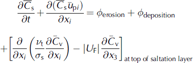
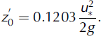
The NEMO numerical model is based on a physical model for saltation and turbulent diffusion (Reference Naaim, Naaim-Bouvet and MartinezNaaim and others, 1998), ignoring sublimation, which is less important at the avalanche-release area scale (Fig. 1). The saltation layer is described by its height, concentration and two turbulent friction velocities, one for the solid phase and one for the gaseous phase. The top of the saltation layer is considered as the lower boundary condition for the suspension layer. The suspension layer is described by mass and momentum conservation equations. These equations were formulated both for the solid phase and the gaseous phase. The interaction between these two phases was taken into account by an equation based on the drag force of a particle in a turbulent flow. Turbulence was modeled by the k–ε model, where a turbulence reduction with increasing concentration was introduced. The exchange between the saltation layer and the snow cover was described by an erosion and deposition model. The mesh was adapted to the temporal change of the drift.
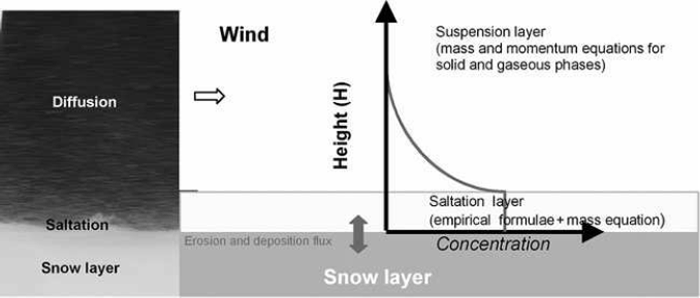
Fig. 1. Characteristics of the numerical model.
This model can briefly be described by the separate flow equations for each layer (saltation, suspension and snow cover); additional information can be found in Reference Naaim, Naaim-Bouvet and MartinezNaaim and others (1998).
In the suspension layer
Air mass conservation:
Particle mass conservation:
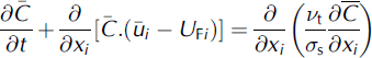
Momentum conservation:
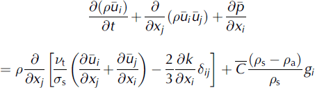
with ![]() . A k–ε model modified by the presence of particles is used to close the system.
. A k–ε model modified by the presence of particles is used to close the system.
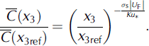
The solutions of the equations in a case of boundary layer over flat area for steady-state drifting snow lead to the blowing-snow mass density for a given particle radius:
In the saltation layer
Particle mass conservation:

where ρ
a
is air density (kg m−3), ρ
s
is blowing-snow particles density (kgm−3), ![]() is the mean air velocity component in the Oxi direction (ms−1) in the suspension layer,
is the mean air velocity component in the Oxi direction (ms−1) in the suspension layer, ![]() is the mean particle velocity component in the Oxi direction (m s−1) in the saltation layer, u
* is the friction velocity (m s−1), u
*t is the threshold friction velocity (ms−1), x
3 is the vertical component,
is the mean particle velocity component in the Oxi direction (m s−1) in the saltation layer, u
* is the friction velocity (m s−1), u
*t is the threshold friction velocity (ms−1), x
3 is the vertical component, ![]() is the mean particle concentration in the suspension layer (kgm−3),
is the mean particle concentration in the suspension layer (kgm−3), ![]() is particle concentration in the saltation layer (kgm−3),
is particle concentration in the saltation layer (kgm−3), ![]() is the maximum particle concentration in the saltation layer (kgm−3), νt is the turbulent viscosity coefficient (m2s−1),
is the maximum particle concentration in the saltation layer (kgm−3), νt is the turbulent viscosity coefficient (m2s−1), ![]() is the mean pressure (N m−2), g is gravitational acceleration (ms−2), σ
s is the Schmidt number, Kis the von Karman constant and k is the turbulent kinetic energy (m2 s−2).
is the mean pressure (N m−2), g is gravitational acceleration (ms−2), σ
s is the Schmidt number, Kis the von Karman constant and k is the turbulent kinetic energy (m2 s−2).
2.2. Input parameters
The model needs a set of input parameters including fall velocity, threshold shear velocity, shear velocity, mass concentration and roughness. NEMO has been tested by comparing leeward and windward drift equilibrium obtained in a wind tunnel near a small-scale snow fence (Reference Naaim, Naaim-Bouvet and MartinezNaaim and others, 1998) with all these input parameters known; moreover these parameters remained constant throughout the experiment. However, the computation results were often less conclusive when compared to the results of field experiments (Reference Michaux, Naaim-Bouvet and NaaimMichaux and others, 2001) conducted at Col du Lac Blanc. It is true that the fully coupled wind and snowdrift model was not used in this case because of the time required for calculation, and that additional assumptions were made. However, it is probable that the most important source of uncertainty stems from the lack of accurate evaluations of the input parameters needed for the numerical model. In fact, at our experimental site, where NEMO was tested (Reference Michaux, Naaim-Bouvet and NaaimMichaux and others, 2001), only wind speed and direction as well as a snowdrift sensor based on an acoustic principle could be accessed. This snowdrift sensor provided information on whether or not snowdrift events had occurred.
Thus, some parameters were estimated from semi-empirical relationships obtained with data probably collected under different conditions than those encountered in the Alps in terms of topography and snow types. Therefore, the following relationships from Pomeroy and Gray’s (Reference Pomeroy and Gray1990, Reference Pomeroy and Gray1993) work were used:

Q s is the total mass-transport rate per unit of lateral dimension in the saltation layer (kgm−1 s−1), hs is the height of the saltation layer (m), C salt is the maximum drift density of saltating snow (kgm−3) and z 0 is the aerodynamic roughness (m).
In our case, the value of σ s U F was estimated based on the experimental dataset published by Reference Mellor and FellersMellor and Fellers (1986), which consisted of 1200 usable data from Reference Mellor and RadokMellor and Radok (1960) and Reference Budd, Dingle, Radok and RubinBudd and others (1966) obtained by anemometers and aerodynamic snow collectors mounted in pairs on vertical masts in Antarctica. Velocity and concentration profiles were used to calculate the exponent of Equation (4) (Reference Naaim-Bouvet, Naaim and MartinezNaaim-Bouvet and others, 1996; Fig. 2):
The increase of σ s U F with u* is caused by the increase of the mean diameter of the wind-borne particles with increasing u*.

Fig. 2. Change in product σsUF as a function of u* (Reference Naaim-Bouvet, Naaim and MartinezNaaim-Bouvet and others, 1996).
Despite the approximations above, accurate evaluation of the input parameters needed for the numerical model remains an open question. Few quantitative measurements from Alpine sites are available (Reference Doorschot, Lehning and VrouweDoorschot and others, 2004), which is why, in the last few years, we returned to the field to improve measurements of drifting snow at Col du Lac Blanc pass by testing these empirical formulae in an alpine context.
3. In Situ Measurements of Drifting Snow
3.1. Description of the site and the available instrumentation
The experimental site (Reference Naaim-Bouvet, Durand, Michaux, Guyomarc’h, Naaim and MerindolNaaim-Bouvet and others, 2000) is located at the Alpe d’Huez ski resort near Grenoble, France. The large north-south-oriented pass (Col du Lac Blanc) has been dedicated to the study of blowing snow in high mountainous regions for approximately 20 years. The area consists of relatively flat terrain on a length of about 300 m. The slope then becomes steeper both in the northern and southern parts. Far away, the terrain becomes flat again and lakes occupy many depressions. In the eastern part of the site stands a high alpine range, ‘Grandes Rousses’, culminating at about 3500m a.s.l. with Pic Bayle, whereas a lower summit (Dome des Petites Rousses) lies on the west. The pass orientation and the specific configuration of the ‘Grandes Rousses’ range make the pass very close to a natural wind tunnel. North or south account for 80% of the wind directions.
In 2000, when the NEMO model was first validated at Col du Lac Blanc (Reference Michaux, Naaim-Bouvet and NaaimMichaux and others, 2001), several parameters (air temperature, wind direction and speed, snow depth, water equivalent of precipitation) were recorded every 15 min. This standard measurement device was supplemented by six acoustic snowdrift sensors, consisting of a miniature microphone located at the base of a 2 m long aluminium pole and initially designed at Cemagref and manufactured by AUTEG (Reference Font, Naaim-Bouvet and RousselFont and others, 1998; Reference Michaux, Naaim-Bouvet and NaaimMichaux and others, 2001). The pole was exposed to the snow particle flux, and part of the flux impacted on the pole during blowing snow. The sound produced by these impacts is recorded as an electrical signal. The sensors were not calibrated, but reliably recorded the beginning and end of blowing-snow events. The three-dimensional spatial distribution was investigated using a network of metallic snow poles on erosion zones as well as on accumulation zones. The instrumentation was then progressively improved and updated.
3.1.1. Wind measurements
In 2004, the site was fitted with an ultrasonic anemometer (Metek USA-1) set up at 3.3 m height. The sonic anemometer can simultaneously record each component of the wind vector at time rates up to 10Hz. Moreover, temperature estimation is computed from a measure of the sound celerity at the same time rate. In 2007, six cup anemometers (A1–A6) were mounted on a 10 m vertical mast with logarithmically vertical spacing (Fig. 3). Temperatures (T1 and T2) were monitored by platinum resistance thermometers at the same place as A3 and A6, and the experimental set-up was completed by a snow depth sensor (H1). The mast aims at better investigation of the friction velocity and the aerodynamic roughness.
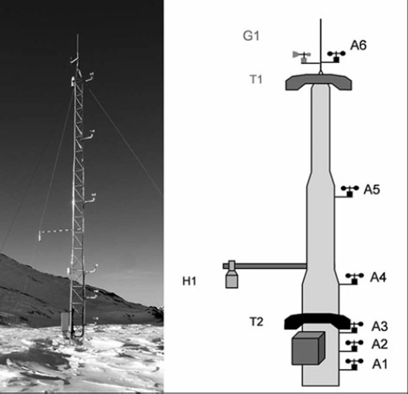
Fig. 3. A 10m tower with six anemometers including snow-depth and temperature measurements.
3.1.2. Blowing-snow measurements
If sensors for wind measurements are reliable and accurate, this is still not the case for all blowing-snow sensors. Different techniques are available such as acoustic (Reference Chritin, Bolognesi and GublerChritin and others, 1999; Reference Michaux, Naaim-Bouvet and NaaimMichaux and others, 2001), optical (Reference Sato, Kimura, Ishimaru and MaruyamaSato and Kimura, 1993) and pulse-counting techniques (Reference Bintanja, Lilienthal and TügBintanja and others, 2001). Extensive and time-consuming tests are sometimes still needed before interpreting the results quantitatively.
FlowCapt acoustic sensor. FlowCapt consists of Teflon-coated tubes fitted with electroacoustic transducers (Fig. 4). During snowdrift events, particles impact the tubes, inducing acoustical pressure inside the tubes. This is picked up by the transducers. The signal is then filtered and amplified. The device is delivered with complete calibration, which is performed using the controlled flux of PVC particles (Reference Chritin, Bolognesi and GublerChritin and others, 1999). The sensor gives an estimation of the mass flux of snow (g m−2 s−1). The signal intensity and the momentum of snow grains are assumed to be related by a physical law, which is supported by laboratory experiments performed with PVC balls (Reference Chritin, Bolognesi and GublerChritin and others, 1999). The estimated flux is computed using
where Fd denotes the flux data displayed by the sensor, and Signal the electrical voltage picked up by the data logger (mV). The FlowCapt set-up at Col du Lac Blanc provided profiles of snow fluxes 0–180cm above ground level.
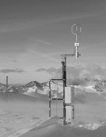
Fig. 4. FlowCapt with six vertical tubes in 2004.
It is thus possible to obtain an estimation of the transport rate with respect to the height above the snow surface. The use of concurrent wind-profile data made it possible to evaluate drift density data and therefore the product of settling velocity times Schmidt number.
For theoretical reasons, which are explained below, the six tubes were set up horizontally in 2008 (Fig. 5).
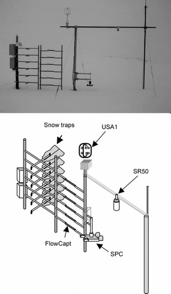
Fig. 5. Final configuration of the snowdrift sensors test bed at Col du Lac Blanc in 2008.
Snow Particle Counter. Since 2008 the drifting-snow flux has also been measured with the Snow Particle Counter (SPC-S7, Niigata Electric), which works on an optical method (Reference Sato, Kimura, Ishimaru and MaruyamaSato and Kimura, 1993). The diameter and the number of blowing-snow particles are detected by their shadows on photosensitive semiconductors. Electric pulse signals of snow particles passing through a sampling area are sent to an analysing logger. The SPC thereby detects particles 50–500 μm in size, divides them into 32 classes and records the number of particles every 1 s. Assuming spherical snow particles, the horizontal snow mass flux q is calculated as (Reference Sugiura, Nishimura, Maeno and KimuraSugiura and others, 1998)
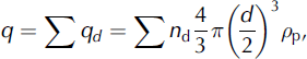
where qd (kg m−2 s−1 is the horizontal snow mass flux for the diameter d (m), nd is the number flux of the drifting-snow particles and ρ p is the density of the drifting-snow particles (917kgm−3). It must be pointed out that the flux value is given for a small sampling area (50 mm2).
Butterfly net. Specific field measurements have been performed to obtain an estimation of snowdrift from mechanical snow traps that could be compared with data recorded by FlowCapt and SPC (Fig. 6). The traps consisted of ‘butterfly nets’, i.e. a metallic frame with a nylon bag attached. The mixture of air and snow grains goes through the traps and, while the snow is collected in the bag, the air escapes through the pore. The cross-section is similar to that of FlowCapt, i.e. 0.007776 m2. Such snow collectors disturb the flow, and their efficiency depends on the aerodynamic design. Nonetheless, they are still the best reference and less expensive than SPC sensors, though they require the presence of experimenters under cold and windy conditions.
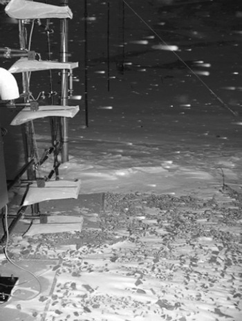
Fig. 6. Mechanical snow traps.
Field tests and intercomparison. Intercomparison tests with FlowCapt, SPC and snow-net collectors have already been done in the past. Reference Font, Sato, Kosugi, Sato and VilaplanaFont and others (2001) used the SPC to calibrate four different mechanical traps in a cold wind tunnel (Cryospheric Environment Simulator, Japan) with disintegrated snow. They showed that the net-type traps underestimate transport in low-transport conditions, but as transport increases, the difference tends to zero. Reference LehningLehning and others (2002) presented the first evaluation of the accuracy of an acoustic sensor by comparing snow traps and acoustic sensors both in a cold wind tunnel (Jules Verne wind tunnel, France) and under natural conditions in the Alps. The results were disappointing: they confirmed preliminary results that acoustic sensors are only suitable for giving qualitative or semi-quantitative results, as there are still some calibration issues to resolve. Reference Savelyev, Gordon, Hanesiak, Papakyriakou and TaylorSavelyev and others (2006) deployed snow bags and a FlowCapt device and other instruments related to drifting-snow monitoring in Franklin Bay, Canada. They showed that FlowCapt overestimates snow mass flux as determined by snow bags by an order of magnitude. This is why we continue calibration at Col du Lac Blanc (Reference Cierco, Naaim-Bouvet and BellotCierco and others, 2007). During some snowdrift events, each segment of FlowCapt was compared to mechanical snow traps whose cross-sections were designed to be exactly the same as the FlowCapt cross-sections.
The shear velocity, u *, was estimated from one measurement point (ultrasonic anemometer 3.3 m high) assuming a logarithmic profile in the atmospheric boundary layer and Pomeroy’s formula for z 0 (Equation (11)). In Figure 7, segment 1 is near the ground (0.3 m) and segment 3 is the highest (0.9 m) on which significant blowing snow is recorded. The correlation between FlowCapt and the snow bag is significant for a given segment (Fig. 7) and consequently for a given height. However, the behaviour of the sensor depends on the height: the higher FlowCapt is, the greater is the slope of the linear regression line (4.9 for 0.15 m, 15.07 for 0.45 m and 27.2 for 0.75 m).
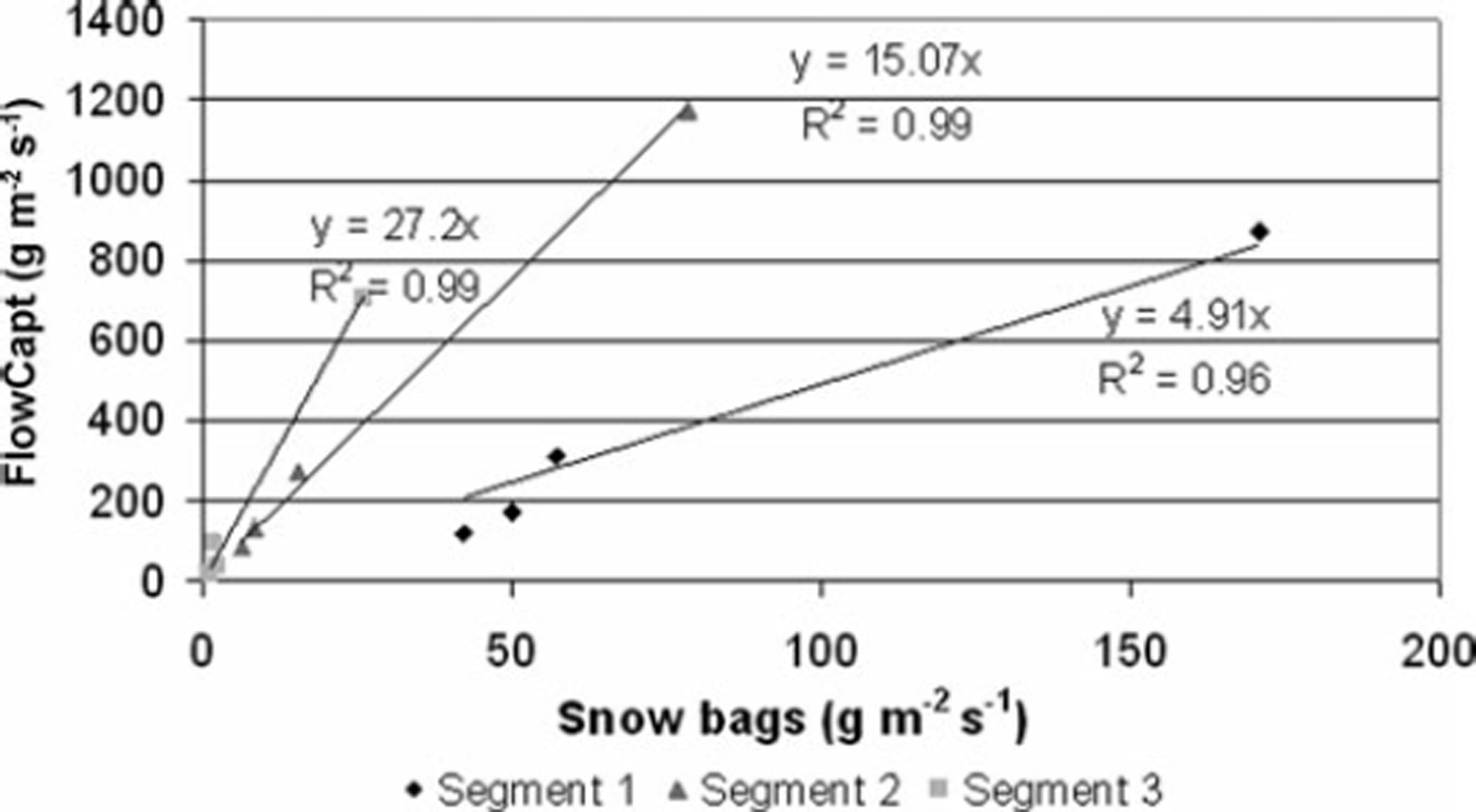
Fig. 7. Relation between the snow flux recorded on FlowCapt and measured by the mean of snow bags for different heights.
As the main difference for different heights was the particle horizontal velocity which is considered equal to the wind speed at the same height, all the data were re-treated considering this new parameter (Reference Cierco, Naaim-Bouvet and BellotCierco and others, 2007). In this way, it was established that the poor treatment of particle velocity, which is not taken into account in the initial calibration curve, results in aberrations in the recorded data.
A correction algorithm based on statistical calibration of the sensor for rounded grains was proposed. The new calibration curve is
with B= 1.49 for rounded grains.
It should be noted that Fd varies with the inverse of the particle velocity to the fourth power, so that the acoustic sensor appears to be insufficiently accurate whatever the calibration may be (the value of B depends on the particle type). In order to improve the calibration and as the velocity gradient is high near the ground, we set up the six tubes horizontally in 2008 (Fig. 5).
During winter 2008/09, the only year during which the SPC and FlowCapt were set up side by side, ten drifting-snow events were identified. For all the events (except when the SPC is buried under the snow cover), FlowCapt and the SPC give similar values for the occurrence of drifting snow (Fig. 8), but FlowCapt systematically overestimates snow mass flux as determined by snow bags (Fig. 10).
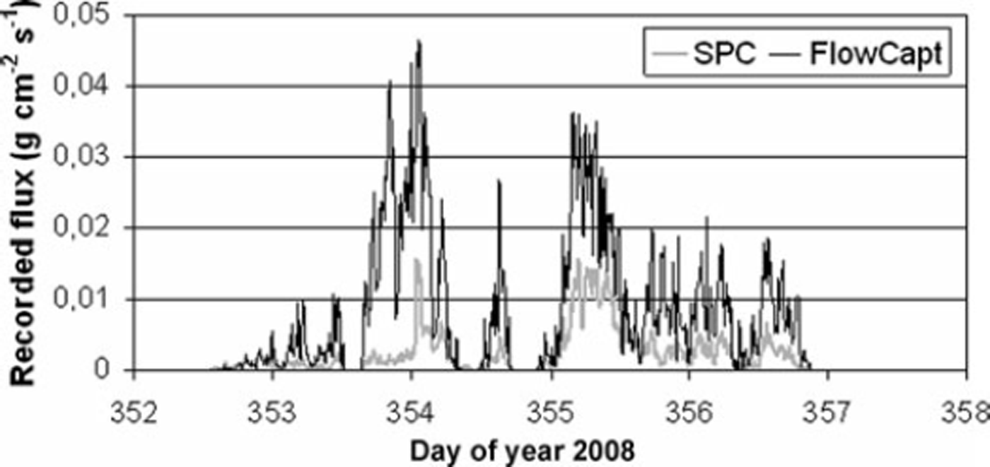
Fig. 8. Data from a prolonged drifting snow (17–22 December 2008): comparison between SPC and FlowCapt.
The particle size distribution cannot be measured at a given height since the snow depth changes, but event 5 is a representative sample of the encountered blowing-snow events during winter 2008/09. Generally the mode, which is the peak-frequency diameter, is centred around 80 μm (Fig. 9a), but when we consider the frequency volume distribution, the peak-frequency diameter is centred around 200 μm (Fig. 9b). The minimum diameter class seems to be underestimated, as there is no physical explanation for all particles having a diameter greater than 50 μm during blowing snow; furthermore, particles with a diameter <50μm were observed during blowing-snow events (Reference Gordon and TaylorGordon and Taylor, 2009). However, the weight of such particles in the calculation of the horizontal snow mass flux is negligible. The maximum diameter class (493 μm) includes all the larger particles, but, in this case, the weight of such particles in the calculation of the horizontal snow mass flux is important, and some underestimation of snow flux could appear. As noticed by Reference Sugiura, Nishimura, Maeno and KimuraSugiura and others (1998), the frequency distribution becomes flatter with increasing wind (Fig. 9a, event 7) due to the increase in wind-borne particle diameter with u*. Conversely, the frequency of smaller particles increased with decreasing wind (Fig. 9a, event 4). We also propose that the particle diameter is calculated from a projected area difference from an equivalent diameter based on volume for non-spherical diameter. Reference Sato, Kimura, Ishimaru and MaruyamaSato and Kimura (1993) have estimated this error theoretically for spheroid and square-pillar shapes. Nevertheless the SPC has been used extensively and is recognized to give accurate results. During winter 2008/09, we compared snow mass flux recorded by the SPC and FlowCapt and deduced from snow bags (Fig. 9b). It was shown that, for the given event (rounded grains), the SPC and snow bags show good agreement. We first compare snow mass flux recorded by the SPC and FlowCapt and then use the new calibration curve previously proposed (Equation (15)). The wind speed at the height of the FlowCapt tube is estimated from the 10 m tower with six anemometers. It can be seen that the new calibration affects the snow flux estimation (Fig. 11a and b); the slope of the linear regression line increases but is still very different from 1, and data are more scattered, with a decreasing correlation coefficient (R 2 = 0.26).
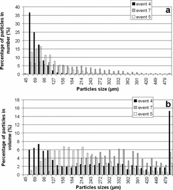
Fig. 9. Frequency distribution of drifting-snow particle diameter (a) and frequency volume distribution of drifting-snow particle diameter (b) (event 4: V 8.4m= 5.8ms−1, H SPC = 0.2m, duration 940min; event 5: V 8.3m =10ms−1, H SPC = 0.45m, duration 1750 min; event 7: V 8.6m =13ms−1, H SPC = 0.28m, duration 700 min).
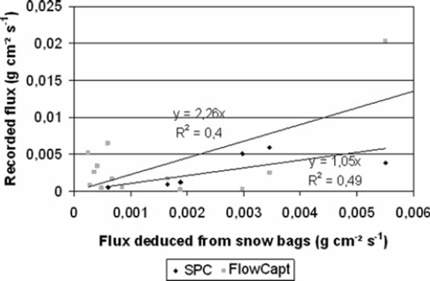
Fig. 10. Comparison between snow mass flux recorded by SPC and FlowCapt and deduced from snow bags.
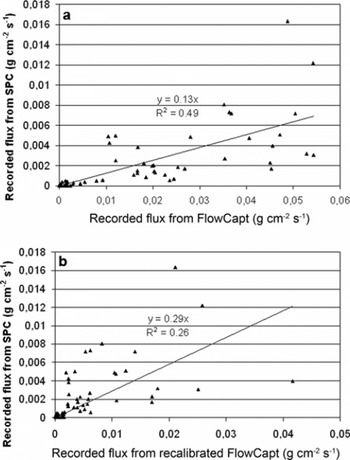
Fig. 11. Comparison between snow mass flux recorded by SPC and FlowCapt (a) and by SPC and recalibrated FlowCapt (b).
3.2. Results
3.2.1. Determination of aerodynamics roughness
The friction velocity is determined by a profile method using data from the 10m tower with six anemometers. Generally, the near-surface distribution with height of time-averaged wind speed varies logarithmically.
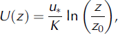
with U the wind speed (m s−1), z (m) the height above the snow cover, K the von Kármán constant (usually taken to be 0.4) and z0 the surface roughness (m), which is independent of the wind speed.
Thus, in a semi-log space, the friction velocity u* is proportional to the inverse of the slope of the straight line, and the aerodynamic roughness z0 represents the intercept. The logarithmic profile is valid only in neutral conditions and for flat terrain. Due to the surrounding topography at Col du Lac Blanc, some deviation from this profile could occur. First we have tested that it is still approximately valid close to the surface at the measurement point. Generally, the eddy correlation method can also be applied using the ultrasonic anemometer, but this was not done since some problems occurred with the ultrasonic anemometer during the period of interest. However, comparison of the two methods (profile method and eddy correlation method) is at hand for other measurements at Col du Lac Blanc.
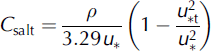
Snow transport alters the effective roughness of the bed by extracting momentum from the wind due to the necessary horizontal acceleration of drifting-snow particles. The resulting roughness measured by extrapolating the velocity profile outside the saltation layer shows a dependence on friction velocity. The wind modification during saltation is perceived by the flow as an increase in surface roughness due to the straight line extrapolations of the wind velocity on a log-linear plot from above the saltation layer to u = 0 (Reference Anderson, Haff, Barndorff-Nielsen and WillettsAnderson and Haff, 1991; see Fig. 15). According to Reference OwenOwen (1964), the saltation layer acts like a solid roughness on the flow and leads to a roughness height proportional to the square of the friction velocity (Equation (11)). Reference Pomeroy and GrayPomeroy and Gray (1990) proposed a value of 0.1203 for C 0 for land-based snow cover. This is nearly an order of magnitude greater than Reference TablerTabler’s (1980) (C 0 = 0.02648) and Schmidt’s (1990) values for lake ice-based snow covers.
Reference Andreas, Jordan, Guest, Persson, Grachev and FairallAndreas and others (2004) develop a new parameterization for z 0 as function of the friction velocity over snow.
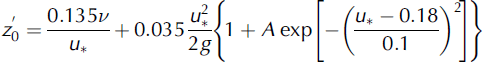
In this case, ![]() models the aerodynamic smooth regime,
models the aerodynamic smooth regime, ![]() models the saltation regime and the last term reflects the roughness of the surface as A depends on the tested site.
models the saltation regime and the last term reflects the roughness of the surface as A depends on the tested site.
The present study explores how the measured z0 correlates with values of u* during a drifting-snow event at Col du Lac Blanc. There is a limited number of velocity data periods that occur during thermally neutral periods. In the following, results where R 2<0.9 and potential temperature difference is >1 were rejected.
The following observations can be made:
For the same value of friction velocity, roughness values are dispersed, leading to a low coefficient of determination.
Without drifting snow, the surface roughness could depend on the wind direction, because the topography of the two fetches is different (Fig. 12a).
The proportionality of z′ 0 to the square of the friction velocity seems to be confirmed, but once again the coefficient of determination is rather low.
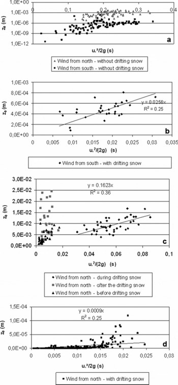
Fig. 12. Roughness height plotted against friction velocity.
Given the formation of aeolian features (e.g. sastrugi), the roughness height could be greater after the storm (Fig. 12c). The change in the surface roughness during the snowstorm could perhaps explain the rather low coefficient of determination. There are also probably some topographic effects due to up- and downwind slopes. The value of C 0 depends on the snowdrift events (Fig. 12b–d) for the same site. There is a two orders of magnitude difference between the different values. Except for the smallest value (Fig. 12d), the range corresponds to values observed by Reference TablerTabler (1980), Reference Pomeroy and GrayPomeroy and Gray (1990) and Reference Andreas, Jordan, Guest, Persson, Grachev and FairallAndreas and others (2004).
As the apparent increase of roughness is related to the exchange of momentum between wind and snow particles in the saltation layer, the wide variation of C 0 is not surprising: the roughness must be related to the snow flux in the saltation layer, so the threshold friction velocity must also be taken into account (Equation (11)).
For an accurate estimation of the input parameters for NEMO, a semi-empirical model is not sufficient because the coefficient C0 depends on the drifting-snow event and varies by at least a factor of 1–100. It is important to note that an error in estimating z0 leads to an error in estimating u* when using only one wind measurement point.
3.2.2. Determination of σsUF
In steady state, the transport of snow particles is governed by a balance between gravitational settling and turbulent diffusion leading to Equation (4) for the concentration profile. The implicit assumption is that the particle size distribution does not change significantly with height. Velocity and concentration profiles can be used to calculate the exponent of the equation. As a first step, all data from the 2004/05 winter season for blowing-snow events involving rounded grains had to be reprocessed using the new calibration curve (Equation (15)). Such events have been isolated using Crocus (Reference Brun, David, Sudul and BrunotBrun and others, 1992), which simulated the different physical and mass processes into the snow cover and its complete stratigraphy. The value of u* is calculated from a single wind measurement point at 3.3 m, using the semi-empirical formulae for z0 with C0 = 0.1203. This leads to the curve relating σsUF and u* (Fig. 13)
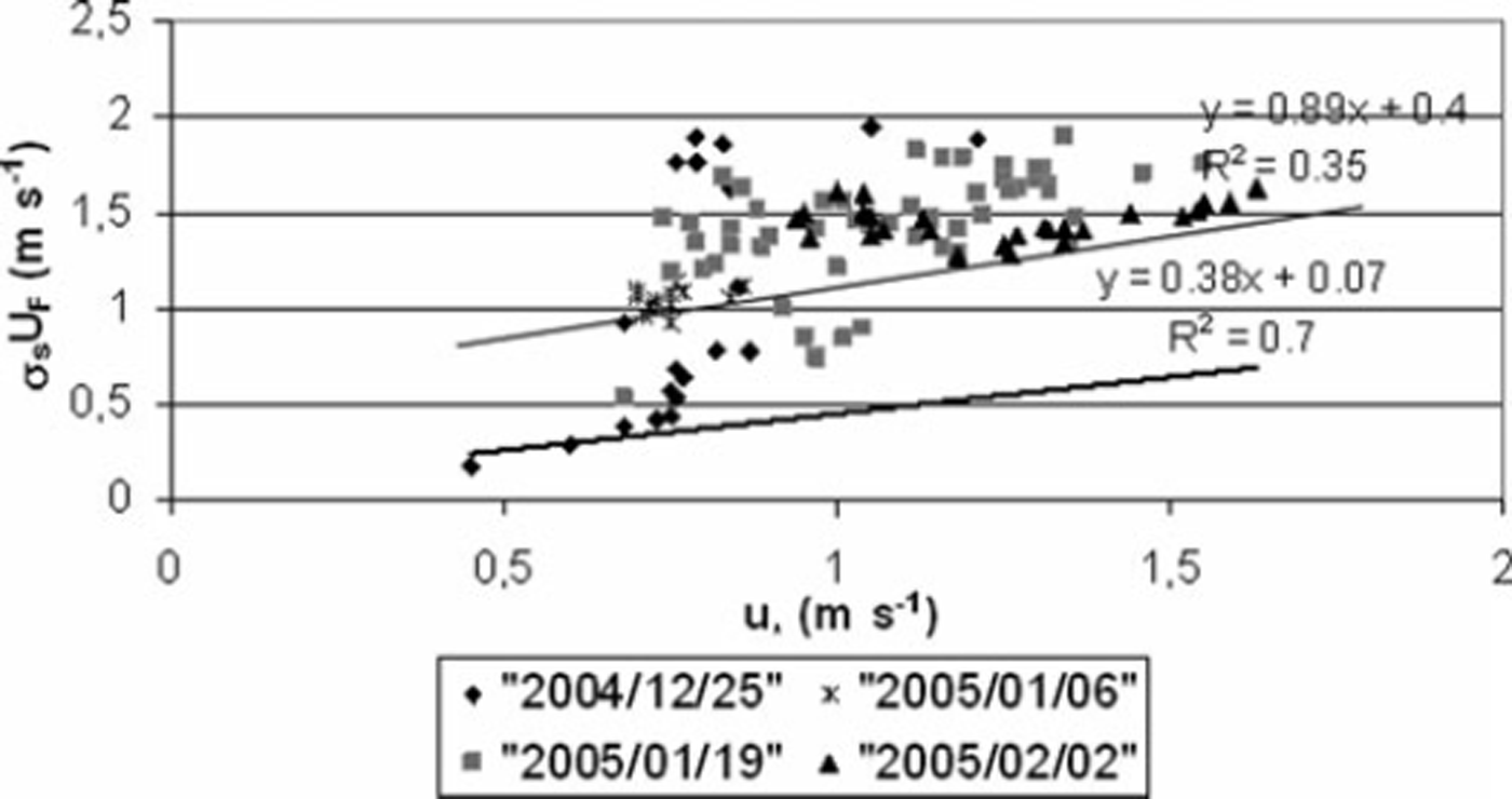
Fig. 13. Change in product σsUF as a function of u* at Col du Lac Blanc from FlowCapt and one wind measurement point (gray line represents relationship obtained with data from Antarctica). Dates: year/month/day.
It could be concluded from Figure 13 that the use of the empirical formula obtained from Antarctic data seems to underestimate σsUF in the French Alps. But in fact it was seen in section 3.1.2 that FlowCapt was not deemed suitable for research applications and that an error in estimating z0 leads to an error in estimating u* when using only one wind measurement point. This is why we returned to the traditional robust mechanical traps coupled with the 10m mast to determine u* and z 0. Of course, it would be better to use several SPCs as done by Reference Mann, Anderson and MobbsMann and others (2000) or Reference Gordon and TaylorGordon and Taylor (2009), but only one sensor was available on our experimental site.
Contrary to what we concluded previously from FlowCapt data processing, the relation between σsUF and u* slightly differs from those obtained in Antarctica: the regression obtained in Antarctica still lies in the scatter of the data. If the value of u* is calculated from a single wind measurement point at 8.8m, using the semi-empirical formulae for z0 with C0 = 0.1203, points are shifted to the right in Figure 14, but the slope of the regression line does not differ significantly. The empirical formula obtained from Antarctic data for σsUF can be used at Col du Lac Blanc. Nevertheless, mechanical measurements for higher friction velocity must be conducted to confirm this trend.
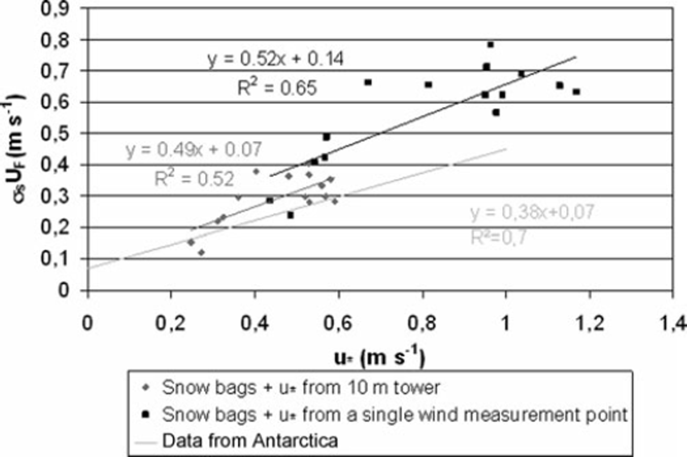
Fig. 14. Change in product σ s U F as a function of u* at Col du Lac Blanc (snow-bag measurements taken in March 2008: 75 data available; rounded grains).
It is also interesting to compare the data processing we did in 1996, with the 1200 usable data from Reference Mellor and RadokMellor and Radok (1960) and Reference Budd, Dingle, Radok and RubinBudd and others (1966) obtained in Antarctica, with more recent experimental data obtained by Reference Mann, Anderson and MobbsMann and others (2000) or Reference Gordon and TaylorGordon and Taylor (2009). Reference Mann, Anderson and MobbsMann and others (2000) measured concentration profiles using six particle counters at the Halley research base in Antarctica; they found that the settling velocity (assuming that the Schmidt number is equal to 1) increases with friction velocity σs U F = 0.4u* up to u* = 0.375 ms−1, after which it is approximately constant. With two similar particle counters, Reference Gordon and TaylorGordon and Taylor (2009) showed a slightly higher settling velocity, with a continuous increase with friction velocity (even for u*>0.375 ms−1), at Franklin Bay, Canada. These are very similar to our own results. As pointed out by Reference Gordon and TaylorGordon and Taylor (2009), the continuous increases of σsUF with u* indicate that larger particles were available in experiments done by Reference Mellor and RadokMellor and Radok (1960), Reference Budd, Dingle, Radok and RubinBudd and others (1966) and Reference Gordon and TaylorGordon and Taylor (2009). However, some authors consider that the Schmidt number is lower than 1. Reference Naaim and MartinezNaaim and Martinez (1995) obtained a value of 0.5 in a wind tunnel for PVC particles. Listen and others (1994) used a value of 0.5 in a computational blowing-snow model referring to Reynolds’ work (1976) for planar flows. The same orders of magnitude are found by Sanjeev and Bombardelli (2009) when they assess diverse turbulence closure in the simulation of dilute sediment-laden open-channel flows.
3.2.3. Determination of the drifting-snow concentration profile
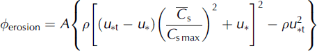
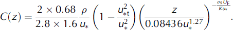
Combining results from measurements on a snow-covered plain and theory, Reference Pomeroy and GrayPomeroy and Gray (1993) proposed Equation (10) for determining C salt, the mean drift density of saltating snow (kgm−3). C salt is also the lower boundary condition of Equation (5) for the suspension model. Following Pomeroy and Gray, the height h* that delineates the saltation and suspension layers can be approximated by
This value was found by extrapolating the modelled suspension mass concentration towards the saltation layer until they approximate the mean drift density C salt. For u*< 1.05 m s−1, this leads to suspension drift density greater than those calculated with the lower boundary condition equal to the height of the saltation layer (Equation (9)). Equation (4) becomes
Using Equation (19), snowdrift events from 4–5 March 2008 and 27 February 2009 have been simulated. In both cases, the value of σsUF used comes from the linear regression of the data obtained with snow traps (Fig. 14) and u* was determined from a profile method thanks to the 10 m tower with six anemometers. Data for height <10 cm were rejected because near the saltation layer (in the so-called modified saltation layer) particles are in transition from saltation to suspension and probably have not achieved full horizontal wind velocity.
It can be seen from Figures 15–17 that the semi-empirical formulation proposed by Reference Pomeroy and GrayPomeroy and Gray (1993) overestimates the profile by one order of magnitude. Our comments on this are:
-
1. Results concerning aerodynamic roughness and concentration are in agreement: as the apparent increase of roughness is related to the exchange of momentum between wind and snow particles in the saltation layer, less snow flux leads to a smaller aerodynamic roughness.
-
2. Works of Pomeroy and Gray’s have been established for a steady state and a fully developed flow, which could imply a fetch with a constant friction velocity and snow supply from 150 to 300 m for the lowest 0.3 m of the atmospheric boundary layer for a snowdrift event (Reference TakeuchiTakeuchi, 1980). Such conditions are rarely or never encountered in an Alpine context. Therefore the simulated concentration must be considered a maximum value. This was precisely the idea we developed in the numerical model NEMO, in which the inertia of snow erosion and deposition is taken into account by means of erosion and deposition flux: Cs alt (Equation (10)) is considered as the maximum snow concentration in the saltation layer (Reference Naaim, Naaim-Bouvet and MartinezNaaim and others, 1998). Logically, input concentration profiles of such a model must also take into account inertia of snow erosion and deposition upwind of the zone of interest. The simulated profile (Equation (19)) cannot apply as a concentration profile boundary condition: the measured concentration profile must be the upwind boundary condition, or at least a long fetch distance must be simulated upwind of the zone of interest.
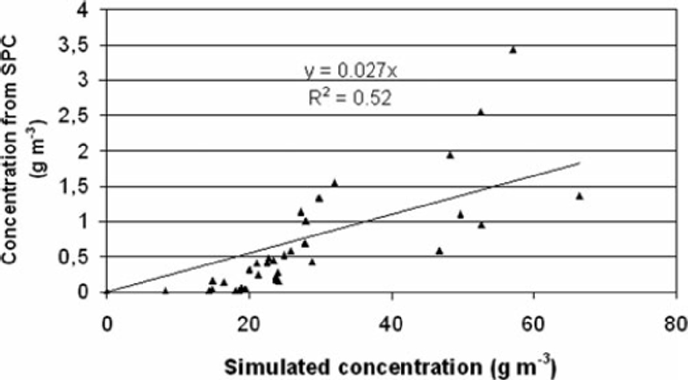
Fig. 15. Snowdrift concentration obtained by SPC on 27 February 2009 as function of simulated concentration obtained using Pomeroy and Gray’s semi-empirical formulae for saltation layer coupled with theoretical approach for the diffusion layer (Equation (19)).
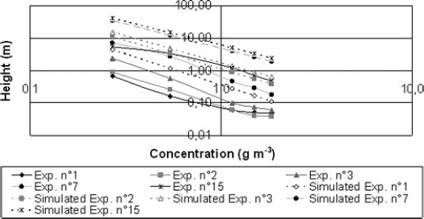
Fig. 16. Snowdrift concentration profiles obtained by snow traps (solid lines) on 4 March 2008 and by Pomeroy’s semi-empirical formulae for saltation layer coupled with theoretical approach for the diffusion layer (dotted lines) (Equation (19)).
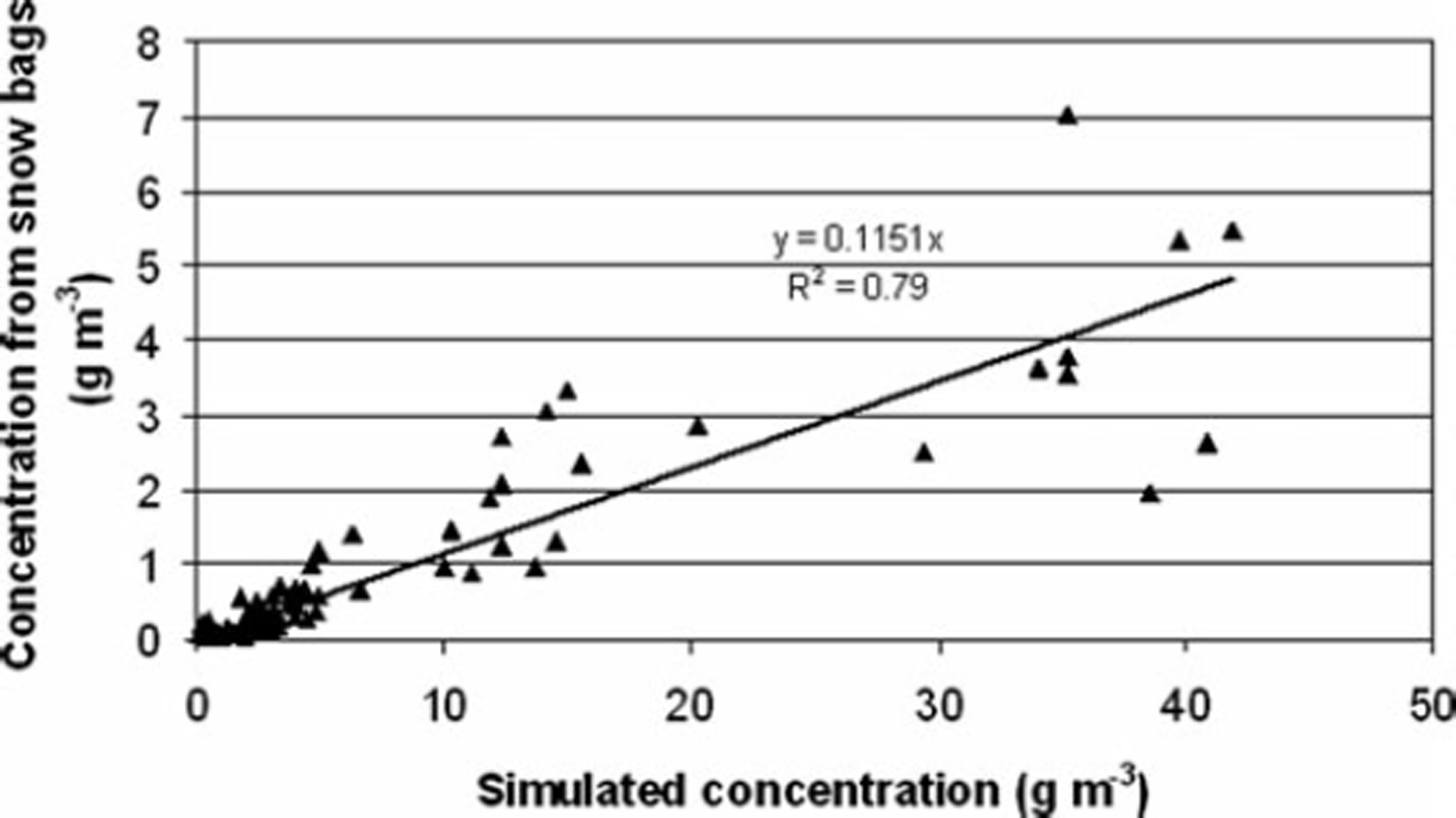
Fig. 17. Snowdrift concentration obtained by snow traps on 4 March 2008 as function of simulated concentration obtained using Pomeroy and Gray‘s semi-empirical formulae for saltation layer coupled with theoretical approach for the diffusion layer (Equation (19)).
4. Conclusion and Further Developments
Accurate input parameters cannot be omitted when studying the ability of a numerical model to reproduce field experiments. In the case of NEMO, the use of empirical formulae is not enough and their validity has been tested by improving instrumentation dedicated to blowing-snow setup at Col du Lac Blanc.
It was shown for the studied drifting-snow events that (1) the square of the friction velocity seems to be confirmed, but with a varying constant depending on the snowdrift event and a poor coefficient of determination; (2) values of σ s UF are relatively well approximated by empirical formulae obtained from Antarctica data; and (3) snowdrift concentration profiles obtained by Pomeroy’s semi-empirical formulae for the saltation layer coupled with a theoretical approach for the diffusion layer lead to an overestimation of the concentration profiles.
However, few accurate concentration profiles have been obtained because such data require the presence of an experimenter; at the present time, data from FlowCapt are not sufficiently accurate for research purposes. The setting-up of a second SPC in the near future will allow us to increase the dataset and perhaps better investigate the relation between aerodynamic roughness and snow flux and also the relation between the friction velocity and σ s UF. The Schmidt number is a key factor for predicting sediment transport in suspension. Thus the next step will be to combine concentration profiles using particle counters and direct determination of particle vertical velocity by a camera system (as used by Reference Gordon and TaylorGordon and Taylor, 2009) to better investigate the value of the Schmidt number.
Acknowledgements
We thank F.-X. Cierco, F. Perault, F. Ousset, X. Ravanat and R. Beguin for support with the field measurements.


