2.1. Vorticity

The vorticity is a well-known quantity in turbulence. Its magnitude will be mostly used here as

(2.1)\begin{equation} \omega=\| \boldsymbol{\nabla} \times \boldsymbol{u}\|. \end{equation}

2.2. Increments and structure functions

The traditional basic tool to study intermittency is via scaling of the velocity structure functions of order $p$, defined as

(2.2)\begin{equation} S_p(\ell)={\left\langle \left(\delta_{\boldsymbol{\ell}} u\right)^p\right\rangle}_{\|\boldsymbol{\ell}\|=\ell}. \end{equation}

Here, $\delta _{\boldsymbol {\ell }} u$ is the longitudinal velocity increment at scale $\ell$, defined as

(2.3)\begin{equation} \delta_{\boldsymbol{\ell}} u ={\hat{\boldsymbol{\ell}}} \boldsymbol{\cdot} \left(\boldsymbol{u}(\boldsymbol{x}+{\boldsymbol{\ell}})-\boldsymbol{u}(\boldsymbol{x})\right), \end{equation}

where $\hat {\boldsymbol {\ell }}$ is the increment direction. Throughout the paper, the notation $h$ refers to the local Hölder regularity of $\delta _{\ell } u$ so that $\delta _{\ell } u \sim \ell ^h$. Muzy, Bacry & Arneodo (Reference Muzy, Bacry and Arneodo1991) argued that wavelet-based velocity increments $\delta W_{\ell }$ may provide more robust results, via the so-called wavelet transform modulus maxima method. The use of wavelets (Farge Reference Farge1992; Schneider & Vasilyev Reference Schneider and Vasilyev2010) allows us to separate strong vorticity structures from the noise. We use a wavelet such that the first moment vanishes. This allows us to explore Hölder exponents lower than one. The velocity increments are defined via the wavelet transform of the tensor $\partial _j u_i$

(2.4)\begin{equation} G_{i,j}(\boldsymbol{x},\ell)=\int {\boldsymbol{\nabla}_{j} \phi_{\ell}(\boldsymbol{r}) u_i(\boldsymbol{x}+\boldsymbol{r})\,\mathrm{d}\boldsymbol{r}}, \end{equation}

where $\phi _{\ell }(x)=\ell ^{-3}\phi (x/\ell )$ is a smooth non-negative function with unit integral. From this, we get the wavelet velocity increments as

(2.5)\begin{equation} \delta W_{\ell} (\boldsymbol{x})= \ell \max_{i,j}\vert G_{i,j}(\boldsymbol{x},\ell)\vert. \end{equation}

The interest of such a formulation is that it allows us to define a velocity increment connected with the scaling properties of the vorticity, by considering the wavelet velocity increment built from the anti-symmetric part of the tensor $\partial _j u_i$, so that

(2.6)\begin{equation} \delta \varOmega_{\ell} (\boldsymbol{x})= \frac{\ell}2 \max_{i,j}\vert G_{i,j}-G_{j,i} \vert. \end{equation}

2.3. Local energy transfer

As argued by Kraichnan (Reference Kraichnan1975) and Meneveau (Reference Meneveau1991), the local energy transfer at scale $\ell$ may be important to understanding the origin of intermittency. For example, consider the local refined hypothesis of Kolmogorov (Reference Kolmogorov1962) stating that $(\delta u_{\ell })^3\sim \epsilon _{\ell } \ell$, where $\sim$ means ‘has the same statistical properties’ and $\epsilon _{\ell }$ is the energy dissipation over a ball of scale $\ell$. It seems more logical in such a formula to replace $\epsilon _{\ell }$ by the local energy transfer at scale $\ell$. This is the local refined hypothesis of Kraichnan. The latter can be computed as

(2.7)\begin{equation} \mathscr{D}^{I}_{\ell}= \frac{1}{4}\int \boldsymbol{\nabla} \phi_{\ell} (\boldsymbol{\xi})\boldsymbol{\cdot} \delta_{\boldsymbol{\xi}} \boldsymbol{u} \left(\delta_{\boldsymbol{\xi}} \boldsymbol{u}\right)^2\,\mathrm{d}\boldsymbol{\xi}, \end{equation}

where $\phi _{\ell }$ is a smooth non-negative function with unit integral. In the following, we choose the same function for computing $\delta W_{\ell }$, $\delta \varOmega _{\ell }$ and $\mathscr {D}^{I}_{\ell }$, and take it as a Gaussian function $\phi _{\ell }(\boldsymbol {x})=({1}/{(\ell \sqrt {2{\rm \pi} })^{3}})\exp (-\|\boldsymbol {x}\|^2/2\ell ^2)$.

As discussed in Dubrulle (Reference Dubrulle2019), these local energy transfers compete at each scale with the local energy dissipation defined as

(2.8)\begin{equation} \mathscr{D}^{\nu}_{\ell}=\frac{\nu}{2}\int \nabla^2 \phi_{\ell}({\boldsymbol{\xi}}) \left(\delta_{\boldsymbol{\xi}} \boldsymbol{u}\right)^2\,\mathrm{d}\boldsymbol{\xi}. \end{equation}

The local refined hypothesis of Kraichnan (Reference Kraichnan1975) can then be expressed in a more general fashion following Dubrulle (Reference Dubrulle1994). Replacing $\ell$ by ${\langle \delta W^3_{\ell }\rangle }/{\epsilon }$ and $\epsilon _{\ell }$ by ${\langle \mathscr{D}^{{I}}_{\ell }\rangle }$ leads to an extended self-similarity as proposed by Dubrulle (Reference Dubrulle2019):

(2.9)\begin{equation} \frac{\langle\delta W_{\ell}^p\rangle} {\langle \delta W_{\ell}^3\rangle^{p/3}} \propto \frac{\langle\vert \mathscr {D}^{{I}}_{\ell}\vert^{p/3}\rangle} {\langle\vert \mathscr{D}^{{I}}_{\ell}\vert \rangle^{p/3}}. \end{equation}

2.4. Scaling exponents

The scaling exponents of the velocity structure functions $\zeta (p)$ are defined so that $S_p(\ell )\sim \ell ^{\zeta (p)}$ in the inertial range. The latter is defined in the range of scales where the Kolmogorov $4/5$th law applies, namely

(2.10)\begin{equation} S_3(\ell)=-\frac{4}{5}\epsilon \ell, \end{equation}

where $\epsilon$ is the energy dissipation rate per unit mass. By definition, we thus have $\zeta (3)=1$. Intermittency corrections are thus encoded by $\tau (p)=\zeta (p)-p/3$, with $\tau (3)=0$. By extension, we define the scaling exponents of $\delta W_{\ell }$, $\delta \varOmega _{\ell }$ and $\mathscr {D}^{{I}}_{\ell }$ via the compensated structure functions as

(2.11)\begin{equation} \left. \begin{gathered} \tilde{S}_W(p)=\frac{\langle \delta W_{\ell}^p\rangle}{\langle\delta W_{\ell}^3\rangle^{p/3}} \propto \ell^{\tau_W(p)},\\ \tilde{S}_{\varOmega}(p)=\frac{\langle\delta \varOmega_{\ell}^p\rangle}{\langle\delta \varOmega_{\ell}^3\rangle^{p/3}} \propto \ell^{\tau_{\varOmega}(p)},\\ \tilde{S}_D(p)= \frac{\langle\vert \mathscr{D}^{{I}}_{\ell}\vert^p\rangle}{\langle\vert \mathscr{D}^{{I}}_{\ell}\vert\rangle^{p}} \propto \ell^{\tau_{D}(p)}, \end{gathered} \right\} \end{equation}

in the inertial range of scales. Note that, in the following, we discriminate between the structure functions and their compensated version by a tilde. By definition $\tau _W(3)=\tau _{\varOmega }(3)=\tau _D(1)=0$. Note that the refined similarity hypothesis given by (2.9) states that $\tau _W(p)=\tau _{D}(p/3)$.

2.5. Multi-fractal spectrum

The multi-fractal spectrum is defined as the Legendre transform of the scaling exponents of the velocity structure functions $\zeta (p)$, so that

(2.12)\begin{equation} C(h)=\max_{p}( -ph +\zeta(p)). \end{equation}

Here, we adopt the language of large deviations, where $C(h)$ is the rate function of the local scaling exponent. It corresponds to $3-D(h)$ where $D(h)$ is the dimension of the set of points with local exponent $h$ in the Frisch & Parisi (Reference Frisch and Parisi1985) interpretation. By extension, we also define the multi-fractal spectra of $\delta W_{\ell }$, $\delta \varOmega _{\ell }$ and $\mathscr {D}^{{I}}_{\ell }$ as

(2.13)\begin{equation} \left. \begin{gathered} C_W(h) = \max_{p}( -ph +\tau_W(p)),\\ C_{\varOmega}(h)=\max_{p}( -ph +\tau_{\varOmega}(p)),\\ C_D(h)=\max_{p}( -ph +\tau_D(p)). \end{gathered} \right\} \end{equation}

Due to properties of the Legendre transform, $C_W$ can be directly compared with $C(h)$ provided a shift

(2.14)\begin{equation} C_W \left(h-\frac{\zeta(3)}3 \right)=C(h). \end{equation}

Moreover, if the refined similarity hypothesis (2.9) is satisfied, then $C_W(h) = C_D(3h)$.

3.1. Experimental datasets

Experimental data were collected with particle image velocimetry (PIV) techniques. Hereafter, data referred to by the letters A–E refer to stereoscopic PIV (SPIV) where the three components (3C) are deduced by two-dimensional (2-D) measurements on a plane using two cameras (2-D–3C). This dataset is described in Dubrulle (Reference Dubrulle2019), and corresponds either to global velocity measurement in the whole tank (set A) or data taken in a small window zoomed in the centre region of the tank (cases B–E). In each case, either the frequency of the impellers or the viscosity of the fluid were tuned to modify the Reynolds number and the Kolmogorov scale. The corresponding parameters for each case are summarized in table 1. All the SPIV data were acquired at 15 Hz, resulting in time uncorrelation between two successive measurements.

Table 1.

Parameters describing the main datasets used in this paper. Here, $F$ is the rotation frequency of the impellers in Hz; ${Re}$ is the Reynolds number based on $F$ and the radius of the tank; $R_{\lambda }$ is the Taylor-microscale Reynolds number; $\epsilon$ is the global dimensionless energy dissipation; $T_{int}$ is the integral time scale; $\eta$ is the Kolmogorov dissipation length scale; and $\Delta x$ represents the spatial resolution in the measurements and the DNS. The last column shows the symbols used to represent the experimental datasets. SPIV stands for stereoscopic particle image velocimetry (three component measurements of the velocity on a plane), while TPIV is tomographic particle image velocimetry (three component measurements of the velocity in a cuboid). Since the DNS is dimensionless (the cylinder radius is one), we express $\Delta x$ and $F$ in terms of the experimental cylinder radius ($R=10\ \textrm {cm}$) and DNS advection time scale ($T=1$) for a better comparison.

Corresponding spatial resolution can be found in table 1. Data named by T-$1$ to T-$4$ refer to tomographic PIV (TPIV) where the three components are deduced by tomographic reconstruction (multiplicative algebraic reconstruction technique (MART) method) in a volume using five cameras (three dimensions, three components: 3-D–3C). This whole dataset is acquired at the centre of the tank in water by Ostovan et al. (Reference Ostovan, Cuvier, Debue, Valori, Cheminet, Foucaut, Laval, Wiertel-Gasquet, Padilla and Dubrulle2019) and described in Debue (Reference Debue2019). Velocity fields corresponding to different viscosity or different impeller frequency were measured, as summarized in table 1. In all experimental cases, time uncorrelation between two measurements is observed. Tomographic reconstruction was done with $5$ MART iterations keeping low value of the ghost ratio, less than $10\,\%$; $\epsilon$ and $\eta$ are computed using global dissipation measured by torquemeters while $R_{\lambda }$ is deduced from PIV data. The measurement region and PIV spatial resolution $\Delta x$ have an impact on the root-mean-square velocity and Taylor microscale defining $R_{\lambda }$, therefore leading to different values of $R_{\lambda }$ for a given viscosity $\nu$ and frequency $F$. As expressed in table 1, the experiment grid size is rather small, but a very large number of snapshots, of the order of $10^4$, are available for each dataset. A statistical convergence study for experimental quantities is presented in the appendix of Debue et al. (Reference Debue, Shukla, Kuzzay, Faranda, Saw, Daviaud and Dubrulle2018).

3.2. Numerical dataset

The numerical simulations are performed using the SFEMaNS code (spectral/finite element code for Maxwell and Navier–Stokes equations). This code uses a hybrid spatial discretization combining spectral and finite elements. In a nutshell, the approximation in space is done by using a Fourier decomposition in the azimuthal direction and the continuous Hood–Taylor Lagrange finite element for $(r,z)$ dependencies. The moving counter-rotating impellers are accounted for by using a pseudo-penalty technique. The performance of this technique is discussed in detail in § 2.4 of Nore et al. (Reference Nore, Castanon Quiroz, Cappanera and Guermond2018) where shorter impellers are used. Visualizations of turbulent structures, global quantities (such as kinetic energy or fluctuations level) and spatial spectra obtained from hydrodynamical simulations are in agreement with experimental observations (see § 3, Nore et al. (Reference Nore, Castanon Quiroz, Cappanera and Guermond2018)) and thus validate the numerical method.

The rotation frequency is set to $1/{2{\rm \pi} }$ and the viscosity is chosen so that the global Reynolds number is $6 \times 10^3$. We use $250$ complex modes for the Fourier decomposition and the spatial resolution is between $1.3\times 10^{-3}R\simeq \eta /3$ and $4 \times 10^{-3}R\simeq \eta$. This unstructured, irregular, mesh is refined in the middle of the tank, where the strongest turbulence takes place, with no preferred direction for the mesh. Contrary to the experimental set-up, which requires a cooling system, the numerical simulations set the impellers external disks in contact with the top and bottom lids of the tank.

The Reynolds number of the direct numerical simulations (DNS) may appear rather low. It was chosen so as to match the lower Reynolds number ${Re}=6\times 10^3$ of the experiments. This choice of Reynolds number was originally made in the experiments because $6 \times 10^3$ is the lowest Reynolds number at which we know that the flow is fully turbulent, since it is the beginning of the plateau of the dissipation anomaly (see discussion in figure 14 of Dubrulle (Reference Dubrulle2019)). On the other hand, it is the flow with the largest Kolmogorov scale, enabling us to match the highest spatial resolution we could achieve in our experimental PIV. But once more, we stress that it corresponds to a fully turbulent flow. The analysed dataset has $21$ uncorrelated snapshots. The high number of grid points $3\times 10^8$ counter-balances a low number of snapshots. A convergence study of computed statistical quantities is presented in the appendix A.

4.1. Fields

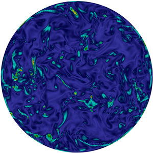
Figure 1 compares typical instantaneous experimental snapshots of the vorticity amplitude with the local energy transfer. This figure corresponds to a slice of an experimental measurement at scale $\ell =3.2\eta$ in the case T-$4$, while figure 2 comes from DNS data. As table 1 shows, these two cases share the same Reynolds number and resolution.

Figure 1.

Visualization of the vorticity amplitude $\omega$ (a) and $\mathscr {D}^{{I}}_{\ell }$ (b) for $\ell =3.2\eta$ for the case T-$4$ of table 1 in a plane containing the cylinder's axis.

Figure 2.

Visualization of the vorticity amplitude of $\omega$ (a) and $\mathscr {D}^{{I}}_{\ell }$ (b) for $\ell =8\eta$ on a plane containing the centre perpendicular to the cylinder's axis from the DNS of table 1.

Despite a higher level of noise in the local energy transfer fields, one observes a clear but not exact spatial correlation between location of high vorticity amplitude and high values of $\mathscr {D}^{{I}}_{\ell }$, as already noted in Saw et al. (Reference Saw, Kuzzay, Faranda, Guittonneau, Daviaud, Wiertel-Gasquet, Padilla and Dubrulle2016). In figure 2, we show an equivalent comparison between an instantaneous vorticity field and the local energy transfer, in a mid-height plane perpendicular to the rotation axis. As in the experimental case, we observe a spatial correlation between local maxima of vorticity and local energy transfer, but the correlation is not exact. To quantify further such correlation, we perform in the next section a detailed statistical analysis.

4.2. Joint statistics

Figure 3 (respectively figure 4) shows the joint probability distribution function (PDF) between the amplitude of the vorticity $\omega$ and the local energy transfer $\mathscr {D}^{{I}}_{\ell }$ at different scales, in the experiment T-$4$ (respectively in the DNS). Each PDF is computed over the available dataset which corresponds to the experimental cuboid for the experiment T-$4$, and to the entire tank, excluding the impellers for the DNS. Except for very large values of $\omega /\langle \omega \rangle$ and $\mathscr {D}^{{I}}_{\ell }/\epsilon$, all cases display a pyramidal correlation, similar to what was observed in Debue (Reference Debue2019) for the joint PDF between the local dissipation and the local energy transfer $\mathscr {D}^{{I}}_{\ell }$. This is not surprising, since dissipation and enstrophy are known to be correlated. The joint PDF of $({\mathscr {D}^{{I}}_{\ell }}/{\epsilon },{\omega }/{\langle \omega \rangle })$ shows that, for every scale, strong events of inter-scale transfer are associated with strong vorticity. In the inertial range (see figure 3b, respectively figure 4b), $\ell \gg \eta$, the PDF is tilted towards positive energy transfers, indicating that the energy is going down the scales. In the viscous range (see figure 3a, respectively figure 4a), the PDF seems to be symmetric with respect to the line $\mathscr {D}^{{I}}_{\ell }=0$. A marked discrepancy appears between the numerical results and the experiments when looking at high values of $\omega /\langle \omega \rangle$, since the joint PDF computed from the DNS exhibits a well-defined elongated feature, tracing a high degree of correlation between $\omega /\langle \omega \rangle$ and $\mathscr {D}^{{I}}_{\ell }/\epsilon$. We have investigated the spatial distribution of the events corresponding to this tail in an instantaneous snapshot. It is displayed in figure 5. We see that these events are organized into coherent structures, with three favoured locations: (i) at the blade forefront, in the impeller region, where each blade strongly pushes the flow; (ii) at the outer edge of the disk supporting the impeller; (iii) in two blobs that are lying near the cylinder edge, and just above or just below the middle shear layer. While the first two types of event can be associated with local gradient sources due to the impellers that are difficult to measure experimentally, the last category corresponds to the location of the strong vortices of the shear layer. The latter are known to be present in the von Kármán geometry (Ravelet, Chiffaudel & Daviaud Reference Ravelet, Chiffaudel and Daviaud2008) and they are the locus of strong energy transfers (Marie & Daviaud Reference Marie and Daviaud2004; Kuzzay, Faranda & Dubrulle Reference Kuzzay, Faranda and Dubrulle2015). This explains why such events have both strong vorticity, and strong local energy transfer. The absence of strong correlated events in the middle of the tank may explain why the joint PDF $\mathbb {P}({\mathscr {D}^{{I}}_{\ell }}/\epsilon ,{\omega }/{\langle \omega \rangle })$ based on experiment T-$4$ does not exhibit the tail, since the corresponding data were only taken in a small cube at the centre of the tank.

Figure 3.

Joint PDF of $\mathbb {P}({\mathscr {D}^{{I}}_{\ell }}/{\epsilon },{\omega }/{\langle \omega \rangle })$ for different scales from experimental measurements in table 1 computed over several uncorrelated snapshots. Here, $\omega$ refers to the norm of the vorticity, and $\mathscr {D}^{{I}}_{\ell }$ is the energy transfer. (a) T-$4$: $\ell =3.2 \eta$ ($3 \times 10^4$ snapshots). (b) T-$2$: $\ell =17.9\eta$ ($1.02\times 10^4$ snapshots). White colour corresponds to a lack of events in the dataset.

Figure 4.

Joint PDF of $\mathbb {P}({\mathscr {D}^{{I}}_{\ell }}/{\epsilon },{\omega }/{\langle \omega \rangle })$ for different scales from the DNS in table 1 computed over $21$ uncorrelated snapshots. Here, $\omega$ refers to the norm of the vorticity, and $\mathscr {D}^{{I}}_{\ell }$ is the energy transfer. A zoom on the central region is presented in each panel to compare with figure 3. (a) $\ell =1.06 \eta$; (b) $\ell =26.5\eta$. White colour corresponds to lack of events in the dataset.

Figure 5.

Positions of DNS points in the tail of figure 4(b) where $\mathscr {D}^{{I}}_{\ell } >\epsilon$ and $\omega > 5 \langle \omega \rangle$ for $\ell =26.5\eta$. The colours correspond to the $z$ values of the points, indicating that most of them are close to the impellers ($0.7<|z|<1.02$), or at the tank mid-height. This plot shows positions for one single snapshot.

Using the joint PDF, we have computed the conditional average $\mathbb {E}({\mathscr {D}^{{I}}_{\ell }}/{\epsilon }|{\omega }/{\langle \omega \rangle })$ as the average of ${\mathscr {D}^{{I}}_{\ell }}/{\epsilon }$ over the points where ${\omega }/{\langle \omega \rangle }$ is fixed. It is plotted on figure 6 as a function of $({\omega }/{\langle \omega \rangle })^2$ both in the numerical and experimental cases. For $\ell \sim \eta$, the conditional average $\mathbb {E}({\mathscr {D}^{{I}}_{\ell }}/{\epsilon }|{\omega }/{\langle \omega \rangle })$ increases almost linearly with $({\omega }/{\langle \omega \rangle })^2$. For large $\ell \gg \eta$ the conditional averages seem to reach a plateau where the local energy transfers do not depend anymore on the vorticity, meaning that there is no correlation at large scales. This feature is more pronounced in the DNS than in the experiment. This shows that local energy transfers and vorticity are only correlated at small scales.

Figure 6.

Conditional average $\mathbb {E}(\mathscr {D}^{{I}}_{\ell }|\omega )/\epsilon$ as a function of $(\omega /\langle \omega \rangle )^2$ for different scales $\ell$. They are computed from joint PDFs as in figures 3 and 4 from datasets of the DNS and cases T-$1$ to T-$4$ in table 1. Symbols are coded according to table 1.

In order to investigate the link between the energy transfers and velocity increments, the joint PDF of $\mathscr {D}^{{I}}_{\ell }$ with the full ($\delta W_{\ell }$) and anti-symmetric ($\delta \varOmega _{\ell }$) components of the velocity increments are plotted in figures 7 and 8. It appears that positive values of $\mathscr {D}^{{I}}_{\ell }$ are promoted for both quantities. In the inertial range, it seems that the large $\mathscr {D}^{{I}}_{\ell }$ are more correlated with strong events of $\delta \varOmega _{\ell }$ than with $\delta W_{\ell }$, since the PDF of $(\mathscr {D}^{{I}}_{\ell },\delta \varOmega _{\ell })$ is more tilted to the right-hand side, and most of the positive energy transfers are associated with increments of the order of several times the mean value.

Figure 7.

Joint PDF of $\mathbb {P}({\mathscr {D}^{{I}}_{\ell }}/{\epsilon },{\delta W_{\ell }}/{\langle \delta W_{\ell } \rangle })$ for different scales from the DNS in table 1 computed over $21$ uncorrelated snapshots. (a) $\ell =1.06 \eta$; (b) $\ell =26.5\eta$. White colour corresponds to lack of events in the dataset.

Figure 8.

Joint PDF of $\mathbb {P}({\mathscr {D}^{{I}}_{\ell }}/{\epsilon },{\delta \varOmega \ell }/{\langle \delta \varOmega \ell \rangle })$ for different scales from the DNS in table 1 computed over $21$ uncorrelated snapshots. (a) $\ell =1.06 \eta$; (b) $\ell =26.5\eta$. White colour corresponds to lack of events in the dataset.

4.3. Local energy transfers

We now focus on the scale behaviour of the statistical average of the local energy transfer $\mathscr {D}^{{I}}_{\ell }$, and the local energy dissipation $\mathscr {D}^{\nu }_{\ell }$. The comparison between numerical and experimental data is performed in figure 9(a). For each experimental dataset, a filtering process is applied to the data giving a range of accessible $\ell$ scaling from $\Delta x$ to approximately $10 \Delta x$ depending on the size of the PIV grid. Combining all datasets with accessible $R_{\lambda }$, $\epsilon$ and $\eta$ allows us to cover a wide range of scales in terms of ${\ell }/{\eta }$. They all behave according to the Kolmogorov 1941 phenomenology (Dubrulle Reference Dubrulle2019): the local energy transfer is much lower than the local energy dissipation for $\ell /\eta <10$ and saturates beyond a constant value, while the local energy dissipation decreases from the dissipative range to the large scales following a $\ell ^{-4/3}$ law. The agreement between experimental data and numerical data is very good for $\mathscr {D}^{\nu }_{\ell }$, but poor for $\mathscr {D}^{{I}}_{\ell }$. We assign such mismatch to convergence effects: indeed, even if our statistical samples are quite large, the presence of very large events in the local transfer that can be either positive or negative renders the statistics very difficult to converge. Note that $\mathscr {D}^{\nu }_{\ell }$ is mainly positive, so that the plots in figure 9(a) of $\langle \mathscr {D}^{\nu }_{\ell } \rangle$ and figure 9(b) of $\langle \vert \mathscr {D}^{\nu }_{\ell } \vert \rangle$ are almost the same. These plots show that the agreement is excellent between experimental and DNS data. In contrast, $\mathscr {D}^{{I}}_{\ell }$ takes extreme positive and negative values. We suspect that this is the reason why the statistics of $\langle \mathscr {D}^{{I}}_{\ell } \rangle$ in figure 9(a) are less well converged. To test this idea, we plot in figure 9(b) $\langle \vert \mathscr {D}^{{I}}_{\ell } \vert \rangle$, which shows that statistics are indeed improved. This issue is linked to the presence of rare events of extreme values of $\mathscr {D}^{{I}}_{\ell }$, as discussed in the appendix of Debue et al. (Reference Debue, Shukla, Kuzzay, Faranda, Saw, Daviaud and Dubrulle2018) for experimental points. A convergence study of the DNS statistics is presented in the appendix A (figure 15). On the other hand, the local dissipation, that is always positive, does not suffer from such drawback. To check such a hypothesis, we plot in figure 9(b) the average of the absolute values of $\mathscr {D}^{{I}}_{\ell }$ and $\mathscr {D}^{\nu }_{\ell }$. Indeed, we see that the data are less scattered, and that data points corresponding to different experiments follow a clear trend. The numerical data are closer to the TPIV data than the SPIV data. This might be due to the fact that SPIV data are 2-D–3C, meaning that some components of $\mathscr {D}^{{I}}_{\ell }$ are missing. These plots show that the ‘inertial range’ (location where $\mathscr {D}^{{I}}_{\ell }$ is constant) extends from $\ell /\eta =20$ to $\ell /\eta =100$ for the numerical data. Such observation will be used to compute the scaling exponents in § 4.6.

Figure 9.

Scale variation of the non-dimensional local energy transfer (red) and dissipation (green) for SPIV experiments A to E (filled symbols), TPIV experiments (open symbols) and the DNS (filled symbols with black line). Dotted lines correspond to $\ell ^{-4/3}$. Panel (a) for $\langle \mathscr {D}^{{I}}_{\ell }\rangle$ and $\langle \mathscr {D}^{\nu }_{\ell }\rangle$ non-dimensionalized by the total energy dissipation in the observational box; (b) same for absolute values. The symbols are coded according to table 1.

4.4. Structure functions

Longitudinal and wavelet velocity structure functions, as well as non-dimensional moments of $\mathscr {D}^{{I}}_{\ell }$, have been previously computed and discussed in Saw et al. (Reference Saw, Debue, Kuzzay, Daviaud and Dubrulle2018), Debue et al. (Reference Debue, Shukla, Kuzzay, Faranda, Saw, Daviaud and Dubrulle2018) and Dubrulle (Reference Dubrulle2019) from the experimental SPIV datasets A–E of table 1, with the drawback that the velocity field is only 2-D–3C. Here, we repeat their computation with experimental and numerical 3-D–3C data, with a focus on the wavelet velocity structure functions that are more appropriate for our purpose, see § 2.2. Figure 10(a) shows the comparison of the compensated wavelet velocity structure functions $\tilde {S}_W(p)=\langle \delta W_{\ell }^p\rangle /\langle \delta W_{\ell }^3\rangle ^{p/3}$ of orders $1$ to $6$ for numerical and experimental SPIV data. One sees that they are in good agreement for $p=1$ to $4$, and that the agreement deteriorates at large scales for higher $p$. This is probably due to a lack of convergence for the numerical data because of limited sampling. The same comparison has been done for the anti-symmetric wavelet velocity structure functions in figure 10(b), leading to a similar conclusion.

Figure 10.

Scale variation of the normalized non-dimensional wavelet structure functions of order $p=1$ to $p=6$ for SPIV experiments A to E (filled symbols) and the DNS (filled symbols with black line) The structure functions have been shifted by arbitrary factors for clarity and are coded by colour: $p=1$, blue symbols; $p=2$, orange symbols; $p=3$, yellow symbols; $p=4$, magenta symbols; $p= 5$, green symbols; $p=6$, light blue symbols. (a) Structure functions $\tilde S_W(p)$. (b) Structure functions for the anti-symmetric component $\tilde S_{\varOmega }(p)$. The dashed lines are power laws with exponents $\tau _W$ and $\tau _{\varOmega }$ shown in figure 13(a). The symbols are coded according to table 1.

Finally, we compare the compensated moments of the local energy transfer $\mathscr {D}^{{I}}_{\ell }$ for numerical and experimental data in figure 11(a). There is good agreement between numerical data and experiments in the inertial range, but not in the dissipative range or at large scales.

Figure 11.

(a) Scale variation of the compensated structure functions of the local energy transfer $\tilde S_D(p/3)$ of orders $p=1$ to $6$ for SPIV experiments A to E (filled symbols), TPIV experiments (open symbols) and the DNS (filled symbols with black line). The structure functions have been shifted by arbitrary factors for clarity and are coded by colour: $p=1$, blue symbols; $p=2$, orange symbols; $p=3$, yellow symbols; $p=4$, magenta symbols; $p= 5$, green symbols; $p=6$, light blue symbols. The dashed lines are power laws with exponents $\tau _D$ shown in figure 13(a). The symbols are coded according to table 1. (b) Parameter $\beta$ given in (4.1). Labels are taken according to table 1. The dotted line follows the equation $1/\beta = (4/3)\log (R_{\lambda })$.

4.5. Test of log universality

In figure 11(a), we compare the structure functions of the local energy transfer using data at different Reynolds numbers (see table 1). In agreement with the Kolmogorov self-similarity hypothesis, we can expect, and we indeed observe, that they have a universal behaviour in the inertial range, but not outside. As first discussed by Frisch & Vergassola (Reference Frisch and Vergassola1991) and Castaing, Gagne & Hopfinger (Reference Castaing, Gagne and Hopfinger1990), a more general log-universality property can be expected using the multi-fractal hypothesis, if one works with variables that are rescaled by a factor proportional to $\log (R_{\lambda })$, where $R_{\lambda }$ is the Taylor Reynolds number. In Geneste et al. (Reference Geneste, Faller, Nguyen, Shukla, Laval, Daviaud, Saw and Dubrulle2019), we have indeed shown that such a rescaling enables a better collapse of the velocity structure functions $S_W$, and linked such log universality with the extensivity of the large deviation function of the multi-fractal measure $\delta W_{\ell }^3/\langle \delta W_{\ell }^3\rangle$. If the local refined similarity hypothesis (2.9) holds true, one can expect that the log universality also applies to the measure $\vert \mathscr {D}^{{I}}_{\ell }\vert /\langle \vert \mathscr {D}^{{I}}_{\ell }\vert \rangle$, so that

(4.1)\begin{equation} \beta({Re})\left(\frac{\ln( \tilde S_D(p)/S_{0p})}{\ln(L_0/\eta)}\right)= F\left(p,\beta({Re})\frac{\ln(\ell/\eta)}{\ln(L_0/\eta)} \right). \end{equation}

We take the DNS at $R_{\lambda }=72$ as the reference case, and find, for both DNS and experiments, values of $\beta ({Re})$ and $S_{0p}$ that best collapse the curves. The corresponding collapses are provided in figure 12. The collapse is good for any value, except for the TPIV at the lowest Reynolds number, which does not collapse in the dissipative range. The collapsing curves display three different scaling regimes. At low $\ell /\eta$, a saturation can only be seen in the DNS, which corresponds to the far viscous range, where the velocity field becomes regular, so that $\langle \vert \mathscr {D}^{{I}}_{\ell }\vert ^p\rangle \sim \ell ^{2p}$ (Dubrulle Reference Dubrulle2019), and $S_D(p)\sim \mathrm {cte}$. In the inertial range, we observe a scaling $S_D(p)\sim \ell ^{\tau _D(p)}$ and in between, an intermediate range due to the random character of the dissipative scale, corresponding to the coexistence of regions of flow with different Hölder exponents, with areas where the flow has been relaminarized due to the action of viscosity (Geneste et al. Reference Geneste, Faller, Nguyen, Shukla, Laval, Daviaud, Saw and Dubrulle2019).

Figure 12.

Computation of (4.1) from order $p=1$ to order $p=6$. Collapse is observed for all experiments presented in table 1, using DNS (orange circles) as the reference and the $\beta$ parameter taken from figure 11(b).

The values of $\beta ({Re})$ are shown in figure 11(b). In agreement with previous results (Geneste et al. Reference Geneste, Faller, Nguyen, Shukla, Laval, Daviaud, Saw and Dubrulle2019), they collapse on a curve $1/\beta \sim (1/{\beta _0})\log (R_{\lambda })$, with $\beta _0\sim 3/4$ over the whole range of Reynolds numbers, and we do not observe the saturation of $1/\beta$ at low Reynolds numbers that is observed in the jet experiment of Castaing, Gagne & Marchand (Reference Castaing, Gagne and Marchand1993).

4.6. Scaling exponents and multi-fractal spectrum

Using the identification of the inertial range based on the local energy transfer (see § 4.3), we compute from figures 10 and 11 the scaling exponents $\tau _W(p)$, $\tau _{\varOmega }(p)$ and $\tau _D(p/3)$ for the numerical data. They are shown in figure 13(a). We see that $\tau _W(p)$ and $\tau _{\varOmega }(p)$ overlap in the range $p\in [-5, 5]$, and both overlap with $\tau _D(p/3)$ in the range $p \in [0,5]$, thereby validating the refined similarity hypothesis expressed by (2.9) (Dubrulle Reference Dubrulle2019). These overlapping values computed from numerical data compare very well with the value $\tau _W(p)$ computed on the SPIV data by Debue et al. (Reference Debue, Shukla, Kuzzay, Faranda, Saw, Daviaud and Dubrulle2018) and Dubrulle (Reference Dubrulle2019). We checked that the values of $\tau _D(p/3)$ coincide with the values obtained using figure 12. We also completed our measurements by computing more positive and negative moments, so as to be able to better estimate the multi-fractal spectra $C_W(h)$, $C_{\varOmega }(h)$ and $C_D(h)$ by Legendre transforms (see (2.13)). The resulting spectra are shown in figure 13(b). The two spectra $C_W(h)$ and $C_{\varOmega }(h)$ are parabolic, with a minimum shifted from $0$ by approximately $\delta h=0.08$. They are very close to each other for $h<0$ but differ more markedly for $h>0$, implying a different topology of regular regions. The value $C_W(h)=3$ or $C_{\varOmega }(h) =3$ extrapolated from the parabolic fit results in $h_{\mathrm {min}}\approx -0.53$. Using the shift property (2.14) and the measurement of $\zeta _W(3)=0.8$ (Dubrulle Reference Dubrulle2019), we can then estimate the most probable exponent for $\zeta _W$ and $\zeta _{\varOmega }$ as $0.35$, very close to the Kolmogorov value $0.33$. The minimum exponent for $C(h)$ is then $h_{min}=-0.26$. Note that the multi-fractal spectrum of the local energy transfer $C_D(3h)$ deviates strongly from the parabolic fit of $C_W(h)$, and displays a milder intermittency, as it is more peaked around the most probable value. This is not caused by insufficient statistics as the values of $\tau _D(p/3)$ are converged (see appendix A). It could be caused either by finite resolution (the finer scale is not small enough), meaning that we missed some very large energy transfers (Dubrulle Reference Dubrulle2019), or by a genuine difference between intermittency at very small scales caused by vorticity and the local energy transfer. To try to understand further the origin of intermittency, we then attempt another approach, based on conditional statistics.

Figure 13.

(a) Scaling exponents as a function of order for DNS (filled symbols with black outside) and SPIV (filled symbols): $\tau _W$, blue circles; $\tau _{\varOmega }$, red squares; $\tau _D$, yellow diamonds. (b) Corresponding multi-fractal spectrum $C(h)$ for the DNS scaling exponents. The spectrum has been obtained by taking the inverse Legendre transform of the scaling exponents $\tau (p)$ shown in figure 13(a). The dotted line curves are parabolic fit $C(h)=ah^2+bh+c$ with $a=8$ (respectively $9.5$), $b=-1.4$ (respectively $-1.2$) and $c=0.064$ (respectively $0.075$) for $C_W$ (respectively $C_{\varOmega }$).

4.7. Conditioned scaling exponents

To understand further the origin of intermittency, it is natural to condition the structure functions to areas of different values of the local energy transfer. An earlier attempt in that direction has been done in Debue et al. (Reference Debue, Shukla, Kuzzay, Faranda, Saw, Daviaud and Dubrulle2018), for the SPIV data, with the limitation that the conditioning could only be done on the local energy transfer at the smallest available scale of the dataset. Therefore, the conditioning was performed at the Kolmogorov scale only for the dataset E. The conclusion of such conditioning was that the intermittency was higher for areas corresponding to a larger (in absolute value) local energy transfer.

Using the data from the DNS, we can improve the procedure, by conditioning the structure functions at all scales by the local energy transfer at the Kolmogorov scale $\mathscr {D}^{{I}}_{\eta }$. Here, we enlarge the discussion by considering positive and negative values of the local energy transfer, as they may correspond to a different dynamics. Because of the conditioning, we have less statistics so we have to restrict ourselves to smaller values of $p$ than for unconditioned values. Once the structure functions have been conditioned, we can compute the corresponding conditioned scaling exponent by fitting power laws in the inertial range. The results for $S_W$ are shown in figure 14(a), for $p$ ranging from $0$ to $6$ and for centred reduced values of $\mathscr {D}^{{I}}_{\eta }$ ranging from $-5$ to $5$. One sees that for values $\mathscr {D}^{{I}}_{\eta }$ close to the mean, the scaling exponents are positive, and close to the Kolmogorov value $p/3$. For large negative $\mathscr {D}^{{I}}_{\eta }$, the scaling exponents are positive, but increase linearly with a small exponent $h_-\sim 0.1$. For large positive $\mathscr {D}^{{I}}_{\eta }$, the scaling exponents decrease quasi-linearly with a small exponent $h_+\sim -0.1$. This shows that negative local energy transfers are less intermittent than positive local energy transfers. The corresponding values of $h$ are close to $0$, reminiscent of shock-like structures. Exploring more singular structures closer to $h=-0.26$ (the minimum exponent of $C(h)$) would require a much larger number of statistics. We have repeated the analysis for the structure functions of the vortical part $S_{\varOmega }$ in figure 14(b). We observe a similar trend for large negative and positive values of $\mathscr {D}^{{I}}_{\eta }$, where we see that the scaling exponents are much more intermittent than for $\mathscr {D}^{{I}}_{\eta }$ around its mean value. In both cases, the conditioned exponent displays linear trends with $h_-\sim 0.1$ and $h_+\sim 0$, exponents that are close to their counterpart using $S_W$. Such a linear trend might be an indication that only one type of very singular structure is responsible for the scaling behaviour of $S_W$ or $S_{\varOmega }$ for large positive or negative local energy transfers.

Figure 14.

(a) Scaling exponent of the non-compensated wavelet structure functions $S_W$ computed using the joint PDF of the centred and reduced value of $\mathscr {D}^{{I}}_{\eta }$ and $\delta W_{\ell }$ at various scales $\ell$, and then a fit in the inertial range. The dotted lines have a slope of $-0.1$ for large positive values of centred and reduced value of $\mathscr {D}^{{I}}_{\eta }$, $1/3$ for small values of centred and reduced value of $\mathscr {D}^{{I}}_{\eta }$ and $0.1$ for large negative values of centred and reduced value of $\mathscr {D}^{{I}}_{\eta }$. (b) Same as (a), using the joint PDF of the centred and reduced value of $\mathscr {D}^{{I}}_{\eta }$ and $\delta \varOmega _{\ell }$. The dotted lines have a slope of $0$ for large positive values of centred and reduced value of $\mathscr {D}^{{I}}_{\eta }$, $1/3$ for small values of centred and reduced value of $\mathscr {D}^{{I}}_{\eta }$ and $0.1$ for large negative values of centred and reduced value of $\mathscr {D}^{{I}}_{\eta }$.