


1. Introduction
The laminar–turbulent transition of a separated shear layer is a fundamental problem in fluid dynamics. A flow can separate from the wall and generate a separation bubble either due to a large adverse pressure gradient or due to a sharp corner/blunt leading edge/rounded leading edge. A separation bubble generated due to a large adverse pressure gradient is termed a pressure-induced separation bubble (PISB), while a separation bubble generated due to a sharp corner/blunt leading edge/rounded leading edge is termed a geometry-induced separation bubble (GISB) in the literature (e.g. Diwan & Ramesh Reference Diwan and Ramesh2009; Robinet Reference Robinet2013; Yang Reference Yang2019). However, at a moderate Reynolds number, separation bubbles are characterized by the shear layer separation from the surface followed by the downstream reattachment onto the surface, which is believed to be due to the entrainment of turbulence in the shear layer (e.g. Dovgal, Kozlov & Michalke Reference Dovgal, Kozlov and Michalke1994; Tani Reference Tani1964).
The separation bubble emerges in many engineering devices, for example, in wind/gas turbine blades and in the wings of unmanned aerial and micro air vehicles. A separated flow on an aerodynamic body can adversely affect its aerodynamic performance. There have been considerable efforts to understand the dynamics of various separated flows. Nonetheless, several points that are not well understood, need further attention. For example, the effect of upstream turbulence on the dynamics of a turbulent separation bubble, which may also develop instabilities leading to coherent structures, is still not answered, and the separated flows often being noise amplifiers, their dynamics may be susceptible to different upstream conditions, the sensitivity of which is not clear (Robinet Reference Robinet2013). Similarly, the effect of upstream turbulence on the dynamics of a laminar separation bubble is not very clear.
Recently, there has been a renewed interest on the effect of free-stream turbulence (FST) on a separation bubble. Some recent studies (Balzer & Fasel Reference Balzer and Fasel2016; Stevenson, Nolan & Walsh Reference Stevenson, Nolan and Walsh2016) reported that the Klebanoff mode, as seen in the case of an attached boundary layer at an enhanced level of FST, is also found to exist for some geometry- and pressured-induced bubbles. On the other hand, for a GISB case, there can be a very short distance for the development of an attached boundary layer or no distance at all for the development of a boundary layer before the point of separation (Yang Reference Yang2019). A question then arises whether the Klebanoff mode can still be a flow feature for all the GISB cases or not. This is yet to be addressed and answered. This can be better addressed if a comparative experimental investigation on the response of a GISB and a PISB at an enhanced level of FST can be carried out.
1.1. Geometry-induced separation bubble
Various works on GISBs were carried out in the past focusing on several aspects, such as the reattachment length, low-frequency unsteadiness, vortex shedding and three-dimensional (3-D) flow features in the separated region (e.g. Lane & Loehrke Reference Lane and Loehrke1980; Ota, Asano & Okawa Reference Ota, Asano and Okawa1981; Kiya & Sasaki Reference Kiya and Sasaki1983b; Sasaki & Kiya Reference Sasaki and Kiya1991). In their experimental study, Kiya & Sasaki (Reference Kiya and Sasaki1983b) investigated the shedding characteristics of a separation bubble at the blunt leading edge of a flat plate and observed that the regular vortex shedding exists along with low-frequency unsteadiness. Such low-frequency oscillations due to large-scale unsteadiness in a separation bubble generated at the blunt leading edge are further reported experimentally and numerically by various authors (e.g. Cherry, Hillier & Latour Reference Cherry, Hillier and Latour1984; Tafti & Vanka Reference Tafti and Vanka1991; Yang & Voke Reference Yang and Voke2001). Using 3-D numerical simulation, Tafti & Vanka (Reference Tafti and Vanka1991) postulated that the low-frequency unsteadiness is due to the periodic enlargement and shrinkage of the separation bubble, caused by the mass buildup within the bubble and venting of the fluid in the spanwise direction, respectively.
Vortex shedding followed by the 3-D aspects of a separated shear layer has also been studied in various numerical and experimental works (e.g. Sasaki & Kiya Reference Sasaki and Kiya1991; Tafti & Vanka Reference Tafti and Vanka1991; Yang & Voke Reference Yang and Voke2001; Chaurasia & Thompson Reference Chaurasia and Thompson2011; Thompson Reference Thompson2012). Using flow visualization for a separation bubble at a blunt leading edge, Sasaki & Kiya (Reference Sasaki and Kiya1991) reported that, in the range of  $320< Re<380$, the shear layer rolls up to form aligned (in-phase) $\varLambda$-shape vortices shortly downstream of the reattachment line, whereas these are found to be in a staggered arrangement in the longitudinal direction for $Re>380$; here $Re$ is the Reynolds number based on the plate thickness. The numerical simulation of Yang & Voke (Reference Yang and Voke2001) reveals that the separated shear layer initially becomes unstable due to the Kelvin–Helmholtz (KH) instability and forms a two-dimensional (2-D) vortex followed by 3-D motions further downstream due to secondary instability, which eventually leads to a hairpin-like vortex before reattachment with the wall. In his transient growth analysis of this flow, Thompson (Reference Thompson2012) found the optimal perturbation field to be localized near the leading edge. Interestingly, his analysis on the effect of noise reveals that a very small noise level (0.1 %) can lead a steady separation bubble to an unsteady one because of substantial amplification of optimal modes.
To investigate the response of FST on a separation bubble at the blunt leading edge of a flat plate, Hillier & Cherry (Reference Hillier and Cherry1981) carried out surface pressure measurements at various FST levels. They found that the mean flow strongly responds to FST, whereas unsteady characteristics strongly depend on both FST and integral scales. Similarly, Castro & Haque (Reference Castro and Haque1988) found enhancements of the flapping motion of a separated shear layer at an enhanced level of FST. A separation bubble generated by a rounded leading edge of a flat plate at an enhanced level of FST was also investigated by Stevenson et al. (Reference Stevenson, Nolan and Walsh2016), who found that laminar streaks co-exist with the shedding structure in the separated shear layer, and the shedding structure contributes to the Reynolds stress production in the rear part of the bubble.
Towards finding the frequency spectra, Halfon et al. (Reference Halfon, Nishri, Seifert and Wygnanski2004) carried out hot-wire measurements of a separation bubble formed near the leading edge of an elliptic flat plate for different levels of FST and periodic excitation. At low FST levels, clear peaks in the frequency spectra were observed, indicating the presence of the KH instability mechanism, whereas, for high FST cases, no clear peak was observed. Similarly, Langari & Yang (Reference Langari and Yang2013) reported that the faster growth of turbulence kinetic energy accelerates the transition process and bypasses the KH instability mechanism at a higher level of FST. In contrast, the numerical simulations of Yang & Abdalla (Reference Yang and Abdalla2005) and Yang & Abdalla (Reference Yang and Abdalla2009) reveal that the addition of FST does not alter the shedding frequency of the separated shear layer. This contrasting viewpoint on the existence of a peak in the spectra certainly invites further studies on the effect of FST on a GISB.
1.2. Pressured-induced separation bubble
As compared with the GISB cases, there have been considerable studies on the PISB cases, as Tani (Reference Tani1964) reviewed some early works on this subject. Various works on a PISB indicate that disturbance grows exponentially in the separated shear layer and eventually leads to the shear layer roll-up (e.g. Gaster Reference Gaster1967; Pauley, Moin & Reynolds Reference Pauley, Moin and Reynolds1990; Watmuff Reference Watmuff1999; Häggmark, Bakchinov & Alfredsson Reference Häggmark, Bakchinov and Alfredsson2000; Lang, Rist & Wagner Reference Lang, Rist and Wagner2004). Using the laser-Doppler anemometry and the particle image velocimetry (PIV) techniques, Lang et al. (Reference Lang, Rist and Wagner2004) carried out a controlled experimental investigation in a PISB and compared their measured data with the linear stability theory and the direct numerical simulation. Their study reveals that transition is driven by a convective amplification of 2-D Tollmien–Schlichting (TS) waves, and the initial level of steady 3-D disturbances does not play a major role in the transition process. Similarly, for a separation bubble on an airfoil, Boutilier & Yarusevych (Reference Boutilier and Yarusevych2012) found their measured growth rate, wavenumber and convection velocity to compare well with the prediction of linear stability analysis (LSA). In their combined experimental and theoretical study, Diwan & Ramesh (Reference Diwan and Ramesh2009) found that the primary instability mechanism in a separation bubble is inflectional in nature, which originates at the upstream of the separation location. They also proposed a new scaling relation for the most amplified frequency for a wall-bounded shear layer in terms of the inflection-point height and the vorticity thickness. Several studies (e.g. Spalart & Strelets Reference Spalart and Strelets2000; Marxen et al. Reference Marxen, Lang, Rist, Levin and Henningson2009; Marxen, Lang & Rist Reference Marxen, Lang and Rist2013) are also carried out to understand the 3-D aspect of the separated shear layer transition. In the case of a forced laminar separation bubble, Marxen et al. (Reference Marxen, Lang and Rist2013) reported that an elliptic instability of the vortex core is responsible for the spanwise deformation, whereas a flow instability between two adjacent vortices is responsible for three dimensionality in the braid region.
Besides these controlled studies, the response of a separation bubble to an enhanced level of FST has also been investigated numerically and experimentally by various researchers. In his experimental work on the separation bubble under low-pressure turbine conditions at low (0.5 %) and high (9 %) FST levels, Volino (Reference Volino2002) found clear sharp spectral peaks for the low FST case, which led him to suggest TS instability mechanism for shear layer breakdown. For high FST levels, although he found the broadband spectrum, the peak was found to be at same the frequency as that of the low FST case, suggesting the possibility of TS transition even at high FST. Using the PIV technique, Simoni et al. (Reference Simoni, Lengani, Ubaldi, Zunino and Dellacasagrande2017) carried out an experimental study on PISB for various Reynolds numbers and FST levels. They found that the vortex shedding frequency does not change considerably with increasing the FST level. Similarly, Istvan & Yarusevych (Reference Istvan and Yarusevych2018) experimentally studied the effects of FST on transition in a laminar separation bubble over a NACA 0018 airfoil using the PIV technique. They reported that the spanwise vortices originate from the shear layer roll-up for all the FST levels (0.06 %–1.99 %). However, they found that the spanwise coherence reduces significantly with increasing FST levels, and the streamwise streak of low-speed fluid at the highest level of FST (1.99 %) leads to highly 3-D shear layer roll-up.
In their numerical simulation, Balzer & Fasel (Reference Balzer and Fasel2016) found a constant shedding frequency at enhanced levels of FST and the vortex shedding is not bypassed in the flow. Furthermore, their study reveals that there exists the streamwise algebraic/transient growth in the fore part of the bubble, followed by an exponential growth; the streamwise algebraic growth is attributed to the streamwise streaks (Klebanoff mode, hereafter referred to as the K mode), whereas the exponential growth is due to the KH mode. Their LSA confirms that the primary linear stage of the transition mechanism (KH instability) is not bypassed even at an enhanced level of FST. A recent numerical study by Hosseinverdi & Fasel (Reference Hosseinverdi and Fasel2019) reveals that the K mode can emerge in the flow even at a smaller level of FST. Nevertheless, the transition is dominated by a 2-D mode (KH mode). When the FST level increases, both the K mode and the KH mode contribute to the transition mechanism. Similarly, in their large eddy simulation in a PISB in the presence of FST, Li & Yang (Reference Li and Yang2019) reported that there exist two transition mechanisms, i.e. K-mode and KH-mode instability mechanisms. Their numerical flow visualization reveals that the spanwise 2-D rollers are severely distorted due to high FST, leading to highly 3-D rollers without any clear spectral peak associated with the KH instability. Nonetheless, the small peaks at different frequencies in their spectral analysis of the streamwise velocity data are reported to be associated with the shedding of the disrupted 2-D rollers, which may be a manifestation of the KH instability. However, they concluded that the KH instability mechanism is not the dominant mechanism at the FST level of 2.9 %. In their direct numerical simulation, McAuliffe & Yaras (Reference McAuliffe and Yaras2010) found that clear spectral peaks are absent in the bubble region at the FST level of 1.45 %. Moreover, they reported that the streamwise streaks in the flow bypass the shear layer roll-up process, indicating that the primary KH instability mechanism leading to shear layer roll-up is bypassed, although they found this mechanism to be active at the secondary instability stage during turbulent spot formation.
1.3. Aims of the present study
The above reviews clearly indicate some contrasting observations on the presence of vortex shedding frequency and the instability mechanism in a separated shear layer at an enhanced level of FST. Some studies (e.g. Yang & Abdalla Reference Yang and Abdalla2005, Reference Yang and Abdalla2009; Balzer & Fasel Reference Balzer and Fasel2016) indicate that the primary linear stage of the transition mechanism (KH instability) is not bypassed even at an enhanced level of FST, whereas some authors (e.g. McAuliffe & Yaras Reference McAuliffe and Yaras2010; Langari & Yang Reference Langari and Yang2013) concluded that the primary instability mechanism is bypassed, as they did not find any clear peak in the streamwise fluctuating velocity ( $u$) spectra. An obvious question then is to ask: Can we come to a conclusion about the existence/non-existence of the primary instability mechanism based on the presence/absence of a spectral peak in the $u$ velocity signal? If the spectral peak does not exist in the $u$ velocity spectra or if it does not remain constant at an enhanced level of FST while other conditions remain the same, can the LSA even then describe the disturbance evolution in the separated flows?
Some works also reveal co-existence of both the K mode and KH mode in a separation bubble at an enhanced level of FST (e.g. Stevenson et al. Reference Stevenson, Nolan and Walsh2016; Hosseinverdi & Fasel Reference Hosseinverdi and Fasel2019; Li & Yang Reference Li and Yang2019). Then, another legitimate question which arises: Is this feature universal for all types of separation bubble? If both the K mode and KH mode are present, what role does the K mode/a streaky structure play in flow transition in a separated flow?
Therefore, the present comparative study is aimed at answering these above questions considering both the geometry-induced and pressure-induced separation bubbles. This paper is organized as follows. Details of the experimental set-ups and the measurement techniques are described in § 2, followed by the data analysis techniques in § 3. The results are presented in § 4. The summary of the results followed by a concluding remark is presented in § 5.
2. Experimental details
2.1. Wind tunnels and set up for separation bubbles
The present measurements were carried out in a low-turbulence and low-speed wind tunnel. The settling chamber of the open-return, suction-type wind tunnel houses a honeycomb section (30 mm long) and six turbulence reduction screens, followed by a contraction cone with a contraction ratio of  $16:1$. The tunnel has a square test section of dimensions 610 mm $\times$ 610 mm; the length of the test section is 3000 mm. The test section is followed by a long diffuser. A fan at the diffuser end is driven by a 15-hp motor, which is controlled by a speed controller (made by Siemens). The streamwise FST intensity in the empty test section is 0.1 % of the free-stream velocity (Balamurugan & Mandal Reference Balamurugan and Mandal2017).
A transparent acrylic flat plate with a blunt leading edge (right-angled corners) was used for generation of a GISB (e.g. Hillier & Cherry Reference Hillier and Cherry1981; Kiya & Sasaki Reference Kiya and Sasaki1983a), as schematically shown in figure 1(a). On the other hand, a contoured wall in the test section (e.g. Häggmark et al. Reference Häggmark, Bakchinov and Alfredsson2000; Marxen et al. Reference Marxen, Lang, Rist and Wagner2003; Diwan & Ramesh Reference Diwan and Ramesh2009), as shown in figure 1(b), was used to generate a PISB on a horizontal flat plate with an asymmetrical modified super elliptic leading edge. The present pressure gradient set-up is a slightly modified version of that used by Dhiman (Reference Dhiman2015). The contoured wall, which was made of wood, was 1500 mm long and 610 mm wide with a maximum depth of 165 mm. The profile for the contoured wall in the favourable pressure gradient region was obtained from a fifth degree polynomial,  $y_a=ax_{a}^{5}+bx_{a}^{4}+cx_{a}^{3}+dx_{a}^{2}+ex_{a}$, where $a$,
$a$,  $b$,
$b$,  $c$,
$c$,  $d$ and $e$ are constants. Here, the origin, i.e. $x_a$ = 0 and $y_a$ = 0, is located at the starting of the contoured wall from the top wall of the tunnel; $x_a$ is positive in the flow direction, whereas $y_a$ is positive upward. The numerical values of the constants $a$,
$a$,  $b$,
$b$,  $c$,
$c$,  $d$ and $e$ are $-7.137\times 10^{-7}$, $8.263\times 10^{-8}$, $-2.734\times 10^{-5}$, 0.00158, $-0.01324$, respectively. Other portions of the contoured wall are straight lines. The boundary layer on the contoured wall was tripped to avoid flow separation on the contoured wall. A slot of 10 mm wide was made along the centreline of the contoured wall to facilitate the hot wire and the PIV measurements in the wall-normal plane. Both the plates were horizontally mounted in the mid-plane of the tunnel test section. The thickness of both the plates, denoted by $h$, was 12 mm. The plates with blunt and asymmetrical modified super elliptic leading edges were 1500 and 1800 mm long, respectively. The present asymmetric modified super elliptic leading edge was designed and fabricated following the work of Hanson, Buckley & Lavoie (Reference Hanson, Buckley and Lavoie2012), with a thickness ratio of 7/24 between the working and non-working sides. The leading edge was 120 mm long. The aspect ratios for the upper and lower ellipses were 34.3 and 14.1, respectively. Hanson et al. (Reference Hanson, Buckley and Lavoie2012) reported that this type of leading edge could reduce the receptivity of the boundary layer by eliminating the discontinuity at the juncture between the curved and the flat surfaces. Various studies in the literature considered flat plates with an asymmetric leading edge for reducing the pressure gradient around the leading edge region (e.g. Fransson, Matsubara & Alfredsson Reference Fransson, Matsubara and Alfredsson2005; Li & Gaster Reference Li and Gaster2006).
Simple sketches illustrating the arrangements for measurements in the wall-normal plane. (a) A blunt plate with right-angled corners for the generation of a GISB. (b) Contoured wall for generating a PISB over a flat plate with an asymmetric modified super elliptic leading edge.

To increase the turbulence level in the test section, a passive grid was installed at the entrance of the test section. We used two different passive grids. These grids, denoted as grid A and grid B, were bi-plane square grids made of circular and square bars of mild steel, respectively. The diameter of the circular bars and the mesh width of grid A were 5 and 72 mm, respectively, whereas grid B was made of 10 thick square bars with 45 mm mesh width. The solidity of grid A was 0.134, whereas it was 0.39 for grid B. The turbulence generated by these grids was nearly isotropic. The streamwise turbulence intensities were found to be 2.1 % and 3.3 % for grid A and grid B, respectively, at the flat plate leading edge, which was approximately 20 $M$ downstream of the grid location; here $M$ refers to the mesh width of a grid. The longitudinal integral length scales and the Taylor microscales were found to be 11.1 mm and 3.8 mm, respectively, for grid A, and 20.2 mm and 5.2 mm, respectively, for grid B. Further details, such as transverse integral length scales and the isotropic nature of the grid turbulence, are available in Aniffa (Reference Aniffa2023).
2.2. Measurements techniques
The PIV technique has extensively been used to measure the flow field in both the wall-normal ( $x\unicode{x2013}y$) and spanwise ( $x\unicode{x2013}z$) planes; here, the streamwise, wall-normal and spanwise directions are denoted by $x$,
$x$,  $y$ and $z$, respectively, and the corresponding fluctuating velocities in those directions are denoted by $u=U-U_{I}$, $v=V-V_{I}$ and $w = W-W_{I}$, respectively, where the corresponding uppercase quantities without suffix $I$ and with suffix $I$ are the mean and instantaneous velocities, respectively. We may note that $x = 0$ refers to the origin of the leading edge of the flat plate. Measurements have been carried out using a conventional 2-D PIV system (data acquisition rate $\leq$ 10 Hz), and a time-resolved PIV (TR-PIV) system (data acquisition rate $\sim$1 kHz). Three different cameras were utilized in the present investigation. A high-resolution CCD camera (TSI, USA, $4912\times 3280$ pixels, frame rate in double frame mode 1 Hz) was used for the conventional 2-D PIV system. Two different CMOS cameras, one with a resolution of $2560\times 1920$ pixels (CMOS-1) and another with a resolution of $3840 \times 2400$ pixels (CMOS-2), were utilized in this work. Both of these cameras were procured from IDTvision, USA. The maximum frame rates at the maximum resolutions in double exposure mode are 365 and 500 Hz for the CMOS-1 and CMOS-2 cameras, respectively. It should be noted that all the TR-PIV measurements for the GISB and PISB cases were carried out using CMOS-1 and CMOS-2 cameras, respectively. A macro planner lens of 100 mm focal length (Carl Zeiss) was used with these cameras for data acquisition. Two laser units, i.e. a double pulsed Nd:YAG laser (InnoLas Laser GmbH, Germany, SpitLight Compact 400, energy $180$ mJ per pulse at 532 nm, repetition rate $10$ Hz), and a high-frequency double pulsed Nd:YLF laser (Photonics Industries, dual head DPSS, energy $30$ mJ per pulse at 527 nm till the repetition rate of $1$ kHz) were used for illumination. Using sheet forming optics and articulated light arms (procured from Laser and Imaging Sciences, UK, and ILA Intelligent Laser Applications GmbH, Germany), a thin laser sheet of approximately 1 mm thickness was produced and delivered to the measurement plane. The flow was seeded with fog particles of a mean diameter of approximately $1\,\mathrm {\mu }$m using a fog generator (SAFEX fog generator, Dantec Dynamics, Denmark). It was placed ahead of the tunnel entrance, and a uniform distribution of fog particles was ensured using a small fan, as was done in our previous work in this tunnel (e.g. Balamurugan & Mandal Reference Balamurugan and Mandal2017; Balamurugan et al. Reference Balamurugan, Rodda, Philip and Mandal2020). The laser and the camera were synchronized using the MotionPro timing unit (IDTpiv, USA) and the TSI synchronizer (TSI, USA). A simple sketch illustrating arrangements for the PIV measurements in the $x\unicode{x2013}y$ plane for both the GISB and PISB cases is shown in figures 1(a) and 1(b), respectively.
Before proceeding with the PIV measurements, the separation bubble region was identified using the smoke flow visualization technique. Since the separated region for a GISB was found to be comparatively small, the CMOS camera was used for both the conventional and the TR-PIV measurements with regions of interest in the ( $x\unicode{x2013}y$) plane of $113\ {\rm mm}\times 85$ and $100\ {\rm mm}\times 42\ {\rm mm}$, respectively; we may note that the region of interest for the TR-PIV measurements was chosen to be less than the conventional measurements to increase the acquisition rate. Similarly, the conventional and TR-PIV measurements were carried out for a PISB in the ( $x\unicode{x2013}y$) plane. As the separated region was found to be large in a PISB, a high-resolution CCD camera was used to cover $310\ {\rm mm}\times 207\ {\rm mm}$ in the ( $x\unicode{x2013}y$) plane for better spatial resolution. On the other hand, the TR-PIV measurements in the ( $x\unicode{x2013}y$) plane for a PISB were carried out covering $158\ {\rm mm}\times 89\ {\rm mm}$ around the maximum height of the bubble for the comparable spatial resolution. The conventional PIV measurements using the CCD camera in the ( $x\unicode{x2013}z$) plane were also carried out at $y$ = 2 mm height from the surface, for both the GISB and PISB cases, with regions of interest of $201\ {\rm mm}\times 134\ {\rm mm}$ and $258\ {\rm mm}\times 172\ {\rm mm}$, respectively. Sufficient numbers of realizations were acquired for both the PISB and GISB cases, as detailed in the following section. The TR-PIV data were acquired at 645 Hz, i.e. 645 image pairs per second, for the GISB cases, whereas the TR-PIV data were acquired at 500 Hz for the PISB case. Similarly, the conventional measurements were acquired at a rate of 1 Hz, except for the conventional measurements in the $(x\unicode{x2013}y)$ plane for a GISB, which were carried out at a rate of 10 Hz. However, the acquired images were processed using the mess-free software, ProVision XS (IDTpiv), with a correlation window of 32 pixels $\times$ 32 pixels. The package, ProVision XS, includes a feature for high spatial resolution, details of which can be found in the literature (Lourenco & Krothapalli Reference Lourenco and Krothapalli2000; Alkislar, Krothapalli & Lourenco Reference Alkislar, Krothapalli and Lourenco2003). This package was also used in various previous works (e.g. Mandal, Venkatakrishnan & Dey Reference Mandal, Venkatakrishnan and Dey2010; Balamurugan & Mandal Reference Balamurugan and Mandal2017). The uncertainty analysis of the PIV measurements was performed following our previous work (Balamurugan & Mandal Reference Balamurugan and Mandal2017). We considered the uncertainty due to particle displacement, alignment of the calibration target and time delay of the signal (Gui & Wereley Reference Gui and Wereley2002; Holman Reference Holman2012; Thielicke Reference Thielicke2014; Coleman & Steele Reference Coleman and Steele2018; Raffel et al. Reference Raffel, Willert, Scarano, Kähler, Wereley and Kompenhans2018). The estimated maximum uncertainties in the velocity are found to be ${\pm }1.5\,\%$ and ${\pm }2.6\,\%$ of the free-stream velocity for the GISB and PISB cases, respectively. A hot-wire anemometry system procured from Dantec Dynamics, Denmark, was also used in this present study. A single hot-wire probe (55P11, Dantec Dynamics) was used for data acquisition. The sensing element was 5 $\mathrm {\mu }$m diameter tungsten wire with a length to diameter ratio of 250. The data were acquired using a 16 bit NI data acquisition card and the LabVIEW software with a sampling rate of 6 kHz. For measuring the free-stream turbulent intensity, the probe was calibrated using a Pitot static tube and the King's law fit. The uncertainty in the mean velocity measured by the hot-wire system is estimated following the works of Yavuzkurt (Reference Yavuzkurt1984) and Balamurugan & Mandal (Reference Balamurugan and Mandal2017). The estimated uncertainty is found to be less than ${\pm }2.5\,\%$.
2.3. Velocity and pressure distributions
The coefficient of pressure,  $C_{p}$ $(=1-({U_{e}^2+V_{e}^2})/{U_{r}^2})$, for the GISB cases, was determined from the streamwise edge velocity ( $U_{e}$) and the wall-normal edge velocity ( $V_{e}$) of the separated shear layer, whereas the coefficient of pressure, $Cp$
$Cp$  $(=1-{U^2}/{U_{r}^2})$, for the PISB cases were determined from the mean velocity measured outside of the separation bubble; here, the reference velocity, $U_{r}$, is considered as the mean velocity at $x=-220$ mm from the plate leading edge, such that this location is well ahead of the converging section of the contoured wall, and the edge velocity, $U_{e}$, is considered as the mean velocity at the shear layer edge. However, for the GISB cases, $U_{e}$ and $V_{e}$ were obtained from the PIV measurements in the wall-normal plane. For the PISB cases, such PIV measurements over the entire length of the pressure gradient set-up were not possible. Therefore, the hot-wire measurements were carried out to determine the mean velocity for the PISB cases. The measurements were carried out at various streamwise locations while keeping the probe at a wall-normal location higher than the maximum height of a PISB. The hot-wire data were acquired at a rate of 6 kHz.
Variations of  $U_{e}/U_{r}$ and $C_p$ distributions along the streamwise direction are shown in figures 2(a) and 2(b), respectively, for the GISB cases. Similarly, figures 2(c) and 2(d) show $U/U_{r}$ and $C_{p}$ distributions, respectively, for the PISB cases. It should be noted that GISB-N2 and GISB-B2 in these figures denote measurements with no grid and grid B at $U_{r} = 2\ {\rm m}\ {\rm s}^{-1}$ for the GISB cases; similarly, PISB-N2 and PISB-B2 denote measurements with no grid and grid B at $U_{r} = 2\ {\rm m}\ {\rm s}^{-1}$ for the PISB cases; the hot-wire measurements along the streamwise direction were carried out keeping the hot-wire probe at $y/h = 1.25$ and $y/h = 0.5$ for the PISB-N2 and PISB-B2 cases, respectively. The flow for the GISB cases is seen to accelerate initially before it decelerates in the downstream, although the flow separates at the blunt leading edge (with right-angled corners). Furthermore, the increase in the edge velocity is found to be more for an enhanced level of FST, i.e. for the GISB-B2 case as compared with the GISB-N2 case. This is attributed to the fact that the mean velocity around the point of separation is no more parallel to the streamwise direction, as the flow separates at an angle at the corner of the blunt leading edge (see figure 3 in § 4). This leads to the non-zero value of the wall-normal mean velocity, $V$, which is found to be higher for the GISB-N2 case as compared with the GISB-B2 case. As a result, the streamwise component of the mean velocity, i.e. $U_{e}$, is found to be less for the GISB-N2 compared with the GISB-B2 case for a given reference velocity, $U_{r} = 2\ {\rm m}\ {\rm s}^{-1}$. For the PISB cases, the flow in the converging section of the contoured wall accelerates as expected, followed by a deceleration in the diverging section. Moreover, the streamwise distributions of $U/U_{r}$ and $C_{p}$ for the PISB-N2 and PISB-B2 cases are nearly similar before the point of separation, as the mean flow is nearly parallel (see figure 4 in § 4). The $U/U_{r}$ variation in figure 2(c) is found to be similar to the velocity distribution reported in the literature (e.g. Häggmark et al. Reference Häggmark, Bakchinov and Alfredsson2000; Li & Yang Reference Li and Yang2019; Coull & Hodson Reference Coull and Hodson2011) for the PISB cases. The sudden drop in the value of $C_p$ in the range of $50< x/h<60$ in figure 2(d) indicates the transition in the separated shear layer (e.g. Häggmark et al. Reference Häggmark, Bakchinov and Alfredsson2000; Boutilier & Yarusevych Reference Boutilier and Yarusevych2012; Balzer & Fasel Reference Balzer and Fasel2016).
(a,b) Plots of  $U_{e}/U_{r}$ and $C_p$ distributions along the streamwsie direction, respectively, for different GISB cases. Symbols: ${--\circ --}$, red, GISB-N2 case; ${--\triangle --}$, red, GISB-B2 case. (c,d) Plots of $U/U_{r}$ and $C_p$ distributions along the streamwsie direction, respectively, for different PISB cases. Symbols: ${--\circ --}$, blue, PISB-N2 case measured at $y/h = 1.25$; ${--\triangle --}$, blue, PISB-B2 case measured at $y/h = 0.5$; here GISB-N2 and GISB-B2 refer to measurements at $U_{r} = 2\ {\rm m}\ {\rm s}^{-1}$ for no grid and grid B, respectively, for the GISB cases; PISB-N2 and PISB-B2 refer to measurements at $U_{r} = 2\ {\rm m}\ {\rm s}^{-1}$ for no grid and grid B, respectively, for the PISB cases, as further detailed in table 1.

Ensemble-averaged velocity vectors plotted over the contour of  $u_{rms}/U_{r}$. Symbols: —, $U = 0$ line; – – –, mean dividing streamline; ——, cyan, displacement thickness ( $\delta ^*$); $\circ$, location of the inflection points. Results are shown for the (a) GISB-N1 case, (b) GISB-A1 case, (c) GISB-B1 case, (d) GISB-N2 case, (e) GISB-A2 case, ( f) GISB-B2 case.

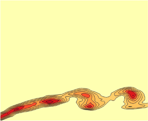
Ensemble-averaged velocity vectors plotted over the contour of  $u_{rms}/U_{r}$ for PISB cases. Symbols: —, $U = 0$ line; – – –, mean dividing streamline; ——, cyan, displacement thickness ( $\delta ^*$); $\circ$, location of the inflection points. Results are shown for the (a) PISB-N2 case, (b) PISB-A2 case, (c) PISB-B2 case.

3. Data analysis techniques
In this section we briefly describe the major data analysis tools, i.e. the proper orthogonal decomposition (POD) and LSA techniques.
3.1. The POD technique
The POD technique provides a set of orthogonal basis functions,  $\boldsymbol {\varPhi (x)}$, which can be used to decompose the fluctuating velocity field, $\boldsymbol {v(x)}$, as follows (Baltzer & Adrian Reference Baltzer and Adrian2011; Berkooz, Holmes & Lumley Reference Berkooz, Holmes and Lumley1993):
 \begin{equation} \boldsymbol{v}(\boldsymbol{x},t_{m})= \sum_{n}a^{n}(t_{m}) \boldsymbol{\varPhi}^{n}(\boldsymbol{x}). \end{equation}
Here the coefficients,  $a^{n}(t_{m})$, can be obtained by the following inner product:
 \begin{equation} a^{n}(t_{m}) = (\boldsymbol{v}(\boldsymbol{x},t_{m}), \boldsymbol{\varPhi}^{n}(\boldsymbol{x})). \end{equation}
The basis function,  $\boldsymbol {\varPhi (x)}$, to be an optimum one, should satisfy the following integral eigenvalue equation (Berkooz et al. Reference Berkooz, Holmes and Lumley1993):
 \begin{equation} \int_{\varOmega} \boldsymbol{R(x;x')} \boldsymbol{\varPhi(x')}\,{{\rm d} x}'= \lambda \boldsymbol{\varPhi}(\boldsymbol{x}). \end{equation}
Here  $\boldsymbol {R(x;x')}=\langle \boldsymbol {v(x)}\boldsymbol {v}^{*}\boldsymbol {(x')}\rangle$ represents a two-point correlation and $\varOmega$ denotes the domain of integration. The normalized basis functions are obtained such that $(\boldsymbol {\varPhi }^{m},\boldsymbol {\varPhi }^{n})=$ $\delta _{mn}$, where $\delta _{mn}$ is the Kronecker delta.
Using ‘the method of snapshot’ proposed by Sirovich (Reference Sirovich1987), POD basis functions are usually calculated from discrete PIV data (e.g. Kruse, Gunther & Rohr Reference Kruse, Gunther and Rohr2003; Meyer, Pedersen & Özcan Reference Meyer, Pedersen and Özcan2007; Mandal et al. Reference Mandal, Venkatakrishnan and Dey2010). Following Mandal et al. (Reference Mandal, Venkatakrishnan and Dey2010), a covariance matrix, defined as  $R_{ij}=(\boldsymbol {C}_i,\boldsymbol {C}_j)$, where $\boldsymbol {C}_{i}$ contains a fluctuating velocity field from a PIV snapshot, is formed. Using the eigenvectors ( $\phi _{i}$) of the covariance matrix, POD modes are defined as
 \begin{equation} \boldsymbol{\varPhi}^{n}=\sum_{i=1}^N \phi^{n}_i\boldsymbol{C}_i,\quad n = 1,\ldots,N. \end{equation}
Here  $N$ indicates the total number of PIV snapshots. Similarly, using the eigenvalues ( $\lambda _{i}$) of the covariance matrix, relative energy is defined as $E_{n}= {\lambda _{n}}/{\sum _{1}^N\lambda _{i}}\times {100}\,\%$.
3.2. The LSA technique
The stability of a base flow to a small amplitude perturbation, under the parallel flow approximation, is governed by the Orr–Sommerfeld equation (OSE), as detailed in various books (e.g. Schmid & Henningson Reference Schmid and Henningson2001; White Reference White2006). Following Boutilier & Yarusevych (Reference Boutilier and Yarusevych2012) and Balamurugan & Mandal (Reference Balamurugan and Mandal2017), the OSE can be expressed as
 \begin{equation} \left(\alpha
U-\omega\right)[\hat{v}'' - \alpha^2\hat{v}] -
\alpha U''\hat{v} ={-}\frac{{\rm
i}U_{e}\theta}{Re_{\theta}}[\hat{v}'''' -
2\alpha^2\hat{v}'' + \alpha^4 \hat{v}],
\end{equation}
\begin{equation} \left(\alpha
U-\omega\right)[\hat{v}'' - \alpha^2\hat{v}] -
\alpha U''\hat{v} ={-}\frac{{\rm
i}U_{e}\theta}{Re_{\theta}}[\hat{v}'''' -
2\alpha^2\hat{v}'' + \alpha^4 \hat{v}],
\end{equation}
where  $\hat {v}$ is the complex amplitude of the vertical disturbance velocity, i.e. $v=\hat {v}{\rm e}^{{\rm i}(\alpha x-\omega t)}$, and its differentiation with respect to the wall-normal distance is denoted by $\hat {v}'$; here $\alpha$, $\omega$ and $Re_{\theta }(=U_{e}\theta /\nu )$, respectively, denote the wavenumber, the angular frequency and the Reynolds number based on the boundary layer edge velocity, $U_{e}$, and the momentum thickness, $\theta$. We may mention that the edge velocity, $U_{e}$, is defined here as the maximum streamwise velocity in the free-stream side of a separated shear layer. Using the disturbance continuity equation, one can find the amplitude function of the streamwise disturbance velocity, $\hat {u} (={\rm i}\hat {v}'/\alpha )$. The boundary conditions for the (3.5) for the boundary layer flows are $\hat {v}(0)=\hat {v}(\infty )= 0$ and $\hat {v}'(0)=\hat {v}'(\infty )= 0$. Similarly, for inviscid stability analysis in the limit of $Re\to \infty$, we consider the Rayleigh equation
 \begin{equation} \left(\alpha U-\omega\right)[\hat{v}'' - \alpha^2\hat{v}] - \alpha U''\hat{v} = 0, \end{equation}
with the boundary conditions,  $\hat {v}(0)=\hat {v}(\infty )= 0$. Considering the wavenumber, $\alpha =\alpha _{r}+{\rm i}\alpha _{i}$, as complex and the angular frequency, $\omega$, as real, both (3.5) and (3.6) can be solved using the spectral collocation method based on Chebyshev polynomials for a given velocity profile at a given Reynolds number (see Schmid & Henningson Reference Schmid and Henningson2001; Dabaria Reference Dabaria2015, for further details). To determine the most amplified frequency, the spatial growth rates, $-\alpha _{i}$, are usually calculated at various angular frequencies, $\omega$, for a given velocity profile and Reynolds number (e.g. Dovgal et al. Reference Dovgal, Kozlov and Michalke1994; Boutilier & Yarusevych Reference Boutilier and Yarusevych2012).
4. Results and discussions
For each separation bubble, measurements in the  $x\unicode{x2013}y$ and $x\unicode{x2013}z$ planes with and without a particular grid in the tunnel test section were carried out at a constant reference velocity, $U_{r}$, in the free stream. The reference location at $x= -220$ mm from the leading edge of the flat plate was chosen such that it was well ahead of the converging section of the contoured wall, as already mentioned. A constant reference velocity with and without a grid in the test section was achieved by adjusting the rotational speed of the fan. This is necessary as the presence of a grid in the test section reduces the free-stream velocity due to a pressure drop across the grid. Whole field PIV measurements were carried out using the conventional PIV and TR-PIV techniques for all the GISB and PISB cases reported in this paper. The details of the measurement field of views of the GISB and PISB cases are given in § 2.2. For GISB cases, measurements were carried out for two reference velocities, (i.e. at $U_{r} = 1$ and $2\ {\rm m}\ {\rm s}^{-1}$,) and for PISB cases, measurements were carried out at only one reference velocity (i.e. at $U_{r} = 2\ {\rm m}\ {\rm s}^{-1}$ and the corresponding Reynolds number based on the plate length, ${U_{r}L}/{\nu } = 1.91 \times 10^{5}$). Several cases considered in this study are detailed in table 1, along with the pressure gradient parameter and the Reynolds number at the point of separation. Using the criterion of the pressure gradient parameter, $P(=({y_{d,max}^2}/{\nu })({\triangle U}/{\triangle X}))>-28$ for a short bubble, as proposed by Diwan, Chetan & Ramesh (Reference Diwan, Chetan and Ramesh2006), we find that the present PISB cases are short bubbles as $P>-28$. Here, $\triangle U$ and $\triangle X$ denote the velocity difference and spatial distance between reattachment and the separation point, respectively; the height of the mean dividing streamline from the wall, $y_d$, is determined using the equation $\int _{0}^{y_d} U\, {{\rm d} y} = 0$ (Fitzgerald & Mueller Reference Fitzgerald and Mueller1990), and the displacement thickness, $\delta ^{*}$, is estimated based on the shear layer edge velocity, $U_{e}$. The symbols used for various cases in this paper are also given in this table, and an exception to this will be mentioned in the text. In the following, the plate thickness, $h$, and the reference velocity, $U_{r}$, have often been used as the length and velocity scales for normalization.
Details of various cases considered. Here  $N_{PIV}$ refers to the number of conventional PIV realizations and $N_{TR-PIV}$ refers to the number of TR-PIV realizations. The reference velocity ( $U_r$) for each case in ${\rm m}\ {\rm s}^{-1}$ is indicated inside the parenthesis of the second column. Here P(= $({y_{d,max}^2}/{\nu })({\triangle U}/{\triangle X})$) is the pressure gradient parameter.

4.1. Mean flow characteristics
Mean flow characteristics for various cases, as mentioned in table 1, are obtained based on the ensemble average of the PIV realizations acquired using the conventional PIV system. Mean velocity vectors overlaid with the contours of  $u_{rms}/U_{r}$ are shown in figures 3 and 4 for various GISB and PISB cases, respectively. One may notice in figures 3 and 4 that the maximum value of $u_{rms}/U_{r}$ occurs in the downstream region of the maximum height of a separation bubble. Similar to $u_{rms}/U_{r}$ values, $v_{rms}/U_{r}$ values are also found to be higher in this region (not shown here for brevity). This can be attributed to the transition-to-turbulent activity in the separated shear layer. These figures also show that the size of a separation bubble (i.e. both length and height) reduces with increasing FST intensity and Reynolds numbers, as can be deduced from the $U=0$ line and the mean dividing streamline for both the GISB and PISB cases. These experimental observations for the present PISB cases are found to be similar to the recent numerical works of Balzer & Fasel (Reference Balzer and Fasel2016) and Hosseinverdi & Fasel (Reference Hosseinverdi and Fasel2019), among others. In addition, the present measurements reveal that the distance between the point of separation and the streamwise location of the maximum height of a separation bubble obtained based on the mean dividing streamline is large, as compared with the distance obtained based on the $U=0$ line, as can be seen in these figures. Interestingly, we also find that the distance of the location of the point of inflection in the velocity profile from the wall is equal to the numerical value of the displacement thickness, as can be seen in figures 3 and 4.
The mean velocity vectors in figures 3 and 4 also indicate that there exists a point of inflection in the mean velocity profile within the separated region, as expected. The ratio of the mean velocity at the point of inflection,  $U_{in}$, and the edge velocity, $U_{e}$, as shown in figure 5, is found to be nearly constant for all the cases considered here. In fact, some published data (Häggmark et al. Reference Häggmark, Bakchinov and Alfredsson2000; Balzer & Fasel Reference Balzer and Fasel2016; Hosseinverdi & Fasel Reference Hosseinverdi and Fasel2019), also reveal that this is indeed correct. Here, $x_{s}$ and $l_{b}(=x_{r} - x_{s})$ denote the point of separation and the streamwise length of a separation bubble, respectively; $x_{r}$ denotes the point of reattachment. We may note that we have followed the procedure of Häggmark (Reference Häggmark2000) to find the numerical values of $x_{s}$ and $x_{r}$ at the wall. It should be further noted that the point of inflection is estimated based on the different curve fits to the experimental data, and the error bars, as shown in figure 5, indicate one standard deviation with respect to the mean values of $U_{in}/U_{e}$, obtained using different curve fits. The ratio, $U_{in}/U_{e} \approx 0.5$, appears to remain unaffected by the FST levels at least up to 3.3 % for both the GISB and PISB cases.
Ratio of the mean velocity at the point of inflection,  $U_{in}$, and the shear layer edge velocity, $U_{e}$, for different cases. Ratios determined from the data of Häggmark et al. (Reference Häggmark, Bakchinov and Alfredsson2000), Hosseinverdi & Fasel (Reference Hosseinverdi and Fasel2019) and Balzer & Fasel (Reference Balzer and Fasel2016) are also shown in this figure.

For better comparison and to be more specific regarding the bubble dimensions, the  $U=0$ line and the mean dividing streamline, respectively, are shown in figures 6(a,b) and 6(c,d) for various GISB and PISB cases, respectively; the numerical values of the point of separation, the maximum height and the reattachment point are detailed in the table 2. These figures clearly show that the bubble height is reduced, and the point of reattachment is shifted towards the leading edge with an increasing level of FST. Without enhancing the FST level, reduction in bubble size is also observed with increasing $Re$ (see the GISB-N1 and GISB-N2 cases in figure 6a,b). However, in contrast to the PISB cases (figure 6c,d), the point of separation and the bubble outline remain unchanged nearly up to the maximum height of the bubble for the GISB cases with increasing FST and $Re$, as seen in figure 6(a,b). This can be attributed to the fact that the free-stream flow with different levels of FST does not contain any streaky structures and separates at the leading edge for the GISB cases, whereas the attached boundary layer that can be laden with streaky structures based on the level of FST separates from the wall for the PISB cases, as shown and discussed in § 4.4. Therefore, initially, the bubble outline for the GISB cases remains the same, but it changes later on due to the rapid transition-to-turbulent process in the separated shear layer triggered by a high level of FST. On the other hand, the transition-to-turbulent characteristics in the separated shear layer for the PISB cases depend not only on the different levels of FST but also on the nature of the attached boundary layer getting separated due to an adverse pressure gradient. Another contrasting observation between the GISB and PISB cases is that the ratio of the bubble length to its maximum height is approximately constant for the GISB cases, whereas this ratio is found to increase for the PISB cases with an increasing FST level (see table 2).
Comparison of the  $U = 0$ line and the mean dividing streamline for various cases considered and their self-similar characteristic. Descriptions of symbols used in this figure are detailed in table 1. (a,b) The $U = 0$ line and the mean dividing streamline, respectively, for various GISB cases. (c,d) The $U = 0$ line and the mean dividing streamline, respectively, for various PISB cases. (e, f) Self-similar characteristics of the $U = 0$ line and the mean dividing streamline, respectively, for various GISB cases. (g,h) Self-similar characteristics of the $U = 0$ line and the mean dividing streamline, respectively, for various PISB cases. (i) Self-similar characteristics of the $U = 0$ line for the data of Simoni et al. (Reference Simoni, Lengani, Ubaldi, Zunino and Dellacasagrande2017). ( j) Self-similar characteristics of the mean dividing streamline for the data of Balzer & Fasel (Reference Balzer and Fasel2016).

Various parameters of a separation bubble for different cases considered. Here,  $x_{s}$, $x_{m}$, $x_{r}$, $y_{max}$ and $l_{b}$ indicate point of separation, streamwise location of the maximum height, point of reattachment, the maximum height based on $U = 0$ line and the length of a separation bubble, respectively. Large variation of $l_{b}/y_{max}$ may be noted for the PISB cases, as compared with the GISB cases.

To investigate the self-similar nature of the bubble outlines, the streamwise and wall-normal coordinates of the  $U=0$ line and the mean dividing streamline are normalized by the respective bubble length and the maximum height, as shown in figures 6(e) and 6( f) for the GISB cases, and in figures 6(g) and 6(h) for the PISB cases, respectively. One may notice that the bubble outline in terms of the mean dividing streamline shows a better collapse of the data for both the GISB and PISB cases (see figures 6f and 6h in comparison with figures 6e and 6g, respectively). An exact collapse of the data for the mean dividing streamline is found for the GISB cases, whereas a small deviation may be seen for the PISB cases. In fact, a similar collapse of the data for the $U=0$ line and the mean dividing streamline for various levels of FST for PISBs are also found for the experimental and numerical data of Simoni et al. (Reference Simoni, Lengani, Ubaldi, Zunino and Dellacasagrande2017) and Balzer & Fasel (Reference Balzer and Fasel2016), as shown in figures 6(i) and 6( j), respectively.
To investigate the nature of disturbance growth in a separation bubble, variations of the normalized peak  $u_{rms}$ and the peak $v_{rms}$ in the streamwise direction are shown in figure 7. One may clearly notice an exponential growth regime exists for all the cases considered here. At the initial stage after separation for the GISB cases, there is a jump in the growth of $u_{rms,max}/U_{r}$, as seen at approximately $x/h$ = 0.5–1 in figure 7(a,b). This is found to be due to the presence of small shear layer vortices near to the blunt leading edge of the flat plate (see figure 8a,b, for example).
Streamwise variation of  $u_{rms,max}/U_{r}$ and $v_{rms,max}/U_{r}$ for GISB cases (a,b,d,e) and PISB cases (c, f). Description of symbols is given in table 1. Separation and reattachment points for each case are shown by filled grey and black coloured symbols, respectively.

Time sequence of the roll-up process and vortex shedding in terms of the spanwise vorticity contours for various cases. Results are shown for the (a) GISB-N2 case, (b) GISB-B2 case, (c) PISB-N2 case, (d) PISB-B2 case.

The exponential growth of  $v_{rms,max}/U_{r}$ in figure 7(d–f) is attributed to the significant increase of the $v$ fluctuation due to the vortex shedding associated with the separated shear layer. That is, the rapid increase of $v_{rms, max}/U_{r}$ can be considered as the starting location of the shear layer roll-up/vortex shedding. Kirk & Yarusevych (Reference Kirk and Yarusevych2017) also observed that the shear layer roll-up location is near to a point where the pressure fluctuation increases rapidly. Moreover, figure 7(d,e) shows that the onset of the exponential growth is shifted towards the leading edge under the high level of FST for the GISB cases, whereas the onset of the exponential growth is delayed and shifted in the downstream direction for the PISB cases, as seen in figure 7( f). This is because of the fact that the presence of a high level of initial disturbance in the free-stream flow leads to the rapid transition and shear layer roll-up for the GISB cases. On the other hand, the streaky structures are generated at an enhanced level of FST in the attached boundary layer prior to its separation for the PISB cases (as shown and discussed in § 4.4). These streaky structures delay the flow separation (e.g. Dellacasagrande et al. Reference Dellacasagrande, Barsi, Lengani, Simoni and Verdoya2020; Karp & Hack Reference Karp and Hack2020; Xu & Wu Reference Xu and Wu2021).
4.2. Unsteady flow characteristics in wall-normal ( $x\unicode{x2013}y$) plane

The growth of disturbance in a separated shear layer eventually leads to the roll-up of the shear layer into a vortex that detaches from the shear layer and initiates vortex shedding at some downstream distance from the point of separation (e.g. Pauley et al. Reference Pauley, Moin and Reynolds1990; Watmuff Reference Watmuff1997). To investigate the detailed shedding characteristics of these vortices, the TR-PIV measurements were carried out in the wall-normal plane for both the GISB and PISB cases. Time sequences of such vortex shedding with and without an enhanced level of FST are shown in figure 8 for both the GISB and PISB cases. The displacement thickness curve denoted by a dashed line is seen to pass through the concentrated vorticity region for all the cases shown here. This indicates that the locus of the cores of shed vortices can be described by the displacement thickness curve, on an average. Unlike the PISB cases, the vorticity contours for the GISB-N2 and GISB-B2 cases indicate the presence of small vortices near the leading edge of the flat plate and large-scale vortices near the maximum height of the bubble (see the rectangular zone). The presence of such small vortices near the leading edge of a square cylinder is also reported by Brun et al. (Reference Brun, Aubrun, Goossens and Ravier2008), who call these small-scale vortices the KH vortices. For the present GISB cases, the separated shear layers containing such small vortices near the leading edge are called shear layer vortices. Figure 8(a,b) show that these small vortices eventually rolls up into large vortices near the maximum height of the bubble, which are referred to here as the shedding vortices.
Figure 9 shows the spectral analyses of  $u$ and $v$ velocities at three different points (P1, P2, P3), as shown by white coloured solid symbols in figure 8. Figures 9(a–d) and 9(e–h) show the frequency spectra for $u$ and $v$ velocities, respectively. It should be noted that the frequency, $f$, has been normalized as $f^{*}={fh}/{U_{r}}$, and as $F^{*} (=2{\rm \pi} f\nu /U_r^2\times 10^6)$, where $\nu$ is kinematic viscosity of air. Figure 9 shows that the spectral analysis of $v$ velocity signal can clearly identify the underlying dominant peaks, as compared with the spectral analysis of $u$ velocity signal.
Power spectral density (PSD) of the fluctuating  $u$ and $v$ velocity components at three different locations (P1, P2, P3), as shown by solid white symbols in the first panels of figure 8(a–d). (a–d) Estimated PSD of $u$ velocity component using Welch's method. (e–h) Estimated PSD of $v$ velocity component using Welch's method.

The dominant spectral peaks at points P1 and P2 for both the GISB-N2 and GISB-B2 cases are found to be 0.59, whereas the dominant peaks at point P3 for these cases are found to be 0.38, as clearly seen in figure 9(e, f). The peak at 0.59 is attributed to the presence of the shear layer vortices, as discussed above, and the peak at  $\approx$0.38 is due to the shedding vortices. It is interesting to note that the peaks associated with both the shear layer vortices and the shedding vortices are not changed even at an enhanced level of FST for the GISB cases. Dominant shedding frequencies and the Strouhal number ( $St_{\theta }$) based on $\theta$ and $U_e$ at the point of separation for various cases are also tabulated in table 3. For the PISB cases, the values of $St_{\theta }$ are found to be comparable with the literature (Pauley Reference Pauley1994; Watmuff Reference Watmuff1999; Rodríguez, Gennaro & Souza Reference Rodríguez, Gennaro and Souza2021). The peak frequencies for the PISB cases are found to decrease at an enhanced level of FST, as clearly seen in figure 9(g,h). This is attributed to the interaction of the boundary layer streaks with the fore part of the separation bubble, as discussed in § 4.4. This interaction can reduce the distance between the wall and the bubble outline, leading to a reduction in frequency.
Measured dominant frequencies for various cases.

Considering the presence/absence of such wall-vortex interaction, a criterion based on integral flow parameters has been proposed to determine whether the shedding frequency will remain the same with and without an enhanced level of FST. The location of a vortex core from the wall can be approximated as  $\delta ^*$, as discussed earlier. Similarly, on an average, the maximum wall-normal extension of a vortex may be approximated as the boundary layer thickness, $\delta$, which is defined as the wall-normal height where the local velocity equals $U_e$. Hence, the distance between the core of a vortex and its top edge can be considered as $(\delta -\delta ^*)$. A symmetrical line with respect to the $\delta ^*$ line can be considered as the bottom edge of the vortex. Therefore, the distance between such a symmetry line and the wall is $\delta ^*-(\delta -\delta ^*)$, and a vortex well above the wall is expected to be confined within the lines between $\delta$ and $\delta ^*-(\delta -\delta ^*)$. Three white lines representing $\delta$, $\delta -\delta ^*$ and $\delta ^*-(\delta -\delta ^*)$, based on the above discussions, are shown in the last panels of figure 8(a–d), respectively. The core of a vortex, its top and bottom edges are found to be confined well within the lines of $\delta$ and $\delta ^*-(\delta -\delta ^*)$ for the GISB-N2, GISB-B2 and PISB-N2 cases. Hence, when the line $\delta ^*-(\delta -\delta ^*)$ touches the wall, there is a possibility of a wall-vortex interaction. That is, $\delta ^*-(\delta -\delta ^*)$ $\leq$ 0 or ${2\delta ^*}/{\delta } \leq 1$ leads to a condition for a wall interaction. It should be noted that the $\delta ^*-(\delta -\delta ^*)$ line is not shown for the PISB-B2 case because this value is less than zero. However, figure 10 shows that the value of ${2\delta ^*}/{\delta }$ near the maximum height of the bubble is greater than 1 for the GISB-N2, GISB-B2 and PISB-N2 cases, but it is less than 1 for the PISB-B2 case, indicating the presence of the wall-vortex interaction for this case. The numerical data of Balzer & Fasel (Reference Balzer and Fasel2016) show that the value of ${2\delta ^*}/{\delta }$ is greater than 1 (see figure 10). This indicates the absence of the wall-vortex interaction, which led to a constant shedding frequency even with an enhanced level of FST in their case. In fact, for further confirmation of the above observation, the TR-PIV measurements were carried out for a different adverse pressure gradient set-up with the same flow condition (not reported here for brevity). Using similar analyses of the TR-PIV data, the present observation was found to be consistent with the new pressure gradient set-up as well.
Variation of  ${2\delta ^*}/{\delta }$ along the length of a separation bubble for various cases.

To ensure the fact that the dominant frequencies in table 3 are associated with the shedding vortices, the POD analysis of the fluctuating  $v$ velocity component (v-POD) has been carried out for both the GISB and PISB cases. The v-POD analysis has been performed in the spatial region represented by a rectangle for the GISB cases, as the vortex shedding is found to be active in this zone (see figure 8a,b). However, for the PISB cases, the v-POD analysis has been carried out over the entire spatial regions shown in figure 8(c,d).
Figure 11 shows the POD analysis of the TR-PIV data for various cases. The relative energy obtained from the v-POD analysis is shown in figure 11(a–d) for different cases. In all these cases, the energy of the first two modes is found to be nearly the same. This indicates that the first two modes are coupled, similar to the observation of Lengani et al. (Reference Lengani, Simoni, Ubaldi and Zunino2014). It is important to note that the first two modes are also found to be coupled in the PISB-B2 case, even though the wall influence is present, as discussed above. The first and second v-POD modes, as shown in figure 11(e–h), for various cases, reveal the same mode shapes with just a spatial shift. A similar shift in time can also be noticed for the corresponding time coefficients,  $a_{1}$ and $a_{2}$, as shown in figure 11(i–l). A space–time shift of the POD modes with a nearly equal energy level indicates the presence of a travelling disturbance/wave, and the lack of exact symmetry in the space–time data is attributed to the fact that the associated convecting disturbance is a modulated travelling wave (e.g. Hasan & Sanghi Reference Hasan and Sanghi2007; Mandal et al. Reference Mandal, Venkatakrishnan and Dey2010). The spectra of $a_{1}$ and $a_{2}$, obtained using the Welch method, reveal nearly the same peak frequency, as shown in figure 11(m–p), for all the four cases. These peak frequency values estimated from the POD analysis for each case are also found to be consistent with the spectral analysis of the actual $v$ velocity signal in the vortex shedding region (see figure 9). Therefore, the first two dominant POD modes represent the vortex shedding around the maximum height of the bubble, revealing the fact that the vortex shedding mode due to the spatially evolving disturbances dominates the separated flow dynamics. Since the vortex shedding frequency decreases for the PISB-B2 case, it is interesting to investigate how the convection/phase velocity and wavelength of the shed vortices contribute to this change.
The POD analysis of the fluctuating  $v$ velocity for the data shown in figure 8(a–d). The POD analysis for the GISB cases was carried out in the selected rectangular zones, as shown in the first panels of figure 8(a) and figure 8(b). Figures in (a,e,i,m), (b, f, j,n), (c,g,k,o) and (d,h,l,p) correspond to GISB-N2, GISB-B2, PISB-N2 and PISB-B2 cases, respectively. (a–d) Relative energy of the POD modes for various cases. (e–h) The first and second POD modes. Symbols: —-, $U = 0$ line; - - -, mean dividing streamline. (i–l) Time coefficients of the first and second POD modes. (m–p) The PSD of the time coefficients of the first and second POD modes for different cases.

To find the convection velocity of the vortex shedding, the  $v$ fluctuating velocity signal is extracted at $y=\delta ^*$ for three different streamwise locations (e.g. at $\Delta x$, 2 $\Delta x$, 3 $\Delta x$, with an appropriate value of $\Delta x$) in the vortex shedding region. Following (e.g. Boutilier & Yarusevych Reference Boutilier and Yarusevych2012), the cross-correlation analysis of the extracted time-series signals is then carried out to estimate the time taken by the extracted signals to travel from one location to another location. A similar analysis has also been carried out for the filtered velocity field to find out the phase velocity associated with the peak frequencies in figure 11(m–p). It should be noted that the filtered velocity field was obtained based on a 1 Hz band pass filter around the peak frequency. However, the convection velocity and the phase velocity, thus obtained, are found to be nearly constant even at an enhanced level of FST, as shown in figures 12(a) and 12(b), for the GISB and PISB cases, respectively. It is interesting to note that the convection velocity and the phase velocity remain the same either for the GISB or the PISB cases with and without an enhanced level of FST, even though the wall influence is present for the PISB-B2 case.
Streamwise variation of the convection and the phase velocity. Results are shown for the (a) GISB cases and (b) PISB cases.

Similarly, using the v-POD analysis in the shedding region, we estimated the wavelength of the shed vortices. As the positive and negative regions of the spatial v-POD modes (for example, see figure 11e–h) are associated with a shedding structure, the distance between peak-to-peak/crest-to-crest of the spatial data extracted along the streamwise direction (at approximately  $y=\delta ^*$) provides the wavelength of the shed vortices (e.g. Lengani et al. Reference Lengani, Simoni, Ubaldi and Zunino2014). The normalized values of the wavelength and the wavenumber are given in table 4. Even at an enhanced level of FST, the wavelength of the shed vortices is found to be nearly the same for the GISB cases, whereas it is found to change for the PISB cases.
Normalized wavelength and wavenumber estimated from the spatial POD modes for different cases.

4.3. Linear stability analysis
The analyses in the previous section show that the vortex shedding at an enhanced level of FST is not bypassed for both the GISB and PISB cases. It is then legitimate to ask whether a LSA, even for the case of an enhanced level of FST, can describe the disturbance characteristics. Various curve fits are often utilized to fit the measured mean velocity data in a separation bubble for the local stability analysis based on the parallel flow assumption (e.g. Boutilier & Yarusevych Reference Boutilier and Yarusevych2012; Balzer & Fasel Reference Balzer and Fasel2016). Even though the separated flow is not strictly parallel, the results of the LSA based on the parallel flow assumption closely represent the experimental observations (e.g. Diwan & Ramesh Reference Diwan and Ramesh2009; Boutilier & Yarusevych Reference Boutilier and Yarusevych2012; Diwan & Ramesh Reference Diwan and Ramesh2012). However, following the works of Boutilier & Yarusevych (Reference Boutilier and Yarusevych2010, Reference Boutilier and Yarusevych2012), we use the fit proposed by Dovgal et al. (Reference Dovgal, Kozlov and Michalke1994), that is,
 \begin{align} U(y_{1}) = [\mathrm{tanh}(a(y_{1} - d)) + \mathrm{tanh}(ad)]/[1 + \mathrm{tanh}(ad)] + b\sqrt{3}\mathrm{exp}\left[- 1.5\frac{y_{1}^{2}}{d^{2}} + 0.5\right]. \end{align}
Here, the constant  $b$ is used to control the backflow in the velocity profiles, the constant, $d$, is the normalized distance of the inflection point from the wall, and the variable, $y_{1}$, is the normalized distance from the wall. The momentum thickness, $\theta$, and the shear layer edge velocity, $U_{e}$, are used as the length and the velocity scales for normalization, respectively. The constant, $a$, has to be fixed based on the fact that the equation, $\int ^{\infty }_{0}U(y_{1})[1-U(y_{1})]\,{\rm d}y_{1} = 1$, is satisfied.
Figure 13 shows the experimentally measured and the corresponding fitted velocity profiles for different cases. These velocity profiles are chosen at the streamwise locations where  $v_{rms, max}$ begin to grow exponentially (see figure 7e, f). The curve-fitted velocity profiles closely follow the experimental data. Wall-normal locations of the mean dividing streamline ( $y_d$) and the point of inflection ( $y_{in}$) are also shown in figure 13. One may notice that the point of inflection lies above the mean dividing streamline for all the velocity profiles. This observation appears to be consistent for some other streamwise locations as well, as the ratio of $y_{in}$ to $y_{d}$ is found to be greater than 1 at those locations, as shown in figure 14. Based on the stability analyses of some analytical base flow profiles $U(y)$ in a separation bubble, Avanci, Rodríguez & Alves (Reference Avanci, Rodríguez and Alves2019) found $y_{in}\leq 0.9y_{d}$ for the absolute instability of the base flow profiles. Although the present numerical values of $y_{in}$ for the PISB cases are clearly greater than 0.9 $y_{d}$, the values of $y_{in}$ for the GISB cases at some streamwise locations are found to be just marginally higher than the proposed critical value. Therefore, it is difficult to rule out the presence of absolute instability at least for the GISB cases, as the non-parallel effect is also significant for the GISB cases (see figure 3). The different dynamics and the characteristics between the GISB and PISB cases may also be related to the fact that a GISB is more prone to be absolutely unstable as compared with a PISB. However, further studies are essential for a strong conclusive outcome in this regard.
Dovgal's curve fit to the measured velocity profiles at different locations. Symbols:  $\circ$, measured data; —, Dovgal's curve fit; *, location of the inflection point ( $y_{in}$); $\diamondsuit$, location of the mean dividing streamline ( $y_{d}$). (a) Velocity profile for the GISB-N2 case at $x/h = 1.26$ with curve-fit constants, $a = 0.262$, $b = - 0.075$, $d = 22$. (b) Velocity profile for the GISB-B2 case at $x/h = 0.94$ with curve-fit constants, $a = 0.3002$, $b = - 0.09$, $d = 13.7$. (c) Velocity profile for the PISB-N2 case at $x/h = 50.03$ with curve-fit constants, $a = 0.3718$, $b = - 0.08$, $d = 8.353$. (d) Velocity profile for the PISB-B2 case at $x/h = 46.93$ with curve-fit constants, $a = 0.427$, $b = - 0.038$, $d = 4.096$.

A ratio of  $y_{in}/y_{d}$ along the streamwsie direction. Results are shown for the (a) GISB cases and (b) PISB cases.

To determine the spatial linear stability characteristics of the velocity profiles, as shown in figure 13, the OSE and Rayleigh equations, as detailed in § 3.2, are solved considering parallel flow approximation. Figure 15 shows the growth rates ( $-\alpha _{i}h$) variation with $f^{*}(=fh/U_{r})$ for the above velocity profiles. In this figure the normalized circular frequency, $\omega ^{*} (= \tfrac {1}{4}\delta _w({2{\rm \pi} f}/{U_m}))$, and the spectra obtained from the v-POD analysis are also superposed for comparison purposes. Here, $\delta_{w}$ and $U_{m}$ denote the vorticity thickness and the average of the minimum and maximum velocities in the separated shear layer, respectively (see Diwan and Ramesh Reference Diwan and Ramesh2009, for details). The peak frequencies obtained from the viscous and the inviscid stability analyses for the respective cases are found to be the same, with nearly comparable maximum growth rates for the viscous (OSE) and inviscid (Rayleigh) calculations. Also, the growth rates are nearly the same for both the GISB cases with and without an enhanced level of FST, whereas a reduction in growth rates can be seen for the PISB case with an enhanced level of FST, as compared with the case without an enhanced level of FST. This is attributed to the presence of streamwise velocity streaks, as discussed below in § 4.4; these streaks can modify the distance between the inflection point and the wall, eventually leading to a reduction of the growth rate with an increase of FST level. Most importantly, we find that the experimental peak frequencies closely follow the most unstable frequencies obtained from the LSA, even for an enhanced level of FST. Moreover, figure 15 reveals that, with and without an enhanced level of FST at the same free-stream velocity, the most unstable frequency/shedding frequency is nearly constant for the GISB cases, whereas it changes for the PISB cases.
Calculated spatial growth rates obtained from the LSA for the corresponding velocity profiles shown in figure 13. The PSD of POD time coefficients for the first and second POD modes, as shown in figure 11(m–p), are reproduced here for comparison purpose. Results are shown for the (a) GISB-N2 case, (b) GISB-B2 case, (c) PISB-N2 case, (d) PISB-B2 case.

The existence of periodic vortex shedding from the separated shear layer is often attributed to the KH instability mechanism (e.g. Watmuff Reference Watmuff1999; Spalart & Strelets Reference Spalart and Strelets2000; Simoni et al. Reference Simoni, Ubaldi, Zunino and Bertini2012a). A criterion based on the normalized circular frequency,  $\omega ^{*}$, is often used to determine the presence of such a mechanism (e.g. Watmuff Reference Watmuff1999; Simoni et al. Reference Simoni, Ubaldi, Zunino and Bertini2012a,Reference Simoni, Ubaldi, Zunino, Lengani and Bertinib). The criterion is actually adopted from the inviscid stability analysis of a mixing layer velocity profile by Monkewitz & Huerre (Reference Monkewitz and Huerre1982) who found $\omega ^{*}=[0.21 \quad 0.22]$ for a wide range of velocity ratios. However, we find the value of $\omega ^{*}$ $\approx$ 0.21 for the GISB-N2, GISB-B2 and PISB-N2 cases, whereas it is approximately $\approx$ 0.18 for the PISB-B2 case. Based on the $\omega ^{*}$ criterion, the inviscid instability mechanism is bypassed for the PSIB-B2 case, even though the present linear stability analyses can closely describe the shedding frequency for this case as well. Therefore, it can be inferred that the $\omega ^{*}$ criterion is not valid for the PISB-B2 case. Furthermore, the wavenumber spectra for the unstable modes are also found to compare well with the experimentally estimated wavenumbers even at an enhanced level of FST, as shown in figure 16; here, the wavenumbers were estimated using the frequency and the phase velocity, as discussed in § 4.2. Similarly, the eigenmodes closely match with their experimental counterparts within the unstable band of the linear stability frequency, as shown in figures 17 and 18, for the GISB and the PISB cases, respectively. In fact, a better match can be seen at approximately the shedding frequency for all the cases. It should be emphasised that even though the shedding frequency changes at an enhanced level of FST for the PISB-B2 case, the LST mode shape still matches with its experimental counterpart. For all the cases, these figures also show that the eigenmodes obtained from the OSE and the Rayleigh equations are found to be the same except very close to the wall. The occurrences of the peak of the mode shapes at $y \approx \delta ^{*}$ also lead to the fact that the disturbances get amplified due to the inflectional instability mechanism, as the point of inflection in the velocity profile is found to be at $y_{in}= \delta ^{*}$ (Marxen, Lang & Rist Reference Marxen, Lang and Rist2012). Being guided by the work of Villermaux (Reference Villermaux1998), and using the inviscid LSA of a piecewise linear velocity profile in the presence of a wall, Diwan & Ramesh (Reference Diwan and Ramesh2009) arrived at
 \begin{equation} \frac{f(y_{in}^{2}+\delta_{w}^{2})}{\nu} \sim \frac{U_{in}y_{in}}{\nu}\sqrt{\frac{y_{in}}{\delta_{w}}} \left(=\bar{R}\sqrt{\frac{y_{in}}{\delta_{w}}}\right) \end{equation}
for the most amplified linear stability frequency. The present data, with and without an enhanced level of FST, compare very well with their scaling relation, as shown in figure 19(a). However, as the present study reveals that  $U_{in}/U_{e}$ = 0.5 (figure 5), and $y_{in} \approx \delta ^{*}$ (figures 3 and 4), the above scaling relation can be recast as
 \begin{equation} \frac{f({\delta^{*}}^{2}+\delta_{w}^{2})}{\nu} \sim \frac{U_{e}\delta^{*}}{\nu}\sqrt{\frac{\delta^{*}}{\delta_{w}}} \left(=\bar{R}_{m}\sqrt{\frac{\delta^{*}}{\delta_{w}}}\right). \end{equation}
This modified relation is also found to be universal, as it holds good not only for the present data but also for the available data in the literature, as shown in figure 19(b). In fact, with a proportionality constant, one can easily estimate the most unstable frequency for a given velocity profile from the modified scaling relation, as it is easier to find the values of  $U_{e}$ and $\delta ^{*}$ as compared with the values of $U_{in}$ and $y_{in}$ from an experimental velocity profile.
Wavenumber spectrum obtained from the LSA and the estimated wavenumber obtained from the experimental data at  $x/h$ = 1.23, 1.89, 50.03 and 46.93 for the (a) GISB-N2 case, (b) GISB-B2 case, (c) PISB-N2 case and (d) PISB-B2 case, respectively. Description of lines: solid line, viscous (OSE) solution; dashed line, inviscid (Rayleigh) solution. Symbols with error bars represent experimental data.

Comparison of the eigenmodes with their experimental counterparts for the GISB cases; here,  $\mid u\mid (=\frac{\mid\hat{u}\mid}{\mid\hat{u}\mid_{max}})$ and $\mid v\mid(=\frac{\mid\hat{v}\mid}{\mid\hat{v}\mid_{max}}$) are the magnitudes of u and v eigenfunctions, respectively. Experimental eigenmodes are obtained from the r.m.s. values of the filtered velocities. Results are shown for the (a) GISB-N2 and (b) GISB-B2 cases. Description of lines: ${-}$, red, viscous (OSE) solution; ${--}$, red, inviscid (Rayleigh) solution. Symbols: ${\circ }$, red and ${\triangle }$, red, experimental data.

Comparison of the eigenmodes with their experimental counterparts for the PISB cases; here,  $\mid u\mid (=\frac{\mid\hat{u}\mid}{\mid\hat{u}\mid_{max}})$ and $\mid v\mid(=\frac{\mid\hat{v}\mid}{\mid\hat{v}\mid_{max}})$ are the magnitudes of u and v eigenfunctions, respectively. Experimental eigenmodes are obtained from the r.m.s. values of the filtered velocities. Results are shown for the (a) PISB-N2 and (b) PISB-B2 cases. Description of lines: ${-}$, blue, viscous (OSE) solution; ${--}$, blue, inviscid (Rayleigh) solution. Symbols: ${\circ }$, blue and ${\triangle }$, blue, experimental data.

(a) Comparison of the most amplified frequency with the scaling relation of Diwan & Ramesh (Reference Diwan and Ramesh2009). (b) Comparison of the most amplified frequency with the modified scaling relation.

The growth rates, the wavenumber spectra and the eigenmodes (figures 15–19), as obtained from the solutions of the Rayleigh and the OSEs, are closely comparable. This is expected as the velocity profiles in separated flows are usually inflectional in nature (figure 5). The experimental data also compare well with these results. These observations imply that, for both the GISB and PISB cases, the inviscid inflectional instability mechanism dominates the disturbance growth in a separated shear layer even at an enhanced level of FST. Therefore, one needs to be careful enough to conclude that the linear stages of transition are bypassed just based on the fact that  $\omega ^{*}$ is less than 0.21, as found for the PISB-B2 case (see figure 15), or the shedding frequency peak is not detectable in the spectra of the $u$ velocity signal, or the peak frequency reduces at an enhanced level of FST.
4.4. Unsteady flow characteristics in the wall-parallel ($x\unicode{x2013}z$) plane

To investigate the nature of the spanwise flow inside a separation bubble, the conventional PIV measurements have been carried out in the spanwise plane located at  $y/h= 0.167$ ( $y = 2$ mm) for both the GISB and PISB cases. One may note that this wall-normal height corresponds to $y/\delta ^*_{max}=0.2, 0.3, 0.15, 0.3$ for the GISB-N2, GISB-B2, PISB-N2 and PISB-B2 cases, respectively. Here, $\delta ^*_{max}$ represent the maximum displacement thickness value estimated from the wall-normal plane measurement. Figure 20(a–d) shows the typical four instantaneous PIV realizations in the spanwise plane for four different cases. Patterns of the instantaneous velocity contours and the fluctuating velocity vectors are not indicative of unsteady streaky structures for both the GISB cases. Instead, small $\varLambda$-like patterns in the instantaneous velocity contours are clearly visible for both the cases (i.e. for the cases with and without a turbulent generating grid in the test section). Our measurements at the lower Reynolds number indicate that these $\varLambda$-like patterns perhaps originate due to the distortion of the spanwise roller structures (not shown here for brevity). The streaky structures in a transitional boundary layer at an enhanced level of FST usually show elongated high- and low-velocity regions often accompanied by organized positive and negative $u$ fluctuations in the streamwise directions (e.g. Jacobs & Durbin Reference Jacobs and Durbin2001; Mandal et al. Reference Mandal, Venkatakrishnan and Dey2010; Balamurugan & Mandal Reference Balamurugan and Mandal2017). Since figure 20(c) does not show any such feature, one can be assured that the streaky structures are absent for the PISB-N2 case. On the other hand, one can clearly see the signature of streaky structures in figure 20(d) for the PISB-B2 case with an increasing level of FST, as the velocity contours reveal elongated high- and low-velocity regions dominated by organized positive and negative $u$ fluctuations (as the $w$ component is negligible), respectively. This indicates the clear existence of the K mode for the PISB-B2 case with an enhanced level of FST, similar to the numerically simulated ones reported by Balzer & Fasel (Reference Balzer and Fasel2016). These instantaneous observations are also statistically verified using the linear stochastic analyses detailed in Appendix A (see figure 25 in Appendix A).
Four typical instantaneous PIV realizations in the spanwise plane for four different cases (a–d). Fluctuating velocity vectors are overlaid with the contours of the instantaneous streamwise velocity in the spanwise plane. Black solid and dashed lines show approximate separation and reattachment locations for each case. The zoomed view of the  $\varLambda$-like structure for the cases of GISB-N2 and GISB-B2 are shown by the subfigures in (a,b), respectively.

The above results for the PISB at an enhanced level of FST clearly show the high- and low-velocity streaks in a separated boundary layer. However, the role of these streaky structures in the secondary instability process of a roller vortex has not been addressed in the literature, to the best of our knowledge. For such an investigation, the TR-PIV measurements in the spanwise plane at different wall-normal locations are carried out for the PISB cases.
The time sequences of the fluctuating velocity fields at two different wall-normal locations,  $y/h=0.8$ and $y/h=1.3$ that corresponds to $y/\delta ^*_{max}= 0.9, 1.3$, are shown in figures 21(a) and 21(b), respectively, for the PISB-N2 case. This figure shows some periodical patches of intense velocity fluctuations embedded in the spanwise roller, as identified from the $u$ velocity contours. These patches are often accompanied by some counter-rotating vortices as identified by the swirling strength contour, which is the imaginary part of the complex eigenvalue of the local velocity gradient tensor (Chong, Perry & Cantwell Reference Chong, Perry and Cantwell1990; Adrian, Christensen & Liu Reference Adrian, Christensen and Liu2000). However, this indicates the secondary instability of the separated shear layer. The spanwise wavelengths ( $\lambda _z$) of these patches (see figure 21a) at $y/h=0.8$ and $y/h = 1.3$ are found to be $1.9(\pm 0.3)$, and $2(\pm 0.3)$, respectively. Considering the streamwise wavelength ( $\lambda _x$) from table 4, the ratio, $\lambda _z/\lambda _x$, is found to be 0.64 and 0.68 at $y/h=0.8$ and $1.3$, respectively. These values are within the range (0.41–1) reported in the literature (e.g. Marxen et al. Reference Marxen, Lang and Rist2013; Michelis, Yarusevych & Kotsonis Reference Michelis, Yarusevych and Kotsonis2018b; Michelis, Kotsonis & Yarusevych Reference Michelis, Kotsonis and Yarusevych2018a; Hosseinverdi & Fasel Reference Hosseinverdi and Fasel2019) for the PISBs. Interestingly, the present data compare well with the translative instability value ( $\lambda _z/\lambda _x=0.67$) of a mixing layer (Pierrehumbert & Widnall Reference Pierrehumbert and Widnall1982). This secondary instability is due to the stretching of the spanwise vortex in the streamwise direction. The TR-PIV measurements in the wall-normal plane clearly reveal that the shear layer roll-up is not bypassed even at an enhanced level of FST, and the shedding frequency can also be described by the linear instability analysis. Then an obvious question is: What is the role of a boundary layer streak in a separated shear layer? To elucidate this, time sequences of some TR-PIV realizations at two different wall-normal locations $y/h=0.4$ and $0.8$ that corresponds to $y/\delta ^*_{max}$= 0.8 and 1.6, are shown in figures 22(a) and 22(b), respectively. An oscillating low-speed streak, as indicated by a black arrow, can clearly be seen in figure 22(a). From such similar sinuous streak oscillations, Lengani et al. (Reference Lengani, Simoni, Ubaldi, Zunino and Bertini2017) concluded that the streak oscillation leads to the streak breakdown, initiating the transition process in a PISB subjected to an enhanced level of FST. On the other hand, the present oscillating streak is not seen to break down to progressively smaller scales. Interestingly, the measurements at a higher wall-normal location (at $y/h=0.8$) do not reveal any streaky structure (see figure 22b). However, one can clearly see some packets of intense fluctuations, as shown in figure 22(b). These small intense fluctuations are accompanied by some counter-rotating vortices, as identified by the swirling strength contours. The spatial distribution of these packets clearly reveals a $\varLambda$-like inclined structure in the spanwise plane (marked by a white coloured line), which seems to have originated from the spanwise roller. This suggests that the streaky structures are perhaps responsible for the distortion of the spanwise roller.
An instability in the spanwise plane for the PISB-N2 case. (a,b) Fluctuating velocity components of  $u$ and $w$ are superimposed with the $u$ fluctuating velocity contour at $y/h=0.8$, $y/h=1.3$, respectively. Swirling strength contour lines (blue coloured) are also shown over the contour of the $u$ fluctuating velocity in figure (b).

An instability in the spanwise plane for the PISB-B2 case. (a,b) Fluctuating velocity vectors of  $u$ and $w$ are superimposed with the contours of $u$ fluctuation at $y/h=0.4$ and $y/h=0.8$, respectively. Line contours of the swirling strength (in blue) are also shown over the contour of $u$ fluctuation in (b). The arrows in the first panels of (a,b) indicate an oscillating streak and the small vortices, respectively.

To better understand the interaction of a streaky structure with the spanwise roller, another time sequence of the instantaneous velocity fields is shown in figure 23(a). A streaky structure around  $z/h$ = 0 can clearly be seen in this figure until $x/h\approx 52$. The streaky structure is followed by a $\varLambda$-like spanwise structure, which is indicated by a black line in figure 23(a). To decipher the hidden information in figure 23(a), the fluctuating velocity components are filtered at the low-frequency band ( $f^*<0.03$) and band pass filtered at approximately the peak frequency of $f^*=0.18$. It should be noted that the choice of $f^*<0.03$ for the low-frequency band corresponds to $2{\rm \pi} f \nu \times 10^6 /U^2_e \leq 35$, as this value corresponds to low-frequency fluctuations due to the streaky structures (see Westin et al. Reference Westin, Boiko, Klingmann, Kozlov and Alfredsson1994; Balamurugan & Mandal Reference Balamurugan and Mandal2017, for details). The filtered velocity fields corresponding to the low and peak frequency bands are shown in figures 23(b) and 23(c), respectively. Even though the instantaneous flow field shows the streak-shedding structure interaction, this filtering band isolates the streaky structure and the $\varLambda$-like structures, as shown in figures (b) and (c), respectively. For better illustration of the $\varLambda$-like structures, white and black coloured lines are drawn over the positive and negative $u$ fluctuating velocity, respectively, as shown in figure 23(c). The same lines are also drawn in figure 23(a) at the same location. These lines indicate the hidden $\varLambda$-like structure in the instantaneous flow field. This suggests that a streaky structure does not take part in the transition process through the streak breakdown process at least for the FST level of $3.3\,\%$. Instead, it takes part in the secondary instability process of a separated shear layer by distorting the spanwise roller, which is also present at an enhanced level of FST. Furthermore, this figure also indicates that the KH instability mechanism is still dominant at an enhanced level of FST.
Fluctuating velocity vectors ( $u-w$ component) superimposed with a $u$ fluctuating velocity contour for the PISB-B2 case at $y/h=0.4$. (a) Instantaneous measurement. (b) Filtered data at $f^*<0.03$. (c) Filtered data at $f^*=0.18$.

For further clarification of the role of streaky structures in the formation of a  $\varLambda$-like structure, we calculated the spectral disturbance kinetic energy (SDKE) for the PISB-B2 case following Hosseinverdi & Fasel (Reference Hosseinverdi and Fasel2019). The filtered fluctuating velocity components at the low-frequency band ( $f^*<0.03$) and the band pass filtered components at approximately the peak frequency of $f^*=0.18$ are used to identify the contribution of the streaks and the KH instability/shedding structure for the transition process, respectively; the filtered fluctuating velocities in the streamwise, wall-normal and spanwise directions are denoted as $u_{filtered}, v_{filtered}, w_{filtered}$, respectively. However, the SDKE has been calculated for both the $x\unicode{x2013}y$ and $x\unicode{x2013}z$ planes, and the spanwise plane has been considered at $y/h=0.4$, as the clear interaction of the streaks with the spanwise rollers can be seen in this plane (figure 23). For the $x\unicode{x2013}y$ plane, the disturbance kinetic energy, $E_{xy}$, has been calculated as
 \begin{equation} E_{xy}=\frac{1}{2U_{r}^2\delta}\int_{0}^{\delta}[ u_{filtered}^2(y)+ v_{filtered}^2(y)]\,{{\rm d} y}, \end{equation}
where  $U_r$ and $\delta$ are the reference velocity and boundary layer thickness, respectively. Similarly, for the $x\unicode{x2013}z$ plane at $y/h=0.4$, the disturbance kinetic energy, $E_{xz}$, has been calculated as
 \begin{equation} E_{xz}=\frac{1}{2U_{r}^2(z_{1}-{z_0})}\int_{z_0}^{z_1}[ u_{filtered}^2(z)+ w_{filtered}^2(z)]\,{\rm d}z, \end{equation}
where  $z_{0}$ and $z_{1}$ are the end points in the $x\unicode{x2013}z$ plane.
Figure 24 shows the variations of  $E_{xy}$ and $E_{xz}$ in the streamwise direction. To investigate whether the energy growth is exponential or transient, the variations have been plotted both in semi-log and linear scales, as shown in figures 24(a) and 24(b), respectively. Note that the unfilled symbols correspond to the low-frequency disturbance, which is associated with the streaky structures, and the filled symbols correspond to the peak frequency, which is associated with the KH instability/shedding structure. Figure 24(a) shows that the energy associated with the filtered data at approximately the shedding/peak frequency of $f^*=0.18$ grows exponentially in the streamwise direction. For transient energy growth, it is expected to grow linearly, as commonly seen for the streaky structures in attached boundary layers at an enhanced level of FST (e.g. Matsubara & Alfredsson Reference Matsubara and Alfredsson2001; Balamurugan & Mandal Reference Balamurugan and Mandal2017). But figure 24(b) does not show such linear growth. In fact, a small exponential growth can be observed in the $x\unicode{x2013}y$ plane data even for the low-frequency boundary layer streaks (see figure 24a). A similar variation is also observed in the numerical study of Hosseinverdi & Fasel (Reference Hosseinverdi and Fasel2019). However, figure 24 shows that the energy associated with the low-frequency streaky structures is higher than the vortex shedding mode. Nevertheless, the exponential growth associated with vortex shedding is not suppressed or bypassed due to the presence of streaky structures. This indicates that the streaky structures do not play a significant role in bypassing the vortex shedding, rather it distorts the vortex shedding structure of the spanwise roller.
Comparison of integrated spectral disturbance kinetic energy growth for the PISB-B2 case. (a) Log scale. (b) Linear scale.

The above transition scenario cannot be generalized as it may depend on the disturbance amplitude at the point of separation. However, the present study at least ensures that the vortex shedding/the KH mechanism will not be bypassed if  $u_{rms,max}/U_e\leq 0.1$ at the point of separation as the value of $u_{rms,max}/U_{e}$ is found to be 0.1 at the point of separation for the PISB-B2 case.
5. Summary and concluding remarks
An experimental study using both the conventional and the TR-PIV techniques was carried out in a GISB and a PISB for a comparative assessment of these bubbles with and without an enhanced level of FST. The GISB was generated using a blunt leading edge of a flat plate, whereas a PISB was generated over a flat plate by imposing an adverse pressure gradient in the flow using a contoured wall. Two different passive turbulent generating grids were used to generate nearly isotropic FST. For a comparative study on the GISB and the PISB, the measurements were carried out at a constant reference velocity in the free stream.
Mean flow data reveal that the length and height of a separation bubble decrease with increasing FST and Reynolds number (see figures 3 and 4), consistent with the literature. However, we find that the bubble outlines, identified either using  $U=0$ or using $\int _{0}^{y_d} U \,{{\rm d} y} = 0$, collapse at the initial stage for all the GISB cases, whereas the corresponding outlines for the PISB cases with and without an enhanced level of FST do not show such characteristics (see figure 6a–d). This is mainly due to the presence of the streamwise elongated streaks for the PISB cases at an enhanced level of FST. Interestingly, normalizing the mean dividing streamline and the length of a separation bubble with its maximum height and maximum length, the bubble outlines based on the mean dividing streamline are found to collapse separately for the GISB and the PISB cases with and without an enhanced level of FST (see figures 6f and 6h, respectively). This observation has also been substantiated by the available data in the literature.
The TR-PIV measurements in the wall-normal plane show that the vortex shedding from the separated shear layer is not bypassed at an enhanced level of FST for both the GISB and PISB cases. In the case of GISB, we find that the vortex shedding frequency does not change with FST at constant  $Re_h$, whereas the vortex shedding frequency decreases with FST for the PISB cases. The reduction in frequency is found to be mainly due to an increase in the wavelength of the shed vortices, as the phase velocity of the dominant disturbance associated with the vortex shedding remains constant. The most amplified frequency, the corresponding eigenfunction and the wavenumber obtained from the LSA of the mean velocity profiles are found to compare well with their experimental counterparts. Moreover, we proposed a modified scaling relation for the most amplified frequency using $U_e$ and $\delta ^*$, which is found to be universal. Linear stability analysis reveals that the linear instability mechanism is not bypassed even at an enhanced level of FST for both GISB and PISB cases. In fact, it confirms that the inviscid/KH instability is present even though the vortex shedding frequency reduces with FST for the PISB case. Hence, the absence of constant vortex shedding frequency does not ensure whether the inviscid/KH instability is present or not. However, we propose a criterion based on the integral flow parameter when the vortex shedding frequency will remain constant and when it will not, as is also verified using the published data in the literature (Balzer & Fasel Reference Balzer and Fasel2016).
The PIV measurements in the spanwise plane clearly reveal that the laminar streaks are not present for a GISB even at an enhanced level of FST, whereas the laminar streaks are clearly seen for the PISB at an enhanced level of FST. Instead of streaky structures in the spanwise plane for the GISB cases, small  $\varLambda$-like structures are seen. Furthermore, the TR-PIV measurements in the spanwise plane for the PISB case without an enhanced level of FST reveal the existence of a 2-D roller structure due to the primary instability, and the secondary instability of the separated shear layer resembles the translative-type instability that occurs in a planar mixing layer. Whereas, at an enhanced level of FST, the boundary layer streaks near the point of separation are found to interact with the separated shear layer. This interaction is seen to exist even near the maximum height of the bubble. The present experimental study clearly reveals that the boundary layer streaks do not bypass or suppress the primary instability/KH instability, rather distort the 2-D roller structure, which is associated with the primary instability, into a $\varLambda$-like structure. Therefore, the $\varLambda$-like structures, as seen here, are not due to the streak oscillation or its breakdown due to the streak secondary instability. As per the present data, this transition scenario is valid until the $u_{rms,max}/U_{e}$ value reaches 0.1 at the point of separation for the PISB. However, this may not be a general transition mechanism at an enhanced level of FST, as one needs to investigate what happens if the $u_{rms,max}/U_{e}$ value goes beyond 0.1 at the point of separation.
On the whole, we find that the streaky structures are not general flow features for all the separated flows at an enhanced level of FST. The dominant KH instability mechanism is not bypassed for both the geometry- and pressure-induced separation bubbles under the free-stream turbulent intensity up to 3.3 %, even though the streaky structures are present for the PISB.
Acknowledgments
We would like to sincerely thank Professor. K. Poddar and Professor V. Shankar for sharing their cameras with us when necessary. The NWTF Facility, IIT Kanpur and Mr S. Saxena are also gratefully acknowledged for the CCD camera. We also thank Professor J. Dey, Professor O.N. Ramesh and Professor S.S. Gopalakrishnan for their valuable suggestions and discussions on the present work. All the referees of this article are gratefully acknowledged for their insightful and fruitful comments. We would like to thank Mr Yasar, Dr Balamurugan and Mr A. Dhiman for their help with the experiments. We also thank Mr A. Yadav, Mr Dorilal, and Mr A. Sharma for their assistance in fabricating the pressure gradient set-up.
Funding
Financial support from the Indian Institute of Technology, Kanpur, and SERB, DST (EMR/2015/001042) for various equipment utilized in the present work is gratefully acknowledged.
Declaration of interests
The authors report no conflict of interest.
Appendix A. Statistical flow characteristics in the spanwise plane
The linear stochastic analysis has been carried out to consolidate the instantaneous observations shown in figure 20. Using this statistical analysis, one can estimate the conditional average of a process with unconditional data (Christensen & Adrian Reference Christensen and Adrian2001; Adrian Reference Adrian2007). The conditional average of the fluctuating velocity field ( $u$,
$u$,  $w$) for a given $u$ velocity event in the spanwise plane (Tomkins & Adrian Reference Tomkins and Adrian2003; Mandal & Dey Reference Mandal and Dey2011) can be expressed as
 \begin{equation} \langle u_{j}(\boldsymbol{x}')\vert u(\boldsymbol{x})\rangle \approx \frac{\langle u(\boldsymbol{x})u_{j}(\boldsymbol{x}')\rangle}{\langle u(\boldsymbol{x})u(\boldsymbol{x})\rangle}u(\boldsymbol{x}), \end{equation}
where  $u_{j}$ indicates $u$ and $w$ for $j=$ 1 and 2, respectively, in the present study. The (A1) indicates that a conditional average can approximately be estimated by the unconditional two-point correlation. Further details of this analysis are available in Adrian (Reference Adrian2007).
Figure 25(a–d) shows the conditional structures for the cases displayed in figure 20 for a given negative  $u$ velocity. One may note in figure 25(a,b) that there are two counter-rotating vortices with a negative $u$ fluctuation in between these two vortices, indicating the presence of $\varLambda$-type structures (Mandal & Dey Reference Mandal and Dey2011). The signature of these $\varLambda$-type structures in the separated shear layer indicates the three dimensionality of the shear layer for both the GISB-N2 and GISN-B2 cases at $Re = 1529$. On the other hand, the conditional structure in figure 25(c) for the PISB-N2 case shows the signature of a 2-D shear layer, whereas the conditional structure in figure 25(d) for the PISB-B2 case clearly shows the presence of low- and high-velocity streaks, i.e. the presence of the K mode.
A linear stochastic estimate of the fluctuating velocity components ( $u$ and $w$) in the spanwise plane. Results are shown for the (a) GISB-N2 case, (b) GISB-B2 case, (c) PISB-N2 case, (d) PSIB-B2 case. Plots (e) and ( f) represent $R_{uu}$ in the spanwise direction for the GISB and PISB cases, respectively.

The spatial correlation of the fluctuating streamwise velocity in the spanwise direction is defined as
 \begin{equation} R_{uu}=\frac{\overline{u(x_{r}, z_{r})u(x_{r},z_{r}+\Delta z)}}{\sqrt{\overline{u^{2}(x_{r}, z_{r})}}\sqrt{\overline{u^{2}(x_{r},z_{r}+\Delta z)}}}, \end{equation}
where  $(x_{r}, z_{r})$ and $\Delta z$ indicate the reference location and the spatial separation in the spanwise direction, as shown in figures 25(e) and 25( f), for the corresponding GISB and PISB cases, respectively. The spanwise length scales of the separated shear layer, estimated as the distance between the peak negative values of the correlation coefficients (see figure 25e), are found to be approximately the same (i.e. 1.72) for both the GISB cases without and with an enhanced level of FST. High values of the correlation coefficient in the spanwise direction, as shown in figure 25( f), for the PISN-N2 case indicate the presence of nearly a 2-D shear layer. Whereas the correlation coefficient, as shown in figure 25( f), for the PISN-B2 case show that the average streak spacing (i.e. 1.9) in the spanwise direction (Mandal et al. Reference Mandal, Venkatakrishnan and Dey2010) are comparable with the spanwise wavelength of the 3-D shear layer found in the GISB cases. In the recent study by Dellacasagrande et al. (Reference Dellacasagrande, Lengani, Simoni, Pralits, Durovich, Hanifi and Henningson2021), it has been reported that the half-streak spacing ( $\Delta z_{min}$) value converges to 3 and 5, if it is normalized by the values of displacement and momentum thickness that correspond to the turbulent region, respectively. The $\Delta z_{min}/\delta ^*_{r}$ and $\Delta z_{min}/\theta _{r}$ values for the cases GISB-N2, GISB-B2 and PISB-B2 are found to vary from 1.3–1.6 and 5–6.8, respectively, where $\delta ^*_{r}$ and $\theta _{r}$ are the displacement and momentum thickness value at the point of reattachment. It shows that only $\Delta z_{min}/\theta _{r}$ are comparable with Dellacasagrande et al. (Reference Dellacasagrande, Lengani, Simoni, Pralits, Durovich, Hanifi and Henningson2021) but not $\Delta z_{min}/\delta ^*_{r}$. One may note that the roller/vortex structures are not found in the instantaneous PIV realizations, as shown in figure 20. This is due to the fact that the vortex shedding plane lies above the measurement plane. The above figures only show the conditional structures near the separation point.


 Open access