Introduction

The complex heterogeneity of the land surface, its associated ecosystems and its interactions with atmospheric processes are important factors in determining the role and significance of land-surface exchange processes in global climate. The role of these systems is particularly important in the context of climate change, since these processes concern not only exchanges of energy and moisture, but also exchanges of greenhouse gases such as CO₂ (carbon dioxide) and methane. The high-latitude and surface is particularly sensitive, due to the presence of permafrost, and the importance of snow and ice in the intra- and inter-annual variability ofthe system. Further, recent analysis of observations in the Arctic regions suggests a warming of several degrees overland areas (Reference Chapman and WalshChapman and Walsh, 1993), as well as regional variations in sea ice and snow cover (Reference Maslanik, Serreze and BarryMaslanik and others, 1996). The mean energy-flux change required to produce these observed temperature changes is estimated to be 0.6–0.7 Wm⁻²(Reference Osterkam, Zhang and RomanovskyOsterkamp and others, 1994). In the continuous permafrost zone, this warming will affect lake and coastal process, eolian activitv and ecosystem dynamics, and eventually could produce changes in the active-layer depth. In the discontinuous permafrost, which is within a few degrees of thawing, changes in active-layer depth would occur much more rapidly. In fact, in some sites, thawing from both the top and the bottom has already been observed (Reference Osterkamp and LachenbruchOsterkamp and Lachenbruch, 1990). The depth of the active layer is a major determinant of the vegetative and hydrologic characteristics of northern land areas. In addition, these changes in permafrost distribution will have far-reaching effects on the global climate system due to their role in carbon storage. Thus, it is crucial to characterize the physical processes taking place in the Arctic land-surface climate system.

Land-surface processes are highly dependent upon scale. While general circulation model (GCM) performance for the polar regions has improved dramatically in recent years e.g. Reference Bromvich, Chen and PanBromwich and others, 1995), they are still restricted by computational resources to very broad spatial scales. Our approach uses a limited-area climate-system model to investigate the role of land-surface processes at high resolutions. The Arctic Region Climate System Model (ARCSyM) (Reference Lynch, Chapman, Walsh and WellerLynch and others, 1995) has been developed for the study of land�ice-atmosphere and ocean-ice-atmosphere interactions in the western Arctic. This model has been used in concert with two land-surface exchange parameterizations to determine the ways in which different vegetation models will impact atmospheric components of a regional climate model, and how these have an impact on the skill of the model to match observed atmospheric conditions.

In this paper our purpose is to determine the impacts of two land-surface models on the atmospheric-boundary layer using several methods. First, we assess the general performance of the ARCSyM simulations against European Centre for Medium-Range Weather Forecasts (ECMWF) analyses. Prior model performance assessments indicate that model output should be broadly similar to the ECMWF analyses. A multivariate analysis is also used to investigate the spatio-temporal characteristics of model performance and, finally, specific station data are used to provide detailed model-performance analyses.

Methodology

Annual cycle simulations were performed with the ARCSyM for the year 1992, using 12 hourly ECMWF analyses to provide the boundary and initial conditions. Results from the first six months of these simulations (the spring transition) are discussed here. The experimental domain is the North Slope of Alaska (Fig. 1) with a 45 × 75 model grid, at 20 km horizontal resolution, with 23 sigma levels in the vertical. The ARCSyM is based upon the NCAR regional climate model RegCM2 (Reference Giorg, Marinucci and BatesGiorgi and others, 1993), and includes the NCAR Community Climate Model Version 2 (CCM2) radiative-transfer scheme. Non-convective, resolvable-scale moist processes are modelled using prognostic equations for cloud water, rain water and water vapor in super-freezing conditions, and for cloud ice, snow and ice crystals in sub-freezing conditions. Convective processes are represented by two steady-state circulations (updraft and downdraft) with environmental mixing at the base and top of the cloud. In these experiments, the sea-surface temperature and sea ice are constrained, based on sea-surface temperatures from Reference Shea, Trenberth and ReynoldsShea and others (1992) and SSM/1 data respectively, with the non-land surface-energy balance being performed using the Reference Parkinson and WashingtonParkinson and Washington (1979) thermodynamic scheme.

Fig. 1. ARCSyM computational domain showing the northern half of Alaska, with topography (contours) and vegetation (shading). The lightest shade indicates tundra, the darker shades indicate evergreen and deciduous forest.

Two land-surface vegetation models were incorporated within the ARCSyM regional climate model: (i) the Biosphere-Atmosphere Transfer Scheme (BATS) (Reference Dickinson, Henderson-Sellers and KennedyDickinson and others, 1992), widely used in GCMs as well as some regional climate and weather-prediction models; and (ii) the NCAR Land-Surface Model (LSM) (Reference BonanBonan, 1995). BATS is a sophisticated land-surface vegetation model with multiple soil layers, a simple soil hydrology, and a complex vegetation treatment. BATS allows one vegetation type for each gridcell, as well as bare ground and snow cover. However, the model was not designed for, nor extensively tested in, the Arctic tundra regions. LSM is similar in many respects to the BATS model formulation, but includes improvements such as delayed infiltration and CO₂, exchange processes, as well as increased soil layers for both soil hydrology and thermodynamic exchange. Further, the LSM model allows up to three vegetation types for each gridcell, as well as lake-and marsh-surface types, bare ground, and snow cover. while BATS parameterizes snow albedo using zenith angle and a snow-age parameter. LSM uses a parameterization that depends on zenith angle, soot content and snow-grain radius. A temperature dependence to the snow-grain radius causes the albedo to decrease as snow-melt begins.

The ECMWF analyses and the output from the ARCSyM simulations with each land-surface model were placed on the same grid (the 45 × 75 model grid), and monthly means were calculated. The atmospheric variables surface atmospheric temperature (SFT), surface mixing ratio (SFQ) and sea-level pressure (SLP) provide the comparison variables to assess the basic performance ofthe model, and the impact of different land-surface treatments. SLP is calculated from surface pressure using the hypsometric equation and a standard lapse rate of 6.5°C km⁻¹. While this may introduce some discrepancies due to the frequent occurrence of inversions, consistency between the datasets is maintained by using the same conversion process in each case.

Principal component analysis (PCA) is a commonly used statistical procedure to disaggregate complex dalasels into a smaller number of multivariate relationships. A matrix is constructed with six monthly mean values (January June) of SLP, SFT, and SFQ (columns), with the land gridpoints (2016) forming the rows (after Reference McGinnis and CraneMeGinnis and Crane, 1994). We impose a two-gridcell exclusion around the outer boundary of the domain to minimize effects of the boundary conditions in the model. In this PCA configuration, the procedure extracts a number of pseudo-variables from the correlation matrix of the variables’ six monthly means. All data columns are standardized within the PCA to avoid problems associated with the vastly different magnitudes of the climate variables. Two eigenvector components are retained based on rule N (Reference Overland and PriesendorferOverland and Priesendorfer, 1982) that are linear combinations of the original variables and represent abstractions (hal describe patterns of coherent variance (both spatially and temporally) in the correlation matrix. Varimax rotation maximizes the explained variance of each eigenvector. In this analysis, the eigenvector loadings form a time series depicting the relative correlation of each monthly variable (SLP, SFT, SFQ) to the eigenvector. These time series demonstrate a multivariate seasonality ofthe data. The PCA scores represent the spatial manifestation of the eigenvector where high (low) values are found in gridcells with strongly similar (opposite) time series as the eigenvector. We note that this procedure is different from many climatological uses of PCA; the most common use of PCA is to examine the spatial variance of a single climate parameter over time. Using our original data-matrix configuration, the present PCA has the benefit of allowing analysis of both spatial and temporal multivariate variance.

Results

The traditional technique for comparing the performance of two model realizations is to compare particular quantities from the simulations with an observational analysis. For example, using this technique we show the SFT biases of the BATS and LSM realizations compared to the ECMWF observational analysis for January 1992 (Fig. 2). The BATS winter simulation is generally much colder than the LSM simulation, with larger negative biases when compared to the observational analyses over much of the domain. The deviations are largest over the land-surface area, particularly the higher elevations and the tundra regions. The LSM simulation is considerably warmer, reducing the biases substantially oxer the land regions, although in the lower-lying areas south ofthe Brooks Range this general warmth leads to small positive discrepancies.

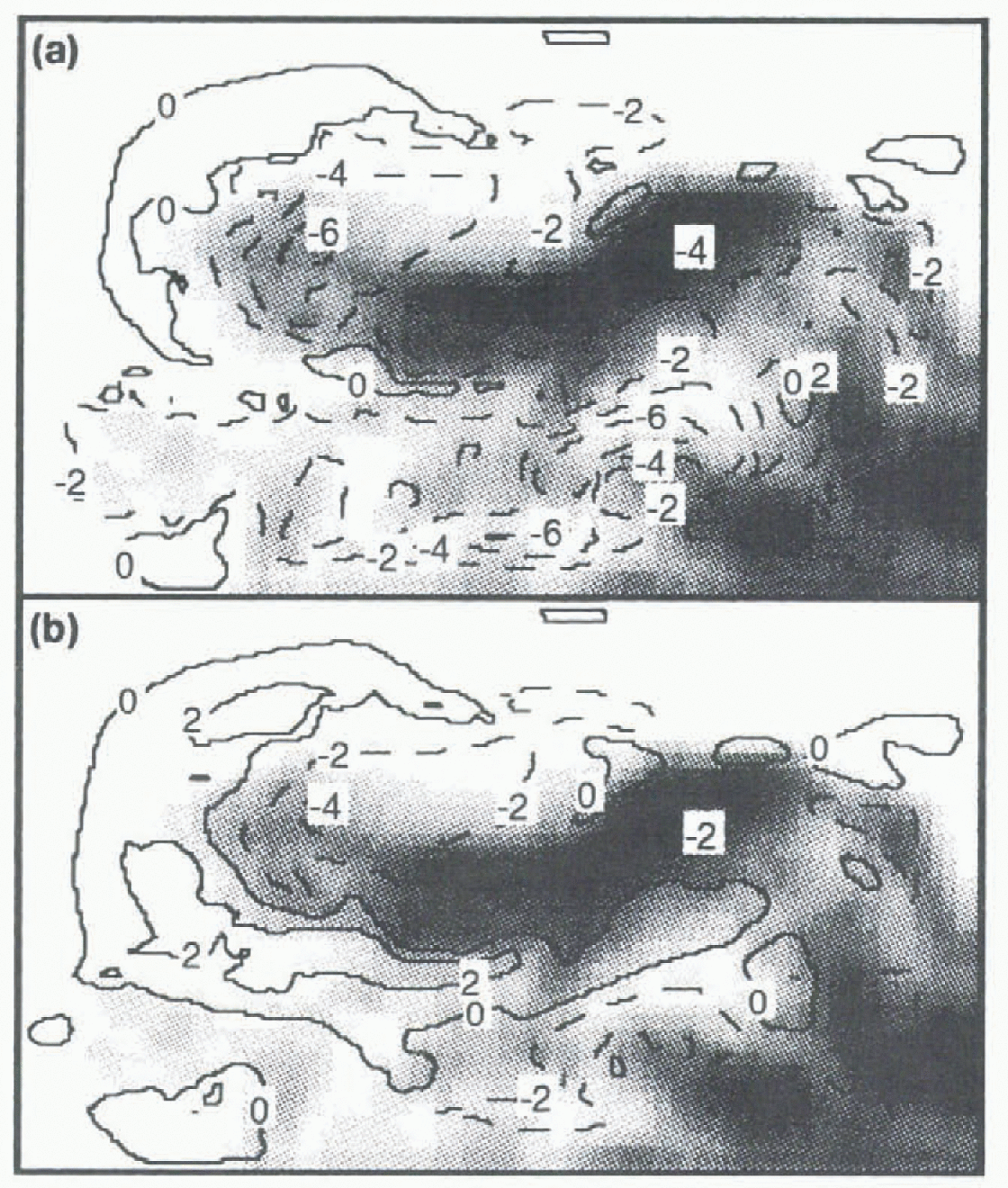
Fig. 2. Surface-air temperature biases for the (a) BATS and (b) LSM simulations compared to ECMWF analyses in degrees K.

While examining such biases can be a good guide as to the general performance of the model, it is a limited and univariate approach, Because ofthe large amounts of output available from any model simulation, it is advantageous to use a data-reduction technique, such as PCA, to view the data in a multivariate and time-varying space. The results of such an analysis of the BATS and LSM realizations, together with the LCMWF analyses for comparison, are shown in Figure 3.

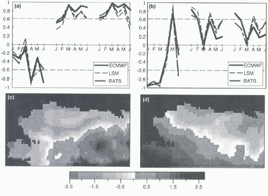
Fig. 3. Component loading patterns for (a) eigenvector 1 (“summer/continental” pattern) and (b) eigenvector 2 (“winter/maritime” pattern); from left to right. The patterns prepresent SLP, SFT and SFQ. The corresponding component scores from the LSM simulation are (c) eigenvector 1 and (d) eigenvector 2.

There is no a priori method to determine the significance of PCA loadings (Fig. 3a and b). An arbitrary significance level of an absolute value greater than 0.6 is suggested. Loadings falling below this are less well-correlated with the eigenvector variance, and hence less valuable for comparison. The score values (Fig.3c and d) may be interpreted as standard deviations from a pattern mean. The greater the score value, the more that gridcell demonstrates similarity to the loading values. For example, the January SFT loading is highly positive (>0.6) and where the scores are also high : (>1.0) then those gridcells are “warm”. Similarly, the January SLP loading is strongly negative i (<-0.6), and positive scores indicate regions of low pressure and negative scores indicate high-pressure areas.

The higher ECMWF loadings indicate a greater coherence of structure due to the lower resolution of the analyses, compared to the mesosealc structure that is possible in the ARCSyM results. The LSM and BALS loadings do not change through the spring transition as stronglv or monoto-nieally as the observational analyses. LSM, while following BATS in temperature, has a tendency in the moisture fields to exhibit more fluctuation between the summer and winter regimes. The scores associated with these loadings (representing the spatial variance) are shown in Figure 3c for the LSM simulation. The Iirsi eigenvector indeed represents a “summer/continental” pattern, primarily in temperature and moisture, with a thermal low centred over the southeastern part of the domain, associated with high temperatures and moisture in the boundary layer. This seasonal pattern shown in the loadings is interrupted somewhat in April and June, where loadings on the eigenvector drop below the 0.6 threshold; in both months, anomalous cyclone activity created a situation closer to the vvinter pattern described in eigenvector two below. This is reflected in lite concomitant rise in the eigenvector two loading values on SFT and SFQ in these months. Regardless of this anomaly, the seasonal transition beginning in March remains evident, and would most likely be enhanced with a full annual cycle where more winter months are included in the analysis.

The second eigenvector loadings demonstrate a “winter/ maritime” pattern, primarily in SLP ( Fig. 3b). Temperature also exhibits some of this winter pattern in the ARCSyM simulations, but the BATS moisture is less coherent with this pattern. Characteristic of this “winter/maritime pattern” are strong Aleutian and Bering Sea cyclonic activities combined with a zonal-temperature and moisture structure (Fig. 3d).

Major shortcomings ofthe use of ECMWF analyses to verily model ability include spatial resolution and the limited-input database, due to the operational nature of the analyses. By comparing the model realizations directly to station data, a more detailed picture of model performance can be developed. There are four stations performing regular soundings within the computational model domain. A selection of results from the Kotzebuc station (indicated in Fig. 1) is shown in Figure 4.

Figure 4a shows the temperature biases between the BATS and LSM simulations throughout the six-month period at Kotzcbue. for all vertical levels. Looking at the surface first, BATS is cooler in winter (January February), and warmer in spring and summer, with greatest warming in April a crucial transition period). The differences between the two runs extend strongly through the boundary layer and weakens to <1°C above the low-level clouds (Fig. 4b), although there is also some mid-level bias (BATS warmer) in June. While cloudiness at all levels is not systemtically greater in LSM, the low-level cloud is generally greater, and the total cloud over the column is also greater, until the month ofJune. The imparl of the increased low-level cloud in LSM changes as the shortwave radiation increases from the winter zero minimum. In winter, with less low cloud in the BATS simulation, there is greater longwave cooling, VMth no incoming shortwave radiation (not shown . Moving into spring brings greater shortwave radiation, allowing warming ofthe surface in the BATS run. but not in the LSM run where there is greater low-level cloud cover. The precipitation (Fig. 4c) i is larger in LSM in all months, with the difference increasing towards summer.

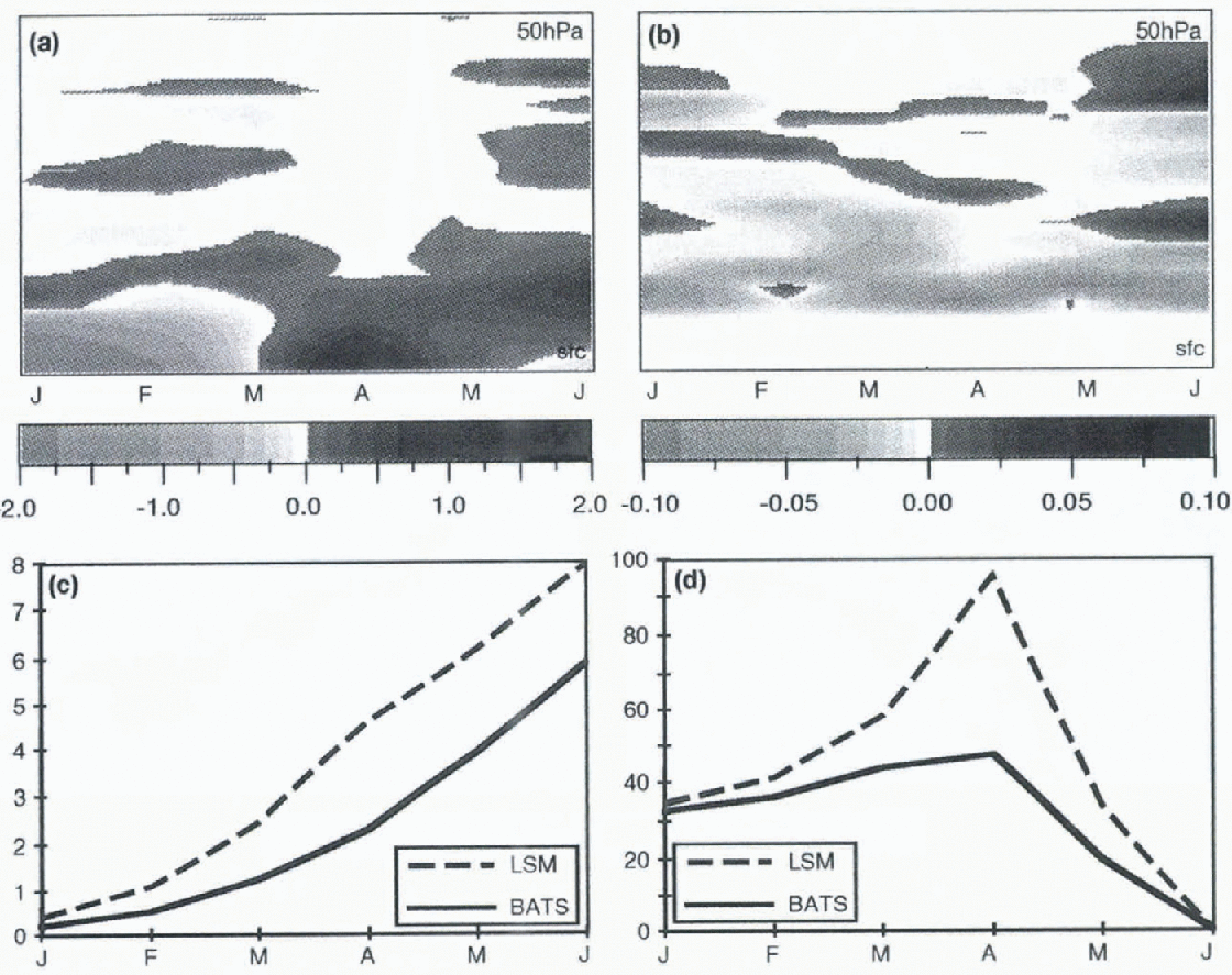
Fig. 4. Time series of BATS and LSM modelled quantities at Kotzebue: (a) air temperature differences (BATS-LSM); (b) cloud cover differences (BATS LSM); (c) precipitation and (d) snow cover.

The warmer temperatures and lower precipitation in BATS allow earlier snowmelt (Fig. 4d). Because ofthe generally drier nature of the BATS run, this is reflected in smaller moisture fluxes from the surface (not shown) — in LSM the surface latent heat flux is non-zero in winter, and continues to increase through spring as the BATS flux decreases.

There are two aspects of model formulation that are important here. Firstly, LSM allows Iiir greater “surface pooling” of moisture by a delayed infiltration in the upper layer. Thus, there is more available moisture in the LSM package than in the BAl S package allowing greater latent heat fluxes from the surface. Secondly, LSM includes a parameterization of snow albedo that depends on snow-grain size and has the effect that snow albedo decreases with increasing temperature. The effect of this can be seen in the more rapid rate of snowmelt in the ARCSyM-LSM simulation, which means that even with greater snow depth and lower temperatures, snow-free conditions are reached at about the same lime. This behaviour is reflected in varying degrees at the other stations (Fairbanks, Nome and Barrow), and suggests that the hydrological cycle is crucial in controlling the differences between the BATS and LSM models.

Conclusion

This study used three methods to compare the behaviour in high latitudes of two land-surface vegetation models within a regional climate model. These methods included simple comparisons of model-output fields with observational analyses, a multivariate analysis using PCA, and dired comparison with station soundings. The use ofthe multivariate PCA provided an overview ofthe seasonal cycle, showing the transition between the dominant winter and summer patterns. The PCA also guided use of station data, and can indicate how representative behaviour at a single point is over a greater region.

It was found that the representation ofthe hydrological cycle is a crucial component in the accurate simulation of the Arctic boundary layer. In particular, the interactions between the seasonal cycles of incoming shortwave radiation, boundary-layer cloudiness and snow cover are extremely important and vet to be fully characterized.

Comparisons of this sort provide a valuable measure of land-surface model performance. BATS and LSM are widely used in GCMs and can potentially produce different impacts and strong feedbacks in the boundary layer, which will vary with latitude. Thus, it is vital to characterize fully the potential biases in different regions resulting from the choice of specific model components.