


1. Introduction
Avalanches and landslides, as well as many industrial processes, can be classified as granular flows. Substantially improved rheological formulations have given rise to numerous attempts to simulate these phenomena with models of Navier–Stokes type. The vast number of studies rely on the  $\mu (I)$-rheology and its derivatives. The core of the
  $\mu (I)$-rheology is the Drucker–Prager yield criterion (Drucker & Prager Reference Drucker and Prager1952; Rauter, Barker & Fellin Reference Rauter, Barker and Fellin2020) and the recognition that the friction coefficient
  $\mu$ is solely a function of the inertial number
  $I$ (GDR MiDi 2004; Jop, Forterre & Pouliquen Reference Jop, Forterre and Pouliquen2006). Further studies found a similar correlation between the inertial number and the packing density
  $\phi$ (Forterre & Pouliquen Reference Forterre and Pouliquen2008).
A similar scaling was found in granular flows with low Stokes numbers  $St$ (see (2.31)). The Stokes number is related to the ratio between inertia and drag force on a particle and thus describes the influence of ambient fluid on the granular flow dynamics (e.g. Finlay Reference Finlay2001). Small Stokes numbers indicate a strong influence of the pore fluid on the particles, and hence also on the landslide dynamics. In this regime, the viscous number
  $J$ replaces the inertial number
  $I$ as a control parameter for the friction coefficient
  $\mu$ and the packing density
  $\phi$, forming the so-called
  $\mu (J)$,
  $\phi (J)$-rheology (Boyer, Guazzelli & Pouliquen Reference Boyer, Guazzelli and Pouliquen2011). Furthermore, excess pore pressure can be remarkably high under these conditions and it is imperative to explicitly consider it in numerical simulations. High drag forces and respectively small Stokes numbers are usually related to small particles. They are virtually omnipresent in geophysical flows: submarine landslides (Kim et al. Reference Kim, Løvholt, Issler and Forsberg2019), turbidity currents (Heerema et al. Reference Heerema2020), powder snow avalanches (Sovilla, McElwaine & Louge Reference Sovilla, McElwaine and Louge2015) and pyroclastic flows (Druitt Reference Druitt1998) can be dominated by fine-grained components. It follows that a large proportion of gravitational mass flows occur at low Stokes numbers, and a deeper understanding of the respective processes is relevant for research in many areas.
Incompressible granular flow models have been applied in different forms to various problems in the past decade. Lagrée, Staron & Popinet (Reference Lagrée, Staron and Popinet2011) were the first to conduct numerical simulations of subaerial granular collapses with the  $\mu (I)$-rheology and the finite-volume method. Staron, Lagrée & Popinet (Reference Staron, Lagrée and Popinet2012) used the same method to simulate silo outflows, and Domnik et al. (Reference Domnik, Pudasaini, Katzenbach and Miller2013) used a constant friction coefficient to simulate granular flows on inclined planes. Von Boetticher et al. (Reference von Boetticher, Turowski, McArdell, Rickenmann and Kirchner2016, Reference von Boetticher, Turowski, McArdell, Rickenmann, Hürlimann, Scheidl and Kirchner2017) applied a similar model, based on OpenFOAM, to debris flows, and many more examples can be found in the literature. More recently, compressible flow models have been introduced to simulate subaquatic granular flows at low Stokes numbers. The applied methods include, for example, smoothed particle hydrodynamics (Wang et al. Reference Wang, Wang, Peng and Meng2017), coupled lattice Boltzmann and discrete-element method (Yang, Kwok & Sobral Reference Yang, Kwok and Sobral2017), the material point method (Baumgarten & Kamrin Reference Baumgarten and Kamrin2019) or the finite-volume multiphase framework of OpenFOAM (Si, Shi & Yu Reference Si, Shi and Yu2018a). Results have often been compared to the experiments of Balmforth & Kerswell (Reference Balmforth and Kerswell2005) (subaerial) and Rondon, Pouliquen & Aussillous (Reference Rondon, Pouliquen and Aussillous2011) (subaquatic), two works that have gained benchmark character in the granular flow community.
Most of the mentioned applications rely on standard methods from computational fluid dynamics. This is reasonable, considering the similarity between the hydrodynamic (Navier–Stokes) equations and the granular flow equations. However, the pressure- dependent and shear-thinning viscosity associated with granular flows introduces considerable conceptual and numerical problems. The unconditional ill-posedness of an incompressible granular flow model with constant friction coefficient was described by Schaeffer (Reference Schaeffer1987), and the partial ill-posedness of the  $\mu (I)$-rheology by Barker et al. (Reference Barker, Schaeffer, Bohorquez and Gray2015). By carefully tuning the respective relations, Barker & Gray (Reference Barker and Gray2017) were able to regularize the
  $\mu (I)$-rheology for all but very high inertial numbers. Barker et al. (Reference Barker, Schaeffer, Shearer and Gray2017) described a well-posed compressible rheology, incorporating the
  $\mu (I)$-rheology as a special case.
Another pitfall of granular rheologies is the concept of effective pressure. When pore pressure is considerably high (i.e. at low Stokes numbers), it is imperative to distinguish between effective pressure and total pressure (first described by Terzaghi (Reference Terzaghi1925)). Effective pressure represents normal forces in the grain skeleton, which have a stabilizing effect, in contrast to pore pressure, which has no stabilizing effect. This has been shown to be a major issue, as pore pressure, and consequently the effective pressure, reacts very sensitively to the packing density and dilatancy (Rondon et al. Reference Rondon, Pouliquen and Aussillous2011).
Besides the rheology, tracking of the slide geometry poses a major challenge. Surface tracking is usually implemented in terms of the algebraic volume-of-fluid method (e.g. Lagrée et al. Reference Lagrée, Staron and Popinet2011; Si et al. Reference Si, Shi and Yu2018a), the level-set method (e.g. Savage, Babaei & Dabros Reference Savage, Babaei and Dabros2014), geometric surface tracking methods (e.g. Roenby, Bredmose & Jasak Reference Roenby, Bredmose and Jasak2016; Marić, Marschall & Bothe Reference Marić, Marschall and Bothe2018) or particle-based methods (e.g. Wang et al. Reference Wang, Wang, Peng and Meng2017; Baumgarten & Kamrin Reference Baumgarten and Kamrin2019).
The volume-of-fluid method, which is also used in this work, allows one to track the slide as a single component but also as a mixture of multiple phases (grains and pore fluid). Components are defined therein as objects (e.g. the landslide) that completely cover a bounded region in space without mixing with other components (e.g. the ambient fluid); see figure 3. The tracking becomes a purely geometric problem (see e.g. Roenby et al. (Reference Roenby, Bredmose and Jasak2016) for a geometric interpretation). In contrast, phases (e.g. grains) are dispersed and mixed with other phases (e.g. pore fluid) to represent the dynamic bulk of the landslide; see figure 1.

Figure 1. Definition of phase fractions  $\phi _i$ and phase velocities
  $\boldsymbol {u}_i$ inside and outside a dense granular avalanche for the two-phase model. Phase velocities can differ, allowing phase fractions to change, giving the avalanche compressible properties.
Componentwise tracking is used in various landslide models (e.g. Lagrée et al. Reference Lagrée, Staron and Popinet2011; Domnik et al. Reference Domnik, Pudasaini, Katzenbach and Miller2013; Barker & Gray Reference Barker and Gray2017). Components, i.e. the slide and the surrounding fluid, are immiscible and separated by a sharp interface. Usually, this also implies that the model is incompressible. Phase-wise tracking is commonly applied in chemical engineering (Gidaspow Reference Gidaspow1994; van Wachem Reference van Wachem2000; Passalacqua & Fox Reference Passalacqua and Fox2011) and has recently been introduced to environmental engineering (e.g. Chauchat et al. Reference Chauchat, Cheng, Nagel, Bonamy and Hsu2017; Cheng, Hsu & Calantoni Reference Cheng, Hsu and Calantoni2017; Si et al. Reference Si, Shi and Yu2018a). This approach allows one to describe a variable mixture of grains and pore fluid that merges smoothly into the ambient fluid. The description of the pore fluid as an individual phase enables the model to decouple effective pressure from pore pressure, which is imperative in many flow configurations, e.g. for low Stokes numbers.
In this work, a two-component Navier–Stokes type model and a two-phase Navier–Stokes type model are applied to granular flows. Both models are implemented into the open-source toolkit OpenFOAM (Weller et al. Reference Weller, Tabor, Jasak and Fureby1998; Rusche Reference Rusche2002; OpenCFD Ltd 2004), using the volume-of-fluid method for component- and phase-wise tracking (see § 2). Subaerial (Balmforth & Kerswell Reference Balmforth and Kerswell2005) and subaquatic granular collapses (Rondon et al. Reference Rondon, Pouliquen and Aussillous2011) are simulated with both models and results are compared with the respective experiments and with each other.
We apply the  $\mu (I)$,
  $\phi (I)$-rheology to subaerial cases (
 $St \gtrapprox 1$) and the
  $\mu (J)$,
  $\phi (J)$-rheology to subaquatic cases (
 $St \lessapprox 1$). The two-component model applies simplified rheologies in the form of the incompressible
  $\mu (I)$ and
  $\mu (J)$-rheologies. The
  $\phi (I)$ and
  $\phi (J)$ curves are merged into the particle pressure relation of Johnson & Jackson (Reference Johnson and Jackson1987) to achieve the correct quasi-static limits (Vescovi, di Prisco & Berzi Reference Vescovi, di Prisco and Berzi2013). This yields reasonable values for the packing density at rest, which is imperative for granular collapses with static regions. In contrast to many previous works (e.g. Savage et al. Reference Savage, Babaei and Dabros2014; von Boetticher et al. Reference von Boetticher, Turowski, McArdell, Rickenmann, Hürlimann, Scheidl and Kirchner2017; Si et al. Reference Si, Shi and Yu2018a), we renounce additional contributions to shear strength (e.g. cohesion) because we do not see any physical justification (e.g. electrostatic forces, capillary forces, cementing) in the investigated cases. We apply a very transparent and simple model, focusing on the relevant physical processes, and achieve a remarkable accuracy, especially in comparison to more complex models (e.g. Si et al. Reference Si, Shi and Yu2018a; Baumgarten & Kamrin Reference Baumgarten and Kamrin2019). Further, it is shown that various experimental set-ups with different initial packing densities can be simulated with the same constitutive parameters, whereas many previous attempts required individual parameters for different cases (e.g. Savage et al. Reference Savage, Babaei and Dabros2014; Wang et al. Reference Wang, Wang, Peng and Meng2017; Si et al. Reference Si, Shi and Yu2018a).
The paper is organized as follows. The multiphase (§ 2.1) and multicomponent (§ 2.2) models are introduced in § 2, including models for granular viscosity (§ 2.3), granular particle pressure (§§ 2.4 and 2.5) and drag (§ 2.6). Results are shown and discussed in § 3 for a subaerial case and in § 4 for two subaquatic cases. A conclusion is drawn in § 5 and a summary is given in § 6. Furthermore, a thorough sensitivity analysis is provided in the Appendix.
2. Methods
2.1. Two-phase landslide model
The two-phase model is based on the phase momentum and mass conservation equations (see e.g. Rusche Reference Rusche2002). The governing equations for the continuous fluid phase are given as
 \begin{gather} \frac{\partial \phi_{{c}}}{\partial t} + \boldsymbol{\nabla}\boldsymbol{\cdot}(\phi_{{c}} \boldsymbol{u}_{{c}}) =0, \end{gather}
 \begin{gather}\frac{\partial \phi_{{c}} \rho_{{c}} \boldsymbol{u}_{{c}}}{\partial t} + \boldsymbol{\nabla}\boldsymbol{\cdot}(\phi_{{c}} \rho_{{c}} \boldsymbol{u}_{{c}}\otimes\boldsymbol{u}_{{c}}) =\boldsymbol{\nabla}\boldsymbol{\cdot}(\phi_{{c}} {\boldsymbol{\mathsf{T}}}_{{c}})-\phi_{{c}} \boldsymbol{\nabla} p+\phi_{{c}} \rho_{{c}} \boldsymbol{g}+ k_{{gc}}(\boldsymbol{u}_{{g}}-\boldsymbol{u}_{{c}}), \end{gather}
and for the grains as
 \begin{gather} \frac{\partial \phi_{{g}}}{\partial t} + \boldsymbol{\nabla}\boldsymbol{\cdot}(\phi_{{g}} \boldsymbol{u}_{{g}}) = 0, \end{gather}
 \begin{gather}\frac{\partial \phi_{{g}} \rho_{{g}} \boldsymbol{u}_{{g}}}{\partial t} + \boldsymbol{\nabla}\boldsymbol{\cdot}(\phi_{{g}} \rho_{{g}} \boldsymbol{u}_{{g}}\otimes\boldsymbol{u}_{{g}}) =\boldsymbol{\nabla}\boldsymbol{\cdot}(\phi_{{g}} {\boldsymbol{\mathsf{T}}}_{{g}})- \boldsymbol{\nabla}\,p_{{s}}-\phi_{{g}} \boldsymbol{\nabla} p+\phi_{{g}} \rho_{{g}} \boldsymbol{g}+k_{{gc}}(\boldsymbol{u}_{{c}}-\boldsymbol{u}_{{g}}). \end{gather}
Here the phase-fraction fields  $\phi _{{g}}$ and
  $\phi _{{c}}$, i.e. the phase volume over the total volume (the index
  $i$ indicates either
  ${c}$ or
  ${g}$),
 \begin{equation} \phi_{i} = \frac{V_{i}}{V}, \end{equation}
describe the composition of the grain–fluid mixture; see figure 1. The granular phase fraction is identical to the packing density  $\phi = \phi _{{g}}$. Phase fractions take values between zero and one and the sum of all phase fractions yields one. The pore fluid is assumed to match the surrounding fluid, and the respective phase fraction
  $\phi _{{c}}$ is therefore one outside the slide. This way, phase-fraction fields provide a mechanism to track not only the packing density of the slide, but also its geometry. Every phase moves with a unique velocity field
  $\boldsymbol {u}_{i}$, which is not divergence-free. This allows the mixture to change, yielding a variable packing density and thus bulk compressibility, although the phase densities
  $\rho _{{g}}$ and
  $\rho _{{c}}$ are constant. The volume-weighted average velocity is divergence free,
 \begin{equation} \boldsymbol{\nabla}\boldsymbol{\cdot} \bar{\boldsymbol{u}} = \boldsymbol{\nabla}\boldsymbol{\cdot} (\phi_{{g}} \boldsymbol{u}_{{g}} + \phi_{{c}} \boldsymbol{u}_{{c}} ) = 0,\end{equation}
which allows one to use numerical methods for incompressible flow.
The pore pressure (or shared pressure)  $p$ acts on all phases equally, while the grain phase experiences additional pressure due to force chains between particles, the so-called effective pressure (or particle pressure)
  $p_{{s}}$; see figure 2. The effective pressure is a function of the packing density in this model, and the balance between effective pressure and external pressure (e.g. overburden pressure) ensures realistic packing densities. The total pressure can be assembled as
 \begin{equation} p_{{tot}} = p + p_{{s}}.\end{equation}
Figure 2. Representative volume element of a grain–fluid mixture. The effective pressure  $p_{{s}}$ (red arrows) represents normal forces in the grain skeleton (black arrows). The pore pressure (blue arrows) represents pressure that is equally shared by pore fluid and grains.
The deviatoric phase stress tensors are expressed as
 \begin{equation} {\boldsymbol{\mathsf{T}}}_i = 2 \rho_i \nu_i{\boldsymbol{\mathsf{S}}}_i,\end{equation}
with phase viscosity  $\nu _i$, phase density
  $\rho _i$ and deviatoric phase strain-rate tensor
 \begin{equation} {\boldsymbol{\mathsf{S}}}_i = \tfrac{1}{2}(\boldsymbol{\nabla}\boldsymbol{u}_i + (\boldsymbol{\nabla}\boldsymbol{u}_i)^\textrm{T}) - \tfrac{1}{3}\boldsymbol{\nabla} \boldsymbol{\cdot} \boldsymbol{u}_i {\boldsymbol{\mathsf{I}}}. \end{equation}
The viscosity of the pore fluid  $\nu _{{c}}$ is usually constant and the granular viscosity
  $\nu _{{g}}$ follows from constitutive models like the
  $\mu (I)$-rheology (see § 2.3). The total deviatoric stress tensor can be calculated as
 \begin{equation} {\boldsymbol{\mathsf{T}}} = \phi_{{c}} {\boldsymbol{\mathsf{T}}}_{{c}} + \phi_{{g}} {\boldsymbol{\mathsf{T}}}_{{g}}.\end{equation}
 The last terms in (2.2) and (2.4) represent drag forces between phases and  $k_{{gc}}$ is the drag coefficient of the grains in the pore fluid. Lift and virtual mass forces are neglected in this work, because they play a minor role (Si et al. Reference Si, Shi and Yu2018a).
The granular viscosity  $\nu _{{g}}$, the effective pressure
  $p_{{s}}$ and the drag coefficient
  $k_{{gc}}$ represent interfaces to exchangeable submodels, presented in §§ 2.3–2.6.
2.2. Two-component landslide model
Many two-phase systems can be substantially simplified by assuming that phases move together, i.e. that phase velocities are equal,
 \begin{equation} \boldsymbol{u}_{i} \approx \bar{\boldsymbol{u}} = \phi_{{g}} \boldsymbol{u}_{{g}} + \phi_{{c}} \boldsymbol{u}_{{c}}.\end{equation}
This fits very well to completely separated phases that are divided by a sharp interface (e.g. surface waves in water Rauter et al. (Reference Rauter, Hoße, Mulligan, Take and Løvholt2021)), but also systems of mixed phases (e.g. grains and fluid) can be handled to some extent (e.g. Lagrée et al. Reference Lagrée, Staron and Popinet2011). The phase momentum conservation equations (2.2) and (2.4) can be combined into a single momentum conservation equation and the system takes the form of the ordinary Navier–Stokes equations with variable fluid properties (see e.g. Rusche Reference Rusche2002),
 \begin{gather} \frac{\partial \rho\bar{\boldsymbol{u}}}{\partial t} + \boldsymbol{\nabla}\boldsymbol{\cdot}(\rho\bar{\boldsymbol{u}}\otimes\bar{\boldsymbol{u}}) = \boldsymbol{\nabla}\boldsymbol{\cdot}{\boldsymbol{\mathsf{T}}}-\boldsymbol{\nabla}\,p_{{tot}}+\rho \boldsymbol{g}, \end{gather}
 \begin{gather}\boldsymbol{\nabla}\boldsymbol{\cdot}\bar{\boldsymbol{u}} = 0. \end{gather}
A detailed derivation can be found in Appendix A. The pressure is denoted as  $p_{{tot}}$, indicating that it contains contributions from hydrodynamic and effective pressure.
The phase-fraction fields  $\phi _i$ cannot be recovered after this simplification and the method switches to the tracking of components instead of phases; see figure 3. Components are tracked with so-called component indicator functions
  $\alpha _i$ (sometimes called phase indicator functions but herein we distinguish phases from components), being either one if component
  $i$ is present at the respective location or zero otherwise,
 \begin{equation} \alpha_i = \begin{cases} 1 & \text{if component}\ i\ \text{is present,}\\ 0 & \text{otherwise.} \end{cases} \end{equation}
Values between zero and one are not intended by this method and only appear due to numerical reasons, i.e. the discretization of the discontinuous field (see § 2.7). Herein, two component indicator functions are used, one for the ambient fluid component,  $\alpha _{{c}}$, and one for the slide component,
  $\alpha _{{s}}$ (see figure 3). Evolution equations for component indicator functions can be derived from mass conservation equations as
 \begin{equation} \frac{\partial \alpha_i}{\partial t} + \boldsymbol{\nabla}\boldsymbol{\cdot}(\alpha_i\bar{\boldsymbol{u}}) = 0.\end{equation}
Figure 3. Definition of component indicator functions  $\alpha _i$ and the velocity
  $\bar {\boldsymbol {u}}$ inside and outside a dense granular avalanche for the two-component model.
The definition of components is straightforward for completely separated phases, where components can be matched with phases, e.g. water and air. The definition of the slide component, on the other hand, is not unambiguous, as it consists of a variable mixture of grains and pore fluid. A boundary of the slide component can, for example, be found by defining a limit for the packing density (e.g. 50 % of the average packing density). Further, a constant reference packing density  $\bar {\phi }$ has to be determined, which is assigned to the whole slide component. The density of the slide component follows as
 \begin{equation} \rho_{{s}} = \bar{\phi}\rho_{{g}} + (1-\bar{\phi})\rho_{{c}},\end{equation}
and a similar relation can be established for the deviatoric stress tensor (see § 2.3.1).
The local density  $\rho$ and the local deviatoric stress tensor
  ${\boldsymbol{\mathsf{T}}}$ can be calculated as
 \begin{gather} \rho = \sum_i \alpha_i \rho_i = \alpha_{{s}} \rho_{{s}} + \alpha_{{c}} \rho_{{c}}, \end{gather}
 \begin{gather}{\boldsymbol{\mathsf{T}}} = \sum_i \alpha_i {\boldsymbol{\mathsf{T}}}_i =\alpha_{{s}} {\boldsymbol{\mathsf{T}}}_{{s}} + \alpha_{{c}} {\boldsymbol{\mathsf{T}}}_{{c}}, \end{gather}
using component densities  $\rho _{i}$, as well as component deviatoric stress tensors
  ${\boldsymbol{\mathsf{T}}}_{i}$. Component deviatoric stress tensors are calculated as
 \begin{equation} {\boldsymbol{\mathsf{T}}}_{i} = 2\rho_i \nu_i {\boldsymbol{\mathsf{S}}}, \end{equation}
with the component viscosity  $\nu _i$ and the deviatoric shear-rate tensor
  ${\boldsymbol{\mathsf{S}}}$. Note that the deviatoric shear-rate tensor
  ${\boldsymbol{\mathsf{S}}}$ matches the shear-rate tensor
  ${\boldsymbol{\mathsf{D}}}$, because the volume-weighted averaged velocity field is divergence-free,
 \begin{equation} {\boldsymbol{\mathsf{S}}} = {\boldsymbol{\mathsf{D}}} = \tfrac{1}{2}(\boldsymbol{\nabla} \bar{\boldsymbol{u}}+(\boldsymbol{\nabla} \bar{\boldsymbol{u}})^\textrm{T}). \end{equation}
The viscosity of the ambient fluid  $\nu _{{c}}$ is usually constant and the viscosity of the slide region
  $\nu _{{s}}$ follows from granular rheology; see § 2.3.
2.3. Rheology
2.3.1. Unifying rheologies
Most granular rheologies (e.g. the  $\mu (I)$-rheology) are defined in terms of the total deviatoric stress tensor in the slide component
  ${\boldsymbol{\mathsf{T}}}_{{s}}$. This has to be accounted for and corrected in the two-phase model if the same viscosity model is used in both models. Similar to (2.16), component viscosities can be related to phase viscosities as
 \begin{gather} {\boldsymbol{\mathsf{T}}}_{{s}} = \bar{\phi}{\boldsymbol{\mathsf{T}}}_{{g}} + (1-\bar{\phi}) {\boldsymbol{\mathsf{T}}}_{{c}}, \end{gather}
 \begin{gather}2 \rho_{{s}} \nu_{{s}}{\boldsymbol{\mathsf{S}}}_{{s}} = 2\bar{\phi}\rho_{{g}} \nu_{{g}} {\boldsymbol{\mathsf{S}}}_{{g}} + 2(1-\bar{\phi})\rho_{{c}} \nu_{{c}} {\boldsymbol{\mathsf{S}}}_{{c}}. \end{gather}
The contribution of the granular phase to stresses is assumed to be much higher than the contribution of the pore fluid,  $\bar {\phi }\rho _{{g}} \nu _{{g}} {\boldsymbol{\mathsf{S}}}_{{g}} \gg (1-\bar {\phi })\rho _{{c}} \nu _{{c}} {\boldsymbol{\mathsf{S}}}_{{c}}$. Further, by neglecting the mass of the pore fluid,
  $\rho _{{s}} \approx \bar {\phi } \rho _{{g}}$, it follows that kinematic viscosities have to be similar in both models,
 \begin{equation} \nu_{{s}} \approx \nu_{{g}}. \end{equation}
Alternatively, one can match the dynamic viscosities  $\nu _{{s}} \rho _{{s}}$ and
  $\nu _{{g}} \rho _{{g}}$ if the factor
  $\phi _{{g}}$ is removed from the viscous term in (2.4). Note that these assumptions are fairly accurate for subaerial granular flows but questionable for subaquatic granular flows. However, multiphase and multicomponent models differ substantially under subaquatic conditions and a unification is not possible.
2.3.2. Drucker–Prager plasticity model
An important characteristic of granular materials is the pressure-dependent shear stress, described by the Drucker–Prager yield criterion (Drucker & Prager Reference Drucker and Prager1952). Schaeffer (Reference Schaeffer1987) was the first to include granular friction in the Navier–Stokes equations by expressing the Drucker–Prager yield criterion in terms of the shear-rate tensor and the pressure,
 \begin{equation} {\boldsymbol{\mathsf{T}}}_{{s}} = \mu p_{{s}}\frac{{\boldsymbol{\mathsf{S}}}}{\|{\boldsymbol{\mathsf{S}}}\|},\end{equation}
where the norm of a tensor  $\|{\boldsymbol{\mathsf{A}}}\|$ is defined as
 \begin{equation} \|{\boldsymbol{\mathsf{A}}}\| = \sqrt{\tfrac{1}{2} \,\textrm{tr}({\boldsymbol{\mathsf{A}}}^2)}.\end{equation}
The friction coefficient  $\mu$ is constant and a material parameter in the first model by Schaeffer (Reference Schaeffer1987). The slide component viscosity follows as
 \begin{equation} \nu_s = |T_s|/(2\rho_s |S|) = \mu p_s/(2\rho_s |S|).\end{equation}
This relation has been applied with slight modifications by, for example, Domnik et al. (Reference Domnik, Pudasaini, Katzenbach and Miller2013), Savage et al. (Reference Savage, Babaei and Dabros2014) and Rauter et al. (Reference Rauter, Barker and Fellin2020). Following the findings in § 2.3.1, the kinematic viscosity of slide and grains have to be similar and the granular phase viscosity follows as
 \begin{equation} \nu_s = |T_g| / (2 \rho_s |S_g|) = \mu p_s / ( 2 \rho_g \phi |S_g|).\end{equation}
The viscosity reaches very high values for  $\|{\boldsymbol{\mathsf{S}}}\| \rightarrow 0$ and very small values for
  $p_{{s}} \rightarrow 0$, and both limits can lead to numerical problems.
To overcome numerically unstable behaviour, the viscosity is truncated to an interval  $[\nu _{min}, \nu _{max}]$. A thoughtful choice of
  $\nu _{max}$ is crucial for the presented method. Small values tend towards unphysical results, because solid-like behaviour can only be simulated by very high viscosities. Large values, on the other hand, tend towards numerical instabilities (see § 2.7.3). The ideal value for the maximum viscosity depends on the respective case and can be estimated with a scaling and sensitivity analysis (see Appendix B.1). The relation
 \begin{equation} \nu_{{max}} = \tfrac{1}{10} \sqrt{|\boldsymbol{g}| H^3},\end{equation}
where  $H$ is the characteristic height of the investigated case, was found to give a good estimate for a reasonable viscosity cutoff. Notably, the Drucker–Prager yield surface leads to an ill-posed model (Schaeffer Reference Schaeffer1987) and the truncation of the viscosity is not sufficient for a regularization. Schaeffer (Reference Schaeffer1987) did not distinguish between effective pressure and total pressure in (2.26), limiting the applications of his model substantially. We will explicitly consider effective pressure in (2.26) and (2.27) using (2.34) or (2.36) in the two-component model and (2.37), (2.40) or (2.43) in the two-phase model to avoid such limitations.
2.3.3. The  $\mu (I)$-rheology

The  $\mu (I)$-rheology (GDR MiDi 2004; Jop et al. Reference Jop, Forterre and Pouliquen2006; Forterre & Pouliquen Reference Forterre and Pouliquen2008) states that the friction coefficient
  $\mu$ is not constant in dense, dry, granular flows but rather a function of the inertial number
  $I$. The inertial number
  $I$ is defined as the ratio between the typical time scale for microscopic rearrangements of grains with diameter
  $d$, i.e.
  $t_{{micro}} = d \sqrt {\rho _{{g}}/p_{{s}}}$, and the macroscopic time scale of the deformation, i.e.
 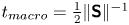 $t_{{macro}} = \tfrac {1}{2} \|{\boldsymbol{\mathsf{S}}}\|^{-1}$, thus
 \begin{equation} I = 2d \|{\boldsymbol{\mathsf{S}}}\| \sqrt{\frac{\rho_{{g}}}{p_{{s}}}}. \end{equation}
 In the two-phase model, the shear rate  ${\boldsymbol{\mathsf{S}}}$ is replaced by the deviatoric shear rate of grains
  ${\boldsymbol{\mathsf{S}}}_{{g}}$. Various approaches have been proposed for the
  $\mu (I)$ curve. Herein we apply the classic relation, given as
 \begin{equation} \mu(I) = \mu_{{1}} + (\mu_{{2}}-\mu_{{1}})\frac{I}{I_0+I},\end{equation}
where  $\mu _{{1}}$,
  $\mu _{{2}}$ and
  $I_0$ are material parameters (Jop et al. Reference Jop, Forterre and Pouliquen2006). The dynamic friction coefficient
  $\mu (I)$ is introduced into the Drucker–Prager yield criterion, (2.26) or (2.27), to get the respective granular viscosity.
2.3.4. The $\mu (J)$-rheology

At small Stokes numbers, defined as
 \begin{equation} St = 2 d^2 \|{\boldsymbol{\mathsf{S}}}\|\frac{\rho_{{g}}}{\nu_{{c}} \rho_{{c}}},\end{equation}
the pore fluid has substantial influence on the rheology and the microscopic time scale is defined by the viscous scaling 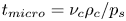 $t_{{micro}} = \nu _{{c}} \rho _{{c}}/p_{{s}}$ (Boyer et al. Reference Boyer, Guazzelli and Pouliquen2011). The friction coefficient is thus no longer a function of the inertial number
  $I$ but rather one of the viscous number
  $J$, defined as
 \begin{equation} J = 2 \|{\boldsymbol{\mathsf{S}}}\|\frac{\nu_{{c}} \rho_{{c}}}{p_{{s}}}. \end{equation}
The functional relation of the friction coefficient on the viscous number was described by Boyer et al. (Reference Boyer, Guazzelli and Pouliquen2011) as
 \begin{equation} \mu(J) = \mu_{{1}} + (\mu_{{2}}-\mu_{{1}})\frac{J}{J_0+J} + J + \frac{5}{2} \phi_{{m}} \sqrt{J},\end{equation}
where  $\mu _{{1}}$,
  $\mu _{{2}}$,
  $J_0$ and
  $\phi _{{m}}$ are material parameters (Boyer et al. Reference Boyer, Guazzelli and Pouliquen2011). The
  $\mu (J)$-rheology takes advantage of the Drucker–Prager yield criterion, similar to the
  $\mu (I)$-rheology.
Notably, the  $\mu (I)$ and
  $\mu (J)$-rheology can be combined by forming a new dimensionless number
 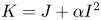 $K = J + \alpha I^2$ with a constitutive parameter
  $\alpha$ (Trulsson, Andreotti & Claudin Reference Trulsson, Andreotti and Claudin2012; Baumgarten & Kamrin Reference Baumgarten and Kamrin2019). However, this was not required for the cases presented in this work.
2.4. Effective pressure in the two-component model
2.4.1. Total pressure assumption
The two-component model is limited in considering pore pressure and dilatancy effects because the packing density is not described by this model. The effective pressure can only be reconstructed from total pressure  $p_{{tot}}$ and various assumptions. The simplest model assumes that the pore pressure is negligibly small, leading to
 \begin{equation} p_{{s}} \approx p_{{tot}}.\end{equation}
This assumption is reasonable for subaerial granular flows and has been applied to such by Lagrée et al. (Reference Lagrée, Staron and Popinet2011) and Savage et al. (Reference Savage, Babaei and Dabros2014), for example.
2.4.2. Hydrostatic pressure assumption
In subaquatic granular flows, the surrounding high-density fluid increases the total pressure substantially and it cannot be neglected. Following Savage et al. (Reference Savage, Babaei and Dabros2014), improvement can be achieved by calculating the hydrostatic pore pressure as
 \begin{equation} p_{{hs}} = \begin{cases} \rho_{{c}} \boldsymbol{g}\boldsymbol{\cdot}(\boldsymbol{x} - \boldsymbol{x_0}) & \text{for} \ \boldsymbol{g}\boldsymbol{\cdot}(\boldsymbol{x} - \boldsymbol{x_0}) > 0,\\ 0 & \text{otherwise}, \end{cases} \end{equation}
and subtracting it from the total pressure,
 \begin{equation} p_{{s}} \approx p_{{tot}} - p_{{hs}}.\end{equation}
Here,  $\boldsymbol {x}_0$ is the position of the free water surface, where the total pressure is assumed to be zero. For a variable and non-horizontal free water surface, common in landslide tsunamis, for example, this concept is complicated substantially, and, to the author's knowledge, has not been applied. Furthermore, excess pore pressure, which is common in low-Stokes-number flows, is out of the scope for this model.
2.5. Effective pressure in the two-phase model
2.5.1. Critical state theory
The structure of the two-phase model allows us to include the packing density in the effective pressure equation. Critical state theory (Roscoe, Schofield & Wroth Reference Roscoe, Schofield and Wroth1958; Schofield & Wroth Reference Schofield and Wroth1968; Roscoe Reference Roscoe1970) was the first model to describe the relationship between the effective pressure and the packing density. The critical state is defined as a state of constant packing density and constant shear stress, which is reached after a certain amount of shearing of an initially dense or loose sample. The packing density in this state, called the critical packing density  $\phi _{{crit}}$, is a function of the effective pressure
  $p_{{s}}$. This function can be inverted to get the effective pressure as a function of the critical packing density. It is further assumed that the flow is in its critical state
  $\phi _{{g}} = \phi _{{crit}}$ to obtain a model that is compatible with the governing equations. This assumption is reasonable for avalanches, slides and other granular flows but questionable for the initial release and deposition. At small deformations, the packing density might be lower (underconsolidated) or higher (overconsolidated) than the critical packing density, and the effective pressure model will over- or underestimate the effective pressure.
A popular relation for the effective pressure (the so-called critical state line) has been described by Johnson & Jackson (Reference Johnson and Jackson1987) and Johnson, Nott & Jackson (Reference Johnson, Nott and Jackson1990) as
 \begin{equation} p_{{s}} = a\frac{\phi_{{g}}-\phi_{{rlp}}}{\phi_{{rcp}}-\phi_{{g}}},\end{equation}
where  $\phi _{{rlp}}$ is the random loose packing density in the critical state,
  $\phi _{{rcp}}$ is the random close packing density in the critical state and
  $a$ is a scaling parameter. The scaling parameter
  $a$ can be interpreted as the effective pressure at the packing density
 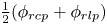 $\frac {1}{2}(\phi _{{rcp}}+\phi _{{rlp}})$. Note that we apply a simplified version of the original relation, similar to Vescovi et al. (Reference Vescovi, di Prisco and Berzi2013). Packing densities above
  $\phi _{{rcp}}$ are not valid and avoided by the asymptote of the effective pressure at
  $\phi _{{rcp}}$. If packing densities higher than or equal to
  $\phi _{{rcp}}$ appear in simulations, they should be terminated and restarted with refined numerical parameters (e.g. time-step duration).
2.5.2. The $\phi (I)$ relation

Equation (2.37) is known to hold for slow deformations in the critical state (see e.g. Vescovi et al. Reference Vescovi, di Prisco and Berzi2013). However, this relation is not consistent with granular flow experiments. Granular flows show dilatancy with increasing shear rate, expressed by Forterre & Pouliquen (Reference Forterre and Pouliquen2008), for example, as a function of the inertial number  $I$,
$I$,
 \begin{equation} \phi_{{g}}(I) = \phi_{max} -{\rm \Delta}\phi I, \end{equation}
where  $\phi _{max}$ and
  ${\rm \Delta} \phi$ are material parameters. This relation can be transformed into a model for the effective pressure by introducing the inertial number
  $I$,
$I$,
 \begin{equation} p_{{s}} = \rho_{{s}} \left(2 \|{\boldsymbol{\mathsf{S}}}_{{g}}\| d\frac{{\rm \Delta}\phi}{\phi_{max}-\phi_{{g}}}\right)^{2}.\end{equation}
 This relation has two substantial problems: (i) for  $\|{\boldsymbol{\mathsf{S}}}_{{g}}\| = 0$ it yields
  $p_{{s}} = 0$, and (ii) for
  $\phi _{{g}} = 0$ it yields
  $p_{{s}} \neq 0$, which causes numerical problems and unrealistic results. The first problem is addressed by superposing (2.39) with the quasi-static relation (2.37), similar to Vescovi et al. (Reference Vescovi, di Prisco and Berzi2013). The second problem is solved by multiplying (2.39) with the normalized packing density
  $\phi _{{g}}/\bar {\phi }$, which ensures that the pressure vanishes for
  $\phi _{{g}} = 0$. The normalization with the reference packing density
  $\bar {\phi }$ ensures that parameters (
 $\phi _{max}, {\rm \Delta} \phi$) will be similar to the original equation.
Further, to reduce the number of material parameters, we set the maximum packing density in the  $\phi (I)$ relation equal to the random close packing density
  $\phi _{{rcp}}$. The final relation reads
 \begin{equation} p_{{s}} = a\frac{\phi_{{g}}-\phi_{{rlp}}}{\phi_{{rcp}}-\phi_{{g}}} + \rho_{{g}}\frac{\phi_{{g}}}{\bar{\phi}}\left(2 \|{\boldsymbol{\mathsf{S}}}_{{g}}\| d\frac{{\rm \Delta}\phi}{\phi_{{rcp}}-\phi_{{g}}}\right)^{2},\end{equation}
and is shown in figure 4 alongside the original relations of Johnson & Jackson (Reference Johnson and Jackson1987) and Forterre & Pouliquen (Reference Forterre and Pouliquen2008). Interestingly, this relation contains many features of the extended kinetic theory of Vescovi et al. (Reference Vescovi, di Prisco and Berzi2013); compare figure 4(b) herein with figure 6(b) in Vescovi et al. (Reference Vescovi, di Prisco and Berzi2013). Notably, the inertial number is a function of only the packing density and the shear rate,  $I = f(\phi _{{g}}, \|{\boldsymbol{\mathsf{S}}}_{{g}}\|)$, because the effective pressure is calculated as a function of the packing density. The same follows for the friction coefficient,
  $\mu = f(\phi _{{g}}, \|{\boldsymbol{\mathsf{S}}}_{{g}}\|)$, and the deviatoric stress tensor,
  $\|{\boldsymbol{\mathsf{T}}}_{{g}}\| = f(\phi _{{g}}, \|{\boldsymbol{\mathsf{S}}}_{{g}}\|)$. This highlights that the two-phase model implements a density-dependent rheology, rather than a pressure-dependent rheology.

Figure 4. (a) Effective pressure  $p_{{s}}$ following the
  $\phi (I)$ relation as a function of packing density
  $\phi _{{g}}$ and deviatoric shear rate
  $\|{\boldsymbol{\mathsf{S}}}_{{g}}\|$. The dashed lines show the original relation of Forterre & Pouliquen (Reference Forterre and Pouliquen2008), the continuous coloured lines show the modified relation and the black line shows the quasi-static limit following Johnson & Jackson (Reference Johnson and Jackson1987). (b) The critical packing density as a function of particle pressure
  $p_{{s}}$ and deviatoric shear rate
  $\|{\boldsymbol{\mathsf{S}}}_{{g}}\|$. The dashed lines follow the original
  $\phi (I)$ relation, and the continuous lines show the modified version. The critical state theory would result in horizontal lines in this plot.
It should be noted that there are various possibilities to combine critical state theory and the  $\mu (I)$,
  $\phi (I)$-rheology. An alternative approach including bulk viscosity is provided, for example, by Schaeffer et al. (Reference Schaeffer, Barker, Tsuji, Gremaud, Shearer and Gray2019).
2.5.3. The $\phi (J)$ relation

The low-Stokes-number regime requires the replacement of the inertial number  $I$ with the viscous number
  $J$. The dependence of the packing density on the viscous number was described by Boyer et al. (Reference Boyer, Guazzelli and Pouliquen2011) as
 \begin{equation} \phi_{{g}} = \frac{\phi_{{m}}}{1+\sqrt{J}}, \end{equation}
and we can derive the effective pressure by inserting the viscous number as
 \begin{equation} p_{{s}} = \frac{2 \nu_{{c}} \rho_{{c}} \|{\boldsymbol{\mathsf{S}}}_{{g}}\|}{\left(\dfrac{\phi_{{m}}}{\phi_{{g}}}-1\right)^2}. \end{equation}
Notably, Boyer et al. (Reference Boyer, Guazzelli and Pouliquen2011) emphasized that  $\phi _{{m}}$ does not match the random close packing density
  $\phi _{{rcp}} \approx 0.63$ but rather is a value close to
  $0.585$. This leads to substantial problems for large values of
  $\phi _{{g}}$, as the relation is only valid for
  $\phi _{{g}} < \phi _{{m}} = 0.585$ or
  $\|{\boldsymbol{\mathsf{S}}}_{{g}}\| = 0$. In other words, shearing is only possible for
  $\phi _{{g}} < \phi _{{m}}$.
We solve this issue by allowing a creeping shear rate of  $S_0$ at packing densities above
  $\phi _{{m}}$. Further, and as before, we superpose the relation with the quasi-static relation of Johnson & Jackson (Reference Johnson and Jackson1987) to yield the correct asymptotic values for
  $\|{\boldsymbol{\mathsf{S}}}_{{g}}\| \rightarrow 0$ known from critical state theory. The final relation reads
 \begin{equation} p_{{s}} = a\frac{\phi_{{g}}-\phi_{{rlp}}}{\phi_{{rcp}}-\phi_{{g}}} + \frac{2 \nu_{{c}} \rho_{{c}} \|{\boldsymbol{\mathsf{S}}}_{{g}}\|}{\left(\dfrac{\hat{\phi}_{{m}}}{\phi_{{g}}}-1\right)^2}, \end{equation}
with
 \begin{equation} \hat{\phi}_{{m}} = \begin{cases} \phi_{{m}}+(\phi_{{rcp}}-\phi_{{m}}) (S_{0}-\|{\boldsymbol{\mathsf{S}}}\|) & \text{for} \ S_{0} > \|{\boldsymbol{\mathsf{S}}}\|, \\ \phi_{{m}} & \text{otherwise}. \end{cases} \end{equation}
The respective relation is shown in figure 5 alongside the original relations of Johnson & Jackson (Reference Johnson and Jackson1987) and Boyer et al. (Reference Boyer, Guazzelli and Pouliquen2011). States with  $\|{\boldsymbol{\mathsf{S}}}\| \geq S_0$ and
  $\phi _{{g}} \geq \phi _{{m}}$ or
  $\phi _{{g}} \geq \phi _{{rcp}}$ are not intended by this model, and simulations should be terminated if such states appear.

Figure 5. (a) Particle pressure  $p_{{s}}$ following the
  $\phi (J)$ relation as a function of packing density
  $\phi _{{g}}$ and deviatoric shear rate
  $\|{\boldsymbol{\mathsf{S}}}_{{g}}\|$. The dashed lines show the original relation of Boyer et al. (Reference Boyer, Guazzelli and Pouliquen2011), the continuous coloured lines show the modified relation and the black line shows the static limit expressed following Johnson & Jackson (Reference Johnson and Jackson1987). (b) The critical packing density as a function of particle pressure
  $p_{{s}}$ and deviatoric shear rate
  $\|{\boldsymbol{\mathsf{S}}}_{{g}}\|$. The dashed lines follow the original
  $\phi (J)$ relation, and the continuous lines show the modified version. The grey area shows the region where only creeping shear rates below
  $S_0$ are allowed.
2.6. Drag and permeability model
The drag model describes the momentum exchange between grains and pore fluid in the two-phase model and widely controls permeability, excess pore pressure relaxation and the settling velocity of grains. A wide range of drag models for various situations can be found in the literature. Herein we stick to the Kozeny–Carman relation as applied by Pailha & Pouliquen (Reference Pailha and Pouliquen2009),
 \begin{equation} k_{{g} \textrm{c}} = 150\frac{\phi_{{g}}^2 \nu_{{c}} \rho_{{c}}}{\phi_{{c}} d^2},\end{equation}
with the grain diameter  $d$ as the only parameter. This relation is assumed to be valid for small relative velocities and densely packed granular material. It has been modified to account for higher relative velocities (Ergun Reference Ergun1952) and lower packing densities (Gidaspow Reference Gidaspow1994); however, these are not relevant for the investigated configurations (see Si et al. (Reference Si, Shi and Yu2018a) for an application of the extended relation). This relation is visualized in figure 6(a) for various diameters and packing densities.

Figure 6. Drag coefficient  $k_{{gc}}$ (a) and permeability
  $\kappa$ (b) following the Kozeny–Carman relation (Pailha & Pouliquen Reference Pailha and Pouliquen2009) for various grain diameters (colour) and packing densities (
 $x$-axis).
The drag coefficient can be reformulated into a permeability coefficient as known in soil mechanics and porous media. Comparing Darcy's law (e.g. Bear Reference Bear1972) with the equations of motion for the fluid phase, we can calculate the hydraulic conductivity as
 \begin{equation} K = \frac{\rho_{{c}}|\boldsymbol{g}|}{k_{{gc}}}, \end{equation}
and furthermore the intrinsic permeability (e.g. Bear Reference Bear1972) as
 \begin{equation} \kappa = K\frac{\nu_{{c}}}{|\boldsymbol{g}|} = \frac{\nu_{{c}} \rho_{{c}}}{k_{{gc}}} = \frac{\phi_{{c}} d^2}{150 \phi_{{g}}^2}.\end{equation}
The permeability is visualized in figure 6(b). In a similar manner, the drag coefficient can be calculated as
 \begin{equation} k_{{g} \textrm{c}} = \frac{\rho_{{c}} \nu_{{c}}}{\kappa}, \end{equation}
if the intrinsic permeability of the granular material is known.
2.7. Numerical solution and exception handling
All models are implemented into OpenFOAM v1812 (Weller et al. Reference Weller, Tabor, Jasak and Fureby1998; OpenCFD Ltd 2004) and solved with the finite-volume method (Jasak Reference Jasak1996; Rusche Reference Rusche2002; Moukalled, Mangani & Darwish Reference Moukalled, Mangani and Darwish2016).
2.7.1. Two-component landslide model
The two-component model is based on the solver ‘multiphaseInterFoam’, using the PISO (pressure-implicit with splitting of operators) algorithm (Issa Reference Issa1986) and interpolations following Rhie & Chow (Reference Rhie and Chow1983) to solve the coupled system of pressure and velocity. First, an updated velocity field is calculated without the contribution of pressure. The predicted velocity field is later corrected to be divergence-free and the pressure follows from the required correction. Finally, all other fields, e.g. the phase indicator functions, are updated. This procedure is repeated in each time step.
Components (slide and ambient air or water) are divided by an interface, which is assumed to be sharp. However, the interface is often smeared by numerical diffusion. To keep the interface between components sharp, the relative velocity between phases  $\boldsymbol {u}_{{ij}}$, which was previously eliminated from the system, is reintroduced in (2.15),
 \begin{equation} \frac{\partial \alpha_i}{\partial t} + \boldsymbol{\nabla}\boldsymbol{\cdot}(\alpha_i \bar{\boldsymbol{u}}) + \boldsymbol{\nabla}\boldsymbol{\cdot}(\alpha_i \alpha_j \boldsymbol{u}_{ij}) = 0.\end{equation}
Equation (2.49) is finally solved using the MULES (multidimensional universal limiter with explicit solution) algorithm (Weller Reference Weller2008). This scheme limits the interface compression term (i.e. the term containing  $\boldsymbol {u}_{ij}$) to avoid overshoots (
 $\alpha _i > 1$) and undershoots (
 $\alpha _i < 0$) of the component indicator fields.
There is no conservation equation for the relative velocity in the two-component model and it has to be reconstructed from assumptions. Two methods are known to construct the relative velocity for granular flows. Barker et al. (Reference Barker, Rauter, Maguire, Johnson and Gray2021) suggest constructing the relative velocity for granular flows from physical effects such as segregation and settling. The relative velocity follows as the terminal velocity of spheres in the surrounding fluid under the influence of gravity. Alternatively, one can construct a velocity field that is normal to the interface and of the same magnitude as the average velocity  $\bar {\boldsymbol {u}}$,
 \begin{equation} \boldsymbol{u}_{ij} = |\bar{\boldsymbol{u}}|\frac{\alpha_{j} \boldsymbol{\nabla} \alpha_{i} - \alpha_{i} \boldsymbol{\nabla} \alpha_{j}}{|\alpha_{j} \boldsymbol{\nabla} \alpha_{i} - \alpha_{i} \boldsymbol{\nabla} \alpha_{j}|}. \end{equation}
This method has a maximum sharpening effect (Weller Reference Weller2008) and is thus also applied in this work.
2.7.2. Two-phase landslide model
The two-phase model is based on the solver ‘multiphaseEulerFoam’. The system of pressure and average velocity is solved with the same concept as in the two-component solver. The velocity fields for all phases are first predicted without contributions from pore pressure  $p$, but including effective pressure
  $p_{{s}}$. The average velocity is then corrected to be divergence-free and the pore pressure follows from the required correction. In a further step, the velocity correction is applied to phase velocities. The solution procedure is described in depth by Rusche (Reference Rusche2002). The interface compression term is not required in this model because settling and segregation are directly simulated and counteract numerical diffusion. The implementation of the effective pressure term is taken from SedFoam 2.0 (Chauchat et al. Reference Chauchat, Cheng, Nagel, Bonamy and Hsu2017).
2.7.3. Time stepping
The numerical solution of the transport equations is subject to limitations that pose restrictions on the solution method. One of these limitations is known as the Courant–Friedrichs–Lewy (CFL) condition and enforced by limiting the CFL number. In convection-dominated problems, the CFL number is defined as the ratio of the time-step duration  ${\rm \Delta} t$ to the cell convection time
  ${\rm \Delta} x/u_x$, i.e. the time required for a particle to pass a cell with size
  ${\rm \Delta} x$,
 \begin{equation} {CFL}^{{conv}} = \frac{u_x {\rm \Delta} t}{{\rm \Delta} x}.\end{equation}
For the stability of the forward Euler method, for example, it is required that the convection time is smaller than the time-step duration,
 \begin{equation} {CFL}^{{conv}} \leq 1, \end{equation}
and similar limits exist for other explicit methods. This limitation has to be enforced by choosing the time-step duration  ${\rm \Delta} t$ according to mesh size and flow velocity.
However, (2.51) is only valid for convection-dominated problems. In the case of granular flows, the viscosity term is dominant over all other terms. Therefore, the viscosity has to be considered in the calculation of the CFL number and the time-step duration. The respective definition, ignoring the contribution of convection, follows as
 \begin{equation} {CFL}^{{diff}} = \frac{\nu {\rm \Delta} t}{({\rm \Delta} x)^2}.\end{equation}
This relation is imperative for the stability of explicit and semi-implicit Navier–Stokes solvers when viscous forces are dominant. The squared cell size in the denominator and the high viscosity introduce very strict limitations on the time step, making computations very expensive. Note that simplified relations for the one-dimensional case are given here. The full multidimensional conditions for arbitrary finite-volume cells can be found in Rauter et al. (Reference Rauter, Hoße, Mulligan, Take and Løvholt2021).
3. Subaerial granular collapse (Balmforth & Kerswell Reference Balmforth and Kerswell2005)
As a first test of the numerical models, we simulate the granular collapse experiments of Balmforth & Kerswell (Reference Balmforth and Kerswell2005) under subaerial conditions. A sketch of the experiment is shown in figure 7. The experiment was conducted between two parallel smooth walls and the set-up is approximated as a two-dimensional granular collapse. Balmforth & Kerswell (Reference Balmforth and Kerswell2005) conducted multiple experiments with different geometries. Herein, we focus on the experiments with an aspect ratio of  $H/L = 1/2$, but similar results have been obtained for other aspect ratios. In theory, both the two-component model and the two-phase model should be equally capable of simulating this case, because pore pressure plays a minor role. Most parameters, such as density, quasi-static friction coefficient and particle diameter, are reported by Balmforth & Kerswell (Reference Balmforth and Kerswell2005). The missing parameters are completed with data from the literature. Notably, the experiments are conducted on a smooth surface, which was incorporated in simulations by switching to a constant friction coefficient
  $\mu _{{wall}}$ at smooth surfaces. This modification is simple in the finite-volume method because stresses are calculated on cell faces before their divergence is calculated as a sum over faces.

Figure 7. Experimental column collapse set-up of Balmforth & Kerswell (Reference Balmforth and Kerswell2005). The aspect ration  $H/L$ has been varied throughout the experiments. We will focus on the experiment with
  $L=0.2~{\textrm {m}}$ and
  $H=0.1~{\textrm {m}}$, similar to Savage et al. (Reference Savage, Babaei and Dabros2014).
The Stokes number is estimated to be of the order of  $10^3$ (with
  $\|{\boldsymbol{\mathsf{S}}}\| = 10~\textrm {s}^{-1}$) for these experiments, and the
  $\mu (I)$,
  $\phi (I)$-rheology is chosen to describe friction and effective pressure. The parameters for the
  $\mu (I)$ and
  $\phi (I)$ curves are chosen in the physically reasonable range (
 $\mu _2-\mu _1 \approx 0.3,\ I_0 \approx 0.25,\ {\rm \Delta} \phi =0.1$) following various references (e.g. Forterre & Pouliquen Reference Forterre and Pouliquen2008) in combination with values reported by Balmforth & Kerswell (Reference Balmforth and Kerswell2005). A wide range of limiting packing densities can be found in the literature:
  $\phi _{{rlp}}$ varying between
  $0.5$ (Si et al. Reference Si, Shi and Yu2018a) and
  $0.598$ (Vescovi et al. Reference Vescovi, di Prisco and Berzi2013), and
  $\phi _{{rcp}}$ varying between
  $0.619$ (Vescovi et al. Reference Vescovi, di Prisco and Berzi2013) and
  $0.64$ (Savage et al. Reference Savage, Babaei and Dabros2014). These parameters are therefore optimized to the subaquatic case (§ 4), where extended measurements are available, and applied to this case without further modification. The average packing density is assumed to be
  $\bar {\phi } = 0.6$ following the critical state line at this pressure level. The applied pressure equation is visualized in figure 4. From the height
  $H=0.1~{\textrm {m}}$, the required viscosity threshold
  $\nu _{max}$ can be estimated following (2.28) to be of the order of
  $1~{\textrm {m}}^{2}~{\textrm {s}}^{-1}$. This estimation was validated with a sensitivity analysis (see Appendix B.1). The final set of parameters is given in table 1.
Table 1. Material parameters for the subaerial granular collapse simulations. Note that not all material parameters are required by all models.

 $^a$Only two-component model.
 $^b$Only two-phase model.
 $^c$Used to match kinematic viscosity in the two-phase model following (2.22).
Regular meshes of square cells are used to cover a simulation domain of  $0.5\ \textrm {m}\times 0.2\ \textrm {m}$, which was sufficient to have no artificial influences from boundaries. Standard boundary conditions are applied at walls (zero velocity, zero pressure gradient) and the permeable top (zero velocity gradient, zero pressure). Multiple mesh resolutions were applied to investigate the influence of the grid resolution on the results (see Appendix B.2). The time stepping was investigated with a similar approach, modifying the limit for
  ${CFL}_{{max}}^{{diff}}$ between
  $1$ and
  $1000$ (depending on model and solver mode; see Appendix B.3). In the following, the CFL number is limited to
  $1$ and the cell size set to
  $0.0017\ \textrm {m}$, which has been shown to be sufficient to achieve converged and mesh-independent results.
3.1. Two-component model
The component indicator for the slide component  $\alpha _{{s}}$ is initialized to
  $1$ within the square that forms the initial granular column. We assume that hydrostatic pore pressure is negligible (
 ${<}2\ \textrm {Pa}$) and therefore apply (2.34) to calculate the effective pressure.
The simulation covering a simulation duration of  $0.8\ \textrm {s}$ took
  $6.9\ \textrm {h}$ on eight cores of LEO4 (High Performance Cluster from the University of Innsbruck, consisting of Intel Xeon (Broadwell) compute cores). The total pressure, which is assumed to match the effective pressure, is shown for three time steps in figure 8, alongside the final pile in the experiment. The continuous black line shows the sharp free surface, assumed to be located at
  $\alpha _{{s}} = 0.5$. Furthermore, the velocity field
  $\bar {\boldsymbol {u}}$ is shown as arrows. The collapse takes approximately
  $0.4\ \textrm {s}$ and the pile remains in its final shape for the rest of the simulation. The two-component model matches the experiment well; however, the volume of the final pile is slightly underestimated. Results are very robust in terms of mesh refinement or coarsening (see Appendix B.2), and mesh-dependent instabilities (as e.g. Martin et al. Reference Martin, Ionescu, Mangeney, Bouchut and Farin2017; Gesenhues et al. Reference Gesenhues, Camata, Côrtes, Rochinha and Coutinho2019) have not been observed.

Figure 8. Total pressure, assumed to match the effective pressure in the two-component model (subaerial case). The black arrows represent the velocity. The continuous black line shows the free surface of the slide ( $\alpha _{{s}} = 0.5$); the dashed black line in panel (
 $c$) shows the final experimental pile shape of Balmforth & Kerswell (Reference Balmforth and Kerswell2005).
3.2. Two-phase model
The two-phase model uses the same parameters as the two-component model, including numerical parameters, such as viscosity threshold and CFL limit. The phase fraction  $\phi _{{g}}$ was initialized such that the effective pressure is in balance with lithostatic vertical stresses, yielding an initial mean phase fraction of
  $\bar {\phi _{{g}}} = 0.608$. This procedure ensures that there will be no dilatancy or compaction in stable regions of the pile.
The simulation took  $9.1\ \textrm {h}$ under the same conditions as the two-component simulation. A stronger mesh dependence is observed for this model; however, the runout converges for fine meshes (see Appendix B.2). The pore pressure and the effective pressure following the extended
  $\phi (I)$-theory are shown for three time steps in figure 9, alongside the final pile shape in the experiment. The continuous black line indicates the position of the free surface, assumed to be located at
  $\phi _{{s}} = 0.25$. The average velocity is shown as arrows in figure 9(a–c), and the relative velocity of air with respect to grains in figure 9(d–f). The relative velocity in the initial phase is considerably high, indicating an inflow of air into the bulk and thus dilatancy. The two-phase model matches the experiment exceptionally well and the dilatancy in the experiment is matched by the simulation to a high degree. Note that the effective pressure at rest is directly linked to the packing density, which can be qualitatively estimated from figure 9(f).

Figure 9. Pore pressure (a–c) and effective pressure (d–f) in the two-phase model (subaerial case). The arrows show the average velocity (a–c) and the relative velocity (d–f). The continuous black line shows the free surface of the slide ( $\phi _{{g}} = 0.25$); the dashed black line in panels (
 $c$) and (
 $\,f$) shows the final experimental pile shape of Balmforth & Kerswell (Reference Balmforth and Kerswell2005).
3.3. Discussion and comparison
Both models performed well at simulating the subaerial granular collapse. This is in line with the previous results of Lagrée et al. (Reference Lagrée, Staron and Popinet2011) and Savage et al. (Reference Savage, Babaei and Dabros2014), for example. The effective pressure and the total pressure are fairly similar, because excess pore pressure dissipates quickly through dilatancy or compaction. The magnitude of the pore pressure in the two-phase model is smaller than  $8\ \textrm {Pa}$ and thus less than
  $1\,\%$ of the effective pressure, validating the assumption of negligible pore pressure.
The runout is similar in both models, whereas the front is slightly elongated in the two-phase model. Further, the two-phase model shows a better match with the experiment at the upper end of the final slope. Both of these minor differences can be attributed to dilatancy effects. The two-component model is intrinsically not able to capture this process. Two mechanisms for dilatancy can be observed in the two-phase model. First, the average effective pressure in the slide reduces as it spreads out and the packing density decreases proportionally to the effective pressure, as prescribed by the critical state line. Second, shearing can reduce the packing density well below its critical packing density due to the dynamic contribution of the  $\phi (I)$ theory to the effective pressure. The loosely packed slide will not return to the critical packing density after shearing but remain in a loose state, thus showing hysteresis. The granular material is able to remain in a loose state because the deviatoric stress tensor counteracts one-dimensional settling deformations (known as oedometric compression in soil mechanics). Furthermore, the granular column may have been overconsolidated in the experiment; however, this was not incorporated in the model due to the initialization in the critical state.
Dilatancy is rather unimportant under subaerial conditions, as it does not imply changes in rheology or flow dynamics. Therefore, the two-component model is well suited for subaerial granular collapses, where the pore pressure is negligibly small and the Stokes number is well above one.
The reduced friction at the smooth basal surface has a small but noticeable effect on the final pile shape. The runout is longer when incorporating the smooth surface and matches the experiment better. Previous works (e.g. Savage et al. Reference Savage, Babaei and Dabros2014) ignored the smooth bottom of the experiment and still obtained accurate final pile shapes by using a constant friction coefficient. The increased friction of the  $\mu (I)$-rheology (in comparison to a constant quasi-static friction coefficient) compensates for the reduced basal friction quite exactly (see Appendix B.4).
The two-component model is less sensitive to grid resolution than the two-phase model (see Appendix B.2) but more sensitive to the time-step duration (see Appendix B.3). At the same resolution, both models require roughly the same computational resources, and neither model shows a substantial advantage in this regard.
It is important to carefully choose the time-step duration, as it can have drastic influences on simulation results. Generally,  ${CFL}^{{diff}}$ has to be limited to one to guarantee satisfactory results, while some cases and solver settings allow higher
  ${CFL}^{{diff}}$ numbers. This limitation is much stronger than the traditional CFL criterion and
  ${CFL}^{\textrm {conv}}$ is roughly
  $0.001$. Notably, the time-step duration is constant in simulations,
  ${\rm \Delta} t \approx 3 \times 10^{-6}\ \textrm {s}$, because the constant maximum viscosity
  $\nu _{{max}}$ in stable regions and the constant cell size
  ${\rm \Delta} x$ controlled the time stepping.
4. Subaqueous granular collapse (Rondon et al. Reference Rondon, Pouliquen and Aussillous2011)
The granular collapse experiments of Rondon et al. (Reference Rondon, Pouliquen and Aussillous2011) are conducted under subaquatic conditions and the Stokes number was estimated to be of the order of  $10^{-1}$ (at
  $\|{\boldsymbol{\mathsf{S}}}\| = 10\ \textrm {s}^{-1}$). The pore pressure, packing density and permeability play important roles under these conditions and the complexity increases substantially. Experiments accounted for the increased complexity by varying the average initial packing density in the experiments between
  $0.55$ and
  $0.61$. The pore pressure was recorded by a sensor in the bottom plate, approximately below the centre of the column at
  $x=0.02\ \textrm {m}$ (see figure 10). This sensor showed strong variations of the pore pressure in dense and loose experiments, indicating its important role for subaquatic slides.

Figure 10. Experimental column collapse set-up of Rondon et al. (Reference Rondon, Pouliquen and Aussillous2011). The packing density and the aspect ratio have been varied in the experiment. We will focus on a densely and a loosely packed case, similar to Savage et al. (Reference Savage, Babaei and Dabros2014).
A loose or underconsolidated ( $\bar {\phi _{{g}}} = 0.55, L=0.06\ \textrm {m}, H=0.048\ \textrm {m}$) and a dense or overconsolidated (
 $\bar {\phi _{{g}}} =0.6, L=0.06\ \textrm {m}, H=0.042\ \textrm {m}$) simulation are conducted in this work to investigate the sensitivity of the model. As before, the experiments were conducted between two parallel, smooth walls and the set-up is approximated with two-dimensional simulations. Most material parameters are reported by Rondon et al. (Reference Rondon, Pouliquen and Aussillous2011), parameters for the
  $\mu (J)$ and
  $\phi (J)$-curves are supplemented with data from Boyer et al. (Reference Boyer, Guazzelli and Pouliquen2011). The quasi-static friction coefficient
  $\mu _{{1}}$ is taken from Si et al. (Reference Si, Shi and Yu2018a). The particles have a diameter of
  $d=0.225\ \textrm {mm}$ and are immersed into a Ucon solution (Ucon oil and water; for details, see Rondon et al. Reference Rondon, Pouliquen and Aussillous2011) with a viscosity of
  $\nu _{{c}}=1.2\times 10^{-5}\ \textrm {m}^{2}\ \textrm {s}^{-1}$ (approximately
  $10$ times higher than that of water), leading to a very low permeability of
  $\kappa \approx 10^{-10}\ {\textrm {m}^2}$ following (2.47). Early tests revealed that the two-phase model reacts very sensitively to the critical state line parameters
  $\phi _{{rlp}}$,
  $\phi _{{rcp}}$ and
  $a$. Parameters from the literature (e.g. the critical state line applied by Si et al. (Reference Si, Shi and Yu2018a)) lead to unrealistic granular pressures at
  $\phi _{{g}}=0.60$ and thus could not be applied. We set the limiting packing densities to
  $\phi _{{rlp}}=0.53$ and
  $\phi _{{rcp}}=0.63$ to allow initial average packing densities between
  $0.55$ and
  $0.61$. The scaling variable
  $a$ was found by matching the peak pore pressure in the dense simulation with the respective measurement (see figure 14). The total set of parameters used for both cases is shown in table 2.
Table 2. Material parameters for the subaquatic granular collapse simulations. Note that not all material parameters are required by all models.

 $^a$Only two-component model.
 $^b$Only two-phase model.
 $^c$Used to match kinematic viscosity in the two-phase model following (2.22).
Regular meshes of square cells with size  $0.0005\ \textrm {m}$ are applied, covering a simulation domain of
  $0.15\ \textrm {m}\times 0.105\ \textrm {m}$ (dense case) and
  $0.25\ \textrm {m}\times 0.105\ \textrm {m}$ (loose case). The CFL number
  ${CFL}^{{diff}}$ is limited to
  $10$ in order to keep computation times to a reasonable level. A sensitivity study was conducted to prove convergence at this grid size (see Appendix B.2) and
  ${CFL}^{{diff}}$ number (see Appendix B.3).
4.1. Two-component model: dense case
The hydrostatic pore pressure is high under subaquatic conditions and the two-component model applies (2.36) to consider its influence on the effective pressure. All parameters are taken from table 2. The evolution of the slide geometry, the effective pressure and the velocity  $\bar {\boldsymbol {u}}$ are shown in figure 11, alongside the final experimental pile shape. The final pile shape of the model corresponds roughly to the experiment. The velocity, on the other hand, roughly corresponds to the loose case, and the collapse is completed after
  $1\ \textrm {s}$, whereas the dense experiment took more than
  $30\ \textrm {s}$. The simulation and its failure mechanism are similar to the subaerial case, where the free unsupported side of the pile collapses until reaching a stable slope inclination. Notably, neither the dense nor the loose experiment showed such a failure mechanism (see figure 15). No excess pore pressure is included in this model, and a hypothetical pressure sensor at the bottom of the column would constantly measure
  $0\ \textrm {Pa}$, as indicated in figure 14.

Figure 11. Effective pressure at  $t=0.2\ \textrm {s}$ (a),
  $t=0.4\ \textrm {s}$ (b) and
  $t=1.0\ \textrm {s}$ (c) in the two-component model (subaquatic dense case). The black arrows represent the velocity. The continuous black line shows the free surface of the slide (
 $\alpha _{{s}} = 0.5$); the dashed black line in panel (
 $c$) shows the final experimental pile shape of Rondon et al. (Reference Rondon, Pouliquen and Aussillous2011).
4.2. Two-component model: loose case
The two-component model provides only a few and ineffective possibilities to consider variations of the packing density. To simulate the loose granular collapse with this model, the average packing density is changed to  $\bar {\phi } = 0.55$ and the bulk density correspondingly to
  $\rho _{{s}} = 1825\ \textrm {kg}\ \textrm {m}^3$. Further, the initial column geometry is changed as reported by Rondon et al. (Reference Rondon, Pouliquen and Aussillous2011). All other parameters match the dense case. Changing rheology parameters, e.g.
  $\mu _1$ or
  $\mu _2$ (as e.g. Wang et al. Reference Wang, Wang, Peng and Meng2017), is technically possible but does not help in understanding the physical process or the influence of packing density.
The difference from the dense simulation is very small and thus not shown herein (see e.g. Bouchut et al. (Reference Bouchut, Fernández-Nieto, Koné, Mangeney and Narbona-Reina2017) for similar results). As before, the final pile shape is close to that of the dense experiment while the simulated velocity is close to that of the loose experiment. The runout is slightly longer as in the dense simulation because the loose column is slightly taller.
4.3. Two-phase model: dense case
The two-phase model allows us to explicitly consider variations in the initial packing density. The dense case is initialized with a homogeneous packing density of  $0.60$. The evolution of the dense granular column as simulated with the two-phase model is shown in figure 12, alongside three states of the experiment at
  $t=3\ \textrm {s}$,
  $6\ \textrm {s}$ and
  $30\ \textrm {s}$. The simulation, covering a duration of
  $10\ \textrm {s}$, took
  $240\ \textrm {h}$ on eight cores of LEO4. The dense case is dominated by negative excess pore pressure (figure 12a–e), meaning that the pore pressure within the slide is lower than that outside. The effective pressure (figure 12f–j) is respectively higher, which increases the shear strength of the column. Initially, the shear strength is high enough to delay the collapse and to keep the column mostly stable. The pore pressure gradient leads to the suction of fluid into the column (figure 12g–h) and the granular material dilates. Dilation reduces the effective pressure and allows the column to collapse. This happens first near the free surface on the unsupported side of the column, leading to a breaching-like flow of grains (figure 12g–h). Grains mix with fluid at the breaching edge, reducing the packing density, effective pressure and thus friction to very low values. The resulting mixture behaves like a small turbidity current and reaches long runouts with shallow slopes, as visible in figure 12(i,j).

Figure 12. Pore pressure (a–f) and effective pressure (g–l) at  $t=0.05\ \textrm {s}$ (a,g),
  $t=0.5\ \textrm {s}$ (b,h),
  $t=1\ \textrm {s}$ (c,i),
  $t=3\ \textrm {s}$ (d,j),
  $t=6\ \textrm {s}$ (e,k) and the final state (f,l) using the two-phase model (subaquatic dense case). The black arrows represent the average velocity (a–f) and the relative velocity (g–l). The final state (
 $t_{{end}}$) is reached at
  $t=10\ \textrm {s}$ in the simulation (small velocities remain) but at
  $t=30\ \textrm {s}$ in the experiment. The black line shows the free surface of the slide, assumed at
  $\phi _{{s}}=0.25$. The free surface of the experiment is shown for comparison as a black dashed line in the six lowest panels.
The zone of low particle pressure extends towards the centre of the column with time and further mobilization occurs. At  $t = 0.5\ \textrm {s}$, we can see the formation of a shear band. The grains above the shear band slide off, first as a triangular cohesive block (note the uniform velocity field in figure 12b), which disintegrates between
  $t=1\ \textrm {s}$ and
  $t=3\ \textrm {s}$ (figure 12i). The overall process is finished (i.e.
  $t_{{end}}$) in the simulation after roughly
  $10\ \textrm {s}$, while the experiment took approximately
  $30\ \textrm {s}$. The final pile form and the failure mechanism match the experiment very well, which can be seen best in a comparison with the videos provided by Rondon et al. (Reference Rondon, Pouliquen and Aussillous2011); see figure 15. Further, a good match with the measured excess pore pressure is achieved, as shown in figure 14. The time scale and velocity of the collapse, on the other hand, differ substantially between simulation and experiment. Notably, the pore pressure
  $p$ and effective pressure
  $p_{{s}}$ do not sum up to the total vertical load, as a considerable fraction of the vertical load is transferred to the ground by viscous stresses.
4.4. Two-phase model: loose case
The simulation of the loose granular column uses the same parameters as the dense simulation. The packing density in the column is initialized homogeneously to  $\phi = 0.55$ and its height is increased as reported by Rondon et al. (Reference Rondon, Pouliquen and Aussillous2011). The simulation covering a duration of
  $6\ \textrm {s}$ took
  $213\ \textrm {h}$ on eight cores of LEO4. As a result of the very loose packing, the effective shear strength is low and the column collapses rapidly and entirely, without any static regions. The pore pressure has to support the majority of the weight and is respectively high (figure 13a). The effective pressure increases at the rapidly flowing front, at
  $t=0.25\ \textrm {s}$ (figure 13g) due to the dynamic increase of effective pressure following the
  $\phi (J)$-theory. The increase in effective pressure leads to a proportional increase in friction and the front is slowed down, figure 13(h–i). Although the effective pressure is low in comparison to the dense case (four times lower), the friction is sufficient to bring the slide to a stop. The final slope inclination is shallow and the low quasi-static particle pressure is sufficient to support the slope, figure 13(j).

Figure 13. Pore pressure (a–e) and effective pressure (f–j) at  $t=0.05\ \textrm {s}$ (a,f),
  $t=0.25\ \textrm {s}$ (b,g),
  $t=0.65\ \textrm {s}$ (c,h),
  $t=1.30\ \textrm {s}$ (d,i) and the final state (
 $t_{{end}} = 6.0\ \textrm {s}$) (e,j) using the two-phase model (subaquatic loose case). The black arrows represent the average velocity (a–e) and the relative velocity (f–j). The black line shows the free surface of the slide, assumed at
  $\phi _{{s}}=0.25$. The free surface of the experiment is shown for comparison as a black dashed line in the six lowest panels.
The packing density increases slightly during the collapse but the stability is mostly gained by reducing the slope inclination. The final pile shape matches the experiment very well; only a small amount of granular material forms a turbidity current that exceeds the runout of the experiment. The simulated velocity is higher than in the experiment but the difference is less severe than in the dense case. The simulated excess pore pressure differs remarkably from the measured excess pore pressure, as shown in figure 14. Two stages can be observed in the simulated excess pore pressure history. First, the simulation shows a high peak of excess pore pressure, exceeding the highest experimental pore pressure by a factor of two. The peak dissipates quickly, as the slide and thus overburden pressure leave the region where the pore pressure sensor is installed. This first peak does not appear in the experiment, where the highest pore pressure is reached in a flatter peak at a later point in time. In a second phase, starting at  $t=1\ \textrm {s}$, the pore pressure dissipates much more slowly. In this phase, the pore pressure dissipation is driven by compaction of the granular material and slightly underestimated by the model.

Figure 14. The excess pore pressure as a function of time for the subaquatic granular collapses. The loose simulation (red) shows a strong peak of excess pore pressure that exceeds the experimental measurement (upper black dashed line). The dense simulation (blue) fits the experimental measurement (lower black dashed line) well. The two-component simulation forms a horizontal line at  $p=0\ \textrm {Pa}$, as it neglects excess pore pressure.
4.5. Discussion and comparison
The subaqueous granular collapse clearly exceeds the capabilities of the two-component model. The high sensitivity to the initial packing density cannot be explained with this model, and the loose and dense simulations are virtually the same. Results of the two-component model lie between the two extreme cases of the loose and dense experiments, matching the velocity of the loose experiment and the runout of the dense experiment. This is reasonable, considering that the missing excess pore pressure stabilizes the dense column and destabilizes the loose column. This model is not sufficient for a practical application, as the runout is substantially underestimated in the loose case. Extremely long runouts on slopes with  $2\,^\circ$ inclination have been observed in nature (e.g. Bryn et al. Reference Bryn, Berg, Forsberg, Solheim and Kvalstad2005) and they cannot be explained with a granular two-component model.
The two-phase model can take advantage of its ability to capture excess pore pressure. It outperforms the two-component model by showing the correct final pile shapes (figures 12f and 13e) and a consistent sensitivity to pore pressure and initial packing density (figure 14). The failure mechanisms of both the dense and the loose experiments are successfully simulated (see figure 15), indicating that the two-phase model captures the most important physical phenomena. The model fails in two aspects, as the pore pressure peak in the loose case and the time scale in the dense case differ by a factor of  $2$ and
  $3$, respectively.

Figure 15. Selected snapshots of the experiments from Rondon et al. (Reference Rondon, Pouliquen and Aussillous2011) (a,d,g), the simulations (b,e,h) and corresponding sketches (c,f,i). The distance between marks on the axes is  $0.02\ \textrm {m}$. The snapshots highlight the gliding of a cohesive block and breaching (a,b,c), the remoulding of the block due to shearing (d,e,f) and the formation of hydroplaning and turbidity currents (g,h,i) at the loose front.
It should be noted that no exhaustive parameter fitting was required for these results. Solely the critical state line is optimized to yield the correct pore pressure; all other parameters were selected a priori following Boyer et al. (Reference Boyer, Guazzelli and Pouliquen2011), Rondon et al. (Reference Rondon, Pouliquen and Aussillous2011) and Savage et al. (Reference Savage, Babaei and Dabros2014). Notably, some of the issues, e.g. the overestimated velocity of the loose collapse, might be resolvable with fitting parameters. Furthermore, the model allows us to simulate both cases with the same set of parameters with good accuracy. This distinguishes this work from earlier attempts (e.g. Savage et al. Reference Savage, Babaei and Dabros2014; Wang et al. Reference Wang, Wang, Peng and Meng2017; Si et al. Reference Si, Shi and Yu2018a), where some parameters were fitted individually to the dense and loose cases.
Excess pore pressure plays an important role in subaquatic experiments because it controls shear strength and friction. Dilatancy, compaction and the dynamic particle pressure further influence friction and thus the kinematics of the slide. The dense column is only able to collapse after decreasing its packing density and thus its effective shear strength. The column dilates until it reaches the limiting packing density  $\phi _{{m}}$. Before this packing density is reached, the shear rate is limited to the creeping shear rate
  $S_0$. A relatively high value was used for this parameter, and a lower creeping limit would be desirable, especially considering the error of the time scale in the dense simulation (see Appendix B.5). However, strong oscillations were observed when choosing lower values for
  $S_0$ because the shear rate often exceeded
  $S_0$ before dilating sufficiently.
The bottom of the dense column compacts further in the simulation, up to a packing density of  $0.604$. This is reasonable, as the initial particle pressure of
  $303.3\ \textrm {Pa}$ at
  $\phi =0.60$ is below the overburden pressure of
  $370.8\ \textrm {Pa}$ of the pile. At the same time, negative excess pore pressure can be observed at the bottom of the column. Compaction and negative excess pore pressure seem to contradict each other at first glance. However, the negative excess pore pressure in the upper parts of the column is so strong that fluid is flowing upwards from the bottom of the column. This can be seen in the relative velocity field (figure 12h), but also the gradient of pore pressure (figure 12b) indicates that pore liquid will flow upwards.
The front speed of the loose collapse is entirely controlled by the dynamic contribution of the  $\mu (J)$,
  $\phi (J)$-rheology to effective pressure and friction. Simulations with critical state theory (constant friction coefficient
  $\mu$ and the quasi-static effective pressure model of Johnson & Jackson (Reference Johnson and Jackson1987)) exceed the experimental runout by far (see Appendix B.4). This is in strong contrast to the subaerial case, where acceptable results could be achieved with critical state theory.
The dynamic contribution to particle pressure and friction also plays an important role in the dense case, although this pile collapses very slowly. The thin layers of grains that are breaching from the unsupported column flank reach packing densities far below  $\phi _{{rlp}} = 0.53$ due to mixing with the ambient fluid. At this packing density, the quasi-static contribution to effective pressure vanishes, and the runout of these particles is entirely controlled by dynamic particle pressure and friction. The runout of the breaching flank could not be controlled in simulations with critical state theory (see Appendix B.4).
The pore pressure in the loose case differs qualitatively and quantitatively from the measurement. Within the applied model, it seems reasonable that a high initial peak decreases quickly, as substantial amounts of grains and thus overburden pressure leave the region of the pressure sensor. Similar results with an early, short and strong peak and a slow further dissipation, close to the measurement, have been obtained with other frameworks, e.g. by Bouchut et al. (Reference Bouchut, Fernández-Nieto, Koné, Mangeney and Narbona-Reina2017) or Baumgarten & Kamrin (Reference Baumgarten and Kamrin2019).
The dilatancy of the dense column is substantially faster in the numerical model than in the experiment, although the permeability is underestimated following the comparison of the pore pressure. Therefore, it is unlikely that permeability is the cause for this discrepancy, and we assume that inaccuracies in the rheology are responsible. The  $\mu (J)$,
  $\phi (J)$-rheology describes the steady shearing of a grain–fluid mixture very well (Boyer et al. Reference Boyer, Guazzelli and Pouliquen2011). However, the transient transition towards the steady packing density at a certain effective pressure is not described. This transition depends not only on the permeability of the granular material but also on its viscosity (shear and bulk viscosity). As mentioned before, the high value for the creeping shear rate
  $S_0$ could be responsible for this issue, but it might also be related to the missing bulk viscosity or a mismatch of constitutive parameters. The bulk viscosity could delay the dilatancy in the early stage of the dense collapse, bringing the time scale of the collapse in the simulation closer to that in the experiment. The bulk viscosity could further help to decrease the pore pressure peak in the loose case, as some of the pore pressure could be transformed into viscous pressure. Schaeffer et al. (Reference Schaeffer, Barker, Tsuji, Gremaud, Shearer and Gray2019) suggests a form for the bulk viscosity that has the potential to improve these aspects.
Savage et al. (Reference Savage, Babaei and Dabros2014) and Si et al. (Reference Si, Shi and Yu2018a) include a cohesive shear strength into their model to correct some of these problems and to fit results to the experiment. However, there is no evidence for cohesive forces in a fully submerged granular flow. Neither electrostatic forces nor cementing have been reported by Rondon et al. (Reference Rondon, Pouliquen and Aussillous2011). Apparent cohesion can be traced back to negative excess pore pressure, which is directly simulated by the numerical model. Notably, Si et al. (Reference Si, Shi and Yu2018a) are able to control the slide velocity very well. However, this is achieved by fitting the cohesion to the respective case and by a strong overestimation of the negative excess pore pressure, reaching values of approximately  $500\ \textrm {Pa}$ at the pressure sensor at
  $t=3\ \textrm {s}$ (see figure 5 in Si et al. (Reference Si, Shi and Yu2018a)). Baumgarten & Kamrin (Reference Baumgarten and Kamrin2019) applied a similar model (elasto-plastic multiphase model with
  $\mu (K)$,
  $\phi (K)$ scaling) to the same cases. The results show similar problems, i.e. an overestimation of the pore pressure in the loose case and an overestimation of the collapse velocity in the dense case. Notably, we achieve similar results in these test cases with a substantially simpler model.
5. Conclusions
The Navier–Stokes equations can be an adequate tool for accurate simulations of granular flows when they are complemented with the correct rheologies. Substantial progress has been made in recent years with the  $\mu (I)$-rheology and its extensions to compressible flows and low-Stokes-number flows. The incompressible
  $\mu (I)$-rheology fits well into the multicomponent framework of OpenFOAM, and the compressible
  $\mu (I)$,
  $\phi (I)$-rheology fits well into the multiphase framework, as previously shown by Chauchat et al. (Reference Chauchat, Cheng, Nagel, Bonamy and Hsu2017), for example. We apply, for the first time, the compressible
  $\mu (I)$,
  $\phi (I)$-rheology to granular collapses and avalanching flows. The superposition with the critical state theory is imperative to get realistic packing densities at rest and a stable solver. For subaerial, i.e. high-Stokes-number, flows, dilatancy plays a minor role and the results of the compressible model are similar to those of the incompressible model. However, the dilatancy predicted by the compressible model is able to close the gap between the experiments and the incompressible model. Further, the compressible model should be well-posed (Barker et al. Reference Barker, Schaeffer, Shearer and Gray2017; Heyman et al. Reference Heyman, Delannay, Tabuteau and Valance2017; Schaeffer et al. Reference Schaeffer, Barker, Tsuji, Gremaud, Shearer and Gray2019), in contrast to many incompressible granular flow models (Barker et al. Reference Barker, Schaeffer, Bohorquez and Gray2015). Note that the bulk viscosity, which is imperative for a well-posed rheology (e.g. Schaeffer et al. Reference Schaeffer, Barker, Tsuji, Gremaud, Shearer and Gray2019), was not considered in this study. However, the coupling of the granular phase to the pore fluid has a similar effect as the bulk viscosity and might be able to restore a well-posed system. For a guaranteed well-posed compressible rheology that collapses to the
  $\mu (I)$,
  $\phi (I)$-rheology in steady state, the reader is referred to Schaeffer et al. (Reference Schaeffer, Barker, Tsuji, Gremaud, Shearer and Gray2019).
The upsides of the compressible two-phase model come at the cost of more parameters and a stronger mesh dependence. Furthermore, code and case set-up are more complicated with the two-phase model, and simulations are more prone to failure if the initial conditions or parameters are not well suited for the case. Therefore, the incompressible model might be better suited for some flows at high Stokes numbers, especially considering regularized rheologies that are well posed for a wide range of flow regimes (e.g. Barker & Gray Reference Barker and Gray2017). Notably, we did not encounter any problems with the partial ill-posedness of the  $\mu (I)$-rheology, which could be related to relatively coarse grids, high numerical diffusion, the short simulation duration or the truncation of the viscosity.
The extension to low-Stokes-number flows is made possible by the  $\mu (J)$,
  $\phi (J)$-rheology. At low Stokes numbers, it is imperative to consider excess pore pressure and a two-phase model is required. Therefore, the incompressible
  $\mu (J)$-rheology is rather impracticable and only becomes applicable after supplementing it with the
  $\phi (J)$ curve to the compressible
  $\mu (J)$,
  $\phi (J)$-rheology. The dynamic growth of pressure and friction is substantial for accurate results, highlighting the value of the
  $\mu (J)$,
  $\phi (J)$-rheology. The fitting of parameters was reduced to a minimum and only the critical state line had to be optimized to the experiments. It should be noted that these parameters could be determined by measuring the critical packing density at a few pressure levels, making the simulations free of any fitted parameter. The compressible two-phase model reacts sensitively to the packing density, recreating the final runout, pile shape and failure mechanism of the experiments very well. The model still lacks in some aspects, e.g. the time scale and the velocity in the dense collapse, and the pore pressure peak in the loose collapse.
It was shown that the incompressible two-component model can be derived from the compressible two-phase model by neglecting the relative velocity between phases. This simplification yields reasonable results for subaerial granular flows at high Stokes numbers but fails to describe the subaquatic granular flows at low Stokes numbers. This seems to be contradictory, as the relative velocity (which was neglected in the incompressible model) is very small in the subaquatic case (see figures 12 and 13) but considerable high in the subaerial case (see figure 9). This apparent paradox can be resolved by the fact that unhindered density changes have no notable influence on the flow dynamics. However, if changes in packing density are constrained, the pore pressure will build up and the rheology of the material will change drastically. Thus, pore pressure, rather than compressibility, is the key factor that allows the two-phase model to accurately capture the flow mechanics. The two-phase model provides many other upsides aside from the inclusion of pore pressure. The continuous transition from dense granular material to pure ambient fluid should be useful for the simulation of granular free streams (Viroulet et al. Reference Viroulet, Baker, Edwards, Johnson, Gjaltema, Clavel and Gray2017), turbidity currents (Heerema et al. Reference Heerema2020) and powder snow avalanches (e.g. Sovilla et al. Reference Sovilla, McElwaine and Louge2015). Other studies have shown that the two-phase model is useful for sediment transport (Chauchat et al. Reference Chauchat, Cheng, Nagel, Bonamy and Hsu2017) and other dilute particle–fluid mixtures (e.g. Passalacqua & Fox Reference Passalacqua and Fox2011).
OpenFOAM provides a good platform to evaluate concepts (e.g. the multicomponent and multiphase methodology) and models (e.g.  $\mu (I)$,
  $\phi (I)$ and
  $\mu (J)$,
  $\phi (J)$-rheologies). The implemented rheologies can be further coupled with segregation (Barker et al. Reference Barker, Rauter, Maguire, Johnson and Gray2021) or tsunami simulations (e.g. Si, Shi & Yu Reference Si, Shi and Yu2018b). However, the segregated semi-implicit solver strategy of OpenFOAM sets limits to models and execution velocity, as (part of the) viscous terms and the particle pressure are included explicitly. This has been shown to be problematic, and a fully implicit solver that solves all equations simultaneously might be superior in this regard.
The model can help to understand the extreme outruns of submarine landslides, such as the Storegga landslide (e.g. Bryn et al. Reference Bryn, Berg, Forsberg, Solheim and Kvalstad2005) and the large variation in tsunamigenic potentials (e.g. Løvholt et al. Reference Løvholt, Bondevik, Laberg, Kim and Boylan2017). Theories such as hydroplaning and remoulding (e.g. De Blasio et al. Reference De Blasio, Engvik, Harbitz and Elverhøi2004) can be quantitatively described by the critical state theory and its dynamic extension in the form of the  $\mu (J)$,
  $\phi (J)$-rheology. Hydroplaning, formerly described as the flowing of sediment on a thin layer of liquid, can be interpreted as a region of low or even zero packing density and vanishing effective pressure. This can be observed in figure 15(g–i), where the front of the loose slide is lifted by pressure in the surrounding fluid. Remoulding can similarly be explained with critical state theory as an overconsolidated sample that is dilating during shearing (see figure 15a–f). The two-phase model and its capability to describe various and realistic failure mechanisms with different time scales are particularly valuable for understanding the tsunamigenic potential of submarine landslides and the respective slopes. The dense column collapses very slowly, reaching velocities of up to
  $0.1\ \textrm {m}\ \textrm {s}^{-1}$ in small layers near the surface. The loose column collapses entirely with velocities up to
  $0.4\ \textrm {m}\ \textrm {s}^{-1}$. The tsunamigenic potential of a landslide scales with initial acceleration and the mobilized volume (e.g. Løvholt et al. Reference Løvholt, Bondevik, Laberg, Kim and Boylan2017) and a substantial difference in tsunamigenic potential follows for the dense and the loose slides. This shows that packing density, excess pore pressure and permeability are key parameters in controlling stability, failure mechanism, slide acceleration and tsunamigenic potential.
Many full-scale subaquatic landslide simulations are based on Bingham fluids, a viscoplastic rheology independent of the pressure (e.g. Kim et al. Reference Kim, Løvholt, Issler and Forsberg2019). This seems to stand in strong contradiction to the model applied here. However, the simulation of the loose case shows that packing density changes are small. For a nearly constant packing density, the effective pressure decouples from the overburden pressure because the weight is absorbed entirely by pore pressure. As a consequence, overburden pressure and friction will decouple and the microscopic granular friction will appear as cohesion on a macroscopic scale. The macroscopic description as a Bingham fluid is therefore surprisingly consistent with the findings in this work, especially for fine-grained marine sediments with low permeabilities.
6. Summary
This work highlights a path to extend the incompressible  $\mu (I)$-rheology for subaerial granular flows to the compressible
  $\mu (J)$,
  $\phi (J)$-rheology for subaquatic granular flows. The implementation of the
  $\mu (I)$,
  $\phi (I)$-rheology in a multiphase framework and the
  $\mu (I)$-rheology in a multicomponent framework allows us to conduct subaerial granular collapses with two different models. The application shows consistency between the incompressible
  $\mu (I)$-rheology (e.g. Lagrée et al. Reference Lagrée, Staron and Popinet2011) and the compressible
  $\mu (I)$,
  $\phi (I)$-rheology. Notably, substantial modifications to the
  $\phi (I)$ curve are required for a practical application of the rheology. The simulations show that compressibility and dilatancy have a small influence on high-Stokes-number flows because the excess pore pressure is negligibly small.
The implementation of the  $\mu (J)$,
  $\phi (J)$-rheology extends possible applications to low-Stokes-number flows, e.g. subaquatic granular collapses. The incompressible model reaches its limitations under these conditions and the compressible model is required for an accurate simulation. In contrast to previous attempts, we applied exactly the same set of parameters to initially dense and loose granular collapses, with satisfactory results. Notably, the application of the
  $\mu (J)$,
  $\phi (J)$-rheology does not require an extensive fitting of constitutive parameters. The comparison between the compressible model and experiments uncovered discrepancies in the time scale and the pore pressure. These could be indicators for issues in the rheology, e.g. a missing bulk viscosity or issues with the creeping regime that had to be introduced for numerical stability. The well-posedness of the proposed model is not guaranteed and should be investigated in the future.
The compressible two-phase model has a wide range of applications and the results have implications for many problems in geoscience. Applications to sediment transport and scouring (Cheng et al. Reference Cheng, Hsu and Calantoni2017) have been shown with a similar model. We further expect the applicability to turbidity currents and all other gravitational mass flows with low and high Stokes numbers. Furthermore, Si et al. (Reference Si, Shi and Yu2018b) showed the applicability of a similar model to landslide tsunami simulations by incorporating the free water surface.
Acknowledgements
The author gratefully acknowledges support from W. Fellin and the Research Area Scientific Computing at the University of Innsbruck. The author thanks G. Medicus, T. Barker, F. Løvholt and G. Pedersen for helpful comments and Pascale Aussillous for authorizing the use of pictures of the experiment. Further, the author thanks the editor and two referees for their helpful comments and support in publishing this work.
Funding
This project has received funding from the European Union's Horizon 2020 research and innovation programme under the Marie Skłodowska-Curie grant agreement no. 721403 (SLATE). The computational results presented have been achieved (in part) using the HPC infrastructure LEO of the University of Innsbruck.
Declaration of interest
The author reports no conflict of interest.
Appendix A. Derivation of the two-component model
The two-component model can be derived from the two-phase model by summing up the mass and momentum conservation equations. The sum of the mass conservation equations (2.1) and (2.3) yields
 \begin{equation} \frac{\partial \phi_{{c}} + \phi_{{g}}}{\partial t} + \boldsymbol{\nabla}\boldsymbol{\cdot}(\phi_{{c}} \boldsymbol{u}_{{c}} + \phi_{{g}} \boldsymbol{u}_{{g}}) = 0, \end{equation}
and with the definitions  $\phi _{{c}} + \phi _{{g}} = 1$ and
 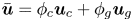 $\bar {\boldsymbol {u}} = \phi _{{c}} \boldsymbol {u}_{{c}} + \phi _{{g}} \boldsymbol {u}_{{g}}$ we can derive the continuity equation of the two-component model, equation (2.13).
The sum of the momentum conservation equations (2.2) and (2.4) is slightly more complex and approximations are required due to nonlinearities. Therefore, we will cover each term individually in the following. The sum of the time derivatives of equations (2.2) and (2.4) can be simplified with the definition of the volume-averaged velocity  $\bar {\boldsymbol {u}}$, the local density
  $\rho = \phi _{{c}} \rho _{{c}} + \phi _{{g}} \rho _{{g}}$ and the relative velocity
  $\boldsymbol {u}_{{r}} = \boldsymbol {u}_{{g}} - \boldsymbol {u}_{{c}}$ to give
 \begin{align} \frac{\partial}{\partial t} (\phi_{{c}} \rho_{{c}} \boldsymbol{u}_{{c}} + \phi_{{g}} \rho_{{g}} \boldsymbol{u}_{{g}} ) &=\frac{\partial}{\partial t} (\phi_{{c}} \rho_{{c}} (\bar{\boldsymbol{u}}-\phi_{{g}}\boldsymbol{u}_{{r}} ) +\phi_{{g}} \rho_{{g}} (\bar{\boldsymbol{u}}+\phi_{{c}} \boldsymbol{u}_{{r}} ) ) \nonumber\\ & =\frac{\partial \rho\bar{\boldsymbol{u}}}{\partial t} + \frac{\partial }{\partial t} (\phi_{{g}} \phi_{{c}} \boldsymbol{u}_{{r}} (\rho_{{g}}-\rho_{{c}} ) ) \approx \frac{\partial \rho\bar{\boldsymbol{u}}}{\partial t}. \end{align}
The second term in (A2) vanishes if the relative velocity is zero or if the phase densities are equal. The two-component model assumes that phase velocities are equal (equation (2.11)) and the second term can be neglected. The error in the momentum conservation is expected to be small in relation to limitations of the incompressible rheology.
The sum of the convective fluxes follows a similar pattern,
 \begin{align}
&\boldsymbol{\nabla}\boldsymbol{\cdot} (\phi_{{c}}
\rho_{{c}}
\boldsymbol{u}_{{c}}\otimes\boldsymbol{u}_{{c}}+\phi_{{g}}
\rho_{{g}} \boldsymbol{u}_{{g}}\otimes\boldsymbol{u}_{{g}}
) \nonumber\\ &\quad= \boldsymbol{\nabla}\boldsymbol{\cdot}
(\phi_{{c}} \rho_{{c}} (\bar{\boldsymbol{u}}-\phi_{{g}}
\boldsymbol{u}_{{r}} )\otimes
(\bar{\boldsymbol{u}}-\phi_{{g}} \boldsymbol{u}_{{r}}
)+\phi_{{g}} \rho_{{g}} (\bar{\boldsymbol{u}}+\phi_{{c}}
\boldsymbol{u}_{{r}} )\otimes
(\bar{\boldsymbol{u}}+\phi_{{c}} \boldsymbol{u}_{{r}} ) )
\nonumber\\ &\quad=\boldsymbol{\nabla}\boldsymbol{\cdot}
(\rho\bar{\boldsymbol{u}}\otimes\bar{\boldsymbol{u}} ) +
\boldsymbol{\nabla} \boldsymbol{\cdot} (\phi_c \phi_g (\bar{\boldsymbol{u}} \otimes \boldsymbol{u}_r + \boldsymbol{u}_r \otimes \bar{\boldsymbol{u}} ) (\rho_g - \rho_c) )\nonumber\\
&\qquad+ \boldsymbol{\nabla}\boldsymbol{\cdot} (\phi_{{c}}
\phi_{{g}} \boldsymbol{u}_{{r}}\otimes\boldsymbol{u}_{{r}}
(\phi_{{g}} \rho_{{c}}+\phi_{{c}} \rho_{{g}} ) )
\nonumber\\ &\quad\approx
\boldsymbol{\nabla}\boldsymbol{\cdot}
(\rho\bar{\boldsymbol{u}}\otimes\bar{\boldsymbol{u}} ).
\end{align}
\begin{align}
&\boldsymbol{\nabla}\boldsymbol{\cdot} (\phi_{{c}}
\rho_{{c}}
\boldsymbol{u}_{{c}}\otimes\boldsymbol{u}_{{c}}+\phi_{{g}}
\rho_{{g}} \boldsymbol{u}_{{g}}\otimes\boldsymbol{u}_{{g}}
) \nonumber\\ &\quad= \boldsymbol{\nabla}\boldsymbol{\cdot}
(\phi_{{c}} \rho_{{c}} (\bar{\boldsymbol{u}}-\phi_{{g}}
\boldsymbol{u}_{{r}} )\otimes
(\bar{\boldsymbol{u}}-\phi_{{g}} \boldsymbol{u}_{{r}}
)+\phi_{{g}} \rho_{{g}} (\bar{\boldsymbol{u}}+\phi_{{c}}
\boldsymbol{u}_{{r}} )\otimes
(\bar{\boldsymbol{u}}+\phi_{{c}} \boldsymbol{u}_{{r}} ) )
\nonumber\\ &\quad=\boldsymbol{\nabla}\boldsymbol{\cdot}
(\rho\bar{\boldsymbol{u}}\otimes\bar{\boldsymbol{u}} ) +
\boldsymbol{\nabla} \boldsymbol{\cdot} (\phi_c \phi_g (\bar{\boldsymbol{u}} \otimes \boldsymbol{u}_r + \boldsymbol{u}_r \otimes \bar{\boldsymbol{u}} ) (\rho_g - \rho_c) )\nonumber\\
&\qquad+ \boldsymbol{\nabla}\boldsymbol{\cdot} (\phi_{{c}}
\phi_{{g}} \boldsymbol{u}_{{r}}\otimes\boldsymbol{u}_{{r}}
(\phi_{{g}} \rho_{{c}}+\phi_{{c}} \rho_{{g}} ) )
\nonumber\\ &\quad\approx
\boldsymbol{\nabla}\boldsymbol{\cdot}
(\rho\bar{\boldsymbol{u}}\otimes\bar{\boldsymbol{u}} ).
\end{align}
The second and third terms vanish if the relative velocity is zero. Notably, only the second term vanishes if the phase densities are equal due to the nonlinearity in the convection term. For the approximation of the two-component model, it is sufficient to recover the first term, as the relative velocity is neglected.
The terms on the right-hand sides of equations (2.2) and (2.4) can be summed up without further assumptions,
 \begin{gather} \boldsymbol{\nabla}\boldsymbol{\cdot} (\phi_{{c}} {\boldsymbol{\mathsf{T}}}_{{c}} + \phi_{{g}} {\boldsymbol{\mathsf{T}}}_{{g}} ) = \boldsymbol{\nabla}\boldsymbol{\cdot}{\boldsymbol{\mathsf{T}}}, \end{gather}
 \begin{gather}\phi_{{c}} \boldsymbol{\nabla} p+\phi_{{g}} \boldsymbol{\nabla} p + \boldsymbol{\nabla}\,p_{{s}} = \boldsymbol{\nabla} p_{{tot}}, \end{gather}
 \begin{gather}\phi_{{c}} \rho_{{c}} \boldsymbol{g}+\phi_{{g}} \rho_{{g}} \boldsymbol{g} = \rho \boldsymbol{g}, \end{gather}
 \begin{gather}k_{{gc}} (\boldsymbol{u}_{{g}}-\boldsymbol{u}_{{c}} ) + k_{{gc}} (\boldsymbol{u}_{{c}}-\boldsymbol{u}_{{g}} ) = 0, \end{gather}
and the momentum conservation equation of the two-component model, equation (2.12), can be assembled.
Appendix B. Sensitivity study
The numerical models require a wide range of parameters. Most parameters are physical and can be derived from experiments and the literature. However, some parameters are purely numerical and their values cannot be derived from experiments. The following parameter study was used to derive numerical parameters that have been applied in the simulations. The most influential numerical parameters are the grid size  ${\rm \Delta} x$, the Courant number
  ${CFL}^{{diff}}$, related to the time step
  ${\rm \Delta} t$, and the maximum viscosity
  $\nu _{max}$. Furthermore, the effect of dynamic friction, i.e. the difference between a constant friction coefficient
  $\mu$ and the
  $\mu (I)$ or
  $\mu (J)$-rheology, is investigated. The applied model and the flow regime (subaerial or subaquatic, dense or loose) are given in the captions for each of the following figures.
B.1. Influence of the maximum viscosity
The maximum viscosity is one of the most influential numerical parameters in the applied model. It should be reasonably high to mimic solid behaviour, but as small as possible to improve numerical stability and to keep computational expense low. A reasonable limit can be found by investigating the dimensionless governing equations, in which the respective scales are isolated. The momentum conservation of the Navier–Stokes equations can be written as
 \begin{equation} \frac{\partial \boldsymbol{u}}{\partial t} + \boldsymbol{\nabla}\boldsymbol{\cdot}(\boldsymbol{u}\otimes\boldsymbol{u}) ={-}\frac{1}{\rho} \boldsymbol{\nabla}\,p + \frac{1}{2} \nu \boldsymbol{\nabla}^2 \boldsymbol{u} + \boldsymbol{g}\end{equation}
for a single incompressible Newtonian fluid with density  $\rho$ and constant viscosity
  $\nu$. By scaling space with the height of the slide
  $H$, the velocity with the respective free-fall velocity
  $\sqrt {|\boldsymbol {g}| H}$, the time with the free-fall time
  $\sqrt {H/|\boldsymbol {g}|}$, and the pressure with the respective hydrostatic pressure
  $\rho |\boldsymbol {g}| H$, the dimensionless variables (marked with a hat) can be established as
 \begin{gather} \boldsymbol{x} = H \hat{\boldsymbol{x}}, \end{gather}
 \begin{gather}\boldsymbol{\nabla} = \frac{1}{H} \hat{\boldsymbol{\nabla}} = \frac{1}{H} \left(\frac{\partial}{\partial\hat{\boldsymbol{x}}}, \frac{\partial}{\partial\hat{\boldsymbol{y}}}, \frac{\partial}{\partial\hat{\boldsymbol{z}}}\right)^\textrm{T}, \end{gather}
 \begin{gather}\boldsymbol{u} = \sqrt{|\boldsymbol{g}| H}\,\hat{\boldsymbol{u}}, \end{gather}
 \begin{gather}t = \sqrt{\frac{H}{|\boldsymbol{g}|}}\,\hat{t}, \end{gather}
 \begin{gather}p = \rho |\boldsymbol{g}| H \hat{p}. \end{gather}
Introducing the dimensionless variables into the momentum conservation equation and dividing by  $|\boldsymbol {g}|$ yields
 \begin{equation} \frac{\partial \hat{\boldsymbol{u}}}{\partial \hat{t}} + \hat{\boldsymbol{\nabla}}\boldsymbol{\cdot}(\hat{\boldsymbol{u}}\otimes\hat{\boldsymbol{u}}) ={-}\hat{\boldsymbol{\nabla}} \hat{p} + \sqrt{\frac{1}{|\boldsymbol{g}| H^3}}\,\nu \hat{\boldsymbol{\nabla}}^2 \hat{\boldsymbol{u}} + \frac{\boldsymbol{g}}{|\boldsymbol{g}|}. \end{equation}
In the case of a solid-like behaviour, the viscous term should dominate over all other terms. All terms, except for the viscous term, are of order one and we can deduce that the inequality
 \begin{equation} \sqrt{\frac{1}{|\boldsymbol{g}| H^3}}\,\nu_{{max}} > \frac{1}{\varepsilon} \end{equation}
should be fulfilled to simulate the behaviour of a solid. In the above,  $\varepsilon$ is a small dimensionless number, indicating the magnitude of viscous stresses over other terms. The viscosity that is required for a solid-like behaviour can be calculated as
 \begin{equation} \nu_{{max}} > \frac{1}{\varepsilon} \sqrt{|\boldsymbol{g}| H^3}, \end{equation}
as a function of the respective scales by choosing the magnitude of viscous stresses over other terms,  $\varepsilon$. The required magnitude for
  $\varepsilon$ can be estimated by conducting a numerical sensitivity analysis.
Variations of  $\nu _{{max}}$ (and thus
  $\varepsilon$) are presented in figure 16 for the subaerial case at
  $t=0.8\ \textrm {s}$, using the two-component model. The value of
  $\nu _{{max}} = 1\ \textrm {m}^{2}\ \textrm {s}^{-1}$ is adequate for this example and the left side of the pile stays nearly static as is the case in the experiment. The respective value for the dimensionless scaling factor
  $\varepsilon$ follows as
  $0.1$ (
 $H = 0.1\ \textrm {m}$,
  $|\boldsymbol {g}|\approx 10\ \textrm {m}\ \textrm {s}^{2}$), indicating that viscous forces have to be approximately
  $10$ times higher than all other contributions to the momentum conservation equation. For lower viscosities, the pile is notably deformed and shows no stable regions and no granular characteristics. Rather, the pile shows the characteristics of a viscoplastic fluid (see rheology comparisons by Lagrée et al. (Reference Lagrée, Staron and Popinet2011)), which indicates that the viscosity threshold was dominating the simulation. Notably, cases with high maximum viscosity are stable after
  $t=0.4\ \textrm {s}$ while cases with low maximum viscosity keep flowing beyond
  $t=0.8\ \textrm {s}$. For an application of granular rheologies in OpenFOAM, we suggest a maximum viscosity following (2.28) with
  $\varepsilon = 1/10$.

Figure 16. Pile shape at  $t=0.8\ \textrm {s}$ of the subaerial granular collapse with various values for
  $\nu _{{max}}$ using the two-component model. The high influence of this numerical parameter and the unphysical effect of low values is clearly visible. The dashed black line shows the final pile shape of the experiment for comparison. The two-phase model behaves similarly.
B.2. Grid sensitivity
The grid sensitivity is an important issue for complex flow models, and we provide a full grid sensitivity analysis for the multicomponent and the multiphase models. The grid sensitivity study for the multicomponent model is solely conducted for the subaerial case because the mechanics of this model is similar in all cases. The final pile shape of the investigated case is shown in figure 17 for various grid resolutions. This model reacts very robustly to coarse grids, and 30 cells along the pile height are sufficient to get accurate results for the final pile shape.

Figure 17. Grid sensitivity of the two-component model for the subaerial case. The model behaves similarly in the subaquatic cases. The black dashed line shows the experimental final pile shape for reference.
The two-phase model is more complex in terms of grid sensitivity. Three different failure mechanisms of the granular column can be observed in the simulations with the two-phase model. The three mechanisms react differently to a variation of the grid resolution. In some cases, the model reacts very sensitively to coarse grids and a grid refinement study should always be performed when applying this model. Figure 18 shows the grid convergence analysis for the subaerial, the subaquatic dense and subaquatic loose cases. The two-phase model is slightly more sensitive to coarse grids than the two-component model in the subaerial case; see figure 18(a). The problematic area is the thin flow front and the issue is probably related to the mixed role of the phase-fraction field.

Figure 18. Grid sensitivity of the two-phase model for the subaerial case (a), the dense subaquatic case (b) and the subaquatic loose case (c). The black dashed lines show the experimental final pile shapes for reference.
The two-phase model is very sensitive to coarse grids in the subaquatic dense case; see figure 18(b). Breaching of a thin layer of grains on the unsupported side of the column leads to a reduced phase fraction in cells that contain the slide surface. This reduces the effective pressure in all of those cells and further the shear strength, accelerating the collapse. The result is a mesh dependence of the final pile shape and the collapse velocity. The mesh had to be refined down to a cell size of  $0.0005\ \textrm {m}$ to achieve accurate results. Notably, the difference between the smallest two cell sizes is still remarkable at the front of the collapse. An additional refinement step would be desirable, but this would have exhausted the available computational resources.
The loose subaquatic case can be simulated with good accuracy on a relatively coarse mesh as shown in figure 18(c). This is not surprising, as the failure mechanism and flow pattern are much simpler. In particular, the effective pressure discontinuity at the free surface is weaker than in the dense case and thus requires a smaller grid resolution.
B.3. Time-step duration sensitivity
The time-step duration is investigated similarly as the grid resolution. The time-step duration is not fixed but is adapted to velocity ( ${CFL}^{\textrm {conv}}$) and viscosity (
 ${CFL}^{{diff}}$), relative to the grid size. The viscous contribution to the CFL number is always much bigger in the investigated cases and the time-step sensitivity study was conducted based on this value. Notably, stability can be guaranteed only for
  ${CFL}^{{diff}} <1$. However,
  ${CFL}^{{diff}}$ allows only an estimation of the stability and in some cases larger time steps are possible.
The two-component solver can operate in two modes, using a full momentum predictor step or a reduced momentum predictor step. The full momentum predictor step solves the full linearized system of the discretized momentum conservation equation. The reduced momentum predictor step calculates an explicit prediction of the velocity field based on the velocity field of the last time step. This has a substantial influence on the stability when viscous stresses are dominant.
Figure 19(a) shows the final pile shape for various time-step durations and the full momentum predictor step in the two-component model. Notably, oscillations in pressure can already be seen at  ${CFL}^{{diff}} = 2$ (not shown) and they grow substantially for higher
  ${CFL}^{{diff}}$. The pressure oscillations start to influence the pile shape at
  ${CFL}^{{diff}} = 10$ and the pile is completely distorted for
  ${CFL}^{{diff}} = 100$.

Figure 19. Sensitivity of the two-component subaerial model on the time-step duration, expressed by the viscous CFL number. The solver was operated with the full momentum predictor (a) and the reduced momentum predictor (b).
The two-component model is more robust to larger time steps when operating with the reduced momentum predictor step; see figure 19(b). Pressure oscillations start approximately at  ${CFL}^{{diff}} = 100$ and the first influence on the slide geometry can be observed at
  ${CFL}^{{diff}} = 1000$. Anyway, it is recommended to run the two-component model with small enough time steps to prevent pressure oscillations, ideally at
  ${CFL}^{{diff}} = 1$, as done in this work.
The two-phase model reacts less sensitively to large time-step durations. In fact, simulations were stable up to  ${CFL}^{{diff}} = 1000$. No pressure oscillations could be observed and the final pile shape is nearly unaffected for all cases; see figure 20. However, the accuracy became worse for large time-step durations and we observed a slower initial acceleration for
  ${CFL}^{{diff}} = 1000$. No subaquatic simulations with the two-phase model and
  ${CFL}^{{diff}} = 1$ have been conducted, as this would have exhausted the computational resources.

Figure 20. Sensitivity of the two-phase model on the time-step duration, expressed by the viscous CFL number in the subaerial case (a), the subaquatic dense case (b) and the subaquatic loose case (c).
B.4. Influence of dynamic friction and wall friction
The effect of the dynamic increase of friction following the  $\mu (I)$-rheology and the effect of the reduced wall friction were investigated with both models. Results are shown in figure 21(a) for the two-component model and in figure 21(b) for the two-phase model. The models do not react sensitively to the variation of the friction model and the basal friction coefficient. The runout is slightly underestimated in simulations with the
  $\mu (I)$-rheology on a rough surface. However, the introduction of the smooth surface elongates the runout and the simulations fit the experiment well. Simulations with a constant friction coefficient on a rough surface also fit the experiment well; simulations with constant friction coefficient on a smooth surface overestimate the runout.

Figure 21. Influence of dynamic friction, dynamic effective pressure and wall friction on the final pile shape in the two-component model (a) and the two-phase model (b).
The dynamic contribution to the effective pressure and friction is imperative for simulations at low Stokes numbers. Figure 22 shows the dense and loose subaquatic two-phase simulations with critical state theory and  $\mu (J)$,
  $\phi (J)$-theory. The outrun cannot be controlled without the dynamic contributions of the
  $\mu (J)$,
  $\phi (J)$-theory and exceeds the final runout very quickly.

Figure 22. The dense granular collapse at  $t=6.0\ \textrm {s}$ (a) and the loose granular collapse at
  $t=0.65\ \textrm {s}$ (b), simulated with critical state theory and
  $\mu (J)$,
  $\phi (J)$-rheology. The dashed black line shows the final experimental pile shape. The simulations with critical state theory clearly exceed the experiment early in the simulation.
B.5. Influence of the creep shear rate
The influence of the creep shear rate  $S_0$ is shown in figure 23 for the subaquatic dense case. Figure 23 shows an early time step at
  $t=1.0\ \textrm {s}$ and the final pile shape at
  $t=10\ \textrm {s}$. A reduction of the creeping shear rate from
  $5\ \textrm {s}^{-1}$ to
  $1\ \textrm {s}^{-1}$ leads to a slower initial collapse of the column. The delayed collapse is desirable and brings the simulation closer to the experiment. However, the low value for
  $S_0$ leads to oscillations in the particle pressure because the simulation accelerates and reaches shear rates beyond
  $S_0$ too quickly. The simulation with
  $S_0 = 5\ \textrm {s}^{-1}$ shows no oscillations and has thus been utilized in the main part of this work. Notably, a smaller time-step duration will allow smaller values for
  $S_0$, but for an increased computational cost. The final pile shape is barely affected by the change in
  $S_0$.

Figure 23. Influence of the creep shear rate  $S_0$ on the pile shape. Two time steps are shown,
  $t=1\ \textrm {s}$ (continuous) and
  $t=10\ \textrm {s}$ (dashed). The black dashed line shows the final experimental pile shape.


 Open access