


INTRODUCTION
Conversion of natural habitats is one of the biggest threats to global biodiversity (Pereira et al. Reference Pereira, Leadley, Proenca, Alkemade, Scharlemann, Fernandez-Manjarres, Araujo, Balvanera, Biggs, Cheung, Chini, Cooper, Gilman, Guenette, Hurtt, Huntington, Mace, Oberdorff, Revenga, Rodrigues, Scholes, Sumaila and Walpole2010), and designation of protected areas (PAs) is one of the most widespread approaches to mitigating this threat. It is now well established that PAs can be effective at reducing rates of loss of natural land cover (e.g. Andam et al. Reference Andam, Ferraro, Pfaff, Sanchez-Azofeifa and Robalino2008; Gaveau et al. Reference Gaveau, Epting, Lyne, Linkie, Kumara, Kanninen and Leader-Williams2009; Selig & Bruno Reference Selig and Bruno2010; Beresford et al. Reference Beresford, Eshiamwata, Donald, Balmford, Bertzky, Brink, Fishpool, Mayaux, Phalan, Simonetti and Buchanan2013; Geldmann et al. Reference Geldmann, Barnes, Coad, Craigie, Hockings and Burgess2013; Butsic et al. Reference Butsic, Baumann, Shortland, Walker and Kuemmerle2015), but that they vary greatly in the extent to which they achieve this (Andam et al. Reference Andam, Ferraro, Pfaff, Sanchez-Azofeifa and Robalino2008; Joppa & Pfaff Reference Joppa and Pfaff2011; Francoso et al. Reference Francoso, Brandao, Nogueira, Salmona, Machado and Colli2015; Paiva et al. Reference Paiva, Brites and Machado2015). Targets for expanding PA networks are often based largely or solely on the area covered. Aichi Target 11 of the Convention on Biological Diversity (CBD) sets targets for the coverage of land and sea by PAs, but then simply states that these need to be effectively managed. It does not set a target against which this effectiveness can be assessed. Thus, designation alone is an insufficient measure of the effectiveness of a PA network. Conservation also requires an understanding of the effectiveness of protection and how this varies between locations. Estimates of both extent and effectiveness are needed in order to develop effective networks of PAs capable of meeting conservation targets at local to global scales.
As there have been inconsistencies in the way that terms such as ‘impact’ and ‘effectiveness’ of PAs have been applied and interpreted across different studies, we identify three key elements determining the overall impact of a PA: (i) the conservation value of the site, which is a function of the biota it holds and its area; (ii) the degree of threat to the site; and (iii) the degree to which that threat is reduced by designation (i.e. the effectiveness of protection).
Analysis of the effectiveness of PAs is not as simple as comparing rates of change with surrounding areas or randomly chosen points due to the non-random distribution of PAs within the landscape (Joppa & Pfaff Reference Joppa and Pfaff2009; Nelson & Chomitz Reference Nelson and Chomitz2011; Joppa & Pfaff Reference Joppa and Pfaff2011; Beresford et al. Reference Beresford, Eshiamwata, Donald, Balmford, Bertzky, Brink, Fishpool, Mayaux, Phalan, Simonetti and Buchanan2013; Pfaff et al. Reference Pfaff, Robalino, Sandoval and Herrera2015a) and to other effects, such as the potential ‘leakage’ of conversion from within to outside the PA boundary (Ewers & Rodrigues Reference Ewers and Rodrigues2008; Robalino et al. Reference Robalino, Pfaff and Villalobos2015). Consequently, it is necessary to match protected (treatment) and unprotected (control) sites in order to control for confounding effects that might drive the likelihood of both designation and conversion. Matching by appropriate characteristics that may influence these rates can effectively control for locational bias in the siting of PAs (Joppa & Pfaff Reference Joppa and Pfaff2011; Nelson & Chomitz Reference Nelson and Chomitz2011; Beresford et al. Reference Beresford, Eshiamwata, Donald, Balmford, Bertzky, Brink, Fishpool, Mayaux, Phalan, Simonetti and Buchanan2013).
A number of studies have been undertaken on regional to global scales in which sites have been matched by variables such as ecoregion, rainfall, agricultural suitability, elevation, slope and distance from roads and urban areas, with an consensus emerging that impacts in terms of avoided conversion are greatest on flatter land and at sites near to roads and cities (Joppa & Pfaff Reference Joppa and Pfaff2011; Pfaff et al. Reference Pfaff, Robalino, Sandoval and Herrera2015a). The effectiveness of PAs in meeting their potential can be influenced by a range of factors, such the type of designation and the level and effectiveness of enforcement, as well as the siting and accessibility of the PA (Nelson & Chomitz Reference Nelson and Chomitz2011; Pfaff et al. Reference Pfaff, Robalino, Lima, Sandoval and Herrera2014; Pfaff et al. Reference Pfaff, Robalino, Herrera and Sandoval2015b).
Even in studies in which matching is used to assess more accurately PA impacts, it can still be difficult to disentangle the relative effects of different elements of impact, as there are often complex interactions between them (Geldmann et al. Reference Geldmann, Barnes, Coad, Craigie, Hockings and Burgess2013). In particular, there are often negative correlations between threat and effectiveness, with protection being more effective on sites with lower impact in terms of avoided conversion (e.g. Ahrends et al. Reference Ahrends, Burgess, Milledge, Bulling, Fisher, Smart, Clarke, Mhoro and Lewis2010; Boakes et al. Reference Boakes, Mace, McGowan and Fuller2010; Brun et al. Reference Brun, Cook, Lee, Wich, Koh and Carrasco2015). On the other hand, threat and conservation value are often positively correlated, with sites containing the most threatened habitats being considered to be those of highest conservation value.
These relationships are further complicated by the fact that a single variable such as slope, elevation or accessibility can often influence – or correlate with – more than one element of impact. For example, protected sites on steeper slopes may be more effective than those on flatter ground, but may have a lower impact in terms of avoided conversion if rates of conversion are already low because of the steeper ground (Joppa & Pfaff Reference Joppa and Pfaff2011). Depending on how conservation value is measured, the tendency for low rates of conversion may mean that the site is considered of high conservation value (i.e. pristine condition) or of relatively low value (if low conversion rates result in it being relatively abundant in the landscape).
Much conservation effort is focused on the designation and management of PAs across the globe, so a better understanding of the factors influencing their effectiveness in reducing the conversion of natural land cover is needed in order to assess the relative benefits of existing PAs and to identify sites whose future protection would bring the greatest benefits. This is especially true given that they represent the mechanism through which so many conservation issues are tackled. Of the 20 Aichi Biodiversity Targets set under the CBD, Target 11 relates directly to the designation of PAs. PA networks can also make a major contribution to other targets (e.g. Target 1, relating to the awareness of people of the values of biodiversity; Target 5, relating to loss of natural habitats; Target 12, on preventing the extinction of known threatened species; Target 14, on the preservation of ecosystem services; and Target 15, on carbon storage; Scharlemann et al. Reference Scharlemann, Kapos, Campbell, Lysenko, Burgess, Hansen, Gibbs, Dickson and Miles2010; Beresford et al. Reference Beresford, Buchanan, Sanderson, Jefferson and Donald2016). They also have a recognized role to play in mitigating the impacts of climate change on people and biodiversity (Loarie et al. Reference Loarie, Duffy, Hamilton, Asner, Field and Ackerly2009; Thomas & Gillingham Reference Thomas and Gillingham2015).
In a previous study (Beresford et al. Reference Beresford, Eshiamwata, Donald, Balmford, Bertzky, Brink, Fishpool, Mayaux, Phalan, Simonetti and Buchanan2013), we focused on measuring the impact of protection in terms of avoided conversion by comparing rates of loss of natural land cover between protected and unprotected sites of recognized conservation value (Important Bird and Biodiversity Areas (IBAs)) in Africa. IBAs are sites of global significance for the conservation of the world's birds, identified using semi-quantitative criteria (Fishpool & Evans Reference Fishpool and Evans2001), and are Key Biodiversity Areas (IUCN 2016). The most prevalent threats to African IBAs are associated with land-cover change (Buchanan et al. Reference Buchanan, Donald, Fishpool, Arinaitwe, Balman and Mayaux2009). Use of this set of sites eliminates from our study the influence of PAs of relatively low conservation value that were designated primarily because of their low opportunity cost and low likelihood of conversion.
We previously established that protection is effective at reducing – but not halting – land-cover change on protected IBAs compared to unprotected IBAs (Beresford et al. Reference Beresford, Eshiamwata, Donald, Balmford, Bertzky, Brink, Fishpool, Mayaux, Phalan, Simonetti and Buchanan2013). Here, we develop this work by using the same database of spatially explicit information on land-cover change in and around African IBAs in order to identify the characteristics of points that were (and were not) converted during the study. In doing so, we hope to identify potential drivers of conversion and enable proactive conservation. This information could be used to better target monitoring of sites. Additionally, and perhaps more importantly, we could identify areas most at risk from habitat loss and potentially increase the rapidity with which threats are tackled on the ground in these places. We produce statistical models of relationships (generalized linear mixed models (GLMMs)) and consider the interaction between correlate variables and whether or not the point is protected. By examining output-fitted relationships, we can determine whether the form of the relationship varies within and outside PAs. This allows differing conservation strategies to be developed within and outside PAs, if appropriate. By investigating changes on sites of objectively defined high conservation importance (IBAs), this is the first study to control for variation in potential impact in terms of conservation value, as well as avoided conversion, which we account for using site-level matching.
METHODS
Site selection
Protected and unprotected IBAs were matched at the site level to reduce the known problem of the non-random distributions of PAs, which are often designated in remote and inaccessible areas where the risk of damage is inherently lower than in more accessible areas (Joppa & Pfaff Reference Joppa and Pfaff2009). Matching ensures that protected sites are compared with unprotected sites with a comparable risk of sustaining damage by controlling for some of the most likely correlates of environmental risk. Full details of the selection process are given in Beresford et al. (Reference Beresford, Eshiamwata, Donald, Balmford, Bertzky, Brink, Fishpool, Mayaux, Phalan, Simonetti and Buchanan2013). This selection process resulted in a set of 54 protected and 49 unprotected IBAs from the 793 IBAs in continental sub-Saharan Africa and Madagascar for which digital boundaries were available. Our sample of 103 sites differs slightly from Beresford et al. (Reference Beresford, Eshiamwata, Donald, Balmford, Bertzky, Brink, Fishpool, Mayaux, Phalan, Simonetti and Buchanan2013) because we include IBAs from countries for which only a single site was selected by the matching process. We obtained site protection status by intersecting the boundaries of all IBAs with the boundaries of all 1580 nationally designated PAs in Africa from the World Database on Protected Areas (International Union for Conservation of Nature (IUCN) categories I to VI) that had digitized boundaries (IUCN & UNEP-WCMC 2010). We defined protected IBAs as those that fell wholly or mostly (>90%) within the boundaries of PAs that had been designated before 1985. Partially (<90%) protected sites and those whose protection status changed immediately before or during the assessment period were excluded from the selection process. We defined unprotected IBAs as those that did not overlap any PAs, irrespective of PA designation date. We excluded from our analysis all IBAs smaller than 10 km2, because the number of points at which we could have assessed land cover would have been small. We matched protected and unprotected IBAs using the command ‘subclass’ in the MatchIt package (Ho et al. Reference Ho, Imai, King and Ferrer2011) in R (R Development Core Team 2010). We matched sites on the basis of area, mean altitude (both from BirdLife International (2011)), mean distance from roads (National Imagery and Mapping Agency 2000), mean human population density (CIESIN & CIAT 2005) and the most extensive GLC2000 land-cover class in the IBA (Mayaux et al. Reference Mayaux, Bartholomé, Fritz and Belward2004). Site-level matching ensured that protected and unprotected IBAs were similar at the landscape level.
Assessment of land-cover change
We used visual interpretation of satellite imagery to assess dominant land cover within 300 × 300-m sample boxes (‘points’) in each IBA and in a surrounding 20-km buffer using a dedicated graphical user interface (Bastin et al. Reference Bastin, Buchanan, Beresford, Pekel and Dubois2013). Points were distributed on a regular grid and spaced 0.5 km apart in IBAs of <50 km2, 1.5 km apart in IBAs of >50 km2 and 3 km apart in the 20-km buffers. Excluding points where cloud-free images were unavailable for any one time period, this gave a total of 20,481 points assessed within IBAs and 17,870 points in their buffers. We recorded land cover at each point once in each of three time periods: 1981–1994, 1995–2004 and 2005–2009. The years of sampling varied according to the availability of high-quality, cloud-free images. Variation between sites in years of sampling was controlled in the analyses by modelling survival of natural land cover as a point-specific exposure period (see below).
For the years from 1981 to 2002, we used freely available imagery from Landsat (http://www.landcover.org; Tucker et al. Reference Tucker, Grant and Dykstra2004). For the years 2003–2009, we used a combination of Landsat imagery (http://glovis.usgs.gov) and purchased Aster images. All images had a spatial resolution of 30 m. We excluded points for which no data were available (because of cloud, poor image quality or the failure of Landsat 7’s scan line corrector after 2003) in one or more of the sampling periods. We also excluded the small number of points in some IBA buffers that overlapped other PAs or IBAs.
The dominant land cover at each point in each time period was allocated to one of 11 broad categories: closed tree cover; open tree cover; mosaic of natural and agricultural vegetation; shrub; herbaceous; tree and shrub crops; arable crops; open water; flooded shrub and herbaceous; urban; and bare (classification based on Di Gregorio & Jansen (Reference Di Gregorio and Jansen2000)). Of these categories, we considered four as ‘non-natural’ land covers: mosaic of natural and agricultural vegetation; tree and shrub crops; arable crops; and urban. The others were considered ‘natural’ land covers. For points at which the initial land cover was closed or open tree cover (forests), subsequent change to any other land cover was counted as conversion. For other natural land covers, only conversion to non-natural land covers was counted as conversion. Across all land-cover types, natural and non-natural land covers could be separated with an estimated accuracy of c. 94%; further details on interpretation and validation are given in Beresford et al. (Reference Beresford, Eshiamwata, Donald, Balmford, Bertzky, Brink, Fishpool, Mayaux, Phalan, Simonetti and Buchanan2013).
Correlates of land-cover change
In addition to the potential correlates of land-cover change used in the initial site matching (area, altitude, distance to roads, human population density and most extensive land cover), we obtained maps of market accessibility (Nelson Reference Nelson2008), elevation (Jenness et al. Reference Jenness, Dooley, Aguilar-Manjarrez and Riva2007), slope (USGS 2006), agricultural suitability (Fischer et al. Reference Fischer, van Velthuizen, Shah and Nachtergaele2002), cropland cover in 1990 (Ramankutty et al. Reference Ramankutty, Evan, Monfreda and Foley2008) and biome (Olson et al. Reference Olson, Dinerstein, Wikramanayake, Burgess, Powell, Underwood, D'amico, Itoua, Strand, Morrison, Colby, Allnutt, Ricketts, Kura, Lamoreux, Wettengel, Hedao and Kassem2001). We included a four-level ‘class’ factor denoting whether a point fell within a protected IBA or its buffer or an unprotected IBA or its buffer, and a covariate indicating the distance of each point from the edge of the IBA, with negative values indicating points within the IBA and positive values indicating points outside the IBA (Beresford et al. Reference Beresford, Eshiamwata, Donald, Balmford, Bertzky, Brink, Fishpool, Mayaux, Phalan, Simonetti and Buchanan2013). A summary of the explanatory variables and their sources is given in Table 1. We included the initial land-cover category at each point as a categorical variable and calculated the proportions of other points within 5 km of each point that were already dominated by non-natural land cover in the initial time period (1981–1994). Spatial data manipulation and processing were undertaken in ArcGIS 10.1. Human population density, slope and altitude were log-transformed prior to analysis.
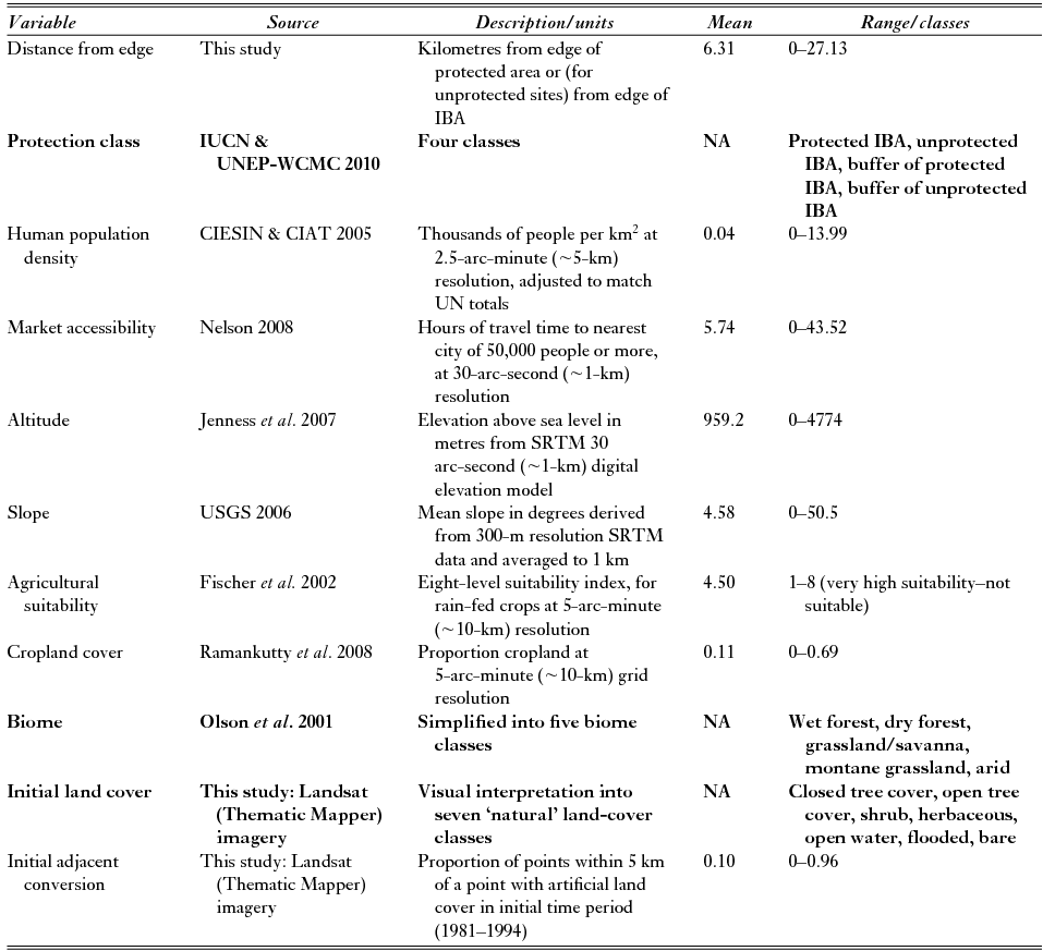
Table 1 Variables used to model land-cover change in and around 103 Important Bird and Biodiversity Areas (IBAs) in Africa. Categorical variables are shown in bold. SRTM = Shuttle Radar Topography Mission.
Data analysis
Land-cover conversion was modelled as a Bernoulli process in a generalized linear mixed model framework using the ‘glmer’ package in R (R Development Core Team 2010). The natural land cover at each point was considered to have survived (if it remained as natural land cover) or not (if it was converted to a non-natural land cover) during a point-specific exposure period, thus controlling for different periods of observation across points. Exposure in the case of points at which natural land cover was not converted was the number of years over which each point was observed (the period between the earliest and latest years of satellite imagery used for each point). For points at which land cover was converted between the first and second or between the second and third assessments, we assumed that loss occurred halfway between the first assessment at which conversion was first recorded and the previous assessment, and calculated the exposure period accordingly.
A binary survival/conversion variable was fitted as the dependent variable and the point-specific exposure period (in years) was fitted as a binomial denominator, allowing us to derive annual survival probabilities that were comparable across all points. Country and site (IBA code) were included in initial models as random effects, either in separate models or as a nested random effect in the same model. Once the best-supported set of random effects had been decided using the ‘anova’ command in ‘glmer’, the best combination of fixed effects was assessed.
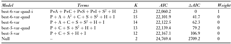
Given the large number of explanatory variables and the many plausible interactions between them, we adopted a pragmatic approach to model selection. First, we fitted all possible combinations of up to a maximum of five explanatory variables (excluding the selected random effects, which remained in all models, and without interactions) using the ‘dredge’ function of the R package ‘MuMIn’ (Bartoń Reference Bartoń2012). These models were ranked by the Akaike information criterion (AIC) and that with the lowest AIC was used as a base from which to assess support for more heavily parameterized models. To the five-or-fewer-variable model selected, we next added the quadratic terms of any covariates in that model; these were retained if they significantly improved the model (reflected in an AIC of 2 or more units lower than the model without the quadratic term(s)). We then added and removed each remaining explanatory variable in turn to select the best-supported model and compared each of these to the previous model using the AIC and likelihood ratio tests in order to assess whether fitting an extra variable to the previous model improved the fit. The process was repeated until the addition of any further variable could not reduce the AIC by at least 2. We then fitted a number of plausible interactions to the model and compared the resulting candidate models using the AIC and likelihood ratio tests. Finally, we assessed whether any simplification of the final model was justified by comparing the AIC of the final model with the AICs of all subsets of that model that lacked each explanatory variable in turn. The relative importance of each predictor was also assessed from this comparison. Once a final model was adopted, we assessed its goodness of fit using the method of Nakagawa and Schielzeth (Reference Nakagawa and Schielzeth2013) with the ‘r.squaredGLMM’ command in ‘MuMIn’.
RESULTS
When accounting for the random effect of IBA, the overall annual survival rate across all natural habitats was 0.996, equating to an overall survival rate of 88.7% over 30 years. The best-supported model of five or fewer variables contained slope, human population density, the four-level protection class, initial land-cover type and the extent of already converted land within 5 km at the start of the observation period (Table 2). This model carried an AIC weight relative to the other competing models of 1, and all other candidate models of five or fewer variables had ΔAIC >37.5 with respect to this model. Likelihood ratio tests supported simplification of this model by reducing the four-level protection class variable to a binary classification in which unprotected IBAs and the buffers of both protected and unprotected IBAs were all classed as ‘unprotected’, and protected IBAs were classed as ‘protected’. A model in which the quadratic term of slope was fitted received greater support than a model without this term, but the same was not true for the quadratic terms of human population density or the proportion of points within 5 km that had been converted to non-natural habitats by the start of the exposure period (Table 2). The addition of altitude and its quadratic term further improved the model (Table 2). The best-supported model was that which also included interactions between protected status and slope, protected status and altitude, protected status and initial conversion and protected status and initial land-cover type (Table 2). Removal of each variable in turn from this model confirmed that no simpler model received greater support, although a model that lacked the interaction between protected status and altitude was within 2 AIC units. The marginal R 2 of the final model (i.e. the variation explained only by the fixed effects) was 0.265, and the conditional R 2 (fixed + random effects) was 0.382. This model indicated that the survival rate of natural land cover increased with increasing slope and altitude and with decreasing human population density, that it was higher in PAs then in unprotected sites, that it varied between major land-cover classes and that it was lower in already heavily converted areas. The interactions indicated that the effects on survival rates of slope, altitude, initial conversion and land-cover types varied between protected and unprotected areas.
Table 2 Model selection table showing the relative support for the null model (random effects only), the best-supported model of five or fewer variables (‘best-5-var’), the same model with quadratic terms fitted for one or more of the covariates decided using the Akaike information criterion (AIC; ‘best-5-var-quad’), the best-supported model that added an extra variable to the previous model (‘best-6-var’), the same model with quadratic terms fitted for the covariate added in the previous step (‘best-6-var-quad’) and the same model with the best-supported combination of interactions assessed by ΔAIC (‘best-6-var-quad-i’). No model with seven or more variables received as much support from the data as the best-supported six-variable models. Important Bird and Biodiversity Area was fitted as a random effect in all models and is not shown. S = slope; A = altitude; H = human population density; I = initial land-cover type; P = protected area status; C = proportion of surrounding points already converted to non-natural land-cover types by start of exposure period; K = number of parameters estimated. Asterisks indicate interactions between variables whose main effects were also included in the model.
Predicted values were generated for each parameter included in the final model by holding each of the other variables in the model, except the binary variable relating to protected status, at its mean or, in the case of factors, at its reference level. This revealed that PAs had lower rates of loss than unprotected areas, but the interactions in the model indicated that this pattern varied across the range of values of other parameters (Fig. 1). Survival of natural habitats increased with increasing slope and altitude, and at high values of both there was little difference between protected and unprotected areas. Survival declined with increasing human population density and with the amount of adjacent land that had already been converted by the start of the observation period. There was little effect of protected status on subsequent rates of loss of natural land cover where land conversion of nearby cells was already high at the start of the exposure period (Fig. 1). Survival varied by major land-cover type, as did the relative benefits of protected status within land-cover types; closed and open forest suffered the greatest overall rates of loss, but the difference between rates of loss in protected and unprotected IBAs was greater in these habitats than was the case in other habitats, indicating a greater impact of PAs in terms of avoided conversion (Fig. 2).
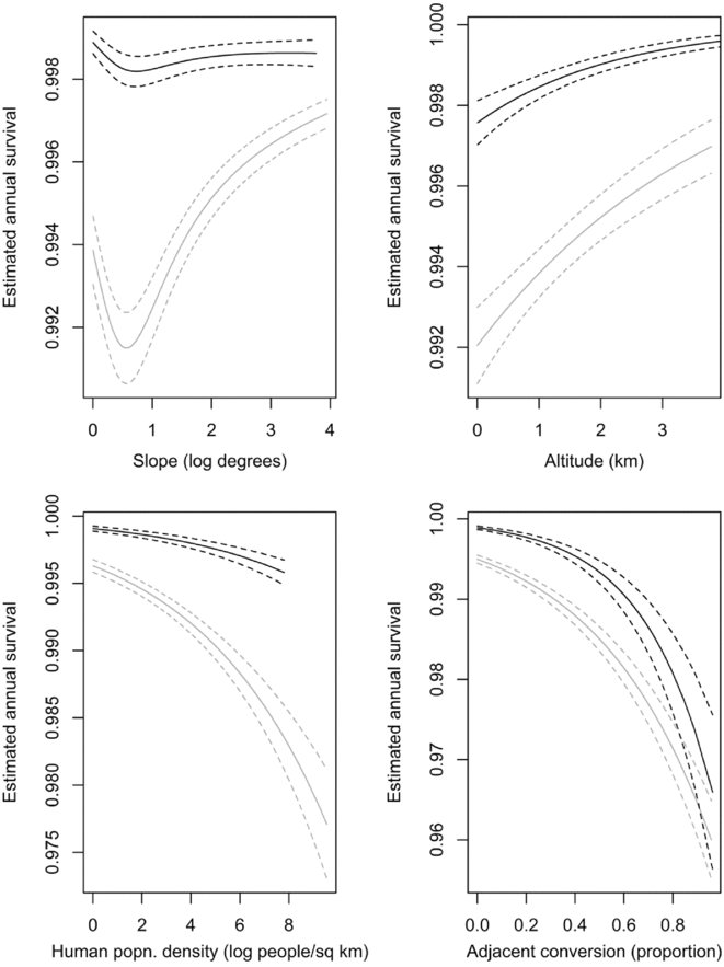
Figure 1 Variation in modelled values (±1 SE) of annual survival rate of natural habitats with slope, altitude, human population density and the amount of conversion that had already taken place by the start of the observation period. Grey = unprotected sites; black = protected areas. Curves were generated using the best-supported model in Table 2 fitted to data in which all variables except the covariate of interest and protected area status were constrained to their mean or reference values.
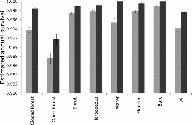
Figure 2 Estimates of annual survival of each of seven broad natural land-cover classes and of all land-cover types combined (±1 SE). Grey = unprotected sites; black = protected sites. Estimates were derived using the best-supported model in Table 2 fitted to data in which all variables except land-cover class and protected area status (or just protected area status in the case of ‘All’) were constrained to their mean or reference values.
DISCUSSION
Our analyses identify a number of environmental and anthropic correlates of natural land-cover conversion, which have additive and sometimes interactive effects. Slope, altitude, human population density and initial adjacent conversion prior to the exposure period were all retained in the final model. In addition, as shown by Beresford et al. (Reference Beresford, Eshiamwata, Donald, Balmford, Bertzky, Brink, Fishpool, Mayaux, Phalan, Simonetti and Buchanan2013), rates of conversion differed significantly between land-cover types.
Our results also confirm many previous assessments (e.g. Andam et al. Reference Andam, Ferraro, Pfaff, Sanchez-Azofeifa and Robalino2008; Gaveau et al. Reference Gaveau, Epting, Lyne, Linkie, Kumara, Kanninen and Leader-Williams2009; Selig & Bruno Reference Selig and Bruno2010; Geldmann et al. Reference Geldmann, Barnes, Coad, Craigie, Hockings and Burgess2013; Butsic et al. Reference Butsic, Baumann, Shortland, Walker and Kuemmerle2015), including our own analysis of these data (Beresford et al. Reference Beresford, Eshiamwata, Donald, Balmford, Bertzky, Brink, Fishpool, Mayaux, Phalan, Simonetti and Buchanan2013), in showing that protection significantly reduces conversion. Rates of conversion in PAs were less than half those in unprotected areas, even when accounting for a range of covariates. However, the beneficial effects of PAs are not universal (e.g. Western et al. Reference Western, Russell and Cuthill2009; Brun et al. Reference Brun, Cook, Lee, Wich, Koh and Carrasco2015; Wendland et al. Reference Wendland, Baumann, Lewis, Sieber and Radeloff2015), and the extent to which protection yields net conservation gains varies greatly, even within relatively small regions (Paiva et al. Reference Paiva, Brites and Machado2015).
We found that the net impact of protection, in terms of the difference in land-cover conversion rates between protected and unprotected areas (i.e. avoided conversion), declined with both slope and altitude (Fig. 1), such that on steeper slopes and at higher altitudes, the annual survival rates of natural land cover in protected and unprotected sites converged. This was presumably because the increased natural protection offered by topography increased survival rates in unprotected areas to a level close to that recorded in PAs, and confirms that the over-representation of PAs in high and steep areas (Joppa & Pfaff Reference Joppa and Pfaff2009) reduces the potential impact of the PA network as a whole.
Furthermore, by considering the interaction between protection and proximity of converted points, we found that PA designation did little to halt the loss of natural cover when sites were already heavily degraded. This is consistent with previous findings that protection is least effective in areas where the threat of conversion is greatest and supports suggestions that degradation is a contagious process (e.g. Ahrends et al. Reference Ahrends, Burgess, Milledge, Bulling, Fisher, Smart, Clarke, Mhoro and Lewis2010; Boakes et al. Reference Boakes, Mace, McGowan and Fuller2010; Brun et al. Reference Brun, Cook, Lee, Wich, Koh and Carrasco2015). The lack of statistical support for an interaction between PA status and human population density suggests – perhaps unexpectedly – that PAs are as effective in heavily populated areas as in areas with low human populations. This result supports the assertion of Fisher (Reference Fisher2010), who suggested that population growth and urbanization alone do not explain deforestation in Africa as they do in other parts of the developing world.
Some land-cover types were more susceptible to conversion than others, with both open and closed forest sustaining higher than average rates of decline (Fig. 2). This supports previous suggestions that forest is a particularly threatened habitat in Africa, with multiple threats existing that include clearance for agricultural land (including temporary rotational agriculture), small-scale collection of firewood and commercial logging (Buchanan et al. Reference Buchanan, Donald, Fishpool, Arinaitwe, Balman and Mayaux2009). However, the difference between rates of loss in protected and unprotected forests, and therefore their impact in terms of avoided conversion, was greater than for other natural land-cover types. Protection was more effective in closed compared to open forests. This may reflect an inability to distinguish between forest types with naturally more open canopies and areas of degraded forest that would naturally have closed canopies using our methods and Landsat and Aster imagery. If so, the observed difference in effectiveness between open and closed forest would further support the negative correlation between threat and effectiveness.
Our results support the assertions of (among others) Andam et al. (Reference Andam, Ferraro, Pfaff, Sanchez-Azofeifa and Robalino2008) and Paiva et al. (Reference Paiva, Brites and Machado2015) in showing that the effectiveness of PAs can vary greatly along different environmental gradients and between land-cover types. As PA networks are further developed, it is essential that all aspects of their impacts are considered: the species and habitats they contain; the ecosystem services they could conserve; the probable losses in the absence of protection; and how likely legal designation is to prevent those losses in practice. The variation in the effectiveness of protection shows the need to have objective, measurable targets on the effectiveness of PAs, in addition to targets on the extent of their coverage (Woodley et al. Reference Woodley, Bertzky, Crawhall, Dudley, Londoño, MacKinnon, Redford and Sandwith2012). Ideally, these would extend beyond assessment of land-cover retention and conversion and include a range of metrics of effectiveness.
ACKNOWLEDGEMENTS
We thank Adam Butler (Biostatistics Scotland) and Philip Platts for statistical advice. This work was partly supported by the Cambridge Conservation Initiative Collaborative Fund, through the generosity of Arcadia (grant CCI 09/09 009) and by King's College Cambridge (B. Phalan, Zukerman Junior Research Fellowship). We are grateful to the editor and to three anonymous referees for helpful comments.


