


1. Introduction
Decades of research on controlled cavitation bubble dynamics have revealed that anisotropies in the liquid pressure field affect the bubbles behaviour. Such anisotropies have different causes. In still liquids, they are often due to the presence of nearby boundaries, be they solid (Naudé & Ellis Reference Naudé and Ellis1961; Benjamin & Ellis Reference Benjamin and Ellis1966; Lauterborn & Bolle Reference Lauterborn and Bolle1975; Vogel & Lauterborn Reference Vogel and Lauterborn1988), gaseous (Chahine Reference Chahine1977; Blake & Gibson Reference Blake and Gibson1981; Robinson et al. Reference Robinson, Blake, Kodama, Shima and Tomita2001), elastic (Shima et al. Reference Shima, Tomita, Gibson and Blake1989; Brujan et al. Reference Brujan, Nahen, Schmidt and Vogel2001a,Reference Brujan, Nahen, Schmidt and Vogelb; Curtiss et al. Reference Curtiss, Leppinen, Wang and Blake2013) or liquid (Chahine & Bovis Reference Chahine and Bovis1980; Orthaber et al. Reference Orthaber, Zevnik, Petkovšek and Dular2020; Han et al. Reference Han, Zhang, Tan and Li2022). There, the degree of anisotropy strongly depends on the stand-off parameter,  $\gamma =s/R_{max}$, where $s$ is the distance between the initial bubble centre and the boundary and $R_{max}$ is the maximum bubble radius. The hydrostatic pressure is another source of anisotropy (Zhang et al. Reference Zhang, Cui, Cui and Wang2015; Koukouvinis et al. Reference Koukouvinis, Gavaises, Supponen and Farhat2016; Supponen et al. Reference Supponen, Obreschkow, Kobel and Farhat2017a). In this case, the level of anisotropy is directly related to the buoyancy parameter $\delta = \sqrt {\rho g R_{max}/(\,p_0 - p_v)}$, where $\rho$, $g$,
$g$,  $R_{max}$, $p_0$ and $p_v$ are the water density, gravitational acceleration, maximum bubble radius, ambient pressure and vapour pressure, respectively. Values as small as $\delta \approx 0.02$ can affect the bubble dynamics (Obreschkow et al. Reference Obreschkow, Tinguely, Dorsaz, Kobel, de Bosset and Farhat2011). Compared with the perfectly spherical collapse presented in Obreschkow et al. (Reference Obreschkow, Tinguely, Dorsaz, Kobel, de Bosset and Farhat2013), anisotropies in the flow field lead to aspherical bubble collapses, which are often accompanied by the displacement of the bubble centroid, a change in the oscillation periods and the formation of micro-jets, whose properties can be fairly described by the unifying scaling laws introduced by Supponen et al. (Reference Supponen, Obreschkow, Tinguely, Kobel, Dorsaz and Farhat2016). These scaling laws are based on the anisotropy parameter $\zeta$, the dimensionless equivalent of the Kelvin impulse (Benjamin & Ellis Reference Benjamin and Ellis1966; Blake Reference Blake1988; Blake, Leppinen & Wang Reference Blake, Leppinen and Wang2015), and are valid for $\zeta <0.1$. A derivation of $\boldsymbol{\zeta}$ for various boundaries yields the following expressions:
 \begin{equation} \boldsymbol{\zeta} = \begin{cases} -0.195\gamma^{{-}2}\boldsymbol{n} & \text{solid surface}, \\ 0.195\gamma^{{-}2}\boldsymbol{n} & \text{free surface}, \\ -\rho \boldsymbol{g}R_{max} \Delta p^{{-}1} & \text{gravitational field}, \\ -0.195\gamma^{{-}2}(\rho_1 -\rho_2)(\rho_1 +\rho_2)^{{-}1}\boldsymbol{n} & \text{liquid-liquid interface}. \end{cases} \end{equation}
Here  $\boldsymbol {n}$ is the inward-facing unit normal vector, $\rho _1$ and $\rho _2$ are the two densities across the liquid–liquid interface and $\Delta p = p_0 -p_v$.
While the dynamics of a cavitation bubble exposed to the above anisotropy sources are well described in the literature, the effects of a granular boundary are poorly documented. Krieger & Chahine (Reference Krieger and Chahine2005) studied the dynamics of a spark-generated bubble near a bed of sand. Their study mainly focused on the acoustic signature of an oscillating bubble near different interfaces including a rigid surface, a free surface and a bed of sand. While the authors found no significant impact of a sand bottom on the bubble's first oscillation period compared with a rigid boundary, they reported a ‘swallowing’ of the bubble by the sand and a weakened rebound for stand-off distances smaller than one. However, this study focused primarily on the acoustic signature of the bubbles and lacks a detailed description of the bubble dynamics and subsequent sand movement, as well as the influence of sand grain size on the bubble dynamics. A thorough analysis and understanding of the bubble dynamics near a granular interface is particularly important for underwater explosions when charges are detonated near the sand bed. Such explosions can have a variety of origins, such as military exercises, detonation of unexploded ordnances or blast fishing, and often have severe effects on the surrounding marine fauna (Dahl et al. Reference Dahl, Jenkins, Casper, Kotecki, Bowman, Boerger, Dall'Osto, Babina and Popper2020; Hampton-Smith, Bower & Mika Reference Hampton-Smith, Bower and Mika2021; Salomons et al. Reference Salomons, Binnerts, Betke and von Benda-Beckmann2021). The blast-generated bubble exhibits successive cycles of growth and collapse that produce measurable sonic pulses through the water. An accurate knowledge of the timing of these pulses provides valuable information about the magnitude of the explosion (Cole Reference Cole1948; Krieger & Chahine Reference Krieger and Chahine2005; Gong et al. Reference Gong, Ohl, Klaseboer and Khoo2010), making it important to adequately assess the dynamics of the bubble oscillations near the sandbed. In addition to the practical application to underwater explosions, such a study also represents a compelling scientific interest that remains largely unexplored.
In the present work we investigate the dynamics of millimetric laser-induced cavitation bubbles in the vicinity of beds of sand. Although laser-induced bubbles and bubbles originating from underwater explosions differ in magnitude and gas content, the related fluid dynamics remain mostly similar (Best Reference Best1991; Chahine et al. Reference Chahine, Frederick, Lambrecht, Harris and Mair1995; Krieger & Chahine Reference Krieger and Chahine2005; Gong et al. Reference Gong, Ohl, Klaseboer and Khoo2010; Hung & Hwangfu Reference Hung and Hwangfu2010; Zhang et al. Reference Zhang, Cui, Cui and Wang2015). A direct extrapolation would nonetheless be limited if the buoyancy parameter is not kept constant. To study the sand-bubble interactions, we select three different granularities of sand and consider various bubble sizes, and, thus, bubble energies defined as  $E_b = (4{\rm \pi} /3)R_{max}^3\Delta p$. Our objective is to investigate not only the bubble dynamics at different stand-off distances, but also the dynamics of the sand itself. As a baseline comparison, we undertake additional measurements where the same bubble evolves in the vicinity of a well-known and well-documented test case: the rigid surface. This paper is structured as follows: the experimental set-up and procedure are first introduced. We then introduce a simple, yet efficient numerical method intended to model the bubble dynamics close to a bed of sand over a limited range of stand-off distances. We follow up with a description of the bubble dynamics classified in three different oscillatory regimes and a presentation of the sand motion following the bubble collapse. Finally, we analyse two key parameters of the bubble dynamics: the oscillation periods and the centroid displacement.
2. Methods
2.1. Experimental set-up
A schematic of the experimental set-up is shown in figure 1. Single and highly reproducible cavitation bubbles are created by focusing a frequency-doubled Q-switched Nd:YAG pulsed laser inside a  $18\times 18\times 19$ cm transparent test chamber, filled with distilled water. The laser generates $9$ ns pulses at $532$ nm that can reach energies up to $200$ mJ. The laser beam is first expanded to a diameter of $43$ mm by a custom-made Galilean beam expander, composed of a concave lens of focal length, $f_c = -30$ mm, and an achromatic doublet with focal length, $f_d = 200$ mm. The collimated pulse is then focused into the water using an immersed aluminium off-axis parabolic mirror with a high convergence angle (45 $^\circ$) to generate a plasma from which the bubble explosively emerges. By using a parabolic mirror with a high convergence angle, the laser-induced plasma is nearly point-like, creating a bubble with high sphericity as illustrated in figure 2(a). This in turn allows us to study bubbles over a wide range of stand-off distances, even at large $\gamma$ where the pressure field anisotropies are weak. The bubble size is modulated by varying the laser energy. In this experiment, we consider three levels of energy which yield bubbles having a mean unbounded maximum radius $R_{max}$ of $4.44$ mm, $3.72$ mm and $2.97$ mm (averaged over more than 30 bubbles), and a standard deviation for all laser energies of approximately $1.5$ % of the bubbles maximum radius. The dynamics of the bubble is recorded with the Photron Fastcam Mini AX200 and the Shimadzu HPV-X high-speed cameras. A framing rate of 67 500 frames s $^{-1}$ is chosen for most of the investigated bubbles. Additional visualisations, at framing rates ranging between 200 000 and 5 millions frames s $^{-1}$, are conducted for selected test cases requiring a finer temporal resolution. Illumination is provided either by high-intensity flash lamps to observe the bubble surface and interior, or by backlighting with a collimated LED to perform shadowgraphs. The bubble oscillation periods are estimated from the shock waves emitted upon bubble generation and collapses using a laser-beam deflection probe (Robert et al. Reference Robert, Lettry, Farhat, Monkewitz and Avellan2007). The system consists of a $15$ mW continuous wave laser whose beam is reduced by a series of lenses to produce a collimated $0.75$ mm beam in the test chamber. The beam intensity is monitored with a fast photodiode (1 ns rise time). An example of the photodiode signal is illustrated in figure 2(c).

Figure 1. (a) Top and (b) side schematics of the experimental set-up.

Figure 2. Dynamics of bubbles in an unbounded liquid. (a) Selected instants of the bubble dynamics with  $R_{max} \approx 3.72$ mm and interframe time 0.95 ms. (b) Radial evolution of bubbles with different maximum radii and (c) signal of the laser-beam deflection probe as recorded for a bubble with maximum radius $R_{max} \approx 3.72$ mm with snapshots at bubble generation and collapse. The length scales are normalized by the bubble maximum radius, $R_{max}$, and the time scales are normalized by the Rayleigh collapse time $t_{R}=0.915R_{max}(\rho /\Delta p)^{0.5}$. The first upward peak in the photodiode signal is due to the laser plasma and indicates the bubble generation. The delay between the laser plasma and the generation shock is caused by the shock wave propagation between the bubble centre and continuous wave laser beam. The black lines indicate the 2 mm scale.
The bubble is generated over a bed of sand with which it interacts. The granular beds consist of spherical soda lime glass beads having a density  $\rho _s \approx 2.5,{\rm g}\,{\rm cm}^{-3}$. Three sizes of beads are considered independently, with diameters $90\pm 20\,\mathrm {\mu }{\rm m}$, $200\pm 50\,\mathrm {\mu }{\rm m}$ and $350\pm 50\,\mathrm {\mu }{\rm m}$. These are later referred to as fine, medium and coarse sand, respectively. The beads are carefully poured into a cylindrical container previously filled with water to avoid trapping air pockets. The container has a diameter of $5.3$ cm and a depth of $1.5$ cm. To assess the effects of the container size on the bubble behaviour, we have conducted additional tests with larger containers and obtained similar results. The sand surface is then smoothed flat so that its height precisely matches the one of the container walls. Whenever the sand interface is deformed by an oscillating bubble, extra sand is added and the surface is flattened again. We measure the porosity of the granular interfaces by pouring sand into a container filled with water, weighing the mixture and then drying it during 36 h in an oven at $50\,^{\circ }$C. We make sure that all the water has evaporated by monitoring the mixture mass evolution at regular intervals. The mass of the dried out sand is then used to evaluate the porosity with $\beta =1 - m_s/(\rho _s V)$, where $m_s$ and $\rho _s$ are the dry mass and density of the beads, and $V$ is the volume of the container. We found that $\beta =0.385 \pm 0.005$ for all tested granularities. However, we note that due to the interactions of the oscillating bubble with the sand, residual gas could remain trapped in the granular boundary and affect its properties. Nevertheless, we did not observe any significant change in the bubble and sand dynamics over several hours of measurements, suggesting that the amount of trapped gas is small. Yet, this could become relevant if multiple bubbles interact with a granular boundary over multiple oscillation cycles. Finally, we study the interaction of a bubble with a rigid boundary by replacing the cylindrical container with an aluminium disc with a diameter of $6$ cm and a thickness of $0.7$ cm.
To characterise the proximity of the bubble to the boundary, we use the so-called stand-off parameter  $\gamma = s/R_{max}$. While the distance $s$ is readily defined and accurately adjusted using a linear translation stage, the definition of the maximum bubble radius needs clarification. In an unbounded liquid, and if buoyancy effects are negligible, the bubble remains spherical. Therefore, its maximum radius may be directly estimated from the high-speed recording or indirectly through the duration of its first oscillation period, $t_{c0}$, which is assumed to be twice the Rayleigh collapse time, $t_{c0}=2t_{R}=1.83R_{max}(\rho /\Delta p)^{0.5}$ (Rayleigh Reference Rayleigh1917). We validate the latter approach by comparing the Rayleigh model (mirrored across the axis $t=t_R$) with the radial evolution of the unbounded bubble, normalized by its maximum radius $R_{max}$ and the corresponding Rayleigh collapse time $t_R$. Figure 2(b) reveals that the bubble growth and collapse phases are nearly symmetric in time and the unbounded bubble dynamics is closely approximated by the Rayleigh model. This result not only shows that the unbounded bubble lifetime can be used to determine its maximum radius but also suggests that the effects of surface tension and viscosity have a limited impact on the dynamics of the bubbles considered in this work. When a bubble evolves in the vicinity of a boundary, however, it loses its sphericity as it grows and collapses, and the duration of its first oscillation period is modified. Under these circumstances, the Rayleigh equation no longer holds, and a direct determination of $R_{max}$ from the high-speed recording is hindered. The maximum bubble radius may however still be determined from its lifetime with Rayleigh's equation, provided that a correction factor is applied as suggested by Vogel & Lauterborn (Reference Vogel and Lauterborn1988). An alternative, employed by authors such as Hsiao et al. (Reference Hsiao, Jayaprakash, Kapahi, Choi and Chahine2014) and Zeng et al. (Reference Zeng, Gonzalez-Avila, Dijkink, Koukouvinis, Gavaises and Ohl2018), considers the equivalent radius of a sphere deduced from the maximum volume of the deformed bubble, $R_{max}^{equ}$. Another option is to define $R_{max}$ as the maximum radius the bubble would attain in a free liquid, remaining spherical (Han et al. Reference Han, Köhler, Jungnickel, Mettin, Lauterborn and Vogel2015; Lauterborn et al. Reference Lauterborn, Lechner, Koch and Mettin2018; Lechner et al. Reference Lechner, Lauterborn, Koch and Mettin2019). We choose the latter definition for $R_{max}$ because a clear distinction between the bubble at maximum volume and the sand is no longer possible at $\gamma \lesssim 1.0$, which prevents an accurate estimate of $R_{max}^{equ}$. An uncertainty may arise when normalizing the bubble distance to the boundary by the hypothetical maximum radius it would reach in an unbounded liquid, as small fluctuations in the deposited laser energy can cause different bubbles generated in the same situation to vary in size. However, since the standard deviation of the maximum radius of the unbounded bubbles is only 1.5 % for a constant laser pulse energy, the resulting bubbles are very reproducible and the value of $R_{max}$ is robust. The normalization we choose is thus sound and can be applied to the entire parameter space of our experiment, but it is worth noting that differences arise when $R_{max}$ is considered in place of $R_{max}^{equ}$. By taking the maximum unbounded bubble radius for normalization, one neglects the effects of shock waves reflected from the boundaries onto the bubble and ignores the energy dissipation due to the interaction of the bubble with the granular interface. These effects lead to a decrease of $R_{max}^{equ}$ with respect to $R_{max}$ as $s$ is decreased. At $\gamma \approx 1.0$, we measure a 2–4 % reduction in the equivalent maximum bubble radius, leading to a similar difference in the estimate of the stand-off parameter. This difference decreases when the stand-off distance is increased, but is likely to increase for $\gamma < 1.0$.
The studied range of stand-off distances is between  $\gamma \approx 0.3$ and $\gamma \approx 5.3$. We did not investigate smaller stand-off distances as to avoid forming a granular crater from laser ablation (Marston & Pacheco-Vázquez Reference Marston and Pacheco-Vázquez2019).
2.2. Numerical model
In the absence of analytical solutions for the dynamics of non-spherical bubbles, we propose a simple numerical model to describe the dynamics of a cavitation bubble in the vicinity of a bed of sand. The method is based on the axisymmetric boundary integral method (BIM), which is commonly used in modelling a single cavitation bubble (Blake, Taib & Doherty Reference Blake, Taib and Doherty1986; Robinson et al. Reference Robinson, Blake, Kodama, Shima and Tomita2001; Klaseboer & Khoo Reference Klaseboer and Khoo2004a,Reference Klaseboer and Khoob; Wang et al. Reference Wang, Yeo, Khoo and Lam2005; Supponen et al. Reference Supponen, Obreschkow, Tinguely, Kobel, Dorsaz and Farhat2016) and can be adapted to account for the dynamics of a cavitation bubble evolving near different types of boundaries. Our model considers that the bubble develops in water whose flow is inviscid, incompressible, irrotational and has a density  $\rho _w$. Therefore, the velocity field, $\boldsymbol {u_w}$, can be written as the gradient of a potential with $\boldsymbol {u_w}=\boldsymbol {\nabla }\phi _w$ and satisfies Laplace's equation $\boldsymbol {\nabla }\ \boldsymbol {{\cdot }}\ \boldsymbol {u_w} = \boldsymbol {\nabla } ^2 \phi _w = 0$. We model the bulk behaviour of the sand by approximating it as an equivalent incompressible fluid. A similar simplification can be used to model dense granular flows (Jop, Forterre & Pouliquen Reference Jop, Forterre and Pouliquen2006; Tankeo, Richard & Canot Reference Tankeo, Richard and Canot2013) or to explain the collapse of a cavity created by the impact and penetration of a steel ball into loose sand (Lohse et al. Reference Lohse, Bergmann, Mikkelsen, Zeilstra, van der Meer, Versluis, van der Weele, van der Hoef and Kuipers2004) for instance. We then determine the equivalent density of the water-saturated sand aggregate with a mixture law (Biot Reference Biot1956), $\rho _m = (1 - \beta ) \rho _s + \beta \rho _w$, where $\beta$ is the sand porosity, and $\rho _s$ and $\rho _w$ are the sand grain and water densities, respectively. We neglect the dissipation of energy due to friction between the sand grains and between different sand layers, so that the equivalent fluid can be considered inviscid. No external force influences the system and, therefore, we assume that the flow remains irrotational. As for the case of the water, the incompressible, inviscid and irrotational nature of the flow implies that the velocity potential of the water–sand mixture is given by $\boldsymbol {u_m}= \boldsymbol {\nabla } \phi _m$ and satisfies Laplace's equation $\boldsymbol {\nabla }\ \boldsymbol {{\cdot }}\ \boldsymbol {u_m} = \boldsymbol {\nabla } ^2 \phi _m = 0$. Consequently, the bubble oscillates in a fluid of density $\rho _w$ above a second fluid of density $\rho _m$. The two fluids share an infinite boundary at their interface whose motion is dictated by the oscillating dynamics of the bubble. A schematic of the numerical domain is provided in figure 3.

Figure 3. Schematic of the numerical domain.
Since Laplace's equation is assumed valid in each of the fluids, the potential can be represented by integrals over the boundaries of the domain to derive the corresponding normal velocities,  $\partial \phi / \partial n$. For the water, we have a domain $D_w$ with a boundary $\partial D_w$ that includes the surface of the bubble $\partial B$, and the fluid–fluid interface $\partial I$ so that, for any point $\boldsymbol {y} \in \partial D_w$,
 \begin{equation} 2 {\rm \pi}\phi_w(\boldsymbol{y}) + \int_{\boldsymbol{x} \in \partial D_w} \phi_w(\boldsymbol{x}) \frac{\partial G(\boldsymbol{y}, \boldsymbol{x})}{\partial n} \,{\rm d}s = \int_{\boldsymbol{x} \in \partial D_w} G(\boldsymbol{y}, \boldsymbol{x}) \frac{\partial \phi_w(\boldsymbol{x})}{\partial n}. \end{equation}
 The domain of the water-saturated sand,  $D_m$, is bounded only by the fluid–fluid interface $\partial I$ and, thus, for any point $\boldsymbol {y} \in \partial I$,
 \begin{equation} 2 {\rm \pi}\phi_m(\boldsymbol{y}) + \int_{\boldsymbol{x} \in \partial I} \phi_m(\boldsymbol{x}) \frac{\partial G(\boldsymbol{y}, \boldsymbol{x})}{\partial n} \,{\rm d}s = \int_{\boldsymbol{x} \in \partial I} G(\boldsymbol{y}, \boldsymbol{x}) \frac{\partial \phi_m(\boldsymbol{x})}{\partial n}, \end{equation}
where  $G(\boldsymbol {y}, \boldsymbol {x}) = 1/|\boldsymbol {y} - \boldsymbol {x}|$ is the Green function.
We discretise the bubble interface  $\partial B$ into $N_b+1$ nodes and the fluid–fluid interface $\partial I$ in $N_i+1$ nodes. The nodes are connected by cubic splines in which case (2.1) and (2.2) can be rewritten as a $(N_b+N_i+2,N_b+N_i+2)$ system of equations and solved numerically to derive the normal velocities at the boundaries. With knowledge of $\phi _{w,m}$ at the interfaces $\partial B$ and $\partial I$, the tangential velocity $\partial \phi /\partial s$ along the boundaries is also known and the kinematic condition ${\rm d}\kern0.06em x/{\rm d}t=\boldsymbol {\nabla } \phi =(\partial \phi / \partial n,\partial \phi / \partial s)$ is used to update the nodes position of all surfaces.
We consider a bubble with constant vapour pressure inside, so that the time evolution of the potential on its surface is given by the Bernoulli equation (Blake et al. Reference Blake, Taib and Doherty1986; Robinson et al. Reference Robinson, Blake, Kodama, Shima and Tomita2001; Supponen et al. Reference Supponen, Obreschkow, Tinguely, Kobel, Dorsaz and Farhat2016),
 \begin{equation} \frac{{\rm D}\phi_w}{{\rm D}t} = 1+ \frac{|\boldsymbol{u_w}|^2}{2} + \delta^2(z_w - \gamma), \end{equation}
where  $z_w$ is the vertical coordinate (perpendicular to the liquid–liquid interface), $\gamma$ is the stand-off parameter and $\delta$ is the buoyancy parameter. To match our experimental data, we use $\delta = 0.019$, derived from a bubble with maximum radius $R_{max} = 3.72$ mm. We nonetheless note that this value of buoyancy parameter has a marginal effect on the results. Following a method introduced by Klaseboer & Khoo (Reference Klaseboer and Khoo2004a,Reference Klaseboer and Khoob), we consider the normal velocities and pressures continuous at the liquid–liquid interface. This yields the following equation for the time evolution of the potential on that interface:
 \begin{equation} \frac{{\rm D}}{{\rm D}t}(\phi_m - \alpha \phi_w) = \left(\boldsymbol{u_w}\ \boldsymbol{{\cdot}}\ \boldsymbol{u_m} - \frac{|\boldsymbol{u_m}|^2}{2} - \alpha \frac{|\boldsymbol{u_w}|^2}{2} \right). \end{equation}
Here  $\alpha =\rho _w/\rho _m$ is the ratio of the densities of the two fluids. Based on the mixture law, the ratio of the water density to the sand mixture density is $\alpha = 0.52$. To model a rigid surface, we use $\alpha = 10^{-3}$ (Klaseboer & Khoo Reference Klaseboer and Khoo2004a).
Our model computes the bubble dynamics up to the point of jet impact, i.e. when the bubble becomes toroidal, which we consider sufficient to capture most of the properties of the first bubble oscillation. However, to estimate the time of the bubble collapse more accurately, we follow a procedure proposed by Supponen et al. (Reference Supponen, Obreschkow, Tinguely, Kobel, Dorsaz and Farhat2016). The collapse of the torus is calculated using a vortex ring model (Wang et al. Reference Wang, Yeo, Khoo and Lam2005) in which the actual torus shape is replaced by a circular torus with identical volume, radius, circulation and initial collapse velocity. The dynamics of the collapsing circular torus is then estimated by a Rayleigh-type ordinary differential equation given in Chahine & Genoux (Reference Chahine and Genoux1983).
In our simulations, all lengths are scaled with respect to the unbounded bubble maximum radius  $R_{max}$, the time is scaled by $R_{max}(\rho _w/(\,p_0 -p_v))^{0.5}$. The initial shape of the bubble is taken as a sphere of radius $R_0=0.1R_{max}$ with initial time, $t_0$, and potential, $\phi _{b,0}$. The initial time corresponds to the times it takes a Rayleigh bubble to grow from inception to $R_0$ and $\phi _{b,0}$ is derived from the Rayleigh bubble solution at $R_0$ (Blake et al. Reference Blake, Taib and Doherty1986). The liquid–liquid interface is initially taken as flat with $\phi _{m,0}=\phi _{w,0}=0$. Finally, the nodes position and (2.3) and (2.4) are integrated in time using a second-order Runge–Kutta scheme with adaptive time stepping similar to Wang et al. (Reference Wang, Yeo, Khoo and Lam1996).
Simplifying the complex nature of a granular boundary by a continuous Newtonian medium naturally leads to limitations of the numerical model. Of the basic assumptions we made, the inviscid nature of the granular media is probably the most subject to criticism. It implies that the sand motion is driven solely by inertia and that the grain-to-grain interactions, which are governed in part by frictional laws, are neglected. Thus, the formation of force chains in the material, the occurrence of jamming or the different responses of the granular interface to compressive or tensile stresses are not considered. Consequently, the model overestimates the deformation of the sand interface as the bubble grows and underestimates it when the bubble collapses, which ultimately affects the dynamics of the bubble itself. Given these limitations, it is therefore reasonable to restrict the scope of applicability of this simple model to a lower bound of stand-off distances where the motion of the sand interface is limited, and the behaviour of the bubble remains well predicted. For the medium and fine sands, we found that the solver provides results consistent with the experimental observations for  $\gamma \gtrsim 1.3$. At stand-off distances greater than $\gamma \approx 1.3$, the sand is not only weakly deformed by the bubble oscillations, but we observe no significant effect of sand grain size on the bubble dynamics, which is consistent with our numerical model in which the influence of sand granularity is neglected. However, at stand-off distances smaller than $\gamma \approx 1.3$, the interaction between the sand and the bubble becomes important and eventually leads to the formation of sand mounds or craters, which significantly affect the bubble dynamics. Our simplified numerical model does not allow us to model such features of the granular boundary and, therefore, cannot predict an accurate bubble profile. Nevertheless, since the coarse sand is much less affected by the bubble dynamics, we note that the BIM succeeds in adequately predicting the bubble profile as it interacts with this sand down to $\gamma \approx 1.0$. A direct comparison of the numerical and experimental results is provided in the Appendix for a bubble located at $\gamma =1.27$.
3. Results and discussion
3.1. Classification of bubble-sand interaction regimes
The dynamics of a cavitation bubble and its interaction with a granular boundary strongly vary with the stand-off parameter  $\gamma$. A distinctive feature of this interaction is that the oscillating bubble can be ‘swallowed’ by the sand. We consider that this ‘swallowing’ occurs as soon as the last moments of the bubble's initial or rebound collapse takes place under the sand interface. Based on this definition, we introduce a classification of the bubble-sand interactions into three regimes associated with three ranges of $\gamma$. At large stand-off distances ( $1.3 \lesssim \gamma \lesssim 5.3$), the bubble is not ‘swallowed’ by the sand over its first two periods of oscillation. The sand grain size does not significantly affect the bubble dynamics, and a comparison with a similar bubble developing near a rigid boundary shows that the bubble interacting with a granular boundary exhibits similar features: aspherical first collapse and formation of a micro-jet directed toward the boundary. However, the bubble oscillation periods are shorter, and the displacement of its centroid is smaller. At intermediate stand-off distances ( $\gamma \lesssim 0.6$ and $\gamma \lesssim 1.3$), the final instants of the bubble's first collapse occur above the granular boundary, but its rebound is ‘swallowed’ by the sand. When the bubble collapses for the first time, the sand forms a distinctive mound that can force the bubble to assume a conical shape. The extent of the mound, which affects the bubble dynamics and shape, depends on the grain size and $\gamma$. At small stand-off distances ( $0.3 \lesssim \gamma \lesssim 0.6$), the bubble is in direct contact with the granular interface when it collapses and is eventually ‘swallowed’ in the final instants of the collapse. During their first oscillation period, the bubble develops a bell-shaped form leading to the formation of a thin and very fast micro-jet. The sand granularity dictates the minimum stand-off distance where this behaviour is observable.
In the following sections this classification is discussed in detail by introducing bubble dynamics representative of each regime. The bubbles considered have a maximum radius  $R_{max} \approx 4.44$ mm. However, it is worth noting that we found no significant effect of $R_{max}$ on the bubble dynamics if the value of $\gamma$ is maintained. We additionally show the dynamics of bubbles close to a rigid boundary in order to provide a baseline for comparison and highlight the differences.
3.1.1. Bubble-sand interaction at large stand-off distances:  $\gamma \approx 5.3$ – $\gamma \approx 1.3$


At stand-off distances greater than  $\gamma \approx 1.3$, the bubble dynamics in the vicinity of all three granularities of sand show a similar behaviour to the one illustrated in figure 4, which depicts the dynamics of bubbles evolving at $\gamma \approx 2.6$.

Figure 4. Selected instants of the bubble dynamics near the different investigated boundaries at  $\gamma \approx 2.6$: (a) coarse sand ( $d_g=350\,\mathrm {\mu }{\rm m}$), (b) medium sand ( $d_g=200\,\mathrm {\mu }{\rm m}$), (c) fine sand ( $d_g=90\,\mathrm {\mu }{\rm m}$) and (d) rigid boundary. All image sequences are initiated 0.13 ms after the bubble generation and the time interval between successive images is 0.22 ms.The black line indicates the 2 mm scale.
Immediately after plasma generation, the bubble grows until it reaches a maximum radius (figure 4, frames 1–2) and then collapses toward its centre due to the driving surrounding pressure, retaining much of its spherical symmetry (figure 4, frames 2–4). In the last instants of the collapse, the bubble becomes elongated in the direction normal to the boundary, a downward micro-jet forms and pierces the opposite wall of the bubble. The micro-jet occurrence is clearly evidenced by the appearance of a conical vapour hull travelling toward the boundary during the bubble rebound (figure 4, frame 5–6). The hull eventually disintegrates into tiny bubbles whose remnants are illustrated on frame 6. When the bubble collapses for a second time, a bump is observed at the site where the micro-jet is initiated (figure 4, frame 6). Similar bumps were observed in Supponen et al. (Reference Supponen, Obreschkow, Tinguely, Kobel, Dorsaz and Farhat2016) for bubbles oscillating near a free surface. Their high-speed visualisation suggests that such a bulge could be explained by the break-up and subsequent retraction of the jet within the rebounding bubble. The bubble developing over a rigid surface essentially assumes a resembling shape and dynamics to that of a bubble near a granular interface. Nonetheless, the presence of a solid boundary results in longer first and second oscillation periods. This difference is most notable during the bubble's rebound (figure 4, frame 5–6), where the magnitude and duration of the second oscillation period are significantly larger for a bubble developing near a rigid boundary, as shown in figure 5(a). We explain this difference in the rebound as follows. The bubble rebound carries the remaining energy of the bubble after its initial collapse. At very large stand-off distances, the bubble almost collapses spherically and most of the energy dissipation between successive rebounds can be attributed to acoustic radiation in the form of shock or pressure waves (Vogel & Lauterborn Reference Vogel and Lauterborn1988; Supponen et al. Reference Supponen, Obreschkow, Kobel, Tinguely, Dorsaz and Farhat2017b). As the anisotropy in the fluid increases, usually due to the presence of a near boundary, less energy is radiated in the form of shock waves and the bubble rebound energy increases, even though part of the bubble kinetic energy is transferred to the fluid to form the micro-jet, (Supponen et al. Reference Supponen, Obreschkow, Kobel, Tinguely, Dorsaz and Farhat2017b). It was also shown by Supponen, Obreschkow & Farhat (Reference Supponen, Obreschkow and Farhat2018) that, for bubbles subjected to buoyancy with  $0.03 < \delta < 0.3$ and located near a free surface at $1.4 < \gamma < 14$, the increase of the bubble rebound energy scales logarithmically with the anisotropy number $\zeta$ and is independent of the anisotropy source. From this, it can be inferred that the smaller bubble rebound near the granular interface is due to a stronger first collapse that dissipated more energy. This, in turn, suggests that the sand produces a somewhat weaker anisotropy in the pressure field than a rigid boundary, which is only visible in the final moments of collapse and during rebound. We additionally show in figure 5(b) the translation of the bubble centre of mass during its first two oscillation periods. Over the first oscillation period, the bubble near a rigid surface exhibits a slightly larger displacement toward the boundary than the bubbles near the granular boundaries. As Supponen et al. (Reference Supponen, Obreschkow, Tinguely, Kobel, Dorsaz and Farhat2016) have shown for bubbles exposed to different sources of anisotropy, the bubble centroid migration increases with the anisotropy of the pressure field. The difference in centroid displacements therefore also suggests that the presence of a rigid surface leads to stronger pressure field anisotropies than a granular boundary for an identical stand-off distance. Over the second oscillation period, however, the bubble in the vicinity of a solid boundary exhibits a significantly larger migration toward the boundary. This is likely due to the position of the bubble relative to the boundaries after collapse, $s_R$, and the amplitude of its rebound, $R_{max,R}$. Indeed, the anisotropy felt by the bubble at rebound has changed and should be redefined considering these new parameters, $\gamma _R=s_R/R_{max,R}$. Since the bubble located near a rigid surface collapses closer to the boundary and has a greater rebound than its counterparts that develop near a granular boundary, we have at rebound, $\gamma _{R,wall}<\gamma _{R,sand}$. The larger migration that occurs over the first bubble oscillation period is therefore amplified over the second oscillation period.

Figure 5. (a) Normalized temporal evolution of the bubble equivalent radius and (b) normalized displacement of its centre of gravity over two periods of oscillation at  $\gamma \approx 2.6$. The length scales are normalized by the unbounded bubble maximum radius, $R_{max}$, and the time scales are normalized by twice the Rayleigh collapse time $t_{c0}=1.83R_{max}(\rho /\Delta p)^{0.5}$. The negative values of $\Delta z/R_{max}$ indicate that the bubbles are moving toward the boundaries.
3.1.2. Bubble-sand interaction at intermediate stand-off distances: $\gamma \approx 1.3$ – $\gamma \approx 0.6$


When the bubble is generated closer to the boundary, the interactions between the bubble and the sand give rise to interesting new features that lead to significantly different bubble dynamics than those observed near a rigid surface. To illustrate this, we show in figures 6 and 7 the dynamics of a cavitation bubble evolving at a stand-off distance of  $\gamma \approx 0.8$. Figure 6 provides an overview of the bubble dynamics and subsequent sand motion, and figure 7 shows the final instants of the bubble's first collapse.

Figure 6. Selected instants of the bubble dynamics near the different investigated boundaries at  $\gamma \approx 0.8$: (a) coarse sand ( $d_g=350\,\mathrm {\mu }{\rm m}$), (b) medium sand ( $d_g=200\,\mathrm {\mu }{\rm m}$), (c) fine sand ( $d_g=90\,\mathrm {\mu }{\rm m}$) and (d) rigid boundary. All image sequences are initiated 0.27 ms after the bubble generation and the time interval between successive images is 0.1 ms.The white line indicates the 2 mm scale.

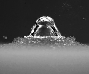
Figure 7. Final phase of the bubble collapse near the different granular boundaries at  $\gamma \approx 0.8$: (a) coarse sand ( $d_g=350\,\mathrm {\mu }{\rm m}$), (b) medium sand ( $d_g=200\,\mathrm {\mu }{\rm m}$) and (c) fine sand ( $d_g=90\,\mathrm {\mu }{\rm m}$). All image sequences are initiated 0.77 ms after the bubble generation and the time interval between successive images is 15 $\mathrm {\mu }$s. The white line indicates the 2 mm scale.
During the bubble growth phase (figure 6, frame 1–3), the granular beds undergo a weak local compaction, and the sand particles are slightly pushed radially outwards. This motion strictly follows the bubble dynamics and can therefore be attributed to the pressure and velocity fields generated by the expanding bubble. Although all sand sizes appear to follow a similar motion, the granularity of the nearby sand beds impacts the bubble growth differently. While the coarse sand allows the bubble to maintain an almost spherical shape, the finer sand forces the bubble's lower hemisphere to flatten. The former dynamics suggests the liquid is allowed to flow through the granular medium whereas the latter dynamics resemble the one imposed by a rigid, impermeable boundary. Consequently, one can deduce a direct relation between sand grain size and the permeability of the granular interface. To support this hypothesis, we turn to the well-established Ergun correlation (Ergun Reference Ergun1952) that evaluates the pressure drop,  $\Delta P$, of a steady-state fluid flow across porous media of length $L$,
$L$,
 \begin{equation} \frac{\Delta P}{L} = A \frac{\mu (1-\beta)^2 v_s}{d^2\beta^3} + B\frac{\rho (1-\beta) v_s^2}{d\beta^3}, \end{equation}
where  $\beta$ is the porosity of the medium, $d$ the mean sand grain diameter, $\mu$ and $\rho$ are the fluid dynamics viscosity and density, respectively, and $v_s$ is the superficial velocity. The constants $A$ and $B$ are determined empirically and have been a subject of debate (Macdonald et al. Reference Macdonald, El-Sayed, Mow and Dullien1979; Foumeny et al. Reference Foumeny, Benyahia, Castro, Moallemi and Roshani1993; Nemec & Levec Reference Nemec and Levec2005). The first term on the right-hand side of (3.1) represents the viscous energy losses that primarily occur in laminar flows and the second term denotes the energy losses in turbulent flow regimes. Assuming that $v_s$ is mostly independent of the sand grain size since the flows are driven by identical bubbles, and given that we measured similar porosities $\beta$ for all three granular interfaces, (3.1) yields a pressure drop that scales as $\Delta P \sim d^{-2}$ in the laminar flow regime and as $\Delta P \sim d^{-1}$ in the turbulent flow regime. In either case, a finer grain size results in a larger flow resistance in a steady-state regime, which can be associated with a lower permeability and could explain the different bubble dynamics.
After reaching a maximum radius (figure 6, frame 3), the bubble collapses (figure 6, frames 4–7). The previously radially displaced sand is now attracted by the retreating bubble and eventually forms a mound whose size depends on the sand granularity. The coarse sand scarcely forms a mound and the bubble simply becomes elongated in a direction perpendicular to the granular bottom (figure 7a, frames 1–4). The lower hemisphere flattens slightly due to the presence of the nearby sand bottom. The upper hemisphere maintains a spherical shape until the very last instants of the bubble collapse when it gently and gradually indents. This eventually results in the formation of a micro-jet that strikes the opposite side of the bubble at an average speed of approximately 218  ${\rm m}\,{\rm s}^{-1}$ (figure 7a, frame 5), whereupon the remaining torus collapses (figure 7a, frame 6). Close to the medium and fine sands, the collapse dynamics differ. The bubble's lower hemisphere flattens rapidly, and the sand is drawn toward the retreating bubble, leaving a thin film of fluid between the bubble and the sand interface (figure 6b,c, frames 6). Due to the proximity of the bubble to the granular interface, the fluid flow beneath the bubble is hindered. As a result, its upper hemisphere collapses faster, leading to the formation of a cone-shaped bubble (figure 7b,c, frames 1–3). Subsequently, a high-velocity micro-jet directed toward the boundary is formed (figure 7b,c, frame 4). This micro-jet reaches an average speed of 289 ${\rm m}\,{\rm s}^{-1}$ for a bubble near the medium sand and 328 ${\rm m}\,{\rm s}^{-1}$ for a bubble near the fine sand. As a comparison, a similar bubble evolving near a rigid boundary develops an average jet speed of 87 ${\rm m}\,{\rm s}^{-1}$. The aforementioned micro-jet velocities are evaluated by tracking the position of the jet tip as it moves through the bubble, taking into account the optical refraction at the bubble surface using Snell's law (Koch et al. Reference Koch, Rosselló, Lechner, Lauterborn, Eisener and Mettin2021). Depending on the velocity of the jet and the visibility of the bubble interior, at least 15 consecutive points can be collected from the 5 millions frames s $^{-1}$ recording. We find a near-linear evolution of the micro-jet tip position with time and, therefore, evaluate the averaged jet velocity by fitting a linear regression to our measurements. Note that we can only track the positions of the micro-jet in the upper hemisphere of the bubble, since the reflection of the granular interface on its lower hemisphere masks the jet. The difference in micro-jet velocity can be explained by the shape that the bubble assumes before its upper hemisphere indents. In the case of a bubble interacting with the fine or medium sand, the contraction of its lateral sides is significantly greater than it is for a bubble close to the coarse sand (figure 7, frames 2–3). The upper hemisphere of the bubble therefore exhibits a greater curvature before indentation which, in turn, yields thinner and faster micro-jets, as illustrated in figure 8(e). The size of the bubble at jet impact is also illustrated in figure 8. Bubbles interacting with a finer sand exhibit a larger volume at jet impact. This is because the height of the sand mound depends on the sand granularity: a finer sand yields higher mounds. Consequently, the bubble near a finer sand becomes locally closer to the granular interface which causes the jet to form earlier in the collapse phase, similar to the case of bubbles that are initiated nearer and nearer to a rigid boundary (Lechner et al. Reference Lechner, Lauterborn, Koch and Mettin2020). Before proceeding further, we should mention that bubbles generated at $\gamma > 1$ near the fine and medium sands do not develop a conical shape, but simply elongate in a direction perpendicular to the granular boundary. This is probably because the distance between the collapsing bubble and the sand mound is too great to sufficiently impede the fluid flow beneath the bubble.

Figure 8. Observation of the micro-jets driven by the nearby boundaries at  $\gamma \approx 0.8$: (a) fine sand ( $d_g=90\,\mathrm {\mu }{\rm m}$), (b) medium sand ( $d_g=200\,\mathrm {\mu }{\rm m}$), (c) coarse sand ( $d_g=350\,\mathrm {\mu }{\rm m}$) and (d) rigid boundary. The white line indicates the 2 mm scale. (e) The associated averaged jet speeds measured between jet formation and opposite bubble wall impact, and the curvatures of the bubbles upper hemispheres measured before the micro-jet formation.
After the collapse, the difference between the bubble dynamics close to a granular boundary and a rigid boundary is still striking (figure 6, frames 8–12). Near a rigid surface, the bubble rebound stretches over the boundary. However, when the bubble hits a granular interface, the sand ‘swallows’ the bubble, which then bounces back within the porous medium. This rebound is evidenced by the shock waves generated when the bubble collapses a second time. Following the first collapse of the bubble, the coarse sand is explosively ejected in random directions, pushed away radially by the rebound of the bubble. The fine sand, on the other hand, shows a completely different behaviour. The mound that had previously formed settles slowly, in a fluid-like cohesive fashion, suggesting that the bubble rebound is cushioned by the sand. The medium sand behaves in an intermediate manner: the upper layer of sand is thrown upward, again probably due to bubble rebound, but the lower layers begin to settle similarly to the fine sand. The difference in behaviour can be explained by the relative position of the bubble to the boundary. As a bubble evolves close to the coarse granular boundary, the sand is barely lifted. Therefore, the distance between the collapsing bubble and the sand is kept large enough so that, during the first phase of the rebound, the bubble is not entirely ‘swallowed’ by the sand. However, the mounding of the medium and fine sands forces the bubble to collapse closer to the granular interfaces. Consequently, the rebounding bubble is almost immediately ‘swallowed’ by the granular media, resulting in a less violent rebound and less pronounced ejection of sand grains. This reasoning is supported by the duration of the bubble's second oscillation period. We indeed measured a significantly longer second oscillation period for the bubble evolving close to the coarser sand, thus suggesting a larger and more energetic rebound.
3.1.3. Bubble-sand interaction at small stand-off distances: $\gamma \approx 0.6$ – $\gamma \approx 0.3$


Further reducing the stand-off distance leads to stronger bubble-sand interactions. To illustrate this behaviour, we show in figures 9 and 10 the dynamics of a bubble evolving at  $\gamma \approx 0.5$ from the considered interfaces. Figure 9 provides an overview of the bubble's lifetime and figure 10 shows the final instants of its first collapse.

Figure 9. Selected instants of the bubble dynamics near the different investigated boundaries at  $\gamma \approx 0.5$: (a) coarse sand ( $d_g=350\,\mathrm {\mu }{\rm m}$), (b) medium sand ( $d_g=200\,\mathrm {\mu }{\rm m}$), (c) fine sand ( $d_g=90\,\mathrm {\mu }{\rm m}$) and (d) rigid boundary. Image sequences are initiated between 0.05 and 0.06 ms after the bubble generation and the time interval between successive images is 0.1 ms. The 0.01 ms jitter between the onset of the image sequences was chosen so that the first collapse of the bubble and the shock wave emission occurs for all three granular boundaries on frame 9 and, for the rigid boundary, on frame 10. This offset corresponds to approximately 1.2 % of the bubble first oscillation period. The white line indicates the 2 mm scale.

Figure 10. Final phase of the bubble collapse near the different granular boundaries at  $\gamma \approx 0.5$: (a) coarse sand ( $d_g=350\,\mathrm {\mu }{\rm m}$), (b) medium sand ( $d_g=200\,\mathrm {\mu }{\rm m}$) and (c) fine sand ( $d_g=90\,\mathrm {\mu }{\rm m}$). All image sequences are initiated 0.76 ms after the bubble generation and the time interval between successive images is 20 $\mathrm {\mu }$s. The white line indicates the 2 mm scale.
Near the granular boundaries, the bubble sticks to the boundary early in its growth phase and initially maintains a spherical shape, in contrast to the bubble near the rigid interface, whose lower hemisphere quickly flattens (figure 9, frame 1–2). As discussed in § 3.1.2, this difference of dynamics suggests that the part of the liquid displaced by the bubble can flow through the permeable granular medium, allowing the bubble to retain a higher symmetry. As the bubble continues to grow (figure 9, frames 2–5), the sand is first compacted downwards and is then pushed radially outwards. This combined motion of the granular media leads to the formation of a crater in which the bubble evolves. The shape and size of the crater is nevertheless highly dependent upon the sand grain size. The fine and medium sand deform greatly, leading to the formation of a notable rim encircling the bubble towards the end of its growth and during its collapse phase. The coarse sand, on the other hand, is weakly displaced, resulting in a significantly less pronounced crater rim (figure 10, frames 1–4). The formation of a crater also likely allows the lower hemisphere of the bubble to continue to grow downwards while preventing it from stretching along the granular boundary, in contrast to a bubble near a rigid boundary that expands along the solid wall and assumes a hemispherical shape. These differences in the growth phase ultimately affect the collapse of the bubble.
During the collapse phase (figure 9, frames 5–9) the presence of the granular boundary impedes the liquid flow below the bubble. This leads to the delay of the lower hemisphere collapse with respect to the upper one. For the coarse sand, the resulting effect is similar to the one observed at  $\gamma \approx 0.8$: a faster contraction of the bubble's lateral sides (figure 9a, frame 8) followed by a gradual collapse of the upper hemisphere (figure 10a, frames 1–4) that eventually indents, resulting in the formation of a micro-jet impacting the bubble's opposite wall (figure 10a, frames 5–6). A local measurement of the jet velocity yields a speed of approximately 227 ${\rm m}\,{\rm s}^{-1}$, considering the optical refraction at the bubble interface. In contrast, for the medium and fine sands, the formation of a larger rim surrounding the bubble leads to a drastically different collapse. The bubble's surface indentation is now visible on its lateral sides (figure 9b,c, frames 7–8). This is likely the result of an annular flow converging toward the bubble's axis of symmetry. As the bubble continues to collapse, it develops a bell-shaped form with a spherical cap, an annular indentation and a conical flank (figure 10b,c, frames 1–3). The cap's lateral sides collapse first suggesting the annular flow is faster than the axial flow. When the annular flow collides, a shock wave is emitted in the liquid phase and a fast micro-jet is accelerated downwards, as illustrated in figure 11. Considering the micro-jet is initiated upon the liquid collision (Reuter & Ohl Reference Reuter and Ohl2021), we estimate its velocity by measuring the distance travelled by the jet between its initiation (i.e. cap collapse) and the location at which the jet tip goes past the granular rim, still considering the optical refraction at the bubble interface. Particularly high jet velocities are measured that range between 1083 ${\rm m}\,{\rm s}^{-1}$ and 1138 ${\rm m}\,{\rm s}^{-1}$. Resembling dynamics with similarly fast micro-jets have already been described for bubbles that collapse extremely close to a solid boundary. Lechner et al. (Reference Lechner, Lauterborn, Koch and Mettin2019, Reference Lechner, Lauterborn, Koch and Mettin2020) computed jet velocities ranging between 1000 ${\rm m}\,{\rm s}^{-1}$ and 2000 ${\rm m}\,{\rm s}^{-1}$ depending on the stand-off distance ( $\gamma =0.05-0.2$), Koch et al. (Reference Koch, Rosselló, Lechner, Lauterborn, Eisener and Mettin2021) successfully compared the micro-jet dynamics of a laser-induced bubble at $\gamma = 0.04$ with a ray-traced numerical simulation, which yielded a fast micro-jet velocity of over 700 ${\rm m}\,{\rm s}^{-1}$, and Reuter & Ohl (Reference Reuter and Ohl2021) measured a lower bound on the jet velocity of 850 ${\rm m}\,{\rm s}^{-1}$ for a bubble collapsing at a stand-off distance $\gamma =0.05$. It is not clear why a bubble generated at a distance $\gamma \approx 0.5$ close to a bed of sand develops similar dynamics. However, a possible explanation could be found in the elevation of the granular boundary, since its upward displacement causes a local change of the stand-off distance that could lead to the bubble dynamics mentioned above. Before moving forward, we should mention that a bubble generated over the coarse sand exhibits the same bell-shaped profile at $\gamma \approx 0.3$, while the one developing over the fine sand adopts these dynamics at $\gamma \approx 0.6$ already. This behaviour is consistent with the premise that the finer the sand grains, the larger the interface deformation, and, thus, the stronger its impact on the bubble dynamics. After collapsing, the bubble is ‘swallowed’ by the sand inside which it rebounds. Again, the presence of the rebound is confirmed by the shock waves emitted when the bubble collapses a second time. Immediately after collapse (figure 9, frames 9–12), the sand grains are gradually lifted. The extent and cohesion of this movement depends on the grain size. While the finer sand shows a slow but cohesive upward movement, the coarser sand rises rapidly in a scattered manner. The difference in dynamics could be explained by the amplitude of the bubble rebound. We indeed measure that the bubble rebound in the coarser sand lasts longer than the one in the finer sand, implying a more energetic rebound that can propel the sand particles farther away.

Figure 11. Snapshots of the shock waves emitted upon cap collapse (a,b) and resulting micro-jets (c,d) for the medium sand (a,c) and fine sands (b,d) at  $\gamma \approx 0.5$. All images were taken 1.2 $\mathrm {\mu }$s after the cap collapse. The white line indicates the 2 mm scale.
Following the bubble collapse, the sand motion continues on a much longer time scale (several tens of milliseconds, compared with the bubble lifetime of approximately 1 ms). To illustrate this motion, we show in figure 12, the dynamics of the sand induced by a bubble collapsing at  $\gamma \approx 0.6$ for all three grain sizes. In all three cases, the sand motion is driven by a bubble with a maximum radius $R_{max} \approx 4.44$ mm. The first frame in figure 12 is taken 1 ms after the bubble generation. To put these images in a temporal context, it should be noted that the bubble's first oscillation period lasts approximately 860 $\mathrm {\mu }$s and its second oscillation period lasts between 380 $\mathrm {\mu }$s and 560 $\mathrm {\mu }$s, depending on the grain size (a larger grain size leads to a longer rebound at $\gamma \approx 0.6$). This means that the bubble has already collapsed once after 1 ms and is rebounding within the sand. The occurrence of the bubble rebound below the sand surface is confirmed by the presence of shock waves emitted during its second collapse, as illustrated in figure 13. The dashed line in 12 frame 1 indicates the height of the sand mound at the time of the bubble's first collapse. As illustrated in frame 1, all three mounds have risen from this position. The dynamics of the coarse sand continues as follows. The sand grains ejected from the rebounding bubble are propelled further (frames 2–3). As these particles slow down, a granular jet can be observed shooting upwards in the centre of the ejecta (frames 4–5). The jet eventually reaches a maximum height and the sand grains rain down to the ground (frame 6). The fine sand dynamics also exhibit a jetting behaviour, but, its dynamics differ from the one described above. Immediately after the bubble collapse, the mound, which had risen slightly (frame 1), collapses radially back inwards (frame 2). This is followed by the formation of a thin jet that migrates away from the boundary and forms a vortex ring (frame 3–5). After reaching a maximum height the collimated thin jet disperses and the sand grains fall back onto the granular surface (frame 6). The medium sand exhibits an intermediate behaviour between the coarse and fine sands. The velocity and height of the jets depend on the grain size. While the fine sand jet quickly reaches a considerable height of 15.2 mm in 60 ms, the coarse sand reaches 9.7 mm after 60 ms and the medium sand 10.8 mm after 60 ms. Both the medium and fine sand jets reach heights beyond the available field of view (15.8 mm). The coarse sand jet only reaches a height of approximately 10.1 mm.

Figure 12. Granular jet dynamics following the bubble collapse. The bubble driving the jets is generated at  $\gamma \approx 0.6$ and has a maximum radius $R_{max} \approx 4.44$ mm. (a) Coarse sand ( $d_g=350\,\mathrm {\mu }{\rm m}$), (b) medium sand ( $d_g=200\,\mathrm {\mu }{\rm m}$) and (c) fine sand ( $d_g=90\,\mathrm {\mu }{\rm m}$). The white dashed line indicates the elevation of the granular mounds at the bubble first collapse and the white solid line indicates the 3 mm scale.

Figure 13. Evidence of the bubble rebound below the sand surface from the shock waves emitted during its second collapse. The bubble is generated at  $\gamma \approx 0.6$ with $R_{max} \approx 4.44$ mm. (a) Coarse sand ( $d_g=350\,\mathrm {\mu }{\rm m}$) and (b) fine sand ( $d_g=90\,\mathrm {\mu }{\rm m}$). The associated bubble first oscillation period approximately lasts 0.86 ms for both the coarse and fine sands and the white solid line indicates the 2 mm scale.
Similar sand jets have already been observed in air when a solid sphere impacts and penetrates a bed of loose sand, leaving a cavity in its path (Thoroddsen & Shen Reference Thoroddsen and Shen2001; Lohse et al. Reference Lohse, Bergmann, Mikkelsen, Zeilstra, van der Meer, Versluis, van der Weele, van der Hoef and Kuipers2004; Royer et al. Reference Royer, Corwin, Flior, Cordero, Rivers, Eng and Jaeger2005; Caballero et al. Reference Caballero, Bergmann, van der Meer, Prosperetti and Lohse2007), or when a pressurised gas cavity explodes and collapses inside a bed of sand (Loranca-Ramos, Carrillo-Estrada & Pacheco-Vazquez Reference Loranca-Ramos, Carrillo-Estrada and Pacheco-Vazquez2015). In both cases, the jetting is attributed to the collapse under gravity of the cavity that is left within the sand. Therefore, we believe that the sand jets we observe could be attributed to a similar phenomenon taking place when the bubble bounces back below the sand surface. As the bubble rebounds, the sand would presumably be forced radially outwards, creating a cavity in the granular medium, and then converge radially back inward to fill the created void. The sand grains would eventually collide and form a jet that rises upwards. Alternatively, the jetting behaviour could also be attributed to the flow field induced by the collapse of the rebound bubble. This reasoning is derived from the work of Reuter et al. (Reference Reuter, Gonzalez-Avila, Mettin and Ohl2017) who have shown that when a bubble oscillates near a solid surface at  $0.5 \lesssim \gamma \lesssim 1.3$, large upward fluid displacements are produced by an ascending vortex ring that forms after the toroidal second collapse of the bubble. By tracking the fluid displacement caused by this bubble collapse, the authors identified very similar flow patterns to those observed here via the displacement of the medium and fine sand particles: a vortex ring gradually migrating away from the boundary. Both explanations have their merits, and the actual jet driving mechanism could be a combination of the two. A definitive answer would nonetheless be provided by investigating the dynamics of the bubble and sand particles under the granular surface using, for instance, high-speed X-ray radiography, as performed by Royer et al. (Reference Royer, Corwin, Flior, Cordero, Rivers, Eng and Jaeger2005) in the case of a sphere impacting a granular boundary.
Our observations suggest that the jetting phenomenon discussed above mainly occurs for  $\gamma \lesssim 1.3$, i.e. when the bubble's second collapse takes place below the sand bed. However, the detailed dynamics of these granular jets (velocity, height, width, etc.) appear to depend on all three parameters modulated in this study: bubble energy, grain size and the initial distance between the bubbles and the sand surface. A future study would therefore be needed to thoroughly correlate the bubble properties with their effects on the sand jets. At $\gamma \gtrsim 1.3$, the movement of the granular boundary is predominantly characterised by an upward ejection of the surface sand particles, likely due to a momentum transfer between the liquid flow, accelerated by the bubble dynamics, and the sand bed.
3.2. Analysis of key bubble dynamics parameters
In the following sections we present two key parameters of the bubble dynamics: the bubble oscillation periods and the displacement of its centroid. The presented data include the entire parameter space covered by the experiment, i.e. bubble energies and stand-off distances. The experimental data are compared against the simulation results obtained from the BIM.
3.2.1. Bubble oscillation periods
The bubble oscillation periods are an important characteristic of the bubble dynamics as they vary with both the stand-off distance and the nature of the nearby boundary. In figure 14 we show the evolution of the bubbles first and second oscillation periods as a function of the stand-off distance  $\gamma$ and the anisotropy parameter $\zeta$. For comparison, the results for bubbles developing near a rigid surface are also included. The bubbles first oscillation period, $t_{c1}$, is measured with the laser-beam deflection probe (see § 2.1). The second oscillation period, $t_{c2}$, is also mainly determined with the same probe. However, when a bubble is generated close to the granular boundary ( $\gamma \lesssim 1.0$), its second collapse takes place within the sand, resulting in a weaker emitted shock wave that the probe is unable to detect. Instead, the timing of the second collapse shock wave is visually determined through the high-speed recording (hollow markers in figure 14). The latter measurement is only conducted for the largest bubble energy. For the convenience of comparison, the collapse times are normalized by twice the Rayleigh collapse time of the unbounded bubble, $t_{c0} = 1.83R_{max}(\rho /\Delta p)^{0.5}$ (Rayleigh Reference Rayleigh1917). We also include in figure 14 the results of the BIM simulation. Overall, the general trends are well predicted by the numerical model, although the simulations slightly overestimate the collapse times for both the solid and sand boundaries test cases, with a root-mean-square error of 2.6 % for the sand boundary and of 3.8 % for the rigid boundary over the considered data range ( $1.0 < \gamma < 6.0$). These discrepancies could be attributed to effects of viscosity, surface tension or compressibility that are neglected in the simulations.

Figure 14. (a) Normalized first oscillation and (b) second oscillation periods of the bubbles as a function of the stand-off distance  $\gamma$. The solid symbols indicate the values estimated through the laser-beam deflection probe. The hollow symbols indicate the values visually estimated through high-speed recording by identifying the shock waves emitted upon collapse. (c) Second oscillation period as a function of $\zeta$.
As illustrated in figure 14(a), the presence of a granular boundary leads to a gradual increase of  $t_{c1}$ as the bubble is generated closer and closer to the interfaces. Interestingly, the grain size has no significant impact on the bubble lifetime within the measurement's uncertainties. Bubbles close to a rigid boundary follow a similar trend, but the prolongation of their first oscillation periods is significantly more pronounced. At large stand-off distances, the bubbles oscillation times approach that of the unbounded spherical bubbles, that is, $t_{c1}/t_{c0} \to 1$. In figure 14(b) we present the bubbles second oscillation periods as a function of $\gamma$. The results show that a decrease of the stand-off distance results in longer rebounds until a maximum is reached at $\gamma \approx 1.1$ for the granular interfaces and $\gamma \approx 1.3$ for a rigid boundary. As discussed in § 3.1.1, this lengthening can be explained by the increasing anisotropy of the pressure field, leading to weaker first collapses and, thus, more energetic and larger rebounds. The sand grain size has no significant impact on the bubbles’ second oscillation period for $\gamma \gtrsim 1.1$. At stand-off distances $\gamma _{sand} \lesssim 1.1$ and $\gamma _{rigid} \lesssim 1.3$, the rebound oscillation times decrease with $\gamma$. We believe this behaviour is due to the stronger physical interactions between the bubbles and the nearby boundaries, resulting in greater energy losses. We also find that the sand grain size affects the rebounding dynamics between $0.3 \gtrsim \gamma \lesssim 1.1$. Within this range of stand-off distances, the bubble is ‘swallowed’ by the granular boundary and consistently exhibits shorter second oscillation periods when it develops in sands with finer grain sizes.
Considering that the rebound dynamics is correlated to the anisotropy of the pressure field, we show in figure 14(c) the second oscillation periods of the bubbles as a function of the dimensionless anisotropy parameter  $\zeta$ (see (1.1)). For bubbles near a granular interface, we use the same assumptions as for the numerical model and consider the sand as a liquid whose density is defined by a mixture law. The anisotropy parameter is therefore given by $\zeta = 0.195(\rho _m-\rho _w ) (\rho _m+\rho _w )^{-1} \gamma ^{-2} \approx 0.0616\gamma ^{-2}$. Bubbles near a rigid surface are characterized by an anisotropy given by $\zeta = 0.195\gamma ^{-2}$. Considering the anisotropy parameter instead of the stand-off parameter, we find that the duration of the bubble rebounds strongly depends on the pressure field anisotropy and is almost independent of the anisotropy source (i.e. rigid or granular boundary) for $\zeta \lesssim 0.06$, which roughly corresponds to $\gamma _{sand} \approx 1.1$.
3.2.2. Bubble translation
Another important feature of the bubble dynamics is the displacement of its centroid, as the potentially damaging micro-jets and shock waves generated during collapse are closely related to the bubble migration. We present in figure 15 the bubble centroid translation,  $\Delta z$, as a function of the stand-off parameter $\gamma$ and the dimensionless anisotropy parameter $\zeta$, for all the investigated sand granularities and bubble energies. The centroid displacement is defined as the distance travelled by the bubble centre of mass between its generation and collapse, which is taken as the moment when the bubble reaches its minimum volume. We normalize the displacement by the unbounded bubble maximum radius, $\Delta z/R_{max}$, so that different bubbles can be compared. The solid symbols in figure 15 indicate the displacement measured through the camera recordings. As $\gamma$ is decreased below 0.6, however, the uplifting of the sand bottom masks the final instants of the bubble collapse and prevents an accurate assessment of its location. Instead, we fit circles to the shock waves emitted upon the bubble collapse to estimate its location. These results are indicated by hollow symbols in figure 15. The latter measurement was only conducted for the largest bubble energy. In addition, figure 15(a) shows the data computed with the BIM. The results show a good agreement with the experimental data. Over the range of simulated data ( $1.0 < \gamma < 6.0$), the root-mean-square error of the bubbles migration predictions is roughly 6.1 % for both the granular and the solid boundary. The discrepancies between the numerical and experimental data are more pronounced at large values of $\gamma$. This is because the limited temporal and spatial resolution of the high-speed recording makes it difficult to accurately determine the position of the bubble when it reaches a minimum volume at large stand-off distances. Overall, the migration trends are well estimated by the simple and efficient numerical method.

Figure 15. Normalized bubble centroid displacement from generation to the first collapse as a function of the stand-off parameter  $\gamma$ (a) and anisotropy parameter $\zeta$ (b). The solid symbols indicate values estimated through the high-speed camera recording, the hollow symbols indicate the displacements found by fitting circles to the shock waves emitted upon collapse to estimate the collapse location.
As shown in figure 15(a), the bubble migration near a granular boundary at large stand-off distances is barely notable and approaches that of an unbounded spherical bubble,  $\Delta z/R_{max} \to 0$. As the stand-off distance is decreased, we observe an increase of the bubble migration that is independent of the bubble energy and the sand granularity. This trend is due to a gradual increase of the pressure field anisotropy and continues until $\gamma \approx 0.6$ where the presence of the near boundary prevents any further bubble displacement and $\Delta z /R_{max}$ decreases. A comparison with the solid boundary shows that the bubbles undergo a similar trend. The magnitude of the displacement is nonetheless significantly higher for bubbles near a rigid boundary. The difference in the magnitude of the displacement between bubbles near the sand and a rigid boundary is explained by the weaker anisotropy in the pressure field caused by the granular boundary. To further exploit the dependance of the bubble migration on the flow field anisotropy, we show in figure 15(b) the bubble translation as a function of $\zeta$, using the flat rigid boundary definition for the solid boundary and the liquid–liquid boundary definition for the granular boundary (see (1.1)). This procedure leads to a near overlap of the displacement curves and illustrates the independence of the bubble translation from the anisotropy source (i.e. rigid or granular boundary) for anisotropy numbers up to $\zeta \approx 0.08$. This limit agrees well with the work of Supponen et al. (Reference Supponen, Obreschkow, Tinguely, Kobel, Dorsaz and Farhat2016), who showed that important parameters of the bubble dynamics, such as micro-jets physics and bubble displacements, were independent of the anisotropy source for $\zeta < 0.1$. These authors additionally derived a power law to predict the normalized displacement of the bubble centroid, $\Delta z /R_{max}=2.5\zeta ^{3/5}$. Their choice of the exponent is based on the premise that, in a scale-free framework, all lengths scale proportionally to the characteristic bubble radius at the final collapse stage, $r\equiv R(t)/R_{max}$, which itself scales as $r \sim \zeta ^{2/3}$ (a thorough explanation of this derivation can be found in Supponen et al. Reference Supponen, Obreschkow, Tinguely, Kobel, Dorsaz and Farhat2016). Hence, the bubble displacement scales as $\Delta z \sim r \sim \zeta ^{2/3}=\zeta ^{0.667}$ when the centroid motion uniquely occurs at the final collapse stage. However, to account for the fact that part of the bubble migration takes place before the final collapse instants, the authors corrected this scaling to $\Delta z \sim \zeta ^{3/5}=\zeta ^{0.6}$. As illustrated in figure 15(b), we however find that the power law $\Delta z /R_{max}=2.5 \zeta ^{2/3}$ fits our experimental data well, without the need for a correction to the exponent. We believe this difference can be explained by the choice of definition for the bubble centroid at collapse. While Supponen et al. (Reference Supponen, Obreschkow, Tinguely, Kobel, Dorsaz and Farhat2016) defined the centroid position at collapse as the position of the micro-jet tip at impact with the opposite bubble wall, we consider the centre of mass of the bubble when it reaches its minimum volume. Our definition leads to smaller bubble displacements, which is consistent with our choice of exponent for $\zeta < 0.1$. We also note that our definition of $R_{max}$ for normalization may lead to slight discrepancies compared with the results of Supponen et al. (Reference Supponen, Obreschkow, Tinguely, Kobel, Dorsaz and Farhat2016), as the authors considered the maximum bubble radius and we consider the maximum unbounded bubble radius. Nonetheless, at $\zeta \approx 0.08$ (i.e. $\gamma _{sand} \approx 0.9$ and $\gamma _{rigid} \approx 1.6$), we estimated this difference to be of the order of 2-4 % (see § 2.1).
4. Conclusion
This study focused on the dynamics of laser-induced cavitation bubbles near beds of sand composed of spherical soda lime glass beads. We considered three different sand grain sizes and performed high-speed visualisations of the bubbles and sands dynamics, varying the stand-off distance between  $\gamma \approx 0.3$ and $\gamma \approx 5.3$.
The observed bubble behaviour can be divided into three regimes associated with specific ranges of stand-off parameter. For  $1.3 \lesssim \gamma \lesssim 5.3$, the sand grain size has a weak influence on the bubble dynamics which resemble that of a similar bubble developing over a rigid boundary. At intermediate stand-off distances, between $\gamma \approx 1.3$ and $\gamma \approx 0.6$, the sand is lifted during the bubble collapse and eventually forms a mound, whose size depends upon the distance of the bubble to the sand and its granularity. The bubble rebound is ‘swallowed’ by the sand. At small stand-off distances, below $\gamma \approx 0.6$, the bubble develops a bell-shaped form as it collapses, resulting in the formation of a thin and very fast micro-jet. The sand granularity dictates the minimum stand-off distance where this behaviour is observable. In this regime, the bubble is ‘swallowed’ by the sand in the last instants of its first collapse. Compared with a rigid boundary, we found that the bubble lifetime is shortened with a reduced centroid displacement for all tested $\gamma$ values. Between $\gamma \approx 1.3$ and $\gamma \approx 0.3$, we additionally observed granular jets erupting from the sand surface after the bubble has collapsed.
Defining the sand as an equivalent liquid with a mixture law, we found that the dimensionless anisotropy parameter  $\zeta$ could be used to predict the bubble centroid displacement with a scaling law for $\zeta \lesssim 0.08$. The use of the anisotropy parameter also proved to be a particularly suitable means of comparing the duration of the bubbles first rebound between a rigid surface and a granular interface for $\zeta \lesssim 0.06$.
Moreover, we developed a numerical model based on the BIM to predict and explain the bubble dynamics close to a granular boundary. The BIM simulations successfully reproduce the bubbles behaviour in the range of stand-off distances where the bubble dynamics is largely independent of the sand grain size, i.e. for  $\gamma \gtrsim 1.3$.
The presented results might be useful in the field of underwater explosions, especially when the charges are detonated near the sandy bottom. In addition to such an application, this study also presents a compelling scientific interest that remains largely unexplored and will hopefully pave the way for future interest and research in the area. For example, the dynamics of a cavitation bubble in a granular medium could be further examined to gain a better understanding of the mechanisms involved in ultrasonic deagglomeration/dispersion, where the interactions of the bubbles with the particles could be important.
Funding
We gratefully acknowledge the support of the Swiss National Science Foundation (grant no. 179018) and the MSCA-ITN-ETN of the European Union's H2020 program (REA grant agreement no. 813766).
Declaration of interests
The authors report no conflict of interest.
Appendix. Boundary integral method and experiments comparison
Figure 16(a) shows a comparison of the bubble profiles between the experimental observations (left halves of the frames) and the BIM simulation (right halves of the frames) for a stand-off distance  $\gamma = 1.27$ near the medium sand. It should be noted that the simulation profiles are two-dimensional cross-sections of the bubble along its axis of symmetry, while the experimental profiles are shadowgraphs obtained with backlighting. The spatiotemporal evolution of the bubble motion is closely reproduced by the BIM between frames 1 and 5 (growth phase). Nonetheless, the simulation slightly overestimates the bubble maximum radius and, since the bubble oscillation period is proportional to the maximum radius, the collapse is delayed with respect to the experimental observations. We measured this delay to be 29 $\mathrm {\mu }$s, which roughly corresponds to a relative error of 3.5 % with respect to the experiment. Therefore, to compare the bubble profiles during the collapse phase, we shifted the times of the numerical simulation by 29 $\mathrm {\mu }$s on frames 6–9 (right halves). With this temporal correction the bubble profile is also well reproduced over the collapse phase. However, we note that the extent of the lower hemisphere of the bubble is overestimated in the simulation, likely due to the overestimation of the downward sand displacement. Immediately before the micro-jet hits the opposite bubble wall (frame 9), the simulation results show a bubble shape and position that agree remarkably well with the experimental observations. To further illustrate the independence of the bubble dynamics from the sand grain size at $\gamma \gtrsim 1.3$, we also show in figure 16(a) the profiles of the bubble near the coarse and fine sands before micro-jet impact, and compare them with the BIM. Performing a similar temporal correction, the simulation results are found to nearly overlap the experimental observations. Figure 16(b) shows the time evolution of the equivalent bubble radii for both the BIM simulations and the experimental observations. We find a close agreement between the obtained radii, but notice a small temporal shift, which we explain by the delayed bubble collapse in the simulation. In figure 16(c) we show the temporal evolution of the bubble centre of gravity. The overall agreement is good, although the simulation predicts the bubble centroid closer to the boundaries than in the experiments.

Figure 16. Comparison of bubble dynamics between BIM and experiments at a stand-off distance  $\gamma =1.27$. (a) Growth and collapse of a bubble in the vicinity of the medium sand: experiment (left) and BIM (right). The dimensional times of the numerical simulation are: 0.01, 0.11, 0.21, 0.32, 0.42, 0.56, 0. 66, 0.76, 0. 87 (in ms). The final instants of a bubble evolving close to the coarse sand (simulation time 0.86 ms) and the fine sand (simulation time 0.87 ms) are also included. The black line indicates the 2 mm scale. (b) The time evolution of the equivalent bubble radius and (c) the centroid displacement are compared with the BIM results. The experimental bubbles are generated at $z \approx 5.64$ mm above the boundaries and their maximum radius is $R_{max} \approx 4.44$ mm.
Considering the complexity of the simulated bubble dynamics problem and the simplicity and computational efficiency of the numerical model, we believe that the consistency between the numerical and experimental results is remarkably good.


 Open access