


1. Introduction
Hydrodynamic interactions between particles of approximately spherical shape are of great importance for many areas in research and industry, including colloid dynamics (Rex & Löwen Reference Rex and Löwen2008), polymers (Kirkwood & Riseman Reference Kirkwood and Riseman1948), deposition processes (Dabros Reference Dabros1989), and active systems such as microswimmers (Najafi & Golestanian Reference Najafi and Golestanian2004; Ishikawa, Simmonds & Pedley Reference Ishikawa, Simmonds and Pedley2006; Pooley, Alexander & Yeomans Reference Pooley, Alexander and Yeomans2007; Pande & Smith Reference Pande and Smith2015; Ziegler et al. Reference Ziegler, Scheel, Hubert, Harting and Smith2021) and Janus particles (Sharifi-Mood, Mozaffari & Córdova-Figueroa Reference Sharifi-Mood, Mozaffari and Córdova-Figueroa2016). Due to the small length scales involved, the corresponding hydrodynamic flows are dominated by viscous friction rather than by fluid inertia. In this regime, the Navier–Stokes equations reduce to the Stokes equations, which can be solved analytically at spatially constant viscosity for many geometries. Since viscosity gradients are abundant in both living and non-living environments, such as bacterial biofilms (Wilking et al. Reference Wilking, Angelini, Seminara, Brenner and Weitz2011), mucus layers (Swidsinski et al. Reference Swidsinski, Sydora, Doerffel, Loening-Baucke, Vaneechoutte, Lupicki, Scholze, Lochs and Dieleman2007) and interfaces between fluids of different viscosities (Qiu & Mao Reference Qiu and Mao2011), it is natural to ask how the hydrodynamic interactions change in viscosity gradients. In physical systems, such viscosity gradients can e.g. arise as a consequence of the viscosity's dependence on temperature (Oppenheimer, Navardi & Stone Reference Oppenheimer, Navardi and Stone2016), shear rate (Wells & Merrill Reference Wells and Merrill1961) or solvent concentration (Goldsack & Franchetto Reference Goldsack and Franchetto1977). The simplest example of such an environment is a linear viscosity gradient, i.e. a region in the fluid where the viscosity changes linearly with the position in space. Another experimentally relevant example is the viscosity perturbation induced by temperature contrasts between the interacting particles and the surrounding fluid (Kroy, Chakraborty & Cichos Reference Kroy, Chakraborty and Cichos2016; Oppenheimer et al. Reference Oppenheimer, Navardi and Stone2016). In both cases, results have already been obtained for the mobilities of single particles (Datt & Elfring Reference Datt and Elfring2019; Oppenheimer et al. Reference Oppenheimer, Navardi and Stone2016), while only little is known for the interaction between several particles.
In their seminal paper on microswimmer behaviour in a viscosity gradient, Liebchen et al. (Reference Liebchen, Monderkamp, Ten Hagen and Löwen2018) estimated an upper bound for the amplitude of the leading-order correction for the Oseen tensor within an infinite linear viscosity gradient, but neglected those terms in their subsequent analysis of swimmer behaviour in a viscosity gradient. Subsequently, Laumann & Zimmermann (Reference Laumann and Zimmermann2019) calculated the first-order correction to the Oseen tensor in an infinitely large linear viscosity gradient . However, to the best of our knowledge, no explicit results are yet available in the literature for the corrections to the full mobility matrix of two particles in non-homogeneous environments. Also, the studies mentioned did assume viscosity gradients that extend infinitely, although inevitably this introduces negative viscosity in some parts of the fluid. To avoid this, we consider explicitly viscosity gradients that, while being larger than the separation between both particles by at least an order of magnitude, are yet of finite size, and thus avoid negative fluid viscosity. For the second application of particles with a temperature difference with respect to the surrounding fluid, no results are yet available for the interactions between particles.
We fill this gap, providing the leading-order correction to the mobility matrix associated with the interaction of particles at large separations for both a large viscosity gradient as well as for viscosity perturbations due to the particle temperature. In the former case, we find, surprisingly, that the correction terms, which are to leading order linear in the viscosity gradient, scale constant in the distance between both particles. This is in contrast to the Oseen tensor, which decays with the first power of the inverse distance. For a particle subject to a torque, the correction to the flow field is scaling with the first power of the inverse distance to the particle, while the constant viscosity flow scales with the second power. Also, we discover that asymmetric particle placement in an odd symmetric viscosity gradient or an asymmetry in the domain of the viscosity gradient introduce an additional mobility term. This term has a non-negligible impact on both the self-mobility as well as the interaction between the two particles.
For particles with a temperature difference with the surrounding fluid, we find that the presence of a second hot or cold particle changes the self-mobility of the first particle. The effect is proportional to the inverse particle separation. The mobility term associated with hydrodynamic interaction between the particles is altered proportional to the second power of the inverse distance.
The paper is structured as follows. First, we introduce the problem of calculating the mobility matrix in non-constant viscosity in § 2, before we give a short derivation of the perturbative first-order correction to the mobility matrix following Oppenheimer et al. (Reference Oppenheimer, Navardi and Stone2016) (§ 3). We then employ a reflection method in order to expand the correction in the inverse separation of both particles, deferring the explicit calculation of the first-order terms to the Appendix. In § 4, we present results for two particles in a linear viscosity gradient of finite size, where we focus first on symmetric placement of particles in the gradient (§ 4.1), and second describe the additional terms arising when the particles are placed asymmetrically in the gradient (§ 4.2). As a second application, we focus on the mobility of a two-particle system with a temperature contrast between the particles and the fluid at infinity (§ 5). Section 6 concludes the paper. We also provide a list of symbols in table 1.
Table 1. List of symbols.

2. Formulation of the problem
We aim to calculate the mobility matrix for two spherical particles of equal radius  $a$ with relative distance $s$ between the centres of both particles, which are suspended in a fluid with position-dependent viscosity $\eta (\boldsymbol {r})$. We assume that the fluid viscosity is given by
 \begin{equation} \eta(\boldsymbol{r}) = \eta^{(0)} + \epsilon\,\eta^{(1)}(\boldsymbol{r}), \end{equation}
where  $\eta ^{(0)}$ is the reference viscosity, $\epsilon < 1$ is the perturbation parameter, and $\boldsymbol {r}$ is the position in the fluid. Upper indices in brackets correspond to orders in $\epsilon$. We assume that the viscosity perturbation is at most of the order of $\eta ^{(0)}$, such that $\epsilon$ corresponds to the ratio of the magnitudes of viscosity perturbation and the constant-viscosity background. The Reynolds number (Purcell Reference Purcell1977) associated with the particles is assumed to be zero, such that the fluid is described by the incompressible Stokes equations (Kim & Karilla Reference Kim and Karilla2005, p. 9)
 \begin{equation} \boldsymbol{\nabla} \boldsymbol{\cdot} \boldsymbol{\sigma} (\boldsymbol{r}) = 0, \quad \boldsymbol{\nabla} \boldsymbol{\cdot} \boldsymbol{u} (\boldsymbol{r}) = 0. \end{equation}
Here,  $\boldsymbol {u} (\boldsymbol {r})$ denotes the fluid velocity, $\boldsymbol {\sigma } (\boldsymbol {r})$ is the stress tensor defined as
 \begin{equation} \boldsymbol{\sigma} (\boldsymbol{r}) ={-} p(\boldsymbol{r})\,{\boldsymbol{\mathsf{I}}} + 2\,\eta(\boldsymbol{r})\, {\boldsymbol{\mathsf{E}}} (\boldsymbol{r}), \end{equation}
and the bold centred dot denotes contraction of the last index of the preceding quantity with the first index of the following quantity, as scalar products of vectors and matrix–vector products. Also,  $p (\boldsymbol {r})$ denotes the pressure in the fluid, ${\boldsymbol{\mathsf{E}}}(\boldsymbol {r}) = (\boldsymbol {\nabla } \boldsymbol {u} (\boldsymbol {r}) + (\boldsymbol {\nabla } \boldsymbol {u}(\boldsymbol {r}))^{\rm T} )$/2 is the strain rate in the fluid, and ${\boldsymbol{\mathsf{I}}}$ is the $3 \times 3$ identity matrix. The symbol T denotes matrix transposition.
Due to the linearity of the Stokes equations, there exists a linear relation between the (angular) velocities ( $\boldsymbol {U}_b$ and $\boldsymbol {\varOmega }_b$) of each particle and the hydrodynamic forces/torques ( $\boldsymbol {F}^{hydro}_b$ and $\boldsymbol {T}^{hydro}_b$) that the fluid exerts on each particle $b = 1, 2$. To shorten notation for the subsequent calculations, we introduce generalised velocity and force vectors:
 \begin{equation} \boldsymbol{\mathcal{U}} = (\boldsymbol{U}_1, \boldsymbol{U}_2, \boldsymbol{\varOmega}_1, \boldsymbol{\varOmega}_2), \quad \boldsymbol{\mathcal{F}}^{hydro} = (\boldsymbol{F}^{hydro}_1, \boldsymbol{F}^{hydro}_2, \boldsymbol{T}^{hydro}_1, \boldsymbol{T}^{hydro}_2). \end{equation}
The components of both vectors as well as of the resistance and mobility matrix ( ${\boldsymbol{\mathsf{R}}}$ and $\boldsymbol {\mu }$) defined below will be referred to by upper indices $P$,
$P$,  $Q$, which adopt the values $t$ (translation) or $r$ (rotation), and lower indices $b$,
$b$,  $c$ denoting the particle number (1 or 2). Thereby, significant brevity of the subsequent equations is achieved. We note that this notation is different to a common alternative where $F$,
$F$,  $U$,
$U$,  $T$ and $\varOmega$ are used as indices for the translational and rotational degrees of freedom. The conversion between the two notations is straightforward, e.g. $\boldsymbol {\mathcal {U}}^t_1 = \boldsymbol {U}_1$, $(\boldsymbol {\mathcal {F}}^{hydro})^r_2 = \boldsymbol {T}^{hydro}_2$ and ${\boldsymbol{\mathsf{R}}}^{tr}_{11} = {\boldsymbol{\mathsf{R}}}^{F \varOmega }_{11}$. The resistance matrix with components ${\boldsymbol{\mathsf{R}}}^{PQ}_{bc}$ is then defined by
 \begin{equation} (\boldsymbol{\mathcal{F}}^{hydro})^P_b =: \sum_{Q, c}{\boldsymbol{\mathsf{R}}}^{PQ}_{bc} \boldsymbol{\cdot} \boldsymbol{\mathcal{U}}^Q_c. \end{equation}
 Since in the regime of low Reynolds numbers the particle inertia and thus acceleration forces are negligible compared to friction, the hydrodynamic forces on each particle have to equal the negative external forces applied,  $\boldsymbol {F}_b = - \boldsymbol {F}^{hydro}_b$, and similarly for torques, $\boldsymbol {T}_b = - \boldsymbol {T}^{hydro}_b$. This implies
 \begin{equation} \boldsymbol{\mathcal{F}} ={-} \boldsymbol{\mathcal{F}}^{hydro}, \end{equation}
with  $\boldsymbol {\mathcal {F}} = (\boldsymbol {F}_1, \boldsymbol {F}_2, \boldsymbol {T}_1, \boldsymbol {T}_2)$. The mobility matrix with components $\boldsymbol {\mu }^{PQ}_{bc}$ is then defined as
 \begin{equation} \boldsymbol{\mathcal{U}}^P_b =: \sum_{Q, c} \boldsymbol{\mu}^{PQ}_{bc} \boldsymbol{\cdot} \boldsymbol{\mathcal{F}}^Q_c, \end{equation}
and hence  $\boldsymbol {\mu } = - {\boldsymbol{\mathsf{R}}}^{-1}$.
For the case of constant fluid viscosity  $\eta ^{(0)}$, the mobility matrix is given up to ${O}(s^{-2})$ by (Dhont Reference Dhont1996, pp. 248–256)
 \begin{equation} \boldsymbol{\mu}^{(0)} = \frac{1}{6 {\rm \pi}a \eta^{(0)}} \begin{pmatrix} {\boldsymbol{\mathsf{I}}} & {\boldsymbol{\mathsf{T}}} & {\boldsymbol{\mathsf{0}}} & {\boldsymbol{\mathsf{V}}} \\ {\boldsymbol{\mathsf{T}}} & {\boldsymbol{\mathsf{I}}} & -{\boldsymbol{\mathsf{V}}} & {\boldsymbol{\mathsf{0}}} \\ {\boldsymbol{\mathsf{0}}} & {\boldsymbol{\mathsf{V}}} & \dfrac{3}{4 a^2} {\boldsymbol{\mathsf{I}}} & {\boldsymbol{\mathsf{0}}} \\ -{\boldsymbol{\mathsf{V}}} & {\boldsymbol{\mathsf{0}}} & {\boldsymbol{\mathsf{0}}} & \dfrac{3}{4 a^2} {\boldsymbol{\mathsf{I}}} \end{pmatrix}, \end{equation}
with
 $$\begin{gather} {\boldsymbol{\mathsf{T}}} := \frac{3 a}{4 s} \left( {\boldsymbol{\mathsf{I}}} + \frac{\boldsymbol{s} \otimes \boldsymbol{s}}{s^2} \right), \end{gather}$$
 $$\begin{gather}{\boldsymbol{\mathsf{V}}} = \frac{3 a}{4 s^3}\,(\boldsymbol{s} \times), \end{gather}$$
and the tensor product denoted by  $\otimes$. Furthermore, $\boldsymbol {s} := \boldsymbol {r}_2 - \boldsymbol {r}_1$ is the separation vector between the positions of the two particles, $s = |\boldsymbol{s}|$ and ${\boldsymbol{\mathsf{0}}}$ is the $3 \times 3$ matrix with all entries zero. The tensor $(\boldsymbol {s} \times )$ is defined as $(\boldsymbol {s} \times ) := \epsilon_{ikj} s_k \boldsymbol {e}_i \otimes \boldsymbol {e}_j$, where $\boldsymbol {e}_i$ is the unit vector in the direction associated with the spatial index $i$,
$i$,  $\epsilon_{ikj}$ is the Levi–Civita symbol and we imply summation over repeated spatial indices.
3. Derivation of the correction term to the mobility matrix
We now make use of the Lorentz reciprocal theorem to derive the first-order correction in  $\epsilon$ to the mobility matrix of a two-particle system, with particles at positions $\boldsymbol {r}_1$ and $\boldsymbol {r}_2$. Specifically, we consider two systems, where the first has constant viscosity $\eta ^{(0)}$ everywhere in the fluid, and the second is described by the perturbed viscosity profile $\eta (\boldsymbol {r})$ (Oppenheimer et al. Reference Oppenheimer, Navardi and Stone2016). Quantities in the first system will carry a superscript $^{(0)}$ associating them with constant viscosity, whereas quantities corresponding to the second system will carry no superscript in parentheses. In both systems, the particles translate and rotate with velocities $\boldsymbol {\mathcal {U}}^{(0)}$ and $\boldsymbol {\mathcal {U}}$, respectively, inducing velocity, pressure and stress fields $\{\boldsymbol {u}^{(0)} (\boldsymbol {r}), p^{(0)} (\boldsymbol {r}), \boldsymbol {\sigma }^{(0)} (\boldsymbol {r})\}$ and $\{\boldsymbol {u} (\boldsymbol {r}), p (\boldsymbol {r}), \boldsymbol {\sigma } (\boldsymbol {r})\}$, respectively. To shorten notation, we will omit the position-dependence in the following and use explicit notation only for the sake of clarity when necessary. Following the derivation of the standard Lorentz reciprocal theorem (Appendix A, and Oppenheimer et al. Reference Oppenheimer, Navardi and Stone2016), we arrive at the relation
 \begin{equation} \sum_{P, b} \boldsymbol{\mathcal{F}}^P_b \boldsymbol{\cdot} \boldsymbol{\mathcal{U}}^{(0) P}_b - \sum_{P, b} \boldsymbol{\mathcal{F}}^{(0) P}_b \boldsymbol{\cdot} \boldsymbol{\mathcal{U}}^P_b = 2 \int_V [ \eta(\boldsymbol{r}) - \eta^{(0)} ] {\boldsymbol{\mathsf{E}}} : {\boldsymbol{\mathsf{E}}}^{(0)} \, {\rm d} V. \end{equation}
Here,  $V$ denotes the fluid volume and ${\boldsymbol{\mathsf{E}}} : {\boldsymbol{\mathsf{E}}}^{(0)}$ the contraction of the last two indices of ${\boldsymbol{\mathsf{E}}}$ with the first two indices of ${\boldsymbol{\mathsf{E}}}^{(0)}$. Naturally, while for $\eta (\boldsymbol {r}) = \eta ^{(0)}$ one obtains the standard Lorentz reciprocal theorem, we here obtain a relation between the generalised velocities and forces, and a correction term involving the viscosity perturbation and the strain rate in the fluid.
For given particle positions, the fluid velocity at each point is a linear expression in the forces and torques acting on the particles. Therefore, we can express the strain rates  ${\boldsymbol{\mathsf{E}}}$ and ${\boldsymbol{\mathsf{E}}}^{(0)}$ as products of the normalised strain rates ${\boldsymbol{\mathsf{B}}}$ and ${\boldsymbol{\mathsf{B}}}^{(0)}$ with respect to the forces and torques acting on the particles, and the generalised forces
 \begin{equation} {\boldsymbol{\mathsf{E}}} =: \sum_{P, b} {\boldsymbol{\mathsf{B}}}^P_b \boldsymbol{\cdot} \boldsymbol{\mathcal{F}}^P_b, \quad {\boldsymbol{\mathsf{E}}}^{(0)} =: \sum_{P, b} {\boldsymbol{\mathsf{B}}}^{(0) P}_b \boldsymbol{\cdot} \boldsymbol{\mathcal{F}}^{(0) P}_b. \end{equation}
Inserting this expansion together with (2.7) and the analogous equation for the constant viscosity case into (3.1), we obtain
 \begin{align} &\sum_{P, Q, b, c} ( \boldsymbol{\mathcal{F}}^{P}_b \boldsymbol{\cdot} \boldsymbol{\mu}^{(0) PQ}_{bc} \boldsymbol{\cdot} \boldsymbol{\mathcal{F}}^{(0) Q}_c - \boldsymbol{\mathcal{F}}^{(0) P}_b \boldsymbol{\cdot} \boldsymbol{\mu}^{PQ}_{bc} \boldsymbol{\cdot} \boldsymbol{\mathcal{F}}^{Q}_c ) \nonumber\\ &\quad = 2 \int_V [ \eta(\boldsymbol{r}) - \eta^{(0)} ] \sum_{P, Q, b, c} ({\boldsymbol{\mathsf{B}}}^P_b \boldsymbol{\cdot} \boldsymbol{\mathcal{F}}^P_b ) : ({\boldsymbol{\mathsf{B}}}^{(0) Q}_c \boldsymbol{\cdot} \boldsymbol{\mathcal{F}}^{(0) Q}_c ) \, {\rm d} V. \end{align}
Both sides are linear in  $\boldsymbol {\mathcal {F}}$ and $\boldsymbol {\mathcal {F}}^{(0)}$, which are undetermined variables up to here. Hence by suitably renaming the summation indices, using the symmetry of the mobility matrix (Jeffrey & Onishi Reference Jeffrey and Onishi1984), and factoring out $\boldsymbol {\mathcal {F}}$ and $\boldsymbol {\mathcal {F}}^{(0)}$ (Appendix B), we obtain
 \begin{equation} \boldsymbol{\mu}^{PQ}_{bc} = \boldsymbol{\mu}^{(0) PQ}_{bc} - 2 \int_V [ \eta(\boldsymbol{r}) - \eta^{(0)} ] {\boldsymbol{\mathsf{B}}}^P_b \mathrel{\substack{\bullet \\ \cdot}} {\boldsymbol{\mathsf{B}}}^{(0) Q}_c \, {\rm d} V. \end{equation}
Here, we follow the notation used in Oppenheimer et al. (Reference Oppenheimer, Navardi and Stone2016), defining
 \begin{equation}
\textsf{B}^P_b \mathrel{\substack{\bullet \\
\cdot}} \textsf{B}^{(0) Q}_c := \sum_{k,l}
(\textsf{B}^P_b )_{kli}\,(
\textsf{B}^{(0) Q}_c
)_{klj}\,\boldsymbol{e}_i \otimes \boldsymbol{e}_j.
\end{equation}
\begin{equation}
\textsf{B}^P_b \mathrel{\substack{\bullet \\
\cdot}} \textsf{B}^{(0) Q}_c := \sum_{k,l}
(\textsf{B}^P_b )_{kli}\,(
\textsf{B}^{(0) Q}_c
)_{klj}\,\boldsymbol{e}_i \otimes \boldsymbol{e}_j.
\end{equation}
Realising that  $\eta (\boldsymbol {r}) - \eta ^{(0)} = \epsilon \,\eta ^{(1)} (\boldsymbol {r})$ and that we can expand ${\boldsymbol{\mathsf{B}}} = {\boldsymbol{\mathsf{B}}}^{(0)} + {O}(\epsilon ^1)$, we find that the $\epsilon ^1$ correction to the mobility matrix depends on only the normalised strain rate in a constant-viscosity fluid, ${\boldsymbol{\mathsf{B}}}^{(0) P}_b$, instead of ${\boldsymbol{\mathsf{B}}}^P_b$. Consequently, for the $\epsilon ^1$ correction to the mobility matrix, we obtain
 \begin{equation} \boldsymbol{\mu}^{(1) PQ}_{bc} ={-} 2 \int_V \eta^{(1)} (\boldsymbol{r})\,{\boldsymbol{\mathsf{B}}}^{(0) P}_b \mathrel{\substack{\bullet \\ \cdot}} {\boldsymbol{\mathsf{B}}}^{(0) Q}_c \, {\rm d} V, \end{equation}
which holds irrespective of the actual form of the gradient and the number of particles in the system. Note that in Oppenheimer et al. (Reference Oppenheimer, Navardi and Stone2016), the strain rates have been expanded with respect to the generalised particle velocities instead of the generalised forces. This yields a similar result for the first-order correction to the resistance matrix rather than for the mobility matrix.
While the normalised strain rate for a single particle in constant viscosity can be obtained directly from the flow field associated with translation and rotation of a single particle, in the case of two or more particles, one has to also account for the disturbance flows that other particles induce in response to the flow field produced by a first particle. Depending on whether the expansion of the strain rates is done with respect to the generalised forces or velocities, these other particles must be assumed to be force- and torque-free, or to have zero (angular) velocity in the calculation of the normalised strain rates, respectively. By using a reflection method, one can account for all those disturbance flows ordered by ascending powers of the inverse particle separation (Kim & Karilla Reference Kim and Karilla2005, Chapter 8).
At this point, expanding the strain rates with respect to the generalised forces simplifies the subsequent calculations drastically in comparison to an expansion with respect to the generalised velocities. The reason for this is that the disturbance flow field induced by a force- and torque-free particle scales to leading order with the local gradient of the flow field in which it is immersed, namely the local strain rate of the flow, whereas a particle with zero velocity induces, in general, a disturbance flow proportional to the local flow field (Kim & Karilla Reference Kim and Karilla2005, p. 189). This is also clear intuitively: a force-free particle translates and rotates according to the surrounding flow field, whereas a particle with prescribed zero velocity must resist any external flow, inducing a stronger disturbance flow.
A spherical particle located at the origin and subject to a force in a constant viscosity fluid produces a flow field given by  ${\boldsymbol{\mathsf{T}}}^{trans} (\boldsymbol {r}) /(6 {\rm \pi}\eta ^{(0)} a)$ contracted with the external force, with (Dhont Reference Dhont1996, p. 246) the Rotne–Prager tensor
 \begin{equation} {\boldsymbol{\mathsf{T}}}^{trans} (\boldsymbol{r}) := \left( \frac{3a}{4r} \left({\boldsymbol{\mathsf{I}}} + \frac{\boldsymbol{r} \otimes \boldsymbol{r}}{r^2} \right) + \frac{a^3}{4r^3} \left( {\boldsymbol{\mathsf{I}}} - 3\,\frac{\boldsymbol{r} \otimes \boldsymbol{r}}{r^2} \right)\right), \end{equation}
and  $r = |\boldsymbol {r}|$. Similarly, the flow field induced by a particle subject to a torque is given by ${\boldsymbol{\mathsf{T}}}^{rot} (\boldsymbol {r})/(8 {\rm \pi}\eta ^{(0)} a^3)$ contracted with the applied torque, with (Dhont Reference Dhont1996, p. 248)
 \begin{equation} {\boldsymbol{\mathsf{T}}}^{rot} (\boldsymbol{r}) :={-} \left(\frac{a}{r} \right)^3 (\boldsymbol{r} \times), \end{equation}
being the rotlet. We then define the normalised single particle strain rates for translation and rotation as the symmetrised gradient of the corresponding flow field, where we use explicit index notation for the sake of clarity:
 $$\begin{gather} (\textsf{P}^{(0) t})_{kli} (\boldsymbol{r}) := \frac{1}{6 {\rm \pi}\eta^{(0)} a}\,\frac{1}{2}\,[\partial_k (\textsf{T}^{trans})_{li} (\boldsymbol{r}) + \partial_l (\textsf{T}^{trans})_{ki} (\boldsymbol{r})], \end{gather}$$
 $$\begin{gather}(\textsf{P}^{(0) r})_{kli} (\boldsymbol{r}) := \frac{1}{8 {\rm \pi}\eta^{(0)} a^3}\,\frac{1}{2}\,[\partial_k (\textsf{T}^{rot})_{li} (\boldsymbol{r}) + \partial_l (\textsf{T}^{rot})_{ki} (\boldsymbol{r})]. \end{gather}$$
 The normalised strain rates in the two-particle system,  ${\boldsymbol{\mathsf{B}}}^{(0) P}_b$, can then be expanded by means of the reflection method (Appendix C) in terms of the single-particle strain rates as
 \begin{equation} {\boldsymbol{\mathsf{B}}}^{(0) t}_b \equiv {\boldsymbol{\mathsf{B}}}^{(0) t}_b (\boldsymbol{r}) = {\boldsymbol{\mathsf{P}}}^{(0) t} (\boldsymbol{r} - \boldsymbol{r}_b) + {\boldsymbol{\mathsf{P}}}^{(0) s} (\boldsymbol{r} - \boldsymbol{r}_c) : {\boldsymbol{\mathsf{P}}}^{(0) t} (\boldsymbol{r}_c - \boldsymbol{r}_b) + {O}(s^{{-}3}),\end{equation}
and
 \begin{equation} {\boldsymbol{\mathsf{B}}}^{(0) r}_b \equiv {\boldsymbol{\mathsf{B}}}^{(0) r}_b (\boldsymbol{r}) = {\boldsymbol{\mathsf{P}}}^{(0) r} (\boldsymbol{r} - \boldsymbol{r}_b) + {O}(s^{{-}3}). \end{equation}
Here,  ${\boldsymbol{\mathsf{P}}}^{(0) s}$ denotes the normalised strain rate associated with the disturbance flow field that a spherical particle immersed in a local strain rate induces (see Appendix C for details).
We have worked out the reflection scheme up to  ${O}(s^{-2})$, which will suffice to calculate the correction to the mobility matrix up to order ${O}(s^{-1})$ in a linear viscosity gradient and up to order ${O}(s^{-2})$ for particles with a temperature contrast to the fluid. Inserting the expansions (3.11) and (3.12) into (3.6), we see that the task of calculating the integrals (3.6) reduces to calculating integrals of the form
 \begin{equation} {\boldsymbol{\mathsf{Q}}}^{(1) PQ}_{bc} :={-} 2 \int_V \eta^{(1)}(\boldsymbol{r})\,{\boldsymbol{\mathsf{P}}}^{(0) P} (\boldsymbol{r} - \boldsymbol{r}_b) \mathrel{\substack{\bullet \\ \cdot}} {\boldsymbol{\mathsf{P}}}^{(0) Q} (\boldsymbol{r} - \boldsymbol{r}_c) \, {\rm d} V, \end{equation}
for  $P, Q = t, r, s$, as discussed in the following sections.
4. Particles in a large linear viscosity gradient
We first consider the mobility matrix of two particles within a large linear viscosity gradient, i.e. with an extent  $d$ larger by at least an order of magnitude than the distance $s$ between the two particles, $d \gg s$ (figure 1). For simplicity, we assume here that the particles do not perturb the viscosity gradient. In particular, we assume that the viscosity profile is given by
 \begin{equation} \eta (\boldsymbol{r}) = \eta_0 + \epsilon \boldsymbol{H}^{(1)} \boldsymbol{\cdot} \boldsymbol{r} \end{equation}
for all  $|\boldsymbol {r}| < d$, where $\boldsymbol {H}^{(1)}$ is the vectorial gradient, and $\eta _0$ is a constant viscosity background. We introduce a second dimensionless parameter $\kappa := a/d$ as the ratio of bead radius and size of the viscosity gradient. Assuming that the particle distance is sufficiently large as compared to the bead radius $a \ll s$, we restrict our calculation of the correction to the mobility matrix to the leading orders in $a/s$, and include here all terms up to ${O}(s^{-1})$. This implies that for the remainder of the section on linear gradients, we impose $d \gg s \gg a$. However, since in constant viscosity the leading-order approximations for the mobility terms apply with errors below 5 % if the beads are separated by only 5 bead radii, it is expected that the leading-order results for a viscosity gradient are of similar accuracy at such distances. While these seem to be quite some restrictions, we emphasise that viscosity gradients often occur on length scales of millimetres, in liquids filled with micron-sized colloids or active swimmers (Stehnach et al. Reference Stehnach, Waisbord, Walkama and Guasto2021).

Figure 1. Sketch of the prototypical interface-like viscosity gradient. (a) Schematic of the position-dependent viscosity. (b) Sketch of the linear fluid viscosity gradient. Darker blue denotes regions of higher viscosity, and brighter blue denotes areas of lower viscosity. Particles can be placed close to the symmetry plane of the gradient, as shown in green and discussed in § 4.1, or can be placed asymmetrically, shown in yellow and discussed in § 4.2. Enlarged sections are used to illustrate the parameters  $a$ and $\boldsymbol {s}$.
A prototypical interface-like linear viscosity gradient is, without restriction of generality along the  $y$-direction, given by
 \begin{equation} \eta (\boldsymbol{r}) = \eta_0 + \begin{cases} - \epsilon \eta_0, & y <{-}d, \\[3pt] \left(0, \epsilon\,\dfrac{\eta_0}{d}, 0\right) \boldsymbol{\cdot} \boldsymbol{r}, & -d \leq y \leq d,\\ \epsilon \eta_0, & d < y, \end{cases}\end{equation}
where  $\boldsymbol {r} = (x, y, z)$. It describes a viscosity perturbation which is linear in an infinite slab of diameter $2d$ and is constant in the two-half spaces separated by the slab with a continuous transition (figure 1), avoiding negative viscosity. Such viscosity gradients can be expected to be found e.g. at the interface of two immiscible fluids of different viscosities.
For linear viscosity gradients, we will generally choose the absolute reference viscosity  $\eta ^{(0)}$, which defines the $\epsilon ^1$ viscosity perturbation as $\eta ^{(1)} (\boldsymbol {r}) := (\eta (\boldsymbol {r}) - \eta ^{(0)})/\epsilon$, to be the viscosity at some point close to the interacting particles. In contrast, $\eta _0$ defines the viscosity perturbation via (4.2), and $\epsilon \eta _0$ characterises the maximum viscosity contrast between the actual viscosity profile $\eta (\boldsymbol {r})$ and the background viscosity. While we can assume $\eta ^{(0)} = \eta _0$ for the case of both particles being placed close to the plane of symmetry in the interface-like gradient (§ 4.1), the distinction between $\eta ^{(0)}$ and $\eta _0$ becomes relevant when both particles are placed away from the plane of symmetry. The corrections arising in this more general case due to the broken symmetry are investigated in § 4.2.
4.1. Symmetrically placed particles in an odd symmetric viscosity gradient
In this subsection, we assume that the viscosity perturbation is odd symmetric with respect to the origin, i.e.  $\eta ^{(1)} (- \boldsymbol {r}) = - \eta ^{(1)} (\boldsymbol {r})$, and both particles are close to the centre of symmetry, which we assume to be the origin of the coordinate system, i.e. $|\boldsymbol {r}_i| \ll d$. For the interface-like viscosity gradient, which by definition satisfies the symmetry assumption, this is the case if the particles are positioned close to the plane of symmetry characterised by $y = 0$. Thus in this case we can assume for the reference viscosity $\eta ^{(0)} = \eta _0$. It can be shown that an infinite linear viscosity gradient, although associated with negative viscosity in parts of the fluid, yields mathematically the same result for the correction to the mobility matrix (§ D.1 of Appendix D) up to order $\epsilon ^1 \kappa ^1$ as the odd symmetric gradient. This allows us to compare our results with previous works considering infinite gradients (Datt & Elfring Reference Datt and Elfring2019; Laumann & Zimmermann Reference Laumann and Zimmermann2019).
We defer the explicit calculation of the  ${\boldsymbol{\mathsf{Q}}}^{(1)}$ terms, which can be done with the help of a computer algebra system (Wolfram Research Inc. 2020), to Appendix D. The results are presented in (D14) and (D18). Nonetheless, we use these results to calculate the mobility matrix $\boldsymbol {\mu }^{(1) PQ}_{bc}$ by inserting (3.11) and (3.12) into (3.6), and obtain, after applying the reflection method,
 \begin{align} \left. \begin{array}{c}
\displaystyle \boldsymbol{\mu}^{(1) tt}_{bc} =
{\boldsymbol{\mathsf{Q}}}^{(1)tt}_{bc} + \sum_{e \neq c}
{\boldsymbol{\mathsf{Q}}}^{(1)ts}_{be} :
{\boldsymbol{\mathsf{P}}}^{(0) t} (\boldsymbol{r}_e -
\boldsymbol{r}_c) + \sum_{f \neq b}
{\boldsymbol{\mathsf{P}}}^{(0) t} (\boldsymbol{r}_f -
\boldsymbol{r}_b) \mathrel{\substack{\bullet \\ \cdot}}
{\boldsymbol{\mathsf{Q}}}^{(1)st}_{fc} + {O}(s^{{-}3}),
\\ \displaystyle \boldsymbol{\mu}^{(1) tr}_{bc} =
{\boldsymbol{\mathsf{Q}}}^{(1)tr}_{bc} + \sum_{f \neq b}
{\boldsymbol{\mathsf{P}}}^{(0) t} (\boldsymbol{r}_f -
\boldsymbol{r}_b) \mathrel{\substack{\bullet \\ \cdot}}
{\boldsymbol{\mathsf{Q}}}^{(1)sr}_{fc} + {O}(s^{{-}3}),
\\ \displaystyle \boldsymbol{\mu}^{(1) rr}_{bc} =
{\boldsymbol{\mathsf{Q}}}^{(1)rr}_{bc} + {O}(s^{{-}3}),
\end{array}\right\} \end{align}
\begin{align} \left. \begin{array}{c}
\displaystyle \boldsymbol{\mu}^{(1) tt}_{bc} =
{\boldsymbol{\mathsf{Q}}}^{(1)tt}_{bc} + \sum_{e \neq c}
{\boldsymbol{\mathsf{Q}}}^{(1)ts}_{be} :
{\boldsymbol{\mathsf{P}}}^{(0) t} (\boldsymbol{r}_e -
\boldsymbol{r}_c) + \sum_{f \neq b}
{\boldsymbol{\mathsf{P}}}^{(0) t} (\boldsymbol{r}_f -
\boldsymbol{r}_b) \mathrel{\substack{\bullet \\ \cdot}}
{\boldsymbol{\mathsf{Q}}}^{(1)st}_{fc} + {O}(s^{{-}3}),
\\ \displaystyle \boldsymbol{\mu}^{(1) tr}_{bc} =
{\boldsymbol{\mathsf{Q}}}^{(1)tr}_{bc} + \sum_{f \neq b}
{\boldsymbol{\mathsf{P}}}^{(0) t} (\boldsymbol{r}_f -
\boldsymbol{r}_b) \mathrel{\substack{\bullet \\ \cdot}}
{\boldsymbol{\mathsf{Q}}}^{(1)sr}_{fc} + {O}(s^{{-}3}),
\\ \displaystyle \boldsymbol{\mu}^{(1) rr}_{bc} =
{\boldsymbol{\mathsf{Q}}}^{(1)rr}_{bc} + {O}(s^{{-}3}),
\end{array}\right\} \end{align}
where  $b, c, e$ and $f$ are independent particle indices. We use the sum notation in (4.3) to cover both cases, $b = c$ and $b \neq c$. It can, however, be shown (§ D.4 of Appendix D) that the equations in (4.3) reduce to
 \begin{equation} \boldsymbol{\mu}^{(1) PQ}_{bc} = {\boldsymbol{\mathsf{Q}}}^{(1) PQ}_{bc} + {O}(s^{{-}2}) \end{equation}
for the linear viscosity gradient, i.e. all other summands in (4.3) scale at most as  ${O}(s^{-2})$ and can be neglected.
Including all terms up to  ${O}(s^{-1})$, the $\epsilon ^1 \kappa ^1$ correction to the mobility matrix then is given by
 \begin{align} \boldsymbol{\mu}^{(1)} &=
\tfrac{1}{6 {\rm \pi}a (\eta^{(0)})^2} \nonumber\\ &\quad \times
\scriptsize{\begin{pmatrix} - \eta^{(1)}
(\boldsymbol{r}_1)\,{\boldsymbol{\mathsf{I}}} & -
\eta^{(1)} \left( \dfrac{\boldsymbol{r}_1 +
\boldsymbol{r}_2}{2} \right) {\boldsymbol{\mathsf{T}}} +
{\boldsymbol{\mathsf{W}}} & \dfrac{1}{4}
(\boldsymbol{\nabla} \eta^{(1)} \times) & - \eta^{(1)}
\left( \dfrac{\boldsymbol{r}_1 + \boldsymbol{r}_2}{2}
\right) {\boldsymbol{\mathsf{V}}} +
{\boldsymbol{\mathsf{Y}}} \\[6pt] - \eta^{(1)} \left(
\dfrac{\boldsymbol{r}_1 + \boldsymbol{r}_2}{2} \right)
{\boldsymbol{\mathsf{T}}} - {\boldsymbol{\mathsf{W}}}
& -\eta^{(1)}
(\boldsymbol{r}_2)\,{\boldsymbol{\mathsf{I}}} &
\eta^{(1)} \left( \dfrac{\boldsymbol{r}_1 +
\boldsymbol{r}_2}{2} \right) {\boldsymbol{\mathsf{V}}} +
{\boldsymbol{\mathsf{Y}}} & \dfrac{1}{4}
(\boldsymbol{\nabla} \eta^{(1)} \times) \\[6pt]
-\dfrac{1}{4} (\boldsymbol{\nabla} \eta^{(1)} \times) & -
\eta^{(1)} \left( \dfrac{\boldsymbol{r}_1 +
\boldsymbol{r}_2}{2} \right) {\boldsymbol{\mathsf{V}}} +
{\boldsymbol{\mathsf{Y}}}^{\rm T} & -\dfrac{3}{4
a^2}\,\eta^{(1)}
(\boldsymbol{r}_1)\,{\boldsymbol{\mathsf{I}}} &
{\boldsymbol{\mathsf{0}}} \\[6pt] \eta^{(1)} \left(
\dfrac{\boldsymbol{r}_1 + \boldsymbol{r}_2}{2} \right)
{\boldsymbol{\mathsf{V}}} +
{\boldsymbol{\mathsf{Y}}}^{\rm T} & -\dfrac{1}{4}
(\boldsymbol{\nabla} \eta^{(1)} \times) &
{\boldsymbol{\mathsf{0}}} & -\dfrac{3}{4
a^2}\,\eta^{(1)} (\boldsymbol{r}_2)\,
{\boldsymbol{\mathsf{I}}} \end{pmatrix}},
\end{align}
\begin{align} \boldsymbol{\mu}^{(1)} &=
\tfrac{1}{6 {\rm \pi}a (\eta^{(0)})^2} \nonumber\\ &\quad \times
\scriptsize{\begin{pmatrix} - \eta^{(1)}
(\boldsymbol{r}_1)\,{\boldsymbol{\mathsf{I}}} & -
\eta^{(1)} \left( \dfrac{\boldsymbol{r}_1 +
\boldsymbol{r}_2}{2} \right) {\boldsymbol{\mathsf{T}}} +
{\boldsymbol{\mathsf{W}}} & \dfrac{1}{4}
(\boldsymbol{\nabla} \eta^{(1)} \times) & - \eta^{(1)}
\left( \dfrac{\boldsymbol{r}_1 + \boldsymbol{r}_2}{2}
\right) {\boldsymbol{\mathsf{V}}} +
{\boldsymbol{\mathsf{Y}}} \\[6pt] - \eta^{(1)} \left(
\dfrac{\boldsymbol{r}_1 + \boldsymbol{r}_2}{2} \right)
{\boldsymbol{\mathsf{T}}} - {\boldsymbol{\mathsf{W}}}
& -\eta^{(1)}
(\boldsymbol{r}_2)\,{\boldsymbol{\mathsf{I}}} &
\eta^{(1)} \left( \dfrac{\boldsymbol{r}_1 +
\boldsymbol{r}_2}{2} \right) {\boldsymbol{\mathsf{V}}} +
{\boldsymbol{\mathsf{Y}}} & \dfrac{1}{4}
(\boldsymbol{\nabla} \eta^{(1)} \times) \\[6pt]
-\dfrac{1}{4} (\boldsymbol{\nabla} \eta^{(1)} \times) & -
\eta^{(1)} \left( \dfrac{\boldsymbol{r}_1 +
\boldsymbol{r}_2}{2} \right) {\boldsymbol{\mathsf{V}}} +
{\boldsymbol{\mathsf{Y}}}^{\rm T} & -\dfrac{3}{4
a^2}\,\eta^{(1)}
(\boldsymbol{r}_1)\,{\boldsymbol{\mathsf{I}}} &
{\boldsymbol{\mathsf{0}}} \\[6pt] \eta^{(1)} \left(
\dfrac{\boldsymbol{r}_1 + \boldsymbol{r}_2}{2} \right)
{\boldsymbol{\mathsf{V}}} +
{\boldsymbol{\mathsf{Y}}}^{\rm T} & -\dfrac{1}{4}
(\boldsymbol{\nabla} \eta^{(1)} \times) &
{\boldsymbol{\mathsf{0}}} & -\dfrac{3}{4
a^2}\,\eta^{(1)} (\boldsymbol{r}_2)\,
{\boldsymbol{\mathsf{I}}} \end{pmatrix}},
\end{align}
with
 \begin{equation} {\boldsymbol{\mathsf{W}}} := \frac{3 a}{8 s}\,( \boldsymbol{\nabla} \eta^{(1)} \otimes \boldsymbol{s} - \boldsymbol{s} \otimes \boldsymbol{\nabla} \eta^{(1)} ) \end{equation}
and
 \begin{equation} {\boldsymbol{\mathsf{Y}}} := \frac{3 a}{8 s^3}\,\boldsymbol{s} \otimes (\boldsymbol{s} \times \boldsymbol{\nabla} \eta^{(1)}). \end{equation}
The corrections to the translational and rotational self-mobilities of both particles, i.e. the diagonal elements of (4.5), are proportional to the negative local value of the viscosity perturbation, associating higher viscosity with lower bead self-mobilities as expected. In fact, the corrections to the self-mobilities correspond to the first-order term in a Taylor expansion of the constant-viscosity expressions with the local viscosity  $\eta (\boldsymbol {r}_b) = \eta ^{(0)} + \epsilon \,\eta ^{(1)} (\boldsymbol {r}_b)$ inserted, around $\epsilon = 0$.
In contrast to the case of constant viscosity, the viscosity gradient couples the translational and rotational modes of a single particle, i.e. a particle experiences rotation when it is centrally subject to a force. Similarly, translation will appear if the particle is subject to a torque. Assuming a force  $\boldsymbol {F}$ acting on a particle, the resulting angular velocity is given from (4.5) as
 \begin{equation} \boldsymbol{\varOmega} ={-}\frac{1}{24 {\rm \pi}a (\eta^{(0)})^2}\,\boldsymbol{\nabla} \eta \times \boldsymbol{F}. \end{equation}
This can be understood as an effect of the imbalance of the friction forces (Datt & Elfring Reference Datt and Elfring2019). On the side of higher viscosity, the particle experiences higher drag, while on the side of lower viscosity, the effect is inverse. When a force perpendicular to the viscosity gradient acts on a particle, it will therefore induce a rotation as if the particle adhered more strongly on the side of higher viscosity. Similarly, a particle subject to a torque moves translationally when the torque has a component orthogonal to the viscosity gradient. Our findings here reproduce exactly the results presented in Datt & Elfring (Reference Datt and Elfring2019) for infinite viscosity gradients.
In a more intricate fashion, the viscosity gradient alters the interaction between two different particles. From the  $\boldsymbol {\mu }^{(1) tt}_{21}$ term in (4.5), we see that the $\epsilon ^1 \kappa ^1$ component of the interaction between two particles is composed of two terms. The first is the $\eta ^{(1)} ((\boldsymbol {r}_1 + \boldsymbol {r}_2)/2) {\boldsymbol{\mathsf{T}}}$ term, which can be understood as an expansion of the constant viscosity interaction, similarly to the $\boldsymbol {\mu }^{(1) tt}_{bb}$ and $\boldsymbol {\mu }^{(1) rr}_{bb}$ terms. Here, the viscosity is evaluated at the geometric centre between the particles. The second term in the $\epsilon ^1 \kappa ^1$ component of the interaction is associated with ${\boldsymbol{\mathsf{W}}}$. It gives rise to novel effects, in particular because it introduces a velocity component orthogonal to the force, when the force is parallel to the connection of both particles. This component is non-zero as soon as the viscosity gradient has a component orthogonal to the connection of both particles.
For the purposes of illustration, we derive the  $\epsilon ^1 \kappa ^1$ correction to the flow field produced by a particle subject to some force $\boldsymbol {F}_1$ within the viscosity gradient from the $\boldsymbol {\mu }^{(1) tt}_{21}$ component in (4.5), by treating the second sphere as a test particle. We assume that the particle producing the flow is positioned at the origin of the coordinate system, $\boldsymbol {r}_1 = 0$, where we also assume the viscosity perturbation to vanish, i.e. $\eta ^{(1)} (\boldsymbol {r}_1) = 0$. The first-order correction to the flow field is then given as the velocity of the second particle located at $\boldsymbol {r}_2 = \boldsymbol {r}$,
 \begin{align} &\boldsymbol{u}^{(1)}_F (\boldsymbol{r}) = \boldsymbol{U}_2^{(1)} \nonumber\\ &\quad = \frac{1}{6 {\rm \pi}a (\eta^{(0)})^2}\,\frac{3a}{8|\boldsymbol{r}|}\left[ - (\boldsymbol{r} \boldsymbol{\cdot} \boldsymbol{\nabla} \eta^{(1)}) \left( {\boldsymbol{\mathsf{I}}} + \frac{\boldsymbol{r} \otimes \boldsymbol{r}}{|\boldsymbol{r}|^2} \right) - ( \boldsymbol{\nabla} \eta^{(1)} \otimes \boldsymbol{r} - \boldsymbol{r} \otimes \boldsymbol{\nabla} \eta^{(1)} ) \right] \boldsymbol{\cdot} \boldsymbol{F}_1, \end{align}
where the first contribution comes from the  $- \eta ^{(1)} ((\boldsymbol {r}_1 + \boldsymbol {r}_2)/2) {\boldsymbol{\mathsf{T}}}$ term, and the second contribution comes from the ${\boldsymbol{\mathsf{W}}}$ term (figure 2). The colour in figure 2 indicates the ratio between the $\epsilon ^1 \kappa ^1$ correction flow and the velocity $U^{(0)} = F_1/(6 {\rm \pi}\eta ^{(0)} a)$ at which the particle would move in constant viscosity $\eta ^{(0)}$ when subject to the force $\boldsymbol {F}_1$. This correction flow field is divergence-free and hence satisfies the incompressibility condition as expected. It is in agreement with the generalised Oseen tensor that was derived in Laumann & Zimmermann (Reference Laumann and Zimmermann2019).

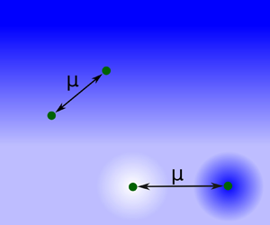
Figure 2. The  $\epsilon ^1 \kappa ^1$ contribution to the far field flow produced by a sphere subject to a force within the viscosity gradient for different directions of the force. The colour indicates the ratio between the $\epsilon ^1 \kappa ^1$ correction flow and the velocity $U^{(0)} = F_1/(6 {\rm \pi}\eta ^{(0)} a)$ at which the particle would move in constant viscosity $\eta ^{(0)}$ when subject to the force $\boldsymbol {F}_1$.
When the force  $\boldsymbol {F}_1$ is applied parallel to the viscosity gradient, it causes an $\epsilon ^1 \kappa ^1$ flow directed inwards along the direction of the viscosity gradient, and a flow directed outwards in the direction orthogonal to the gradient (figure 2a). When the force is acting in the opposite direction, i.e. down the viscosity gradient, also the correction flow field inverts (figure 2b), as a direct consequence of the linearity of the problem. Qualitatively, this effect can be understood as follows: in the region above the particle, the fluid has higher viscosity and hence will react more weakly to the force than a constant-viscosity fluid. Therefore, the correction flow field is oriented oppositely to the force here. In the region below the particle with decreased viscosity, the fluid reacts more strongly and the correction flow is therefore parallel to the force.
When the force is acting perpendicular to the viscosity gradient (figure 2c), the correction flow again follows the direction of the force in the region of lower viscosity, and opposes it in the region of higher viscosity. On the axis perpendicular to the viscosity gradient, a correction flow perpendicular to the force applied is found, such that again a pattern of inwards flow and outwards flow is observed. When the force on the particle at the origin acts in some arbitrary direction (figure 2d), the resulting flow field will be a linear superposition of the flow fields in figures 2(a,c).
As an important consequence of the correction to the mobility matrix (4.5), the far field correction flow at position  $\boldsymbol {r}$ depends only on the direction of $\boldsymbol {r}$ but is constant with respect to the absolute value of the distance, i.e. it does not decay radially. This contrasts with the constant-viscosity Oseen tensor, which decays with the first power of the inverse distance from the particle. However, this correction flow field is valid only as long as the particle separation is, by order of magnitude, smaller than $d$. Therefore, the correction flow, being proportional to $\epsilon \kappa$, always compares small to the Stokeslet flow field, which scales as $a/s$. Consequently, the ratio of the correction to the constant-viscosity term at distances of ${O}(s)$ scales as $\epsilon \kappa /(a/s) = \epsilon s/d$. Inserting values from the experimental system in Stehnach et al. (Reference Stehnach, Waisbord, Walkama and Guasto2021), we obtain $\epsilon \approx 0.5$ for the strongest viscosity gradient considered, which is of total size $2d = 1$ mm. Assuming that the interacting objects (particles or Chlamydomonas cells of size of $\sim 10 \mathrm {\mu }$m) have a distance of $100\ \mathrm {\mu }$m, we find that the first-order correction amounts to the order of 10 % of the constant-viscosity term.
The  $\boldsymbol {\mu }^{(1) rt}_{21}$ term in (4.5) corresponds to the angular velocity $\boldsymbol {\varOmega }^{(1)}_F$ of particle 2 when particle 1 is subject to a force. With $\boldsymbol {r}_1 = \boldsymbol {0}$ and $\boldsymbol {r}_2 = \boldsymbol {r}$, we find
 \begin{equation} \boldsymbol{\varOmega}^{(1)}_F(\boldsymbol{r}) = \boldsymbol{\varOmega}_2^{(1)} = \frac{1}{6 {\rm \pi}a (\eta^{(0)})^2}\,\frac{3a}{8|\boldsymbol{r}|^3}[(\boldsymbol{r} \boldsymbol{\cdot} \boldsymbol{\nabla} \eta^{(1)}) (\boldsymbol{r} \times) + (\boldsymbol{r} \times \boldsymbol{\nabla} \eta^{(1)}) \otimes \boldsymbol{r}] \boldsymbol{\cdot} \boldsymbol{F}_1, \end{equation}
where the first summand results from  $\eta ^{(1)} ((\boldsymbol {r}_1 + \boldsymbol {r}_2)/2) {\boldsymbol{\mathsf{V}}}$ and the second summand results from ${\boldsymbol{\mathsf{Y}}}^\textrm {T}$.
From the  $\boldsymbol {\mu }^{(1) tr}_{21}$ term in the mobility matrix (4.5), we extract the flow field that a particle subject to a torque induces in the viscosity gradient. Assuming that, similarly to before, the viscosity perturbation vanishes at the position of the first particle, the velocity of the second particle acting as a test particle is then given as
 \begin{align} \boldsymbol{u}^{(1)}_T (\boldsymbol{r}) = \boldsymbol{U}_2^{(1)} = \frac{1}{6 {\rm \pi}a (\eta^{(0)})^2}\,\frac{3a}{8|\boldsymbol{r}|^3} [(\boldsymbol{\nabla} \eta^{(1)} \boldsymbol{\cdot} \boldsymbol{r}) (\boldsymbol{r} \times \boldsymbol{T}_1) + \boldsymbol{r} ( (\boldsymbol{r} \times \boldsymbol{\nabla} \eta^{(1)}) \boldsymbol{\cdot} \boldsymbol{T}_1)]. \end{align}
 If a torque acts orthogonal to the viscosity gradient (figure 3a), then a correction flow predominantly in the direction of  $\boldsymbol {\nabla } \eta \times \boldsymbol {T}_1$ is induced. This result holds strictly at $z = 0$, while for $z \neq 0$ an additional component of the flow in the $z$-direction is found. This finding is intuitive since the particle itself moves in the same direction as a result of the correction to its self-mobility. For a torque parallel to the viscosity gradient (figure 3b), an additional rotating flow is observed that has the direction of rotation prescribed by $\boldsymbol {T}_1$ in the region of lower viscosity (here $z < 0$) and opposite direction in the region of increased viscosity (here $z > 0$). In the plane $z = 0$, the correction flow vanishes. Also, this is intuitive, because the fluid opposes the rotation more strongly in the region of higher viscosity, thus resulting in a correction flow with opposite direction of rotation, and the opposite effect in the lower-viscosity region.

Figure 3. Far field  $\epsilon ^1 \kappa ^1$ correction flow induced by a particle subject to an externally applied torque along the direction indicated by the blue arrow, with the direction of the viscosity gradient (a) orthogonal to it, and (b) parallel to it. The colours of the arrows indicate the ratio of the $\epsilon ^1 \kappa ^1$ correction flow and $\varOmega ^{(0)} a$, where $\varOmega ^{(0)} = 1/(8 {\rm \pi}\eta ^{(0)} a^3) |\boldsymbol {T}_1|$ is the angular velocity of the particle in constant viscosity $\eta ^{(0)}$ when subject to the torque $\boldsymbol {T}_1$.
In both cases, the correction flow decays radially as  $r^{-1}$, i.e. by one order slower than in the constant-viscosity case where the rotlet decays as $r^{-2}$. Similarly to the flow field induced by a particle subject to a force, the correction flow field resulting from the linear viscosity gradient decays by one order slower than the constant-viscosity field does, and the ratio of the correction flow to the flow at constant viscosity scales as $\epsilon s/d$. A linear viscosity gradient thus induces long-range interactions between the particles, as long as the particle separation is much shorter than the size of the gradient.
The results presented here for the hydrodynamic interaction of particles in a linear viscosity gradient are also valid for more than two particles (Appendix F) as three-body effects decay quicker than  $1/s$, thus particle interaction is pairwise at the level of approximation chosen here.
4.2. Asymmetric particle placement in the viscosity gradient
In the previous subsection, we assumed that the viscosity perturbation is odd symmetric and both particles are located close to the centre of symmetry or the central plane of the interface-like gradient when compared to the gradient size  $d$. Since in a realistic setting the particle positions in the viscosity gradient are arbitrary, here we consider the interacting particles at varying positions within a finite-size gradient, and calculate the effect of the viscosity gradient compared to the interaction in constant viscosity with the local viscosity as reference. But we require that first, the distance between both particles is still smaller than the gradient size, $s \ll d$, and second, the distance of each particle to the boundary of the linear gradient in any spatial direction is of the same order of magnitude as $d$, i.e. we assume that both particles do not come close to the edge of the linear gradient at length scales of $d$.
$d$.
Considering the scaling properties of the integrand in (3.13), it can be shown that only the term  ${\boldsymbol{\mathsf{Q}}}^{(1) tt}_{bc} = \boldsymbol {\mu }^{(1) tt}_{bc} + {O}(s^{-2})$ is affected at order $\epsilon ^1 \kappa ^1$ if the particles are placed asymmetrically within the gradient (yellow particles in figure 1). The other ${\boldsymbol{\mathsf{Q}}}^{(1)}$ terms involving rotation remain unchanged (see § D.1 of Appendix D for details). Since the integral (3.13) is linear in the viscosity perturbation, the correction is now given by
 \begin{equation} {\boldsymbol{\mathsf{Q}}}^{(1) tt}_{asym} ={-} \frac{2}{(6 {\rm \pi}a \eta^{(0)})^2} \int_V [ \eta^{(1)} (\boldsymbol{r}) - \tilde{\eta}^{(1)} (\boldsymbol{r}) ]\,\frac{27 a^2}{8 |\boldsymbol{r} - \boldsymbol{r}_0|^6}\,(\boldsymbol{r} - \boldsymbol{r}_0) \otimes (\boldsymbol{r} - \boldsymbol{r}_0) \, {\rm d} V. \end{equation}
Here,  $\boldsymbol{r}_0$ is a reference point close to the positions of both particles, i.e. $|\boldsymbol{r}_b - \boldsymbol{r}_0| \ll d$ for b = 1, 2. $\tilde{\eta}^{(1)} = \boldsymbol{H}^{(1)} \boldsymbol{\cdot} (\boldsymbol{r} - \boldsymbol{r}_0)$ denotes the linear viscosity gradient extended to infinity, and $\eta^{(0)} =\eta(\boldsymbol{r}_0)$ is the corresponding reference viscosity, such that the first-order viscosity perturbation vanishes at $\boldsymbol{r}_0$. As a consistency check, it can be verified easily that (4.12) vanishes due to symmetry if $\eta ^{(1)} (\boldsymbol {r})$ is odd symmetric about $\boldsymbol {r}_0$. We point out that this correction applies to both the translational self-mobilities ( $\boldsymbol {\mu }^{(1) tt}_{bb}$) as well as the translational interaction terms in the mobility matrix ( $\boldsymbol {\mu }^{(1) tt}_{bc}$ with $b \neq c$). While here we present the correction for particles placed asymmetrically in the interface-like gradient, a similar correction arises if symmetry is broken by the shape of linear region of the viscosity gradient.
The full first-order mobility matrix in the asymmetric case is then given by
 \begin{equation} \boldsymbol{\mu}^{(1)}_{tot} = \boldsymbol{\mu}^{(1)} + \boldsymbol{\mu}^{(1)}_{asym} = \boldsymbol{\mu}^{(1)} + \begin{pmatrix} {\boldsymbol{\mathsf{Q}}}^{(1) tt}_{asym} & {\boldsymbol{\mathsf{Q}}}^{(1) tt}_{asym} & {\boldsymbol{\mathsf{0}}} & {\boldsymbol{\mathsf{0}}} \\[3pt] {\boldsymbol{\mathsf{Q}}}^{(1) tt}_{asym} & {\boldsymbol{\mathsf{Q}}}^{(1) tt}_{asym} & {\boldsymbol{\mathsf{0}}} & {\boldsymbol{\mathsf{0}}} \\[3pt] {\boldsymbol{\mathsf{0}}} & {\boldsymbol{\mathsf{0}}} & {\boldsymbol{\mathsf{0}}} & {\boldsymbol{\mathsf{0}}} \\[3pt] {\boldsymbol{\mathsf{0}}} & {\boldsymbol{\mathsf{0}}} & {\boldsymbol{\mathsf{0}}} & {\boldsymbol{\mathsf{0}}} \\ \end{pmatrix}, \end{equation}
where  $\boldsymbol {\mu }^{(1)}$ is the result from (4.5). The correction due to asymmetry yields an additional velocity term for both particles 1 and 2, if the sum of the forces on both particles does not vanish:
 \begin{equation} \boldsymbol{U}_1^{asym} = \boldsymbol{U}_2^{asym} = {\boldsymbol{\mathsf{Q}}}^{(1) tt}_{asym} \boldsymbol{\cdot} (\boldsymbol{F}_1 + \boldsymbol{F}_2). \end{equation}
Notably, it is the sum of both forces that induces the additional velocity, such that a force-free particle 1 experiences the same additional velocity from the asymmetry as particle 2, if particle 2 is subject to a force.
To illustrate this effect, we consider the particles to be located near a point with  $y_0 = y'_0 d$ within the interface-like viscosity gradient, where $y'_0$ is independent of $d$, and $\eta ^{(0)}$ is the reference viscosity at $y_0$. The correction term ${\boldsymbol{\mathsf{Q}}}^{(1) tt}_{asym}$ in dependence of $y_0$ is then calculated in § D.5 of Appendix D
 \begin{equation} {\boldsymbol{\mathsf{Q}}}^{(1) tt}_{asym} = \frac{1}{6 {\rm \pi}a (\eta^{(0)})^2}\,\frac{9 a |\boldsymbol{\nabla} \eta^{(1)}|}{16} {\rm arctanh}(y_0/d)\,( {\boldsymbol{\mathsf{I}}} + \boldsymbol{e}_y \otimes \boldsymbol{e}_y).\end{equation}
The dependence of this correction term on the relative position in the viscosity gradient is illustrated in figure 4, with the arrows indicating the direction and the colour indicating the strength of  $\boldsymbol {U}_1^{asym} = \boldsymbol {U}_2^{asym}$.

Figure 4. Additional velocity  $\boldsymbol {U} = \boldsymbol {U}_1^{asym}$ due to asymmetric particle placement in dependence on the position of both particles in the interface-like viscosity gradient. Since the particles have relative distance $s \ll d$, they can be considered as located at the same position at scales of $d$. (a) The correction from asymmetry for a force $\boldsymbol {F} = \boldsymbol {F}_1 + \boldsymbol {F}_2$ applied along the $y$-axis. (b) The correction for a force applied along the $x$-axis. The colour indicates the ratio between the $\epsilon ^1 \kappa ^1$ correction flow and the velocity $U^{(0)} = F/(6 {\rm \pi}\eta ^{(0)} a)$ at which a particle would move in constant viscosity $\eta ^{(0)}$ when subject to the force $\boldsymbol {F}$.
In the half-slab with higher viscosity ( $y_0 > 0$ in figure 4), $\boldsymbol {U}_1^{asym}$ is parallel to the force, while in the other half of the slab it is directed oppositely to the force. Consistently with the results for odd symmetric gradients, $\boldsymbol {U}_1^{asym}$ vanishes in the central plane of the gradient. Intuitively, this result can be understood as follows: particles placed in the half-slab of higher viscosity have smaller distance to the edge of the linear gradient at higher viscosity than to the low-viscosity edge. Then, relative to the particle position, the fraction of the linear gradient with higher viscosity is smaller than the fraction with lower viscosity. In comparison to an odd symmetric gradient, where those two fractions are the same, a correction along the force is expected and observed, since the odd symmetric gradient overestimates the viscosity in parts of the fluid. This is also clear from (4.12): for $y_0 > 0$, the actual viscosity is smaller than that associated with an odd symmetric viscosity profile with respect to the particles’ position, thus the term in square brackets is negative for parts of the fluid and zero otherwise. The remaining integrand is in general positive, thus the overall result of (4.12) is also positive, corresponding qualitatively to a correction along the direction of the applied force. For particles placed in the lower viscosity half-slab, the effect inverses.
For  $|y_0| \lesssim d/2$, we have $\textrm {arctanh}(y_0/d) \approx y_0/d = {O}(1)$, and ${\boldsymbol{\mathsf{Q}}}^{(1) tt}_{asym}$ is of the same order of magnitude as the first-order mobility term associated with hydrodynamic interaction between the particles in (4.5). The correction due to asymmetry therefore alters the $\epsilon ^1 \kappa ^1$ correction flow produced by a particle significantly as soon as the particles are placed away from the plane of symmetry of the interface-like gradient by a non-negligible fraction of $d$. In figure 5, the correction flow field produced by a particle located at $y_0 = 0.5 d$ with respect to the constant-viscosity flow field at the local viscosity as a reference is displayed. Comparison to the correction flow in a symmetric viscosity gradient (figure 2) shows that an asymmetry has a significant impact on the particle interactions, which is of the same order of magnitude as the correction in the symmetric case. As a general rule, we find that the effect from asymmetry leads to a stronger correction flow field towards the central plane of the gradient, and to a weaker correction field towards the edge of the gradient.

Figure 5. The  $\epsilon ^1 \kappa ^1$ correction far field flow produced by a spherical particle subject to a force and placed asymmetrically in the interface-like viscosity gradient at $y_0 = 0.5 d$, where the local viscosity at the particle is taken as reference. In (a), the force acts along the $y$-direction; in (b), it acts along the $x$-direction. The colour indicates the ratio between the $\epsilon ^1 \kappa ^1$ correction flow and the velocity $U^{(0)} = F_1/(6 {\rm \pi}\eta ^{(0)} a)$ at which the particle would move in constant viscosity $\eta ^{(0)}$ when subject to the force $\boldsymbol {F}_1$.
Interestingly, the leading-order correction to the mobility matrix is affected even if the symmetry of the viscosity gradient is broken at distances of  ${O}(d)$ from the particles, while the viscosity profile at distances of ${O}(s)$ is linear and thus odd symmetric near the particles. This results ultimately from the scaling properties of (4.12) with respect to the gradient size $d$: rescaling the coordinate system by $d$, the viscosity profile in terms of the rescaled position is independent of $d$, while the remaining integrand factors out $1/d^4$ and the volume element scales as $d^3$. Consequently, the overall integral scales as $1/d \sim \boldsymbol {\nabla } \eta ^{(1)}$ (see § D.1 of Appendix D for details). As a result, the hydrodynamics in linear viscosity gradients includes highly non-local effects proportional to the magnitude of the viscosity gradient.
5. Interaction of hot particles
As a second application of the presented method, we calculate the interaction of spherical particles with a homogeneous surface temperature that is different from the temperature of the surrounding fluid. In contrast to the previous case of a linear viscosity gradient assumed to be unperturbed by the presence of particles, the viscosity profile here emerges as direct consequence of the particles’ presence. Hence we first calculate the viscosity profile, and obtain from this the correction to the mobility matrix in a second step.
The dependence of fluid viscosity on temperature can often be approximated using Andrade's equation,  $\eta = A \exp (b/T)$ (Andrade Reference Andrade1930), where $A$ and $b$ are fluid-specific parameters. However, for small temperature contrasts, Taylor expanding Andrade's equation or one of its generalisations (Gutmann & Simmons Reference Gutmann and Simmons1952) yields a linear relation between temperature and fluid viscosity, which we will use in the following. As a result, a single hot particle induces a viscosity perturbation decaying with inverse distance from the particle centre (figure 6), which in turn alters the self-mobility of the particle as shown in Oppenheimer et al. (Reference Oppenheimer, Navardi and Stone2016). However, to the best of our knowledge, no results are available for the interaction of two hot particles, which we determine in the following.

Figure 6. Exemplary sketch of the viscosity perturbation in the presence of a hot particle and a cold particle. The fluid viscosity is smaller in the neighbourhood of the hot particle, and higher in the neighbourhood of the cold particle.
For a two-particle system with prescribed homogeneous surface temperatures, we first assume that a steady state is established by thermal conduction. Consequently, our model requires that the steady state establishes on faster time scales than the particle temperature changes. In practice, this is the case for beads with large heat capacities. The same would occur for objects subject to constant heat radiation if the susceptibility of the particles is different from that of the surrounding fluid. Second, our approach requires a small Péclet number ( $Pe$), which compares advective to thermal heat transport:
 \begin{equation} Pe = \frac{U a}{\kappa} = Re \, Pr, \end{equation}
where  $U$ is the typical velocity in the fluid and $\kappa$ is the thermal diffusivity; $Re$ and $Pr$ denote the Reynolds and Prandtl numbers, and the latter depends only on properties of the fluid (Leal Reference Leal2007, p. 596).
The conduction-induced temperature field around a particle with homogeneous surface temperature in a quiescent fluid, which decays as  $r^{-1}$, typically breaks down at a length scale of ${O}(a / Pe)$ (Leal Reference Leal2007, p. 604). For the subsequent calculation, we assume that $s \ll a/ Pe$, i.e. the distance between the two interacting particles is smaller than the length scale at which the temperature profile in the fluid becomes advection-dominated. Similarly to the single particle mobilities (Oppenheimer et al. Reference Oppenheimer, Navardi and Stone2016), the corresponding correction due to finite $Pe$ then scales asymptotically as ${O}(Pe^2)$ and can be neglected in the limit of small Péclet numbers. Indeed, for a micron-sized particle, for example, moving at a speed of microns per second in water at room temperature, the Reynolds number is ${O}(10^{-6})$, and with $Pr \sim {O}(10)$ (Dincer & Zamfirescu Reference Dincer and Zamfirescu2015, Appendix B), the Péclet number is ${O}(10^{-5})$, such that the above assumptions are indeed valid e.g. for colloidal particles (Lu & Weitz Reference Lu and Weitz2013) separated by up to tens of radii.
Under these assumptions, the temperature field in the fluid is described by the heat equation with prescribed homogeneous temperatures at the particle surfaces ( $T_1$ and $T_2$ respectively) and at infinity ( $T_0$) as boundary conditions:
 \begin{equation} \nabla^2 T(\boldsymbol{r}) = 0, \quad T(\boldsymbol{r}) = T_b\ \mathrm{for} \ \boldsymbol{r} \in S_b, \quad T(\boldsymbol{r}) \to T_0\ \mathrm{for} \ |\boldsymbol{r}| \to \infty, \end{equation}
where  $S_b$ is the surface of particle $b$. For a system consisting of two or more particles, the temperature field can be approximated by a reflection scheme, where monopolar, dipolar, etc. single-particle fields are superposed to match the boundary conditions up to successively increasing order in the inverse particle separation, similarly to the fluid velocity field. We obtain for the temperature field including all terms up to ${O}(s^{-2})$,
 \begin{align} T(\boldsymbol{r}) = T_0 + C^m_1\,\frac{a}{|\boldsymbol{r} - \boldsymbol{r}_1|} + \frac{a^2 \boldsymbol{C}^d_1 \boldsymbol{\cdot} (\boldsymbol{r} - \boldsymbol{r}_1)}{|\boldsymbol{r} - \boldsymbol{r}_1|^3} + C^m_2\,\frac{a}{|\boldsymbol{r} - \boldsymbol{r}_2|} + \frac{a^2 \boldsymbol{C}^d_2 \boldsymbol{\cdot} (\boldsymbol{r} - \boldsymbol{r}_2)}{|\boldsymbol{r} - \boldsymbol{r}_2|^3} + {O}(s^{{-}3}), \end{align}
with
 $$\begin{gather} C^m_1 = {\rm \Delta} T_1 \left(1 + \frac{a^2}{s^2} \right) - {\rm \Delta} T_2\, \frac{a}{s}, \quad \boldsymbol{C}^d_1 ={-} {\rm \Delta} T_2\, \frac{a^2 \boldsymbol{s}}{s^3}, \end{gather}$$
 $$\begin{gather}C^m_2 = {\rm \Delta} T_2 \left( 1 + \frac{a^2}{s^2} \right) - {\rm \Delta} T_1\,\frac{a}{s}, \quad \boldsymbol{C}^d_2 = {\rm \Delta} T_1\,\frac{a^2 \boldsymbol{s}}{s^3}. \end{gather}$$
Approximating the dependence of the viscosity on the temperature as linear, we find
 \begin{equation} \eta \approx \eta^{(0)} + \left. \frac{\partial \eta}{\partial T} \right|_{T_0} (T - T_0)=: \eta^{(0)} + \alpha (T - T_0), \end{equation}
where  $\alpha$ is the proportionality coefficient. For particles with a temperature contrast relative to the fluid, it is natural to assume that $\eta ^{(0)}$ is the viscosity at temperature $T_0$. Assuming that ${\rm \Delta} T_1$ and ${\rm \Delta} T_2$ are typically of the order of some ${\rm \Delta} T$, we define the perturbation parameter $\epsilon := - \alpha \,{\rm \Delta} T/\eta ^{(0)}$ as the relative change in viscosity associated with ${\rm \Delta} T$ compared to $\eta ^{(0)}$ (Oppenheimer et al. Reference Oppenheimer, Navardi and Stone2016). Typically, $\alpha$ is negative, associating hot particles ( $T > T_0$) with a decrease in viscosity, and cold particles ( $T < T_0$) with an increase, thus $\epsilon$ is positive (Gutmann & Simmons Reference Gutmann and Simmons1952).
Using (5.6) and the definition of  $\epsilon$, the $\epsilon ^1$ viscosity perturbation is given as
 \begin{equation} \eta^{(1)} = -\eta^{(0)}\,\frac{T(\boldsymbol{r}) - T_0}{{\rm \Delta} T}. \end{equation}
By inserting the expression for the temperature field (5.3), we obtain the explicit expansion of the viscosity field:
 \begin{align}
\eta^{(1)}(\boldsymbol{r}) &= \eta^{(1)
m}_1\,\frac{a}{|\boldsymbol{r} - \boldsymbol{r}_1|} +
\frac{a^2 \boldsymbol{\eta}^{(1) d}_1 \boldsymbol{\cdot}
(\boldsymbol{r} - \boldsymbol{r}_1)}{|\boldsymbol{r} -
\boldsymbol{r}_1|^3} + \eta^{(1)
m}_2\,\frac{a}{|\boldsymbol{r} - \boldsymbol{r}_2|}\nonumber\\ &\quad +
\frac{a^2 \boldsymbol{\eta}^{(1) d}_2 \boldsymbol{\cdot}
(\boldsymbol{r} - \boldsymbol{r}_2)}{|\boldsymbol{r} -
\boldsymbol{r}_2|^3} + {O}(s^{{-}3}),
\end{align}
\begin{align}
\eta^{(1)}(\boldsymbol{r}) &= \eta^{(1)
m}_1\,\frac{a}{|\boldsymbol{r} - \boldsymbol{r}_1|} +
\frac{a^2 \boldsymbol{\eta}^{(1) d}_1 \boldsymbol{\cdot}
(\boldsymbol{r} - \boldsymbol{r}_1)}{|\boldsymbol{r} -
\boldsymbol{r}_1|^3} + \eta^{(1)
m}_2\,\frac{a}{|\boldsymbol{r} - \boldsymbol{r}_2|}\nonumber\\ &\quad +
\frac{a^2 \boldsymbol{\eta}^{(1) d}_2 \boldsymbol{\cdot}
(\boldsymbol{r} - \boldsymbol{r}_2)}{|\boldsymbol{r} -
\boldsymbol{r}_2|^3} + {O}(s^{{-}3}),
\end{align}
with  $\eta ^{(1) m}_b = -(\eta ^{(0)} C^m_b)/{\rm \Delta} T$ and $\boldsymbol {\eta }^{(1) d}_b = -(\eta ^{(0)} \boldsymbol {C}^d_b)/{\rm \Delta} T$, $b \in \{1, 2\}$.
Using (5.8), we first calculate the respective  ${\boldsymbol{\mathsf{Q}}}^{(1)}$ terms (Appendix E) and from this compute the $\epsilon ^1$ correction to the mobility matrix. One can show that, up to ${O}(s^{-2})$, the corrections to the mobility matrix are given by the corresponding ${\boldsymbol{\mathsf{Q}}}^{(1)}$ terms (§ E.3 of Appendix E):
 \begin{equation} \boldsymbol{\mu}^{(1)PQ}_{bc} = {\boldsymbol{\mathsf{Q}}}^{(1)PQ}_{bc} + {O}(s^{{-}3}). \end{equation}
We then find the  $\epsilon ^1$ correction to the mobility matrix given by
 \begin{align} \left. \begin{array}{c@{}}
\boldsymbol{\mu}^{(1)tt}_{bb} = \dfrac{1}{6 {\rm \pi}a
\eta^{(0)}} \left[ \left( \left(\dfrac{5}{12} - \dfrac{7
a^2}{12 s^2} \right) \dfrac{{\rm \Delta} T_b}{{\rm \Delta} T} +
\left( \dfrac{7 a}{12 s} - \dfrac{9 a^2}{8 s^2} \right)
\dfrac{{\rm \Delta} T_c}{{\rm \Delta} T} \right)
{\boldsymbol{\mathsf{I}}} + \dfrac{9 a^2}{8}\,
\dfrac{{\rm \Delta} T_c}{{\rm \Delta} T}\,\dfrac{\boldsymbol{s}
\otimes \boldsymbol{s}}{s^4} \right]\\ \hspace{-21pc}+\, {O}(s^{{-}3}), \\ \boldsymbol{\mu}^{(1)rr}_{bb} = \dfrac{1}{6 {\rm \pi}a
\eta^{(0)}} \left[ \left(\dfrac{9}{16 a^2} - \dfrac{3}{16
s^2} \right) \dfrac{{\rm \Delta} T_b}{{\rm \Delta} T} + \dfrac{3}{16
as}\,\dfrac{{\rm \Delta} T_c}{{\rm \Delta} T} \right]
{\boldsymbol{\mathsf{I}}} + {O}(s^{{-}3}), \\
\boldsymbol{\mu}^{(1) tr}_{11} = \dfrac{1}{6 {\rm \pi}a
\eta^{(0)}} \left( -\dfrac{{\rm \Delta} T_2}{{\rm \Delta}
T}\,\dfrac{a (\boldsymbol{s} \times)}{8 s^3} \right) +
{O}(s^{{-}3}) ={-}\boldsymbol{\mu}^{(1) rt}_{11},\\
\boldsymbol{\mu}^{(1) tr}_{22} = \dfrac{1}{6 {\rm \pi}a
\eta^{(0)}} \left( \dfrac{{\rm \Delta} T_1}{{\rm \Delta} T}\,
\dfrac{a (\boldsymbol{s} \times)}{8 s^3} \right) +
{O}(s^{{-}3}) ={-}\boldsymbol{\mu}^{(1) rt}_{22},\\
\boldsymbol{\mu}^{(1)tt}_{bc} = \dfrac{1}{6 {\rm \pi}a
\eta^{(0)}} \left( \dfrac{9 a^2}{8}\,\dfrac{{\rm \Delta} T_b +
{\rm \Delta} T_c}{{\rm \Delta} T}\,\dfrac{\boldsymbol{s} \otimes
\boldsymbol{s}}{s^4} \right) + {O}(s^{{-}3}), \quad b \neq
c, \\ \boldsymbol{\mu}^{(1)tr}_{bc} =
\boldsymbol{\mu}^{(1) rt}_{bc} = \boldsymbol{\mu}^{(1)
rr}_{bc} = {O}(s^{{-}3}), \quad b \neq c .
\end{array}\right\} \end{align}
\begin{align} \left. \begin{array}{c@{}}
\boldsymbol{\mu}^{(1)tt}_{bb} = \dfrac{1}{6 {\rm \pi}a
\eta^{(0)}} \left[ \left( \left(\dfrac{5}{12} - \dfrac{7
a^2}{12 s^2} \right) \dfrac{{\rm \Delta} T_b}{{\rm \Delta} T} +
\left( \dfrac{7 a}{12 s} - \dfrac{9 a^2}{8 s^2} \right)
\dfrac{{\rm \Delta} T_c}{{\rm \Delta} T} \right)
{\boldsymbol{\mathsf{I}}} + \dfrac{9 a^2}{8}\,
\dfrac{{\rm \Delta} T_c}{{\rm \Delta} T}\,\dfrac{\boldsymbol{s}
\otimes \boldsymbol{s}}{s^4} \right]\\ \hspace{-21pc}+\, {O}(s^{{-}3}), \\ \boldsymbol{\mu}^{(1)rr}_{bb} = \dfrac{1}{6 {\rm \pi}a
\eta^{(0)}} \left[ \left(\dfrac{9}{16 a^2} - \dfrac{3}{16
s^2} \right) \dfrac{{\rm \Delta} T_b}{{\rm \Delta} T} + \dfrac{3}{16
as}\,\dfrac{{\rm \Delta} T_c}{{\rm \Delta} T} \right]
{\boldsymbol{\mathsf{I}}} + {O}(s^{{-}3}), \\
\boldsymbol{\mu}^{(1) tr}_{11} = \dfrac{1}{6 {\rm \pi}a
\eta^{(0)}} \left( -\dfrac{{\rm \Delta} T_2}{{\rm \Delta}
T}\,\dfrac{a (\boldsymbol{s} \times)}{8 s^3} \right) +
{O}(s^{{-}3}) ={-}\boldsymbol{\mu}^{(1) rt}_{11},\\
\boldsymbol{\mu}^{(1) tr}_{22} = \dfrac{1}{6 {\rm \pi}a
\eta^{(0)}} \left( \dfrac{{\rm \Delta} T_1}{{\rm \Delta} T}\,
\dfrac{a (\boldsymbol{s} \times)}{8 s^3} \right) +
{O}(s^{{-}3}) ={-}\boldsymbol{\mu}^{(1) rt}_{22},\\
\boldsymbol{\mu}^{(1)tt}_{bc} = \dfrac{1}{6 {\rm \pi}a
\eta^{(0)}} \left( \dfrac{9 a^2}{8}\,\dfrac{{\rm \Delta} T_b +
{\rm \Delta} T_c}{{\rm \Delta} T}\,\dfrac{\boldsymbol{s} \otimes
\boldsymbol{s}}{s^4} \right) + {O}(s^{{-}3}), \quad b \neq
c, \\ \boldsymbol{\mu}^{(1)tr}_{bc} =
\boldsymbol{\mu}^{(1) rt}_{bc} = \boldsymbol{\mu}^{(1)
rr}_{bc} = {O}(s^{{-}3}), \quad b \neq c .
\end{array}\right\} \end{align}
The corrections to the translational and rotational self-mobilities of, say, particle 1 depend at order  $s^0$ only on the particle's own temperature, which alters the self-mobility similarly as in the case when there is only one particle in the fluid (Oppenheimer et al. Reference Oppenheimer, Navardi and Stone2016). If the particle is hot, i.e. $T_1 > T_0$, then the particle's mobility increases, and it decreases for $T_1 < T_0$.
In contrast to the case of a single particle, we find additional terms scaling as  $s^{-1}$ in the first particle's translational and rotational self-mobilities, which are proportional to the temperature of the second particle at the distance $s$. This is because the temperature of particle 2 induces a radially decaying temperature and viscosity field around it, which can be approximated to leading order as constant near particle 1. In order to satisfy the boundary condition for the temperature field at the surface of particle 1, a reflected monopolar temperature field around particle 1 is induced. However, the reflected flow field decays as $r^{-1}$, where $r$ is the distance from particle 1. Therefore, the effect due to the incident field is stronger than the effect of the reflected field, and the mobility of particle 1 indeed increases for a hot particle 2, and decreases if particle 2 has a lower temperature than the fluid at infinity. Consequently, the ratio of magnitudes of the correction to self-mobility due to the presence of the second particle and the single-particle self-mobility of a neutral particle scales as $\epsilon a/s$.
While for a single particle with homogeneous surface temperature translation and rotation do not couple (Oppenheimer et al. Reference Oppenheimer, Navardi and Stone2016), such coupling is observed at  ${O}(s^{-2})$ in the presence of a second particle. This effect on, say, particle 1 can be understood as the result of the gradient of the monopolar temperature field induced by particle 2. However, also here a dipolar temperature field reflected from particle 1 arises to satisfy the boundary conditions at the surface of particle 1, and weakens the effect of the incident temperature gradient.
Considering the components associated with hydrodynamic interactions between particles in (5.10), only the translational term is non-vanishing at our level of approximation, and it scales as  $1/s^2$. Interestingly, the translational interaction between two particles increases proportional to the sum ${\rm \Delta} T_1 + {\rm \Delta} T_2$, i.e. it is irrelevant whether the particle causing or experiencing the interaction has an altered temperature. This observation is in agreement with the fact that the mobility matrix is symmetric as a result of the Lorentz reciprocal theorem (Jeffrey & Onishi Reference Jeffrey and Onishi1984), a result that holds independently of whether or not the viscosity is constant. Moreover, if one particle is hotter and the other is colder than the fluid by the same amount, then the effects cancel and the interaction between the particles is, up to order ${O}(s^{-2})$, similar to the interaction of two neutral particles.
Considering the second particle as a neutral test particle, i.e.  ${\rm \Delta} T_2 = 0$, for the far field correction flow produced by particle 1 located at $\boldsymbol {r} = \boldsymbol {0}$ with increased temperature ${\rm \Delta} T_1 > 0$ and subject to a force $\boldsymbol {F}_1$, we find
 \begin{equation} \boldsymbol{u}^{(1)} (\boldsymbol{r}) = \boldsymbol{U}_2^{(1)} = \frac{1}{6 {\rm \pi}a \eta^{(0)}}\, \frac{9 a^2 {\rm \Delta} T_1}{8 r^4 {\rm \Delta} T}\,\boldsymbol{r} (\boldsymbol{r} \boldsymbol{\cdot} \boldsymbol{F}_1). \end{equation}
This flow field decays with the second power of the distance from particle 1 and is depicted in figure 7. Along the direction of the force applied, the correction flow is parallel to the force, thus enhancing the constant viscosity Stokeslet flow. This is reasonable since with increased temperature, the viscosity around the particle is decreased and the flow field becomes stronger. However, on the axis perpendicular to the force, the correction flow vanishes, concentrating the correction flow along the direction of the force applied. As a consistency check, we find that the divergence of the flow field (5.11) vanishes, thus the flow satisfies the incompressibility condition. In contrast to a linear viscosity gradient, this correction flow field decays more strongly than the constant-viscosity Stokeslet by one order. The ratio of the first-order correction in the mobility term for particle interaction and the constant-viscosity term thus also scales as  $\epsilon a/s$, and hence can be important in application.

Figure 7. The  $\epsilon ^1$ far field correction flow field produced by a hot particle with a force applied along the $x$-direction. The colour indicates the ratio of the first-order correction flow and the velocity $U^{(0)} = F_1/( 6 {\rm \pi}\eta ^{(0)} a)$, at which the particle would move if it had the same temperature as the surrounding fluid, $T_1 = T_0$, and was subject to the force $\boldsymbol {F}_1$.
In comparison to the case of linear viscosity gradients (§ 4), three-body effects affect the correction to the mobility matrix already at the level of approximation considered, namely at  ${O}(s^{-2})$. For instance, a third particle 3 will in general induce a reflected temperature and viscosity field in response to the temperature of particle 2. At the position of particle 1, this reflected field then scales as $1/s^2$, assuming that all inter-particle distances are of ${O}(s)$. Consequently, the self-mobility of particle 1 will be altered at ${O}(s^{-2})$ by a proper three-body effect. Even more importantly, the correction to the mobility term associated with interaction between two particles 1 and 2 will also be altered at ${O}(s^{-2})$ by the temperature of a nearby particle 3. This is because particle 3 heats or cools the fluid in between particles 1 and 2 in a similar way as particles 1 and 2 do.
6. Conclusion
In this work, we have presented a framework to calculate the first-order correction to the mobility matrix of spherical particles in viscosity gradients, and have illustrated this result for a large linear viscosity gradient and for the viscosity perturbations due to the particle temperature in the limit of low Péclet number.
For a linear viscosity gradient, we have shown that the leading-order correction to the interaction is independent of the distance between the particles, a result that is valid as long as the particle separation is small compared to the size of the viscosity gradient. The result found is in agreement with the generalised Oseen tensor derived in Laumann & Zimmermann (Reference Laumann and Zimmermann2019). The increase in the exponent associated with the radial decay results ultimately from the viscosity being a linear field and therefore lifting the exponent by 1 in the corresponding integrals. Similarly, the flow field produced by a particle subject to a torque, which scales with the second inverse power of the distance to the particle in constant viscosity, experiences a correction due to the viscosity gradient that decays slower by one order. In contrast to the case of constant viscosity, a viscosity gradient induces hydrodynamic particle interactions with a component orthogonal to the connection line even if the force is applied along the separation. The ratio of the first-order correction to the interaction terms in the mobility matrix and the corresponding constant-viscosity terms scales as  $\epsilon s/d$ for both translation and rotation. In experimental systems (Stehnach et al. Reference Stehnach, Waisbord, Walkama and Guasto2021), where the assumptions $d \gg s \gg a$ are satisfied, the first-order correction thus can amount to the order of 10 % of the constant viscosity term, thus the corrections presented will be important. The results for the mobility matrix presented here are valid not only for two-particle systems but extend, at the level of approximation chosen, to many particles since three-body and higher-order effects decay quicker than $1/s$. Therefore, the results presented here are also applicable to dilute suspensions of many interacting particles.
In addition, we have shown that if both particles are placed away from the centre of symmetry of the gradient, or if the gradient is not odd symmetric, then translational self-mobilities and interactions have to be corrected with respect to the symmetric case by an additional term. This feature is important since in experimental systems, viscosity gradients are of finite size and the particle position can be arbitrary. This correction has, to the best of our knowledge, not been reported yet. It alters, in particular, the far field flow produced by a particle subject to an external force (figure 5) and becomes relevant already when the particles are placed away from the centre of symmetry by only a fraction of the gradient size. For asymmetric particle placement in an interface-like viscosity gradient, the resulting flow field is typically stronger towards the centre of symmetry and is weaker towards the edge of the viscosity gradient.
For particles at temperatures different to that of the surrounding fluid, we calculated the resulting temperature and viscosity fields in the fluid using a reflection method. We assumed that the Péclet number is small such that at length scales of the particle separation, conductive effects dominate over advective effects. In this case, the self-mobilities of both particles are increased for hot and decreased for cold particles already at the zeroth order in  $s$. At this order, our results are in exact agreement with the findings presented in Oppenheimer et al. (Reference Oppenheimer, Navardi and Stone2016). In addition, however, we found that at the next higher order in the inverse particle separation, the self-mobilities become higher or lower by the presence of a nearby particle with increased or decreased temperature relative to the surrounding fluid, respectively. Essentially, the second particle heats up or cools down the environment of the first particle, and alters its mobility. The ratio of this effect and the constant-viscosity self-mobility scales as $\epsilon a/s$, and thus becomes important for strong temperature differences between particle and fluid. Finally, while for a single particle with a homogeneous surface temperature no coupling between translation and rotation is observed (Oppenheimer et al. Reference Oppenheimer, Navardi and Stone2016), such a term arises due to the presence of a second hot or cold particle, and scales with the second inverse power of the particle separation.
The correction to the hydrodynamic interaction between two different hot or cold particles scales to leading order with the second inverse power of the particle separation and is proportional to the sum of the temperature differences of both particles with respect to the fluid. Thus whether the particle producing the flow or the particle sensing the flow has an increased or decreased temperature has no effect on the interaction between the two. This is a consequence of the symmetry of the mobility matrix. In comparison to the constant-viscosity Stokeslet, this correction term decays quicker by one order in the particle separation, which coincides with the fact that the viscosity perturbation scales to leading order as  $s^{-1}$. Consequently, the ratio of the first-order correction to the mobility term associated with hydrodynamic interaction and the respective constant-viscosity term also scales as $\epsilon a/s$.
In typical situations where the viscosity perturbation results from the dependence of the viscosity on another quantity, such as e.g. temperature or solvent concentration, the presence of the particles can affect an ambient viscosity gradient in dependence of the boundary conditions imposed at the particle surface. In particular, it has been demonstrated recently that the presence of a particle locally disturbs a linear viscosity gradient in dependence of the particle's heat conductivity and the boundary condition applied (Shaik & Elfring Reference Shaik and Elfring2021). The framework presented here can be applied to such more complex situations by combining the tools presented for the specific cases of externally prescribed linear gradients and hot particles. Namely, after calculating the viscosity profile in the fluid emerging from e.g. the fluid temperature field, including the disturbances by the particles, the calculation of the correction to the mobility matrix by the formulas presented will involve both linear and radial viscosity fields. While the variety of such systems is beyond the scope of this paper, we believe that the methodology presented will prove useful for other researchers as it can be applied to the specific system of interest.
The results presented here may shed new light on many particulate systems featuring non-constant viscosity. A notable example is the behaviour of microswimmers, which are often modelled as machines composed of spherical particles (Najafi & Golestanian Reference Najafi and Golestanian2004; Friedrich & Jülicher Reference Friedrich and Jülicher2012; Reigh, Winkler & Gompper Reference Reigh, Winkler and Gompper2012; Elgeti & Gompper Reference Elgeti and Gompper2013), in such an environment reigned by viscosity gradients. A main finding in Liebchen et al. (Reference Liebchen, Monderkamp, Ten Hagen and Löwen2018) was that uniaxial swimmers, i.e. particle-based swimmers with all beads on a common axis, do not adjust their swimming direction due to a viscosity gradient when the  $\epsilon ^1$ correction to the particle interaction is neglected. Essentially, this is because all forces act along the common axis such that this axis must be preserved in time. However, our results show that in such an arrangement of the particles, the first-order correction to the hydrodynamic particle interaction can induce particle motion orthogonal to the common axis when the axis itself is not aligned with the gradient (figure 2c). Hence the correction terms to particle interaction found here might allow for a rotation due to the viscosity gradient also for uniaxial swimmers (Najafi & Golestanian Reference Najafi and Golestanian2004; Dombrowski & Klotsa Reference Dombrowski and Klotsa2020; Hubert et al. Reference Hubert, Trosman, Collard, Sukhov, Harting, Vandewalle and Smith2021). Such a result would coincide with the recently reported viscotaxis for uniaxial squirmers (Datt & Elfring Reference Datt and Elfring2019; Shaik & Elfring Reference Shaik and Elfring2021).
Also, the viscotactic behaviour of Chlamydomonas has recently been characterised experimentally (Stehnach et al. Reference Stehnach, Waisbord, Walkama and Guasto2021). Since modelling Chlamydomonas cells using a triangular swimmer consisting of three beads (Rizvi, Farutin & Misbah Reference Rizvi, Farutin and Misbah2018; Ziegler et al. Reference Ziegler, Hubert, Vandewalle, Harting and Smith2019) has already been established in the literature (Friedrich & Jülicher Reference Friedrich and Jülicher2012; Bennett & Golestanian Reference Bennett and Golestanian2013), our results can be applied directly for a better understanding of their behaviour in a viscosity gradient. Moreover, a more precise result for the correction to the mobility matrix in terms of the inverse particle separation can also be used to understand cilia and flagella within viscosity gradients, which also can be approximated by a set of spherical particles (Reigh et al. Reference Reigh, Winkler and Gompper2012; Elgeti & Gompper Reference Elgeti and Gompper2013). We plan to address the impact of our results on the viscotaxis of microswimmers in a future publication.
The results and methods presented here might also shed new light on the collective behaviour of Janus particles driven by laser light (Buttinoni et al. Reference Buttinoni, Volpe, Kümmel, Volpe and Bechinger2012; Bäuerle et al. Reference Bäuerle, Fischer, Speck and Bechinger2018), where the incident radiation leads to an increase in particle temperature and thus also to viscosity gradients around the particles. Besides the context of microswimmers, the results presented could also prove useful in sedimentation and centrifugation of nanoparticles, which often feature density and viscosity gradients (Qiu & Mao Reference Qiu and Mao2011; Plüisch et al. Reference Plüisch, Bössenecker, Dobler and Wittemann2019), or in diffusion of particles or polymers through a pore featuring a viscosity gradient (De Haan & Slater Reference De Haan and Slater2013). This holds in particular for systems with higher particle concentration, where interaction effects become relevant. Furthermore, viscosity gradients are abundant in biological environments with low Reynolds number (Swidsinski et al. Reference Swidsinski, Sydora, Doerffel, Loening-Baucke, Vaneechoutte, Lupicki, Scholze, Lochs and Dieleman2007; Wilking et al. Reference Wilking, Angelini, Seminara, Brenner and Weitz2011), and the results presented here may lead to a better understanding of the interaction of active components therein.
Acknowledgements
The authors thank M. Hubert and A. Baer for valuable discussions.
Funding
The authors acknowledge support by the German Research Foundation (DFG) within the Collaborative Research Center 1411 ‘Design of Particulate Products’.
Declaration of interests
The authors report no conflict of interest.
Data availability statement
Data sharing is not applicable to this article as no new data were created or analysed in this study.
Appendix A. Derivation of the Lorentz reciprocal theorem
Finding the mobility and resistance matrix of an ensemble of particles in the general case of non-constant viscosity corresponds to solving the boundary-value problem given by the Stokes equations (2.2a,b) for the fluid velocity with the boundary conditions (Oppenheimer et al. Reference Oppenheimer, Navardi and Stone2016)
 \begin{equation} \boldsymbol{u} (\boldsymbol{r}) = \boldsymbol{U}_b + \boldsymbol{\varOmega}_b \times (\boldsymbol{r} - \boldsymbol{r}_b) \forall \, \boldsymbol{r} \in S_b, \quad \boldsymbol{u}(\boldsymbol{r}) \to 0,\ p(\boldsymbol{r}) \to 0\ \mathrm{for} \ \boldsymbol{r} \to \infty, \end{equation}
at the surfaces of the particles  $S_b$ and at infinity, respectively. With prescribed (angular) particle velocities $\boldsymbol {U}_b$ and $\boldsymbol {\varOmega }_b$, the hydrodynamic forces and torques acting on the particles are obtained by Oppenheimer et al. (Reference Oppenheimer, Navardi and Stone2016) as
 \begin{equation} \boldsymbol{F}^{hydro}_b = \int_{S_b} \boldsymbol{n} \boldsymbol{\cdot} \boldsymbol{\sigma}\, {\rm d} S, \quad \boldsymbol{T}^{hydro}_b = \int_{S_b} (\boldsymbol{r} - \boldsymbol{r}_b) \times (\boldsymbol{n} \boldsymbol{\cdot} \boldsymbol{\sigma})\, {\rm d} S. \end{equation}
They then yield the resistance matrix by means of (2.5). Here,  $\textrm {d} S$ denotes the infinitesimal area element, and $\boldsymbol {n}$ the normal vector directed into the fluid. With these expressions at hand, we exploit the Lorentz reciprocal theorem to derive the first-order correction in $\epsilon$ to the mobility matrix.
Following Oppenheimer et al. (Reference Oppenheimer, Navardi and Stone2016), we calculate
 \begin{align} 0 &= (\boldsymbol{\nabla} \boldsymbol{\cdot} \boldsymbol{\sigma}) \boldsymbol{\cdot} \boldsymbol{u}^{(0)} = \boldsymbol{\nabla} \boldsymbol{\cdot} (\boldsymbol{\sigma} \boldsymbol{\cdot} \boldsymbol{u}^{(0)}) - \boldsymbol{\sigma} : \boldsymbol{\nabla} \boldsymbol{u}^{(0)} \nonumber\\ &= \boldsymbol{\nabla} \boldsymbol{\cdot} (\boldsymbol{\sigma} \boldsymbol{\cdot} \boldsymbol{u}^{(0)}) - ({-}p {\boldsymbol{\mathsf{I}}} + 2 \eta(\boldsymbol{r})\,{\boldsymbol{\mathsf{E}}} ) : \boldsymbol{\nabla} \boldsymbol{u}^{(0)} = \boldsymbol{\nabla} \boldsymbol{\cdot} (\boldsymbol{\sigma} \boldsymbol{\cdot} \boldsymbol{u}^{(0)}) - 2 \eta(\boldsymbol{r})\,{\boldsymbol{\mathsf{E}}} : {\boldsymbol{\mathsf{E}}}^{(0)}, \end{align}
where in the last step we have used that  ${\boldsymbol{\mathsf{I}}} : \boldsymbol {\nabla } \boldsymbol {u}^{(0)} = 0$ due to incompressibility, and ${{\boldsymbol{\mathsf{E}}} : \boldsymbol {\nabla } \boldsymbol {u}^{(0)} = {\boldsymbol{\mathsf{E}}} : {\boldsymbol{\mathsf{E}}}^{(0)}}$ because ${\boldsymbol{\mathsf{E}}}$ is a symmetric tensor. By ’ $:$’ we denote the contraction of the last two indices of the first tensor with the first two indices of the second tensor, i.e. ${\boldsymbol{\mathsf{E}}} : {\boldsymbol{\mathsf{E}}}^{(0)} :=\textsf {{E}}_{kl} \textsf {{E}}^{(0)}_{kl}$.
With the same argument we find that
 \begin{equation} 0 = (\boldsymbol{\nabla} \boldsymbol{\cdot} \boldsymbol{\sigma}^{(0)}) \boldsymbol{\cdot} \boldsymbol{u} = \boldsymbol{\nabla} \boldsymbol{\cdot} (\boldsymbol{\sigma}^{(0)} \boldsymbol{\cdot} \boldsymbol{u}) - 2 \eta^{(0)} {\boldsymbol{\mathsf{E}}} : {\boldsymbol{\mathsf{E}}}^{(0)}. \end{equation}
By taking the difference of (A3) and (A4), we obtain
 \begin{equation} \boldsymbol{\nabla} \boldsymbol{\cdot} (\boldsymbol{\sigma} \boldsymbol{\cdot} \boldsymbol{u}^{(0)}) - \boldsymbol{\nabla} \boldsymbol{\cdot} (\boldsymbol{\sigma}^{(0)} \boldsymbol{\cdot} \boldsymbol{u}) = 2 [ \eta(\boldsymbol{r}) - \eta^{(0)} ] {\boldsymbol{\mathsf{E}}} : {\boldsymbol{\mathsf{E}}}^{(0)}. \end{equation}
Under the assumption  $\eta (\boldsymbol {r}) = \eta ^{(0)}$, the right-hand side vanishes and we arrive at the Lorentz reciprocal theorem in its usual form.
Otherwise, we proceed by integrating (A5) over the whole fluid domain  $V$. The left-hand side can then be rewritten using the divergence theorem as an integral over the bounding surface of the fluid. We assume fluid velocity to decay to zero at infinitely large distances from the particles. This is justified as we consider intentionally only finite-size viscosity gradients such that the viscosity is positive and bounded everywhere in the fluid. The dissipation rate in the fluid is $2 \eta (\boldsymbol {r})\,{\boldsymbol{\mathsf{E}}} : {\boldsymbol{\mathsf{E}}}$ (Kim & Karilla Reference Kim and Karilla2005), thus to avoid infinite energy dissipation, ${\boldsymbol{\mathsf{E}}}$ has to decay to zero at infinity. Therefore, the fluid at infinity may only translate and rotate as a rigid body, which, however, we exclude by assuming a resting lab frame for the fluid. Assuming that the velocity field can be expanded as a power series in $1/r$, its derivative thus has to decay quicker than $1/r$ towards infinity. By means of (2.2a,b) and (2.3), this also holds for the decay of the pressure field. With bounded viscosity, the integral over the bounding surface at infinity can be neglected due to the scaling in $r$, and we only need to integrate over the particle surfaces:
 \begin{equation} - \int_{S_1 \cup S_2} \boldsymbol{n} \boldsymbol{\cdot} \boldsymbol{\sigma} \boldsymbol{\cdot} \boldsymbol{u}^{(0)}\, {\rm d} S + \int_{S_1 \cup S_2} \boldsymbol{n} \boldsymbol{\cdot} \boldsymbol{\sigma}^{(0)} \boldsymbol{\cdot} \boldsymbol{u} \, {\rm d} S = \int_V 2 [ \eta(\boldsymbol{r}) - \eta^{(0)} ] {\boldsymbol{\mathsf{E}}} : {\boldsymbol{\mathsf{E}}}^{(0)} \, {\rm d} V. \end{equation}
Appendix B. Details on the contraction of the normalised strain rates
The strain rates  ${\boldsymbol{\mathsf{E}}}$ and ${\boldsymbol{\mathsf{E}}}^{(0)}$ are second-rank tensors, hence the normalised strain rates ${\boldsymbol{\mathsf{B}}}$ and ${\boldsymbol{\mathsf{B}}}^{(0)}$ are third-rank tensors with, using explicit index notation,
 \begin{equation} \textsf{{E}}_{kl} = \sum_{P, b, i} ( \textsf{B}^P_b )_{kli}\, ( {\mathcal{F}}^P_b )_i, \end{equation}
and similarly for the strain rate in the constant-viscosity fluid  ${\boldsymbol{\mathsf{E}}}^{(0)}$. Equation (3.3) then reads explicitly as
 \begin{align} &\sum_{P, Q, b, c} [ ( {\mathcal{F}}^{(0) Q}_c )_j\, ({\mu}^{QP}_{cb} )_{ji}\,( {\mathcal{F}}^P_b )_i - ({\mathcal{F}}^{P}_b )_i\,( {\mu}^{(0) PQ}_{bc} )_{ij}\, ({\mathcal{F}}^{(0) Q}_c )_j ] \nonumber\\ & \quad ={-} 2 \int_V [ \eta (\boldsymbol{r}) - \eta^{(0)} ] \sum_{P, Q, b, c} ( \textsf{B}^P_b )_{kli}\, ( {\mathcal{F}}^P_b )_i\,( \textsf{B}^{(0) Q}_c )_{klj}\, ({\mathcal{F}}^{(0) Q}_c )_j \, {\rm d} V, \end{align}
where the summation indices are already renamed suitably and we sum over repeated spatial indices  $i, j, k, l$. Using the linearity on both sides in $\boldsymbol {\mathcal {F}}$ and $\boldsymbol {\mathcal {F}}^{(0)}$, we obtain
 \begin{equation} ( {\mu}^{QP}_{cb} )_{ji} = ( {\mu}^{PQ}_{bc} )_{ij} = ( {\mu}^{(0) PQ}_{bc} )_{ij} - 2 \int_V [ \eta (\boldsymbol{r}) - \eta^{(0)} ] ( \textsf{{B}}^P_b )_{kli}\, ( \textsf{{B}}^{(0) Q}_c)_{klj} \, {\rm d} V, \end{equation}
where we also made use of the symmetry of the mobility matrix in the first step (Oppenheimer et al. Reference Oppenheimer, Navardi and Stone2016). This is equivalent to (3.4). The symmetry of the mobility matrix is a direct result from the Lorentz reciprocal theorem and is independent of the viscosity field (Jeffrey & Onishi Reference Jeffrey and Onishi1984).
Appendix C. Expansion of the strain rates using the reflection method
For an introduction to the application of reflection methods in low-Reynolds-number hydrodynamics, we refer to Kim & Karilla (Reference Kim and Karilla2005, Chapter 8). The extent to which the reflection scheme has to be developed, i.e. the number of reflections necessary, depends on the desired accuracy of the result for the mobility matrix in terms of the inverse particle distance. We will develop the reflection scheme up to second order, i.e. such that the flow fields are correctly described up to order  ${O}(s^{-2})$. From the subsequent application to first a large linear viscosity gradient and second viscosity perturbations due to hot particles, it will be apparent that this level of approximation suffices to calculate the correction to the mobility matrix up to orders ${O}(s^{-1})$ and ${O}(s^{-2})$, respectively.
We first consider the expansion of  ${\boldsymbol{\mathsf{B}}}^{(0) t}_b$, corresponding to particle $b$ being subject to a force while the other particle $c$ is force- and torque-free. At the zeroth order of the reflection scheme, particle $b$ induces a fluid flow given by ${\boldsymbol{\mathsf{T}}}^{trans} (\boldsymbol {r} - \boldsymbol {r}_b) \boldsymbol {\cdot } \boldsymbol {F}_b /(6 {\rm \pi}\eta ^{(0)} a)$. The normalised strain rate corresponding to a such flow field is given explicitly by
 \begin{align}
(\textsf{P}^{(0) t})_{kli}(\boldsymbol{r})&:=
\frac{1}{6 {\rm \pi}\eta^{(0)} a}\,\frac{1}{2}\,[\partial_k
(\textsf{T}^{trans})_{li}
(\boldsymbol{r}) + \partial_l
(\textsf{T}^{trans})_{ki}
(\boldsymbol{r})]\nonumber\\ &= \frac{1}{6 {\rm \pi}\eta^{(0)}
a} \left[ \frac{3 a r_i}{4 r^3} \left( \delta_{kl}-
3\,\frac{r_k r_l}{r^2} \right) + \frac{3 a^3}{4 r^5} \left[
r_i \left( -\delta_{kl} + 5\,\frac{r_k r_l}{r^2} \right) -
r_k \delta_{li} - r_l \delta_{ki} \right] \right].
\end{align}
\begin{align}
(\textsf{P}^{(0) t})_{kli}(\boldsymbol{r})&:=
\frac{1}{6 {\rm \pi}\eta^{(0)} a}\,\frac{1}{2}\,[\partial_k
(\textsf{T}^{trans})_{li}
(\boldsymbol{r}) + \partial_l
(\textsf{T}^{trans})_{ki}
(\boldsymbol{r})]\nonumber\\ &= \frac{1}{6 {\rm \pi}\eta^{(0)}
a} \left[ \frac{3 a r_i}{4 r^3} \left( \delta_{kl}-
3\,\frac{r_k r_l}{r^2} \right) + \frac{3 a^3}{4 r^5} \left[
r_i \left( -\delta_{kl} + 5\,\frac{r_k r_l}{r^2} \right) -
r_k \delta_{li} - r_l \delta_{ki} \right] \right].
\end{align}
At the position of the other particle  $c$, this flow field is decomposed conveniently in a Taylor expansion, where higher derivatives of the flow field scale with higher powers of $1/s$. Since particle $c$ is force-free, the constant zeroth-order term in the Taylor expansion, which scales as $s^{-1}$, induces advection of particle $c$ but not a disturbance flow field. Similarly, the anti-symmetric component of the gradient of the flow field induces rotation of the torque-free particle $c$ but a zero disturbance flow. The only disturbance flow field up to ${O}(s^{-2})$ is due to the strain rate associated with the gradient of the flow field (Kim & Karilla Reference Kim and Karilla2005, p. 196).
For particle  $c$ immersed in a flow with local strain rate ${\boldsymbol{\mathsf{E}}}^{local}$, the disturbance flow caused by particle $c$ is given as (Dhont Reference Dhont1996, p. 278)
 \begin{align} \boldsymbol{u}^{dist}(\boldsymbol{r}) ={-} \frac{5}{2} \left[\left(\frac{a}{R} \right)^3 - \left(\frac{a}{R} \right)^5 \right] ( \hat{\boldsymbol{R}} \boldsymbol{\cdot} {\boldsymbol{\mathsf{E}}}^{local} \boldsymbol{\cdot} \hat{\boldsymbol{R}} ) \boldsymbol{R} - \left( \frac{a}{R} \right)^5 {\boldsymbol{\mathsf{E}}}^{local} \boldsymbol{\cdot} \boldsymbol{R} =: \boldsymbol{\varGamma}(\boldsymbol{R}) : {\boldsymbol{\mathsf{E}}}^{local}, \end{align}
where  $\boldsymbol {R} := \boldsymbol {r} - \boldsymbol {r}_c$, $R = |\boldsymbol {R}|$, $\hat {\boldsymbol {R}}$ is the unit vector along $\boldsymbol {R}$, and $\boldsymbol {\varGamma }$ is a rank 3 tensor. The strain rate corresponding to this disturbance flow field, ${\boldsymbol{\mathsf{E}}}^{dist} (\boldsymbol {r})$, can then be expressed with respect to the original local strain rate ${\boldsymbol{\mathsf{E}}}^{local}$ as
 \begin{equation} {\boldsymbol{\mathsf{E}}}^{dist}(\boldsymbol{r}) = {\boldsymbol{\mathsf{P}}}^{(0) s} (\boldsymbol{r} - \boldsymbol{r}_c) : {\boldsymbol{\mathsf{E}}}^{local}, \end{equation}
with
 \begin{align} (\textsf{P}^{(0) s})_{mijk} (\boldsymbol{R}) & = \frac{1}{2} \left[ \partial_m {\varGamma}_{ijk} (\boldsymbol{R}) + \partial_i {\varGamma}_{mjk} (\boldsymbol{R}) \right] \nonumber\\ &= \frac{5}{2}\,R_i R_j R_k R_m \left( 5\,\frac{a^3}{R^7} - 7\,\frac{a^5}{R^9} \right) - \frac{5}{2}\,\delta_{im} R_j R_k\left( \frac{a^3}{R^5} - \frac{a^5}{R^7} \right) - \frac{5}{4}\,(R_i R_k \delta_{mj} \nonumber\\ &\quad + R_m R_k \delta_{ij} + R_i R_j \delta_{mk} + R_m R_j \delta_{ik}) \left( \frac{a^3}{R^5} - 2\,\frac{a^5}{R^7} \right) - \frac{a^5}{2 R^5}\, (\delta_{ij} \delta_{mk} + \delta_{mj} \delta_{ik}). \end{align}
In principle, higher-order derivatives of the zeroth-order flow within the reflection scheme also give rise to disturbance flows. However, the second- and higher-order derivatives of this flow decay at least as  $1/s^3$ or quicker. The reflected disturbance flows carry this factor as a prefactor and will also decay with at least the second inverse power of the distance to particle $c$, since particle $c$ is force-free. Consequently, those terms can be neglected at our level of approximation.
From this, the normalised strain rate in the two-particle system can be expanded as
 \begin{equation} {\boldsymbol{\mathsf{B}}}^{(0) t}_b \equiv {\boldsymbol{\mathsf{B}}}^{(0) t}_b (\boldsymbol{r}) = {\boldsymbol{\mathsf{P}}}^{(0) t} (\boldsymbol{r} - \boldsymbol{r}_b) + {\boldsymbol{\mathsf{P}}}^{(0) s} (\boldsymbol{r} - \boldsymbol{r}_c) : {\boldsymbol{\mathsf{P}}}^{(0) t} (\boldsymbol{r}_c - \boldsymbol{r}_b) + {O}(s^{{-}3}), \end{equation}
with  $b \neq c$, since ${\boldsymbol{\mathsf{P}}}^{(0) t} (\boldsymbol {r}_c - \boldsymbol {r}_b)$ is indeed the local normalised strain rate at the position of particle $c$.
$c$.
Second, we follow the same procedure for  ${\boldsymbol{\mathsf{B}}}^{(0) r}_b$, i.e. the normalised strain rate corresponding to the fluid flow when particle $b$ is subject to a torque while particle $c$ is force- and torque-free. Particle $b$ induces a rotlet that corresponds to the normalised strain rate
 \begin{align} (\textsf{P}^{(0) r})_{kli} (\boldsymbol{r}) & = \frac{1}{8 {\rm \pi}\eta^{(0)} a^3}\,\frac{1}{2}\, [\partial_k (\textsf{{T}}^{rot})_{li} (\boldsymbol{r}) + \partial_l (\textsf{{T}}^{rot})_{ki} (\boldsymbol{r})] \nonumber\\ & ={-}\frac{1}{8 {\rm \pi}\eta^{(0)} a^3}\,\frac{3 a^3}{2 r^5}\,(r_k r_m \epsilon_{mli} + r_l r_m \epsilon_{mki}). \end{align}
However, the rotlet decays already with the second inverse power of the distance from the particle, and again the constant term in a Taylor expansion of this flow at the position of particle  $c$ does not induce a disturbance flow. We conclude that
 \begin{equation} {\boldsymbol{\mathsf{B}}}^{(0) r}_b \equiv {\boldsymbol{\mathsf{B}}}^{(0) r}_b (\boldsymbol{r}) = {\boldsymbol{\mathsf{P}}}^{(0) r} (\boldsymbol{r} - \boldsymbol{r}_b) + {O}(s^{{-}3}). \end{equation}
Appendix D. Calculation of the  ${\boldsymbol{\mathsf{Q}}}$ terms for the linear viscosity gradient

Generalising from the interface-like viscosity gradient, the following calculation is not restricted to this particular gradient, but applies to all viscosity perturbations of the form
 \begin{equation} \eta^{(1)} (\boldsymbol{r}) := \eta^{\prime (1)} \left( \frac{\boldsymbol{r}}{d} \right) =: \eta^{\prime (1)} (\boldsymbol{r}'), \end{equation}
with the assumptions that the viscosity perturbation is linear around the origin ( $\eta ^{\prime (1)} (\boldsymbol {r}') = \boldsymbol {H}^{\prime (1)} \boldsymbol {\cdot } \boldsymbol {r}'$ for $|\boldsymbol {r}'| < C_1$, with $C_1$ a constant of ${O}(1)$), and bounded by $C_2 \eta _0$, i.e. $|\eta ^{\prime (1)} (\boldsymbol {r})| \leq C_2 \eta _0$ for all $\boldsymbol {r}'$, with $C_2$ a constant of ${O}(1)$, and $\eta ^{\prime (1)} (\boldsymbol {r}')$ is continuous. For the interface-like viscosity gradient with reference viscosity $\eta ^{(0)} = \eta _0$, we find
 \begin{equation} \eta^{\prime (1)}
(\boldsymbol{r}') := \begin{cases} - \eta_0, & y'
<{-}1, \\ (0, \eta_0, 0) \boldsymbol{\cdot}
\boldsymbol{r}', & -1 \leq y' \leq 1,\\ \eta_0, &
y' > 1. \end{cases} \end{equation}
\begin{equation} \eta^{\prime (1)}
(\boldsymbol{r}') := \begin{cases} - \eta_0, & y'
<{-}1, \\ (0, \eta_0, 0) \boldsymbol{\cdot}
\boldsymbol{r}', & -1 \leq y' \leq 1,\\ \eta_0, &
y' > 1. \end{cases} \end{equation}
The constants  $C_1$ and $C_2$ are introduced to allow also asymmetrical placement of the interacting particles in e.g. the interface-like gradient of total diameter $2d$. In this case, the distance to the boundary of the linear gradient is smaller than $d$, but still ${O}(d)$ by assumption (§ 4.2), and the following calculation is valid.
D.1. Extension of the viscosity gradient
The calculation of the  ${\boldsymbol{\mathsf{Q}}}^{(1)}$ terms (3.13) involves integration over the whole fluid domain $V$, which in our model is $\mathbb {R}^3$ with the volumes of both spheres, $V_1$ and $V_2$, excluded:
 \begin{equation} {\boldsymbol{\mathsf{Q}}}^{(1) PQ}_{bc} :={-} 2 \int_V \eta^{(1)}(\boldsymbol{r})\,{\boldsymbol{\mathsf{P}}}^{(0) P} (\boldsymbol{r} - \boldsymbol{r}_b) \mathrel{\substack{\bullet \\ \cdot}} {\boldsymbol{\mathsf{P}}}^{(0) Q} (\boldsymbol{r} - \boldsymbol{r}_c) \, {\rm d} V. \end{equation}
In this subsection, we will show that under the assumptions made for the viscosity perturbation, the  ${\boldsymbol{\mathsf{Q}}}^{(1)}$ terms up to ${O}(\epsilon ^1 \kappa ^1)$ can be calculated by
 \begin{equation} \tilde{{\boldsymbol{\mathsf{Q}}}}^{(1) PQ}_{bc} :={-} 2 \int_V \tilde{\eta}^{(1)} (\boldsymbol{r})\, {\boldsymbol{\mathsf{P}}}^{(0) P} (\boldsymbol{r} - \boldsymbol{r}_b) \mathrel{\substack{\bullet \\ \cdot}} {\boldsymbol{\mathsf{P}}}^{(0) Q} (\boldsymbol{r} - \boldsymbol{r}_c) \, {\rm d} V, \end{equation}
with the extended viscosity perturbation  $\tilde{\eta}^{(1)} (\boldsymbol{r}) = (\tilde{\eta} (\boldsymbol{r}) - \eta^{(0)})/\epsilon := (\eta_0 + \epsilon \boldsymbol{H}^{(1)} \boldsymbol{\cdot} \boldsymbol{r} - \eta^{(0)})/\epsilon$ for all $\boldsymbol {r} \in V$. This holds as long as the viscosity perturbation is odd symmetric and both particles have distances from the centre of symmetry that are smaller than $d$ by orders of magnitude. If one of those two assumptions does not hold, then one has to include a correction term to (D4) as shown below.
From the explicit expressions (3.9), (3.10) and (C4), we know that  ${\boldsymbol{\mathsf{P}}}^{(0)t} (\boldsymbol {r})$ decays to leading order as $r^{-2}$, whereas ${\boldsymbol{\mathsf{P}}}^{(0)r} (\boldsymbol {r})$ and ${\boldsymbol{\mathsf{P}}}^{(0)s} (\boldsymbol {r})$ decay to leading order as $r^{-3}$. We expand all normalised strain rates in (D3) and (D4) in a Taylor series around a position $\boldsymbol {r}_0$ that satisfies $|\boldsymbol {r}_b- \boldsymbol {r}_0|, |\boldsymbol {r}_c - \boldsymbol {r}_0| \ll d$, i.e. it is close to both particles compared to $d$. We obtain, up to first order in the Taylor expansion,
 \begin{align}
{\boldsymbol{\mathsf{P}}}^{(0) P} (\boldsymbol{r} -
\boldsymbol{r}_b) &= {\boldsymbol{\mathsf{P}}}^{(0) P}
(\boldsymbol{r} - \boldsymbol{r}_0) - (\boldsymbol{r}_b - \boldsymbol{r}_0) \boldsymbol{\cdot} \boldsymbol{\nabla}
{\boldsymbol{\mathsf{P}}}^{(0) P}|_{\boldsymbol{r}_0} +
{O}(\boldsymbol{\nabla} \boldsymbol{\nabla}
{\boldsymbol{\mathsf{P}}}^{(0) P}) \nonumber\\ &=
{\boldsymbol{\mathsf{P}}}^{(0) P} (\boldsymbol{r} -
\boldsymbol{r}_0) + \begin{cases} {O}(|\boldsymbol{r}-
\boldsymbol{r}_0|^{{-}3}), & P = t, \\
{O}(|\boldsymbol{r}- \boldsymbol{r}_0|^{{-}4}), & P = r,
s. \\ \end{cases} \end{align}
\begin{align}
{\boldsymbol{\mathsf{P}}}^{(0) P} (\boldsymbol{r} -
\boldsymbol{r}_b) &= {\boldsymbol{\mathsf{P}}}^{(0) P}
(\boldsymbol{r} - \boldsymbol{r}_0) - (\boldsymbol{r}_b - \boldsymbol{r}_0) \boldsymbol{\cdot} \boldsymbol{\nabla}
{\boldsymbol{\mathsf{P}}}^{(0) P}|_{\boldsymbol{r}_0} +
{O}(\boldsymbol{\nabla} \boldsymbol{\nabla}
{\boldsymbol{\mathsf{P}}}^{(0) P}) \nonumber\\ &=
{\boldsymbol{\mathsf{P}}}^{(0) P} (\boldsymbol{r} -
\boldsymbol{r}_0) + \begin{cases} {O}(|\boldsymbol{r}-
\boldsymbol{r}_0|^{{-}3}), & P = t, \\
{O}(|\boldsymbol{r}- \boldsymbol{r}_0|^{{-}4}), & P = r,
s. \\ \end{cases} \end{align}
Thus the contraction  ${\boldsymbol{\mathsf{P}}}^{(0) P} (\boldsymbol {r} - \boldsymbol {r}_b) \mathrel {\substack {\bullet \\ \cdot }} {\boldsymbol{\mathsf{P}}}^{(0) Q} (\boldsymbol {r} - \boldsymbol {r}_c)$ will scale to leading order as $|\boldsymbol {r}- \boldsymbol {r}_0|^{-4}$ only when $P = Q = t$, and to leading order as $|\boldsymbol {r}- \boldsymbol {r}_0|^{-5}$ or lower for all other possible cases of $P, Q$. Moreover, for $P = Q = t$, the $|\boldsymbol {r}- \boldsymbol {r}_0|^{-4}$ term is given explicitly as
 \begin{align}
&{\boldsymbol{\mathsf{P}}}^{(0) t} (\boldsymbol{r}-
\boldsymbol{r}_b) \mathrel{\substack{\bullet\\ \cdot}} {\boldsymbol{\mathsf{P}}}^{(0) t}
(\boldsymbol{r} - \boldsymbol{r}_c) =
{\boldsymbol{\mathsf{P}}}^{(0) t} (\boldsymbol{r} -
\boldsymbol{r}_0) \mathrel{\substack{\bullet \\ \cdot}}
{\boldsymbol{\mathsf{P}}}^{(0) t} (\boldsymbol{r} -
\boldsymbol{r}_0) + {O}(|\boldsymbol{r} -
\boldsymbol{r}_0|^{{-}5}) \nonumber\\ &\quad = \frac{1}{(6
{\rm \pi} a \eta^{(0)})^2}\,\frac{27 a^2}{8 |\boldsymbol{r} -
\boldsymbol{r}_0|^4}\,\frac{(\boldsymbol{r} -
\boldsymbol{r}_0) \otimes (\boldsymbol{r} -
\boldsymbol{r}_0)}{|\boldsymbol{r} - \boldsymbol{r}_0|^2} +
{O}(|\boldsymbol{r} -\boldsymbol{r}_0|^{{-}5}).
\end{align}
\begin{align}
&{\boldsymbol{\mathsf{P}}}^{(0) t} (\boldsymbol{r}-
\boldsymbol{r}_b) \mathrel{\substack{\bullet\\ \cdot}} {\boldsymbol{\mathsf{P}}}^{(0) t}
(\boldsymbol{r} - \boldsymbol{r}_c) =
{\boldsymbol{\mathsf{P}}}^{(0) t} (\boldsymbol{r} -
\boldsymbol{r}_0) \mathrel{\substack{\bullet \\ \cdot}}
{\boldsymbol{\mathsf{P}}}^{(0) t} (\boldsymbol{r} -
\boldsymbol{r}_0) + {O}(|\boldsymbol{r} -
\boldsymbol{r}_0|^{{-}5}) \nonumber\\ &\quad = \frac{1}{(6
{\rm \pi} a \eta^{(0)})^2}\,\frac{27 a^2}{8 |\boldsymbol{r} -
\boldsymbol{r}_0|^4}\,\frac{(\boldsymbol{r} -
\boldsymbol{r}_0) \otimes (\boldsymbol{r} -
\boldsymbol{r}_0)}{|\boldsymbol{r} - \boldsymbol{r}_0|^2} +
{O}(|\boldsymbol{r} -\boldsymbol{r}_0|^{{-}5}).
\end{align}
The error made by expanding the viscosity gradient to infinity is quantified as
 \begin{equation} {\boldsymbol{\mathsf{Q}}}^{(1) PQ}_{bc} - \tilde{{\boldsymbol{\mathsf{Q}}}}^{(1) PQ}_{bc} ={-} 2 \int_V [ \eta^{(1)} (\boldsymbol{r}) - \tilde{\eta}^{(1)} (\boldsymbol{r}) ] {\boldsymbol{\mathsf{P}}}^{(0) P} (\boldsymbol{r} - \boldsymbol{r}_b) \mathrel{\substack{\bullet \\ \cdot}} {\boldsymbol{\mathsf{P}}}^{(0) Q} (\boldsymbol{r} - \boldsymbol{r}_c) \, {\rm d} V. \end{equation}
Here,  $\eta ^{(1)} (\boldsymbol {r}) - \tilde {\eta }^{(1)} (\boldsymbol {r})$ is by definition zero for $|\boldsymbol {r}| < C_1 d$. Since the distances of both particles from the boundary of the homogeneous linear gradient is ${O}(d)$, all values of $\boldsymbol {r}$ contributing to the integral (D7) due to non-zero $\eta ^{(1)} (\boldsymbol {r}) - \tilde {\eta }^{(1)} (\boldsymbol {r})$ satisfy $|\boldsymbol {r} - \boldsymbol {r}_0| = {O}(d)$. We thus express (D7) in terms of $\boldsymbol {r}' := \boldsymbol {r}/d$ and $\boldsymbol {r}_0^\prime := \boldsymbol {r}_0/d$, and find that
 \begin{equation} \eta^{(1)} (\boldsymbol{r}) - \tilde{\eta}^{(1)} (\boldsymbol{r}) = \eta^{\prime (1)} (\boldsymbol{r}') - \tilde{\eta}^{\prime (1)} (\boldsymbol{r}'),\end{equation}
where  $\tilde{\eta}^{\prime (1)} (\boldsymbol{r}') := \tilde{\eta}^{(1)} (\boldsymbol{r})$ is the rescaled, linearly extended viscosity perturbation. Thus in the transformed integral, the factor $\eta^{\prime (1)} (\boldsymbol{r}') - \tilde{\eta}^{\prime (1)} (\boldsymbol{r}')$ is independent of $d$, while the leading-order term in (D6) factors out $d^{-4}$ and the volume element yields a factor $d^3$. Apart from the overall factor $d^{-1} \sim \kappa$, the integral (D7) is independent of $d$ and can be calculated, depending on $\eta ^{\prime (1)} (\boldsymbol {r}')$, either numerically or also analytically. All contributions from the higher-order terms in (D6) scale lower in $d$ and thus can be neglected since we are interested only in the correction linear in $\kappa$. However, assuming that the viscosity perturbation is odd symmetric with respect to the origin, i.e. $\eta ^{(1)} (-\boldsymbol {r}) = -\eta ^{(1)} (\boldsymbol {r})$, and that $|\boldsymbol {r}_b|, |\boldsymbol {r}_c| \ll d$, which means that we can choose $\boldsymbol {r}_0 = 0$, we find that the integral (D7) vanishes at this order ${O}(d^{-1})$ due to symmetry.
We conclude that for odd symmetric viscosity gradients and both particles close to the centre of symmetry, extending the viscosity gradient to infinity leaves indeed the  $\kappa ^1$ component of all ${\boldsymbol{\mathsf{Q}}}^{(1)}$ terms untouched, which simplifies the subsequent calculation of the ${\boldsymbol{\mathsf{Q}}}^{(1)}$ terms. If one of these conditions is not satisfied, then we generally calculate the ${\boldsymbol{\mathsf{Q}}}^{(1)}$ terms with the extended viscosity gradient, but will have to account for an additional contribution to all ${\boldsymbol{\mathsf{Q}}}^{(1) tt}$ terms given by
 \begin{equation} {\boldsymbol{\mathsf{Q}}}^{(1) tt}_{asym} ={-} \frac{2}{(6 {\rm \pi}a \eta^{(0)})^2} \int_V [ \eta^{(1)} (\boldsymbol{r}) - \tilde{\eta}^{(1)} (\boldsymbol{r}) ]\,\frac{27 a^2}{8 |\boldsymbol{r} - \boldsymbol{r}_0|^6}\,(\boldsymbol{r} - \boldsymbol{r}_0) \otimes (\boldsymbol{r} - \boldsymbol{r}_0) \, {\rm d} V. \end{equation}
Importantly, this correction applies to both the  ${\boldsymbol{\mathsf{Q}}}^{(1) tt}_{bc}$ terms with $b = c$ (self-terms) and well as $b \neq c$ (cross-terms) in similar fashion.
D.2. Self ${\boldsymbol{\mathsf{Q}}}$ terms

In order to calculate self-terms of the form of (D4) with  $b = c$, we decompose the extended viscosity gradient as
 \begin{equation} \tilde{\eta}^{(1)} (\boldsymbol{r}) = \tilde{\eta}^{(1)} (\boldsymbol{r}_b) + \tilde{\eta}^{(1)}(\boldsymbol{r} - \boldsymbol{r}_b) =: \tilde{\eta}^{(1)}_{cst} + \tilde{\eta}^{(1)}_{odd} (\boldsymbol{r} - \boldsymbol{r}_b). \end{equation}
This decomposition is sketched in figure 8.

Figure 8. Sketch of the decomposition of the viscosity gradient.
Both  $\tilde {\eta }^{(1)}_{cst}$ and $\tilde {\eta }^{(1)}_{odd} (\boldsymbol {r} - \boldsymbol {r}_b)$, as well as the contracted normalised strain rates, can be expressed in spherical coordinates with the origin in $\boldsymbol {r}_b$. We find (Oppenheimer et al. Reference Oppenheimer, Navardi and Stone2016)
 \begin{align} ( {\boldsymbol{\mathsf{P}}}^{(0) t} (\boldsymbol{r} - \boldsymbol{r}_b) \mathrel{\substack{\bullet \\ \cdot}} {\boldsymbol{\mathsf{P}}}^{(0) t} (\boldsymbol{r} - \boldsymbol{r}_b) )_{ij} = \frac{1}{(6 {\rm \pi}\eta^{(0)} a)^2}\,\frac{9 a^6}{8 r^8} \left(\left[3 \left( \frac{r}{a}\right)^4 - 6 \left(\frac{r}{a}\right)^2 + 2\right] \frac{r_i r_j}{r^2} + \delta_{ij} \right),\end{align}
 \begin{align} ( {\boldsymbol{\mathsf{P}}}^{(0) t} (\boldsymbol{r} - \boldsymbol{r}_b) \mathrel{\substack{\bullet\\ \cdot}} {\boldsymbol{\mathsf{P}}}^{(0) r} (\boldsymbol{r} - \boldsymbol{r}_b) )_{ij} &= ( {\boldsymbol{\mathsf{P}}}^{(0) r} (\boldsymbol{r} - \boldsymbol{r}_b) \mathrel{\substack{\bullet \\ \cdot}} {\boldsymbol{\mathsf{P}}}^{(0) t} (\boldsymbol{r} - \boldsymbol{r}_b) )_{ji} \nonumber\\ &= \frac{1}{48 {\rm \pi}^2 (\eta^{(0)})^2 a^4}\,\frac{9 a^6}{4 r^8}\,\epsilon_{ijk} r_k, \end{align}
 \begin{equation} ( {\boldsymbol{\mathsf{P}}}^{(0) r} (\boldsymbol{r} - \boldsymbol{r}_b) \mathrel{\substack{\bullet \\ \cdot}} {\boldsymbol{\mathsf{P}}}^{(0) r} (\boldsymbol{r} - \boldsymbol{r}_b) )_{ij} = \frac{1}{(8 {\rm \pi}\eta^{(0)} a^3)^2}\,\frac{9 a^6}{2 r^6} \left( \delta_{ij} - \frac{r_i r_j}{r^2} \right).\end{equation}
 In order to perform the integration (D4), it is convenient to include the volume of the other particle into the integration domain, such that the integral runs over  $r \in [a, \infty ]$, $\theta \in [0, {\rm \pi}]$ and $\varphi \in [0, 2 {\rm \pi}]$. Since the contracted normalised strain rates decay at least as $r^{-4}$ or faster, and the viscosity gradient scales to leading order as $r^1$, with $r$ the distance from the particle, the error made by including the volume of the other particle scales at most as $s^{-3}$ and can be neglected at our level of approximation. We obtain, by straightforward integrations,
 \begin{align} \left. \begin{array}{c@{}}
{\boldsymbol{\mathsf{Q}}}^{(1) tt}_{bb} ={-} \dfrac{1}{6
{\rm \pi} a (\eta^{(0)})^2}\,\eta^{(1)} (\boldsymbol{r}_b)\,
{\boldsymbol{\mathsf{I}}} + {O}(s^{{-}3}), \\[6pt]
{\boldsymbol{\mathsf{Q}}}^{(1) rr}_{bb} ={-} \dfrac{1}{8
{\rm \pi} a^3 (\eta^{(0)})^2}\,\eta^{(1)} (\boldsymbol{r}_b)\,
{\boldsymbol{\mathsf{I}}} + {O}(s^{{-}5}), \\[6pt]
{\boldsymbol{\mathsf{Q}}}^{(1) tr}_{bb} = \dfrac{1}{24
{\rm \pi} a (\eta^{(0)})^2}\,(\boldsymbol{\nabla} \eta^{(1)}
\times) + {O}(s^{{-}4}), \end{array}\right\}
\end{align}
\begin{align} \left. \begin{array}{c@{}}
{\boldsymbol{\mathsf{Q}}}^{(1) tt}_{bb} ={-} \dfrac{1}{6
{\rm \pi} a (\eta^{(0)})^2}\,\eta^{(1)} (\boldsymbol{r}_b)\,
{\boldsymbol{\mathsf{I}}} + {O}(s^{{-}3}), \\[6pt]
{\boldsymbol{\mathsf{Q}}}^{(1) rr}_{bb} ={-} \dfrac{1}{8
{\rm \pi} a^3 (\eta^{(0)})^2}\,\eta^{(1)} (\boldsymbol{r}_b)\,
{\boldsymbol{\mathsf{I}}} + {O}(s^{{-}5}), \\[6pt]
{\boldsymbol{\mathsf{Q}}}^{(1) tr}_{bb} = \dfrac{1}{24
{\rm \pi} a (\eta^{(0)})^2}\,(\boldsymbol{\nabla} \eta^{(1)}
\times) + {O}(s^{{-}4}), \end{array}\right\}
\end{align}
where  $(\boldsymbol {\nabla } \eta ^{(1)} \times )_{ij} := \partial _k \eta ^{(1)} \epsilon _{ikj}$. Note that since both particles are well within the domain where $\eta ^{(1)}$ is homogeneously linear, we can use the original viscosity variation instead of the extended one in the above expressions.
D.3. Cross ${\boldsymbol{\mathsf{Q}}}$ terms

To simplify the calculation of the cross-terms  ${\boldsymbol{\mathsf{Q}}}^{(1) PQ}_{bc}$ with $b \neq c$ and $P, Q = t, r$ using (D4), we first show that, being precise up to order $s^{-1}$, we can include the volumes of both particles in the integration domain without affecting the result of the integral. To estimate the error made by including the volume of – without restriction of generality – particle $b$ in the integration domain, we use a Taylor expansion of the strain rate corresponding to the other particle $c \neq b$ around $\boldsymbol {r}_b$. If the translation/rotation mode associated with particle $c$ is $Q = r$ or $Q = s$, then the corresponding strain rate at $\boldsymbol {r}_b$ will scale as $s^{-3}$ to leading order. Since to leading order the viscosity variation scales linear and thus at most as $s^1$, the corresponding integral over the domain of particle $b$ then scales at most as $s^{-2}$ and can be neglected.
If  $Q = t$, then the translational strain rate corresponding to particle $c$ will scale to leading order as $s^{-2}$ at $\boldsymbol {r}_b$. All higher-order terms in the expansion scale at least as $s^{-3}$ and thus can be neglected similarly to before. For the case $P = t$, the strain rate due to translation of particle $b$ is odd symmetric with respect to $\boldsymbol {r}_b$. Since it is contracted with the leading-order term of the expansion of the product of viscosity variation times the normalised strain rate corresponding to particle $c$, which is a constant near $\boldsymbol {r}_b$, the integration of the $s^{-2}$ term over the domain of particle $b$ vanishes due to symmetry. Finally, if $Q = t$ and $P = r$, then we calculate explicitly the contraction of ${\boldsymbol{\mathsf{P}}}^{(0) r} (\boldsymbol {r} - \boldsymbol {r}_b)$ with the leading-order term in an expansion of ${\boldsymbol{\mathsf{P}}}^{(0) t} (\boldsymbol {r} - \boldsymbol {r}_c)$ around $\boldsymbol {r}_b$. Assuming – without restriction of generality – $b = 2$ and $c = 1$, for the expansion around $\boldsymbol {r}_2 = 0$ we obtain
 \begin{align}
&({\boldsymbol{\mathsf{P}}}^{(0) r} (\boldsymbol{r} -
\boldsymbol{r}_2) \mathrel{\substack{\bullet\\ \cdot}}
{\boldsymbol{\mathsf{P}}}^{(0) t} (\boldsymbol{r} -
\boldsymbol{r}_1))_{ij} = ( {\boldsymbol{\mathsf{P}}}^{(0) r}
(\boldsymbol{r}) \mathrel{\substack{\bullet \\ \cdot}}
{\boldsymbol{\mathsf{P}}}^{(0) t} (\boldsymbol{s})
)_{ij} + {O}(s^{{-}3}) \nonumber\\ &\quad =
\textsf{P}^{(0) r}_{kli}
(\boldsymbol{r})\,\textsf{P}^{(0)
t}_{klj} (\boldsymbol{s}) + {O}(s^{{-}3}) \nonumber\\
&\quad ={-} \frac{1}{48 {\rm \pi}^2 (\eta^{(0)})^2}\,\frac{9
s_j}{8 r^5 s^3} \left(\delta_{kl} - 3\, \frac{s_k s_l}{s^2}
\right) (r_k r_m \epsilon_{mli} + r_l r_m \epsilon_{mki} )
+ {O}(s^{{-}3}) \nonumber\\ &\quad = \frac{1}{48 {\rm \pi}^2
(\eta^{(0)})^2}\,\frac{9 s_j}{8 r^5
s^3}\,3\,\frac{s_k
s_l}{s^2}\,(r_k r_m \epsilon_{mli} + r_l r_m
\epsilon_{mki} ) + {O}(s^{{-}3}),
\end{align}
\begin{align}
&({\boldsymbol{\mathsf{P}}}^{(0) r} (\boldsymbol{r} -
\boldsymbol{r}_2) \mathrel{\substack{\bullet\\ \cdot}}
{\boldsymbol{\mathsf{P}}}^{(0) t} (\boldsymbol{r} -
\boldsymbol{r}_1))_{ij} = ( {\boldsymbol{\mathsf{P}}}^{(0) r}
(\boldsymbol{r}) \mathrel{\substack{\bullet \\ \cdot}}
{\boldsymbol{\mathsf{P}}}^{(0) t} (\boldsymbol{s})
)_{ij} + {O}(s^{{-}3}) \nonumber\\ &\quad =
\textsf{P}^{(0) r}_{kli}
(\boldsymbol{r})\,\textsf{P}^{(0)
t}_{klj} (\boldsymbol{s}) + {O}(s^{{-}3}) \nonumber\\
&\quad ={-} \frac{1}{48 {\rm \pi}^2 (\eta^{(0)})^2}\,\frac{9
s_j}{8 r^5 s^3} \left(\delta_{kl} - 3\, \frac{s_k s_l}{s^2}
\right) (r_k r_m \epsilon_{mli} + r_l r_m \epsilon_{mki} )
+ {O}(s^{{-}3}) \nonumber\\ &\quad = \frac{1}{48 {\rm \pi}^2
(\eta^{(0)})^2}\,\frac{9 s_j}{8 r^5
s^3}\,3\,\frac{s_k
s_l}{s^2}\,(r_k r_m \epsilon_{mli} + r_l r_m
\epsilon_{mki} ) + {O}(s^{{-}3}),
\end{align}
where in the last step we have used the anti-symmetry of  $\epsilon _{ijk}$, the Levi–Civita tensor. Assuming without loss of generality that $\boldsymbol {s} = (0, 0, s)$, we find that the above contraction is anti-symmetric with respect to $z \to -z$. Namely, for any non-zero contribution of (D15), both $k$ and $l$ must correspond to the $z$-direction as otherwise $s_k s_l$ vanishes. Due to the anti-symmetry of the $\epsilon$ tensor, $m$ cannot be associated with the $z$-direction, which proves the anti-symmetry. The leading-order term in an expansion of the viscosity perturbation is a constant, hence the integral of (D15) times the viscosity perturbation over the volume of particle $b$ vanishes up to order ${O}(s^{-1})$ due to symmetry. This proves our claim.
To calculate the cross-terms, we next decompose the viscosity gradient with respect to the midpoint between the particles,  $\boldsymbol {r}_m = (\boldsymbol {r}_1 + \boldsymbol {r}_2)/2$, as
 \begin{equation} \tilde{\eta}^{(1)} (\boldsymbol{r}) = \tilde{\eta}^{(1)} (\boldsymbol{r}_m) + \tilde{\eta}^{(1)}(\boldsymbol{r} - \boldsymbol{r}_m) =: \tilde{\eta}^{(1)}_{cst} + \tilde{\eta}^{(1)}_{odd} (\boldsymbol{r} - \boldsymbol{r}_m). \end{equation}
Without restriction of generality, we assume that the particles are positioned at  $\boldsymbol {r}_1 = (0, 0, -s/2)$ and $\boldsymbol {r}_2 = (0, 0, s/2)$. We employ bispherical coordinates, defined as (Moon & Spencer Reference Moon and Spencer1988)
 \begin{equation} x = \frac{s}{2}\,\frac{\sin \sigma \cos \phi}{\cosh \tau - \cos \sigma}, \quad y = \frac{s}{2}\,\frac{\sin \sigma \sin \phi}{\cosh \tau - \cos \sigma}, \quad z = \frac{s}{2}\,\frac{\sinh \tau}{\cosh \tau - \cos \sigma}, \end{equation}
with integration boundaries given as  $\tau \in (-\infty, \infty )$, $\sigma \in [0, {\rm \pi}]$ and $\phi \in [0, 2 {\rm \pi}]$ corresponding to the complete $\mathbb {R}^3$. The integration boundaries are independent of $s$, so in order to obtain the integral up to ${O}(s^{-1})$, it suffices to perform the corresponding Taylor expansion on the integrand and integrate only terms up to ${O}(s^{-1})$. Since this expansion and the subsequent calculation are tedious, we employ Mathematica (Wolfram Research Inc. 2020) to carry them out. We obtain finally
 \begin{align} \left. \begin{aligned}
{\boldsymbol{\mathsf{Q}}}^{(1) tt}_{12} &= (
{\boldsymbol{\mathsf{Q}}}^{(1) tt}_{21} )^{\rm T}
=\dfrac{1}{6 {\rm \pi}a (\eta^{(0)})^2} \left( - \eta^{(1)}
\left(\dfrac{\boldsymbol{r}_1 + \boldsymbol{r}_2}{2}\right)
{\boldsymbol{\mathsf{T}}} + \dfrac{3 a}{8 s}\, [
\boldsymbol{\nabla} \eta^{(1)} \otimes \boldsymbol{s} -
\boldsymbol{s} \otimes \boldsymbol{\nabla} \eta^{(1)} ]
\right)\\ &\quad+ {O}(s^{{-}2}),\\ \quad {\boldsymbol{\mathsf{Q}}}^{(1) rr}_{12} &=
{\boldsymbol{\mathsf{Q}}}^{(1) rr}_{21} = {O}(s^{{-}2}) ,\\
\displaystyle {\boldsymbol{\mathsf{Q}}}^{(1)
tr}_{12} &= ( {\boldsymbol{\mathsf{Q}}}^{(1) rt}_{21}
)^{\rm T} = \dfrac{1}{6 {\rm \pi}a (\eta^{(0)})^2} \left( -
\eta^{(1)} \left( \dfrac{\boldsymbol{r}_1 +
\boldsymbol{r}_2}{2} \right) {\boldsymbol{\mathsf{V}}} +
\dfrac{3 a}{8 s^3}\,\boldsymbol{s} \otimes (\boldsymbol{s}
\times \boldsymbol{\nabla} \eta^{(1)}) \right)\\ &\quad+
{O}(s^{{-}3}), \\ \displaystyle
{\boldsymbol{\mathsf{Q}}}^{(1) tr}_{21} &= (
{\boldsymbol{\mathsf{Q}}}^{(1) rt}_{12} )^{\rm T} =
\dfrac{1}{6 {\rm \pi}a (\eta^{(0)})^2} \left( +\eta^{(1)}
\left( \dfrac{\boldsymbol{r}_1 + \boldsymbol{r}_2}{2}
\right) {\boldsymbol{\mathsf{V}}} + \dfrac{3 a}{8
s^3}\,\boldsymbol{s} \otimes (\boldsymbol{s} \times
\boldsymbol{\nabla} \eta^{(1)}) \right)\\ &\quad + {O}(s^{{-}3}).
\end{aligned}\right\} \nonumber\\\end{align}
\begin{align} \left. \begin{aligned}
{\boldsymbol{\mathsf{Q}}}^{(1) tt}_{12} &= (
{\boldsymbol{\mathsf{Q}}}^{(1) tt}_{21} )^{\rm T}
=\dfrac{1}{6 {\rm \pi}a (\eta^{(0)})^2} \left( - \eta^{(1)}
\left(\dfrac{\boldsymbol{r}_1 + \boldsymbol{r}_2}{2}\right)
{\boldsymbol{\mathsf{T}}} + \dfrac{3 a}{8 s}\, [
\boldsymbol{\nabla} \eta^{(1)} \otimes \boldsymbol{s} -
\boldsymbol{s} \otimes \boldsymbol{\nabla} \eta^{(1)} ]
\right)\\ &\quad+ {O}(s^{{-}2}),\\ \quad {\boldsymbol{\mathsf{Q}}}^{(1) rr}_{12} &=
{\boldsymbol{\mathsf{Q}}}^{(1) rr}_{21} = {O}(s^{{-}2}) ,\\
\displaystyle {\boldsymbol{\mathsf{Q}}}^{(1)
tr}_{12} &= ( {\boldsymbol{\mathsf{Q}}}^{(1) rt}_{21}
)^{\rm T} = \dfrac{1}{6 {\rm \pi}a (\eta^{(0)})^2} \left( -
\eta^{(1)} \left( \dfrac{\boldsymbol{r}_1 +
\boldsymbol{r}_2}{2} \right) {\boldsymbol{\mathsf{V}}} +
\dfrac{3 a}{8 s^3}\,\boldsymbol{s} \otimes (\boldsymbol{s}
\times \boldsymbol{\nabla} \eta^{(1)}) \right)\\ &\quad+
{O}(s^{{-}3}), \\ \displaystyle
{\boldsymbol{\mathsf{Q}}}^{(1) tr}_{21} &= (
{\boldsymbol{\mathsf{Q}}}^{(1) rt}_{12} )^{\rm T} =
\dfrac{1}{6 {\rm \pi}a (\eta^{(0)})^2} \left( +\eta^{(1)}
\left( \dfrac{\boldsymbol{r}_1 + \boldsymbol{r}_2}{2}
\right) {\boldsymbol{\mathsf{V}}} + \dfrac{3 a}{8
s^3}\,\boldsymbol{s} \otimes (\boldsymbol{s} \times
\boldsymbol{\nabla} \eta^{(1)}) \right)\\ &\quad + {O}(s^{{-}3}).
\end{aligned}\right\} \nonumber\\\end{align}
D.4. Proof of (4.4)
We first consider the case of  $b = c$ in (4.3). With $f \neq b$ and $e \neq c$, we find that $e = f \neq b = c$, thus all ${\boldsymbol{\mathsf{Q}}}^{(1)}$ terms involving an upper index $s$ are cross-terms. However, cross-terms with an upper index $s$ scale at most as $s^{-1}$. First, including the volumes of the particles in the integration domain implies an error of at most ${O}(s^{-1})$ since each normalised strain rate decays at least as $s^{-2}$ and the viscosity gradient scales to leading order only as $s^1$. Consequently, the integrand scales at most as $s^{-1}$ in the vicinity of each particle. The remaining integral with the particle volumes included also scales at most as $s^{-1}$ because the normalised strain rates, expressed in bispherical coordinates as described above, scale as $s^{-3}$ ( ${\boldsymbol{\mathsf{P}}}^{(0) s}$) and at most as $s^{-2}$ (the remaining one if it is associated with translation). Also, the viscosity gradient scales linear in $s$ and the volume element of bispherical coordinates as $s^3$, resulting in an overall decay $\sim 1/s$ or quicker. Since this cross-term is contracted to a normalised strain rate in (4.3), which decays at least as $s^{-2}$, those contractions decay at least as $1/s^3$ and can be neglected.
For the case  $b \neq c$, we find that $e = b \neq c = f$ and all ${\boldsymbol{\mathsf{Q}}}^{(1)}$ terms involving an upper index $s$ are self-terms. Self-terms of the form ${\boldsymbol{\mathsf{Q}}}^{(1)ts}_{bb}$ or ${\boldsymbol{\mathsf{Q}}}^{(1)st}_{bb}$ scale to leading order as $s^0$ since they depend only on $\tilde {\eta }^{(1)}_{odd} (\boldsymbol {r} - \boldsymbol {r}_b)$ due to symmetries of the ${\boldsymbol{\mathsf{Q}}}$ terms, which can be seen from explicit calculations. Their contraction to a normalised strain rate thus scales at most as $s^{-2}$ and can be neglected, since we are only interested in terms of ${O}(s^{-1})$. Terms of the form ${\boldsymbol{\mathsf{Q}}}^{(1)sr}_{bb}$ are anti-symmetric in all three indices, which can be verified by direct calculation, and thus vanish when two of those indices are contracted to a symmetric normalised strain rate ${\boldsymbol{\mathsf{P}}}^{(0) t}$.
D.5. Correction of the ${\boldsymbol{\mathsf{Q}}}$ terms for particles placed asymmetrically in the interface-like gradient

In order to calculate (4.15), we first assume, without restriction of generality, that  $\boldsymbol {r}_0 = (0, y_0, 0)$, exploiting the symmetry of the interface-like gradient in the $x$- and $z$-directions. Introducing rescaled coordinates as in § D.1 and $y'_0 = y_0/d$, we find that
 \begin{align} {\boldsymbol{\mathsf{Q}}}^{(1) tt}_{asym} ={-} \frac{2}{(6 {\rm \pi}a \eta^{(0)})^2} \int_V [ \eta^{\prime (1)} (\boldsymbol{r}') - \tilde{\eta}^{\prime (1)} (\boldsymbol{r}')]\,\frac{27 a^2}{8 d |\boldsymbol{r}' - \boldsymbol{r}'_0|^6}\, (\boldsymbol{r}' - \boldsymbol{r}'_0) \otimes (\boldsymbol{r}' - \boldsymbol{r}'_0) \, {\rm d} V', \end{align}
where  $\textrm {d} V' = {\textrm {d} x}'\,{\textrm {d} y}'\,\textrm {d} z'$ is the volume element in rescaled Cartesian coordinates. Since the contraction ${\boldsymbol{\mathsf{P}}}^{(0) t} (\boldsymbol {r} - \boldsymbol {r}_0) \mathrel {\substack {\bullet \\ \cdot }} {\boldsymbol{\mathsf{P}}}^{(0) t} (\boldsymbol {r} - \boldsymbol {r}_0)$ is, at the leading order ${O}(|\boldsymbol {r} - \boldsymbol {r}_0|^{-4})$, symmetric under inversion with respect to $\boldsymbol {r}'_0$, it is convenient to decompose the term
 \begin{equation} \eta^{\prime (1)} (\boldsymbol{r}') - \tilde{\eta}^{\prime (1)} (\boldsymbol{r}') =: \eta'_{cor} (\boldsymbol{r}') \end{equation}
into a component  $\eta ^{\prime (1)}_{cor, odd} (\boldsymbol {r}')$ that is odd symmetric with respect to $\boldsymbol {r}'_0$, and a residual component $\eta ^{\prime (1)}_{cor, res} (\boldsymbol {r}') := \eta ^{\prime (1)}_{cor} (\boldsymbol {r}') - \eta ^{\prime (1)}_{cor, odd} (\boldsymbol {r}')$ (figure 9).

Figure 9. Sketch of the decomposition of  $\eta ^{\prime (1)}_{cor}$ for $y_0' > 0$.
With
 \begin{equation} \eta^{\prime (1)}_{cor} (\boldsymbol{r}') = \begin{cases} - H^{\prime (1)}_y (y' + 1), & y' <{-}1, \\ 0 & -1, \leq y' \leq 1,\\ - H^{\prime (1)}_y (y' - 1), & y' > 1, \end{cases}, \end{equation}
a possible definition for the odd symmetric component in the case of  $y'_0 > 0$ is
 \begin{equation} \eta^{\prime (1)}_{cor, odd} (\boldsymbol{r}') = \begin{cases} - H^{\prime (1)}_y (y' + 1), & y' <{-}1, \\ 0 & -1, \leq y' \leq 1 + 2 y'_0,\\ - H^{\prime (1)}_y (y' - 1 - 2y'_0), & y' > 1 + 2 y'_0, \end{cases} \end{equation}
leaving the residual component as
 \begin{equation} \eta'_{cor, res} (\boldsymbol{r}') = \begin{cases} 0, & y' < 1, \\ -H^{\prime (1)}_y (y' -1), & 1 \leq y' \leq 1 + 2 y'_0,\\ - 2 H^{\prime (1)}_y y'_0, & y' > 1 + 2 y'_0. \end{cases} \end{equation}
Here, we have assumed that  $\boldsymbol {H}^{\prime (1)} = (0, H^{\prime (1)}_y, 0)$. Due to symmetry, the contribution of $\eta '_{cor, odd}$ to the integral (D19) vanishes, and it remains to calculate the contribution from $\eta '_{cor, res}$. We obtain (Wolfram Research Inc. 2020)
 \begin{equation} -2 \int_V \eta^{\prime (1)}_{cor, res} (\boldsymbol{r}')\,\frac{1}{|\boldsymbol{r}' - \boldsymbol{r}'_0|^6}\,(\boldsymbol{r}' - \boldsymbol{r}'_0) \otimes (\boldsymbol{r}' - \boldsymbol{r}'_0) \, {\rm d} V' = \eta_0 {\rm \pi}{\rm arctanh}(y'_0)\,( {\boldsymbol{\mathsf{I}}} + \boldsymbol{e}_y \otimes \boldsymbol{e}_y), \end{equation}
and from this,
 \begin{equation} {\boldsymbol{\mathsf{Q}}}^{(1) tt}_{asym} = \frac{1}{6 {\rm \pi}a (\eta^{(0)})^2}\,\frac{9 a |\boldsymbol{\nabla} \eta^{(1)}|}{16} {\rm arctanh}(y'_0)\,( {\boldsymbol{\mathsf{I}}} + \boldsymbol{e}_y \otimes \boldsymbol{e}_y).\end{equation}
A similar calculation for the case  $y'_0 < 0$ shows that (D25) is also valid in this case.
Appendix E. Calculation of the ${\boldsymbol{\mathsf{Q}}}$ terms for hot particles

E.1. Self ${\boldsymbol{\mathsf{Q}}}$ terms

We first show that in the case of hot or cold particles, for a self  ${\boldsymbol{\mathsf{Q}}}^{(1)}$ term of the form
 \begin{equation} {\boldsymbol{\mathsf{Q}}}^{(1) PQ}_{bb} :={-} 2 \int_V \eta^{(1)}(\boldsymbol{r})\,{\boldsymbol{\mathsf{P}}}^{(0) P} (\boldsymbol{r} - \boldsymbol{r}_b) \mathrel{\substack{\bullet \\ \cdot}} {\boldsymbol{\mathsf{P}}}^{(0) Q} (\boldsymbol{r} - \boldsymbol{r}_b) \, {\rm d} V, \end{equation}
we can include the volume of the other particle  $c$ in the integration domain $V$ without affecting the result up to order ${O}(s^{-2})$. Assuming that the viscosity perturbation is of the form of (5.8), we find that the integrand in (E1) can be Taylor expanded around the position of particle $c$ and scales to leading order as $s^{-4}$, since both normalised strain rates decay at least with the second power in the inverse distance. The viscosity perturbation consists of a term centred around the first particle $b$, which scales to leading order as $s^{-1}$ around particle $c$, and a term centred around particle $c$, which has no $s$-dependence when evaluated locally. Thus the error made by including the volume of particle $c$ in the integration domain scales as $s^{-4}$ or lower and can be neglected.
Additionally, the contribution to the self  ${\boldsymbol{\mathsf{Q}}}^{(1)}_{bb}$ term from the dipolar viscosity field around particle $c$, i.e. proportional to $\boldsymbol {\eta }^{(1) d}_c$, can be neglected. This is because first, $\boldsymbol {C}^d_2$ scales as $s^{-2}$, and second, the corresponding integral without the prefactor also scales at most as $s^{-2}$. The volumes of both particles can be included in the integration domain without affecting the result at order ${O}(s^{-1})$, and from a scaling argument in $s$ using bispherical coordinates, we conclude that this integral scales at most as $s^{-3}$.
We then employ a spherical coordinate system around  $\boldsymbol {r}_b$ to calculate the self ${\boldsymbol{\mathsf{Q}}}^{(1)}$ terms. Since we need to account also for the monopolar viscosity perturbation around particle $c \neq b$, and the integration thus is not trivial, we use Mathematica (Wolfram Research Inc. 2020) for its computation. We obtain
 \begin{align} \left. \begin{array}{c}
{\boldsymbol{\mathsf{Q}}}^{(1)tt}_{bb} = \dfrac{1}{6
{\rm \pi} a (\eta^{(0)})^2} \left[ \left( -\dfrac{5 \eta^{(1)
m}_b}{12} -\dfrac{a}{s}\,\eta^{(1) m}_c \left(1 -
\dfrac{9a}{8s} \right) \right) {\boldsymbol{\mathsf{I}}}
- \dfrac{9 a^2}{8}\,\eta^{(1) m}_c\,\dfrac{\boldsymbol{s}
\otimes \boldsymbol{s}}{s^4} \right] + {O}(s^{{-}3}), \\
{\boldsymbol{\mathsf{Q}}}^{(1)rr}_{bb} = \dfrac{1}{6
{\rm \pi} a (\eta^{(0)})^2} \left[-\dfrac{9}{16 a^2}\,\eta^{(1)
m}_b - \dfrac{3}{4 as}\,\eta^{(1) m}_c \right]
{\boldsymbol{\mathsf{I}}} + {O}(s^{{-}3}), \\
{\boldsymbol{\mathsf{Q}}}^{(1)tr}_{bb} = \dfrac{1}{6
{\rm \pi} a (\eta^{(0)})^2} \left[
\dfrac{(\boldsymbol{\eta}^{(1) d}_b \times)}{8 a} +
\dfrac{\eta^{(1) m}_c a}{4}\,\dfrac{(\boldsymbol{r}_c -
\boldsymbol{r}_b)\times }{|\boldsymbol{r}_c -
\boldsymbol{r}_b|^3}\right] + {O}(s^{{-}3}), \quad b \neq
c. \end{array}\right\} \end{align}
\begin{align} \left. \begin{array}{c}
{\boldsymbol{\mathsf{Q}}}^{(1)tt}_{bb} = \dfrac{1}{6
{\rm \pi} a (\eta^{(0)})^2} \left[ \left( -\dfrac{5 \eta^{(1)
m}_b}{12} -\dfrac{a}{s}\,\eta^{(1) m}_c \left(1 -
\dfrac{9a}{8s} \right) \right) {\boldsymbol{\mathsf{I}}}
- \dfrac{9 a^2}{8}\,\eta^{(1) m}_c\,\dfrac{\boldsymbol{s}
\otimes \boldsymbol{s}}{s^4} \right] + {O}(s^{{-}3}), \\
{\boldsymbol{\mathsf{Q}}}^{(1)rr}_{bb} = \dfrac{1}{6
{\rm \pi} a (\eta^{(0)})^2} \left[-\dfrac{9}{16 a^2}\,\eta^{(1)
m}_b - \dfrac{3}{4 as}\,\eta^{(1) m}_c \right]
{\boldsymbol{\mathsf{I}}} + {O}(s^{{-}3}), \\
{\boldsymbol{\mathsf{Q}}}^{(1)tr}_{bb} = \dfrac{1}{6
{\rm \pi} a (\eta^{(0)})^2} \left[
\dfrac{(\boldsymbol{\eta}^{(1) d}_b \times)}{8 a} +
\dfrac{\eta^{(1) m}_c a}{4}\,\dfrac{(\boldsymbol{r}_c -
\boldsymbol{r}_b)\times }{|\boldsymbol{r}_c -
\boldsymbol{r}_b|^3}\right] + {O}(s^{{-}3}), \quad b \neq
c. \end{array}\right\} \end{align}
E.2. Cross ${\boldsymbol{\mathsf{Q}}}$ terms

In this subsection, we describe the calculation of the cross-terms
 \begin{equation} {\boldsymbol{\mathsf{Q}}}^{(1) PQ}_{bc} :={-} 2 \int_V \eta^{(1)}(\boldsymbol{r})\,{\boldsymbol{\mathsf{P}}}^{(0) P} (\boldsymbol{r} - \boldsymbol{r}_b) \mathrel{\substack{\bullet \\ \cdot}} {\boldsymbol{\mathsf{P}}}^{(0) Q} (\boldsymbol{r} - \boldsymbol{r}_c) \, {\rm d} V,\end{equation}
with  $b \neq c$. First, it can be shown that the dipolar viscosity variations do not affect the result for the ${\boldsymbol{\mathsf{Q}}}^{(1)}$ cross-terms up to order ${O}(s^{-2})$ using an argument similar to that in the last subsection. Second, for the calculation of the cross-terms up to order ${O}(s^{-2})$, the volumes of both particles can be included in the integration domain without affecting the result. To show this, we consider the Taylor expansion of the integrand around the position of one of the two particles, say particle $b$. In the case $Q = r$, i.e. particle $c \neq b$ is associated with rotation, the normalised strain rate decays with the third power in the inverse distance. With the viscosity variation scaling at most constant in $s$, the resulting error made by including particle $b$ can thus be neglected. In the case $Q = t$, we have shown in Appendix D that the leading-order $s^{-2}$ term in the expansion of the contracted normalised strain rates is odd symmetric under either inversion about the position of particle $b$ for $P = t$, or $z \to -z$ when $\boldsymbol {s} = (0, 0, s)$ for $P = r$. Since both the monopolar viscosity variation around particle $b$, and the leading-order term in the expansion of the monopolar viscosity perturbation around particle $c$ expanded around particle $b$, are symmetric under both of these coordinate transformations, the integral over the volume of particle $b$ vanishes at order ${O}(s^{-2})$. Thus we can include the volumes of both spheres without affecting the result of the cross-terms at our level of approximation. Technically, including the volumes of both particles brings into play singularities of the integrand of (E3) at the particle centres. However, those singularities come with a prefactor that decays quicker than $s^{-2}$, such that we avoid those singularities by Taylor expanding the integrand, expressed in bispherical coordinates, in $s$ and keeping only terms up to order ${O}(s^{-2})$ prior to performing the integration (as also done in Appendix D). This integration is performed using Mathematica (Wolfram Research Inc. 2020) and yields
 \begin{equation} \left. \begin{array}{c} {\boldsymbol{\mathsf{Q}}}^{(1)tt}_{bc} = \dfrac{1}{6 {\rm \pi}a (\eta^{(0)})^2} \left[ -\dfrac{9 a^2}{8}\,( \eta^{(1) m}_1 + \eta^{(1) m}_2 )\, \dfrac{\boldsymbol{s} \otimes \boldsymbol{s}}{s^4} \right] + {O}(s^{{-}3}), \quad b \neq c, \\[6pt] {\boldsymbol{\mathsf{Q}}}^{(1)tr}_{bc} = {\boldsymbol{\mathsf{Q}}}^{(1) rt}_{bc} = {\boldsymbol{\mathsf{Q}}}^{(1) rr}_{bc} = {O}(s^{{-}3}) \quad \forall \, b \neq c. \end{array}\right\} \end{equation}
E.3. Proof of (5.9)
For viscosity variations of the form of (5.8), cross-terms as well as terms of the form  ${\boldsymbol{\mathsf{Q}}}^{(1) st}_{bb}$ or ${\boldsymbol{\mathsf{Q}}}^{(1) ts}_{bb}$ generally scale at most as $s^{-1}$ or lower, thus all corrections to $\boldsymbol {\mu }^{(1) tt}_{bc}$ in (4.3) are of the order ${O}(s^{-3})$ and can be neglected. Moreover, terms of the form ${\boldsymbol{\mathsf{Q}}}^{(1) rs}_{bb}$ or ${\boldsymbol{\mathsf{Q}}}^{(1) sr}_{bb}$ are found to be anti-symmetric at leading order $s^0$ in all three indices, similarly to the case of a linear viscosity gradient, thus their contraction to the symmetric indices of the normalised strain rate vanishes at this order. This shows (5.9).
Appendix F. Three-body and higher-order effects
We prove that for the linear gradient and at the level of approximation chosen, i.e. up to  ${O}(s^{-1})$, three-body and higher-order effects can be neglected and hydrodynamic interaction thus can be assumed to be pairwise. The first-order correction to the mobility matrix is given by (3.6), where the normalised strain rates ${\boldsymbol{\mathsf{B}}}^{(0) t}_b$ and ${\boldsymbol{\mathsf{B}}}^{(0) t}_c$ need to be expanded as
 \begin{equation} {\boldsymbol{\mathsf{B}}}^{(0) t}_b \equiv {\boldsymbol{\mathsf{B}}}^{(0) t}_b (\boldsymbol{r}) = {\boldsymbol{\mathsf{P}}}^{(0) t} (\boldsymbol{r} - \boldsymbol{r}_b) + \sum_{f \neq b} {\boldsymbol{\mathsf{P}}}^{(0) s} (\boldsymbol{r} - \boldsymbol{r}_f) : {\boldsymbol{\mathsf{P}}}^{(0) t} (\boldsymbol{r}_f - \boldsymbol{r}_b) + {O}(s^{{-}3}) \end{equation}
and
 \begin{equation} {\boldsymbol{\mathsf{B}}}^{(0) t}_c \equiv {\boldsymbol{\mathsf{B}}}^{(0) t}_c (\boldsymbol{r}) = {\boldsymbol{\mathsf{P}}}^{(0) t} (\boldsymbol{r} - \boldsymbol{r}_c) + \sum_{e \neq c} {\boldsymbol{\mathsf{P}}}^{(0) s} (\boldsymbol{r} - \boldsymbol{r}_e) : {\boldsymbol{\mathsf{P}}}^{(0) t} (\boldsymbol{r}_e - \boldsymbol{r}_c) + {O}(s^{{-}3}).\end{equation}
The second reflection of a monopolar flow field initially scaling as  $s^0$ is a disturbance flow that scales to leading order as ${O}(s^{-5})$ (Kim & Karilla Reference Kim and Karilla2005, p. 196), thus such terms can be neglected at our level of approximation.
Inserting (F1) and (F2) into (3.6), the lowest-order term in  $s$ for one particle's self-mobility ( $c = b$), which is not captured by pairwise effects, is the product
 \begin{equation} ( {\boldsymbol{\mathsf{P}}}^{(0) s} (\boldsymbol{r} - \boldsymbol{r}_f) : {\boldsymbol{\mathsf{P}}}^{(0) t} (\boldsymbol{r}_f - \boldsymbol{r}_b)) \mathrel{\substack{\bullet \\ \cdot}} ({\boldsymbol{\mathsf{P}}}^{(0) s} (\boldsymbol{r} - \boldsymbol{r}_e) : {\boldsymbol{\mathsf{P}}}^{(0) t} (\boldsymbol{r}_e - \boldsymbol{r}_b) ), \end{equation}
with  $f \neq e$. This term, however, is a cross-term with a prefactor proportional to $s^{-4}$ and can be neglected, as well as all higher-order terms.
For the interaction between two particles ( $b \neq c$), the lowest-order term exceeding pairwise effects is the product
 \begin{equation} {\boldsymbol{\mathsf{P}}}^{(0) t} (\boldsymbol{r} - \boldsymbol{r}_b) \mathrel{\substack{\bullet \\ \cdot}} ( {\boldsymbol{\mathsf{P}}}^{(0) s} (\boldsymbol{r} - \boldsymbol{r}_e) : {\boldsymbol{\mathsf{P}}}^{(0) t} (\boldsymbol{r}_e - \boldsymbol{r}_c) ), \end{equation}
with  $b \neq e \neq c$, which is a cross-term with a prefactor of ${O}(s^{-2})$ and thus can also be neglected. The next highest term is given by products
 \begin{equation} ( {\boldsymbol{\mathsf{P}}}^{(0) s} (\boldsymbol{r} - \boldsymbol{r}_f) : {\boldsymbol{\mathsf{P}}}^{(0) t} (\boldsymbol{r}_f - \boldsymbol{r}_b)) \mathrel{\substack{\bullet \\ \cdot}} ({\boldsymbol{\mathsf{P}}}^{(0) s} (\boldsymbol{r} - \boldsymbol{r}_e) : {\boldsymbol{\mathsf{P}}}^{(0) t} (\boldsymbol{r}_e - \boldsymbol{r}_c) ), \end{equation}
which in the case  $b \neq f = e \neq c$ is a self-term, with a prefactor of ${O}(s^{-4})$, however, and thus also can be neglected.
For hot particles, three-body effects indeed affect the self-mobility of, say, particle  $b$ at order ${O}(s^{-2})$, as the reflection of the temperature of some particle $c$ at some other particle $f$ will alter the viscosity near particle $b$ proportional to $s^{-2}$, and thus cannot be neglected at this level of approximation. Also, the hydrodynamic interaction between two particles is, already at the leading order $1/s^2$, altered by the presence of a nearby third particle with increased or decreased temperature compared to the fluid at infinity.


 Open access