


1. Introduction
Flow transition to turbulence has been a topic of great interest for a long time (Eckhardt Reference Eckhardt2008). As the laminar state remains stable for all Reynolds numbers in plane Couette flow and pipe flow (see Schmid & Henningson Reference Schmid and Henningson2001; Meseguer & Trefethen Reference Meseguer and Trefethen2003), the transition to turbulence is not triggered by a linear instability in these flows. This necessitates the use of inherently nonlinear methods for the analysis of transitions in such flows.
Thanks to the increase in computational power, it is now possible to explore structures directly in the phase space of the Navier–Stokes equations. In this fashion, special invariant solutions that govern the flow behaviour have been identified as fixed points or periodic orbits. Starting with the discovery of the upper- and lower-branch fixed points of plane Couette flow by Nagata (Reference Nagata1990), an extensive library of exact coherent states (ECS) has been assembled in various flow configurations (Waleffe Reference Waleffe2001; Graham & Floryan Reference Graham and Floryan2021), many of which have also been observed experimentally (Hof et al. Reference Hof, van Doorne, Westerweel, Nieuwstadt, Faisst, Eckhardt, Wedin, Kerswell and Waleffe2004). An important phenomenon revealed by these dynamical system approaches is that the laminar state could coexist with the turbulent one in pipe flows (Duguet, Willis & Kerswell Reference Duguet, Willis and Kerswell2008). For a discussion on the emergence of sustained turbulence, we refer to Avila et al. (Reference Avila, Moxey, De Lozar, Avila, Barkley and Hof2011) and the recent review by Avila, Barkley & Hof (Reference Avila, Barkley and Hof2023).
We focus here on flow in a periodic domain, where turbulence is not sustained (Hof et al. Reference Hof, De Lozar, Kuik and Westerweel2008) and hence can be characterized as a chaotic saddle (Brosa Reference Brosa1989; Lai & Tél Reference Lai and Tél2011). This is also true for the dynamics of individual puffs, whose lifetimes grow rapidly with the Reynolds number (Avila, Willis & Hof Reference Avila, Willis and Hof2010). Therefore, even if turbulence has a finite lifetime, this lifetime can often be greater than all practically relevant time scales (Lai & Winslow Reference Lai and Winslow1995). This makes it feasible to define the boundary that separates trajectories immediately converging to the laminar state from those exhibiting transiently chaotic dynamics as the edge manifold or the edge of chaos (Skufca, Yorke & Eckhardt Reference Skufca, Yorke and Eckhardt2006; Schneider, Eckhardt & Yorke Reference Schneider, Eckhardt and Yorke2007). Embedded within the edge of chaos, saddle-type edge states exist (Skufca et al. Reference Skufca, Yorke and Eckhardt2006; Kerswell & Tutty Reference Kerswell and Tutty2007; De Lozar et al. Reference De Lozar, Mellibovsky, Avila and Hof2012) whose stable manifolds act as the boundary between the two types of behaviours. Schneider et al. (Reference Schneider, Eckhardt and Yorke2007) and Mellibovsky et al. (Reference Mellibovsky, Meseguer, Schneider and Eckhardt2009) found that the dynamics within the edge may be chaotic.
Specifically, in short pipes under appropriate symmetry restrictions, the edge of chaos is formed as the stable manifold of a travelling wave solution, known as the lower-branch (LB) travelling wave (see Kerswell & Tutty Reference Kerswell and Tutty2007; Pringle & Kerswell Reference Pringle and Kerswell2007; Duguet et al. Reference Duguet, Willis and Kerswell2008). In this case, the edge manifold is a smooth codimension-one invariant manifold that guides trajectories towards the LB travelling wave. The edge manifold and the edge state play a crucial role in the transition to turbulence and the decay from turbulence, as discussed by De Lozar et al. (Reference De Lozar, Mellibovsky, Avila and Hof2012).
The most reliable way to probe the edge has been the edge tracking algorithm introduced by Itano & Toh (Reference Itano and Toh2001) and Skufca et al. (Reference Skufca, Yorke and Eckhardt2006) in which one selects a turbulent trajectory and a laminarizing trajectory and bisects them. Based on the behaviour of the resulting trajectory (whether it is turbulent or laminarizing) one then takes a new bisection. This process is repeated until a trajectory is found that is neither turbulent nor laminarizing for long times (see also Beneitez et al. Reference Beneitez, Duguet, Schlatter and Henningson2019). The bisection method can be aided by stabilizing the edge states, as discussed by Willis et al. (Reference Willis, Duguet, Omel'chenko and Wolfrum2017). They propose a simple feedback control scheme, based on the Reynolds number, to remove the unstable directions of the edge state. Forward integration of the controlled system thus results in rapid convergence towards the edge. Linkmann et al. (Reference Linkmann, Knierim, Zammert and Eckhardt2020) have adapted this method to prevent the control scheme from introducing additional unstable directions. An alternative characterization of the edge of chaos is given by Beneitez et al. (Reference Beneitez, Duguet, Schlatter and Henningson2020), who reinterprets the edge as a Lagrangian coherent structure (see Haller Reference Haller2015, Reference Haller2023).
Reduced-order models promise an efficient way to describe the transition to turbulence. They are typically obtained from a Galerkin projection of the Navier–Stokes equations onto a small set of spatial modes (Eckhardt & Mersmann Reference Eckhardt and Mersmann1999; Moehlis, Faisst & Eckhardt Reference Moehlis, Faisst and Eckhardt2004; Joglekar, Feudel & Yorke Reference Joglekar, Feudel and Yorke2015). Alternatively, data-driven methods can infer reduced-order models directly from time-resolved simulations or experiments.
Common approaches to data-driven reduced-order modelling are linear, such as the dynamic mode decomposition introduced by Schmid (Reference Schmid2010) or the Koopman-mode expansion (Rowley et al. Reference Rowley, Mezić, Bagheri, Schlatter and Henningson2009). Such linear methods cannot capture the characteristically nonlinear bistability of shear flows, as was demonstrated in detail by Page & Kerswell (Reference Page and Kerswell2019). However, one can build formal nonlinear models as expansions based on linear models. For example, Ducimetière, Boujo & Gallaire (Reference Ducimetière, Boujo and Gallaire2022) used the spectrum of the resolvent operator and multiple-scale expansion to derive Stuart–Landau-type amplitude equations (Landau Reference Landau1959) for flows exhibiting non-normality. Among other examples, the amplitude equations were then used to predict the energy of the response observed in a plane Poiseuille flow subjected to harmonic forcing.
In contrast to approximate linear models, invariant manifold-based methods provide a mathematically rigorous foundation for reduced-order models that capture nonlinear features. An early demonstration of this fact was the approximate inertial manifold approach, which argues that the dynamics evolves on a finite, but still high-dimensional invariant manifold (Foias et al. Reference Foias, Jolly, Kevrekidis, Sell and Titi1988). Recently, deep learning methods have shown promise in learning the dynamics within the inertial manifold (see Linot & Graham Reference Linot and Graham2020). Despite all these advances, however, inertial manifolds have not been proven to exist in Navier–Stokes flows.
We focus here on the recently introduced spectral submanifolds (SSMs). These are low-dimensional invariant manifolds connected to known stationary states, to which the dynamics of a (possibly infinite-dimensional) dynamical system can be reduced (Haller & Ponsioen Reference Haller and Ponsioen2016; Kogelbauer & Haller Reference Kogelbauer and Haller2018). Spectral submanifolds are the smoothest nonlinear continuations of spectral subspaces of the linearized system in a neighbourhood of a stationary state, such as a fixed point or a periodic orbit. Based on earlier work by Cabre, Fontich & Llave (Reference Cabre, Fontich and de la Llave2003), SSM-based model reduction exploits the existence and uniqueness of SSMs, both of which are guaranteed when the spectrum of the linearized system within the spectral subspace is not in resonance with the rest of the spectrum outside that subspace. Restricting the dynamics to SSMs associated with the slowest spectral subspace then provides a mathematically exact reduced-order model. In some cases, such a slow SSM may contain the global attractor of the system and can be considered an inertial manifold.
In its initial formulation, SSM reduction constructed the parametrization of the invariant manifold and the reduced dynamics as a Taylor expansion around a steady state, which proved fruitful in reduced-order modelling for general mechanical systems (e.g. Jain & Haller Reference Jain and Haller2022; Li, Jain & Haller Reference Li, Jain and Haller2023). In addition to its strict mathematical foundation, a noteworthy advantage of SSM-based model reduction over projection-based methods is that the dimension of the slowest non-resonant spectral subspace a priori determines the dimension of the reduced-order model. Therefore, one can simply increase the order of the Taylor expansion approximating the SSM and its reduced dynamics, without increasing the dimension of the reduced model to achieve higher accuracy.
Recently, Buza (Reference Buza2023) has also established the existence of certain classes of SSMs for the Navier–Stokes equations. In another recent development, Haller et al. (Reference Haller, Kaszás, Liu and Axås2023) introduced generalized families of (secondary) SSMs that can have either a lower degree of smoothness (fractional SSMs) or can be tangent to a spectral subspace containing stable and unstable modes at the same time (mixed-mode SSMs). In the present study, we will invoke these results to construct mixed-mode SSMs as a basis for reduced-order models for transitions in a pipe flow. We rely on recent work by Cenedese et al. (Reference Cenedese, Axås, Bäuerlein, Avila and Haller2022) that combines SSM theory with data-driven methods to construct reduced-order models directly from experimental or numerical data. We will use an implementation of these results in the open-source package SSMLearn (Cenedese, Axås & Haller Reference Cenedese, Axås and Haller2021), which has already been successfully applied to fluids problems, such as sloshing in a horizontally forced tank (Axås, Cenedese & Haller Reference Axås, Cenedese and Haller2023).
Using the same data-driven method, Kaszás, Cenedese & Haller (Reference Kaszás, Cenedese and Haller2022) showed that an SSM-based model accurately predicts the time evolution of individual trajectories in the phase space of plane Couette flow. While indeed yielding accurate and predictive models, those results only covered transitions between non-chaotic states, such as fixed points and periodic orbits. In this contribution, we show that similar results can be applied even when the phase space contains turbulent behaviour supported on a chaotic saddle.
In particular, we target the slowest two-dimensional SSM of the edge state to characterize the dynamics of laminarization and transition to turbulence. We use data generated by the open-source solver Openpipeflow of Willis (Reference Willis2017). We do not seek to capture any turbulent dynamics because we have no accurate way to approximate the dimension of the underlying chaotic saddle and hence cannot guarantee that it will be contained in an SSM. Instead, we show that a data-driven SSM-reduced model accurately captures the slowest submanifold in the edge of chaos, thus yielding an explicit parametrization of the most influential dynamical structures within the edge manifold. We have also made the data and the code supporting the analysis available under the repository Cenedese, Kaszás & Haller (Reference Cenedese, Kaszás and Haller2023) as well as in the form of JFM Notebooks.
2. Set-up
We consider the incompressible Navier–Stokes equations for the velocity field  $\boldsymbol {u}$ and the pressure $p$ in a domain $\varOmega \subset \mathbb {R}^3$, given by
 \begin{equation} \frac{\partial \boldsymbol{u}}{\partial t} + \left ( \boldsymbol{u}\boldsymbol{\nabla}\right ) \boldsymbol{u} =-\boldsymbol{\nabla} p + \frac{1}{{Re}}\Delta \boldsymbol{u} + \boldsymbol{q} \quad \boldsymbol{\nabla} \boldsymbol{\cdot} \boldsymbol{u} = 0, \end{equation}
where  $\boldsymbol {q}$ is a body force needed to sustain a constant mass flux. The domain is taken as a circular pipe,
 \begin{equation}
\varOmega_{{pipe}}=\{(r, \varphi, z)\in \mathbb{R}^3
\mid 0 \leq r\leq R, \varphi \in [0, 2{\rm \pi}), 0\leq z\leq
L\}, \end{equation}
\begin{equation}
\varOmega_{{pipe}}=\{(r, \varphi, z)\in \mathbb{R}^3
\mid 0 \leq r\leq R, \varphi \in [0, 2{\rm \pi}), 0\leq z\leq
L\}, \end{equation}
defined in cylindrical coordinates with  $x=r\cos \varphi$, $y=r\sin \varphi$. The Reynolds number is defined as ${Re}={R U_{cl.}}/{\nu }$, where $U_{cl.}$ is the centreline velocity of the laminar state and $\nu$ is the kinematic viscosity. Equation (2.1) is non-dimensionalized by the pipe radius $R$ and the centreline velocity $U_{cl}$. The laminar state is the Hagen–Poiseuille flow, given by
 \begin{equation} \boldsymbol{u}_{HP}(r) = \begin{pmatrix} 0 \\ 0 \\ 1-r^2 \end{pmatrix}. \end{equation}
The domain is assumed to be periodic in the  $z$ direction, so that $~\boldsymbol {u}(r,\varphi,z,t) = \boldsymbol {u}(r,\varphi,z+L,t)$. Following previous studies (Duguet et al. Reference Duguet, Willis and Kerswell2008; Willis, Cvitanović & Avila Reference Willis, Cvitanović and Avila2013), we approximate the velocity field as a truncated Fourier expansion up to order $M$ in the azimuthal direction and up to order $K$ in the streamwise direction as
 \begin{equation} \boldsymbol{u}(r,\varphi, z, t) = \boldsymbol{u}_{HP} + \sum_{m=-M}^{M} \sum_{k=0}^K \boldsymbol{A}_{mk}(r,t){\rm e}^{{\rm i}m_p m \varphi} {\rm e}^{{\rm i}k\alpha z}, \end{equation}
where  $\boldsymbol {A}_{mk}(r,t)$ is a three-vector of Fourier-amplitudes, $m_p$ determines the fundamental period in the angular direction and $\alpha = {2{\rm \pi} }/{L}$. Throughout this study, we fix the number of modes used as $M=16$, $K=16$, and fix $m_p=2$ and $\alpha = 1.25$. The latter sets the length of the pipe as $L \approx 5.02$, which corresponds to a minimal flow unit studied in Willis et al. (Reference Willis, Cvitanović and Avila2013, Reference Willis, Duguet, Omel'chenko and Wolfrum2017). Our spatial resolution also corresponds to that of Willis et al. (Reference Willis, Cvitanović and Avila2013), who have confirmed that the dynamics are sufficiently resolved by this level of discretization.
We use Openpipeflow (Willis Reference Willis2017) to perform the discretization (2.4) with an additional finite-difference approximation at  $64$ points for the radial derivative. The discretized Navier–Stokes equations are then integrated using a pressure Poisson equation formulation to enforce incompressibility. The time-resolved Navier–Stokes solutions are viewed as trajectories of a large system of coupled ordinary differential equations,
 \begin{equation} \frac{{\rm d} }{{\rm d}t}\boldsymbol{x} = \mathcal{N}(\boldsymbol{x}), \quad \boldsymbol{x}\in \mathbb{R}^{k}, \end{equation}
where  $\boldsymbol {x}$ is the vector comprised of the discretized degrees of freedom with $k\in O(10^5)$ and $\mathcal {N}$ is the generator of the time evolution. As expressed by (2.4), the solver returns the deviations with respect to the laminar state, such that the origin $\boldsymbol {x}=0$ corresponds to (2.3). Distinguished solutions of this dynamical system are ECSs discussed by Graham & Floryan (Reference Graham and Floryan2021). Budanur et al. (Reference Budanur, Short, Farazmand, Willis and Cvitanović2017) has shown that some of these ECSs, unstable (relative) periodic orbits, are indeed central organizers of turbulence.
For low Reynolds numbers, the only stable state is the laminar state, while for transitional flows above  ${Re}\sim 2000$, the phase space of (2.5) is divided into two domains with characteristically different behaviours. Some initial conditions immediately return to the vicinity of the state (2.3), while others transition to turbulence.
Figure 1(a) shows two trajectories of (2.5) with distinct dynamic behaviours, as seen in the time evolution of their normalized energy input rate  $I$, defined as
 \begin{equation} I' = \frac{1}{V} \oint_{\partial \varOmega_{{pipe}}} \,{\rm d}\boldsymbol{S}\boldsymbol{\cdot} \boldsymbol{u}p , \quad I = \frac{I'}{I'_{HP}} - 1, \end{equation}
with the volume of the domain  $\varOmega _{{pipe}}$ denoted as $V$. The energy input rate $I'$ measures the external power supplied to the system to satisfy the constant mass flux condition. Similarly, the normalized rate of energy dissipation is given by
 \begin{equation} D' = \frac{1}{{Re}} \left \Vert \text{curl }\boldsymbol{u} \right \Vert^2 , \quad D = \frac{D'}{D'_{HP}}-1, \end{equation}
with the norm of a vector field defined as
 \begin{equation} \left \Vert \,\boldsymbol{f} \right \Vert := \sqrt{\langle \,\boldsymbol{f}, \boldsymbol{f} \rangle} = \left( \frac{1}{V}\int_{\varOmega_{{pipe}}}\,{\rm d}V \boldsymbol{f}\boldsymbol{\cdot} \boldsymbol{f}\right)^{{1}/{2}}. \end{equation}
In the above definitions we normalize the energy input and dissipation values by their laminar values and subtract  $1$ so that the laminar state corresponds to $I_{HP}=0$, $D_{HP}=0$. An energy balance can be derived from the inner product $\langle \boldsymbol {u}, {\partial \boldsymbol {u}}/{\partial t}\rangle$ using (2.1) (see Waleffe Reference Waleffe2011). The energy input rate, the dissipation rate, and the kinetic energy, defined as $E = \Vert \boldsymbol {u}\Vert ^2/2$, satisfy
 \begin{equation} \dot{E} = I' - D'. \end{equation}
Figure 1. (a) Time evolution of the energy input rate of two trajectories started near the LB travelling wave. Below we illustrate the flow fields corresponding to different snapshots during the time evolution by showing isosurfaces of the streamwise velocity  $u_z$. (b,c) Eigenvalue configuration of the laminar state and the LB travelling wave, respectively. Crosses denote the eigenvalues in the $\mathcal {S}$-invariant subspace discussed in the text and circles denote the full-space eigenvalues. The parameters are chosen as ${Re}=2, 400; \alpha = 1.25$.
Skufca et al. (Reference Skufca, Yorke and Eckhardt2006) discovered that a codimension-one surface, the edge manifold locally acts as a barrier that separates laminarizing and turbulent trajectories. This manifold is the stable manifold of an unstable travelling wave solution known as the LB discussed by Kerswell & Tutty (Reference Kerswell and Tutty2007), Willis et al. (Reference Willis, Cvitanović and Avila2013) and Budanur & Hof (Reference Budanur and Hof2018). This solution is invariant with respect to the shift–reflect symmetry
 \begin{equation} \mathcal{S}\begin{pmatrix} u_r(r,\varphi, z) \\ u_\varphi(r,\varphi, z) \\ u_z(r,\varphi, z) \end{pmatrix} = \begin{pmatrix} u_r\left(r,\varphi, z-\dfrac{L}{2}\right) \\ -u_\varphi\left(r,\varphi, z-\dfrac{L}{2}\right) \\ u_z\left(r,\varphi, z-\dfrac{L}{2}\right) \end{pmatrix}. \end{equation}
For convenience, we perform the calculations in the  $S-$invariant subspace as is customary in the literature (Willis et al. Reference Willis, Cvitanović and Avila2013; Budanur & Hof Reference Budanur and Hof2018).
Spectral submanifolds (Haller & Ponsioen Reference Haller and Ponsioen2016) have emerged as useful tools for reduced-order modelling of large-scale systems. They are defined as the unique invariant manifolds of (2.5) that are the smoothest continuations of the invariant spectral subspaces of the linearization of (2.5) at hyperbolic fixed points or periodic orbits. Although the existence conditions for SSMs in infinite-dimensional systems are difficult to verify (see Kogelbauer & Haller Reference Kogelbauer and Haller2018), this analysis has been carried out by Buza (Reference Buza2023) for the Navier–Stokes equations.
As any numerical solution of system (2.1) is inevitably finite-dimensional, invoking the finite-dimensional results of Haller & Ponsioen (Reference Haller and Ponsioen2016) is sufficient in our present setting. These results guarantee that a stable hyperbolic fixed point has a hierarchy of spectral submanifolds attached to it provided that the spectral non-resonance conditions of Haller & Ponsioen (Reference Haller and Ponsioen2016) are met.
A notable hyperbolic anchor point for SSM construction is the laminar Hagen–Poiseuille flow (2.3). The spectrum of the linearized Navier–Stokes equation (2.1) at (2.3) is discussed by Schmid & Henningson (Reference Schmid and Henningson2001). The slowest spectral subspace inferred from these calculations corresponds to the least stable real eigenvalue or complex conjugate eigenvalue pair. For our geometry with  $\alpha =1.25$ and $m_p=2$, these are the streamwise-independent modes with $k=0$ in (2.4), which have the form
 \begin{equation} \boldsymbol{v}_{nm'}(r,\varphi) = \begin{pmatrix} 0 \\ 0 \\ {\rm J}_{m'}(\sqrt{-\lambda_{n,m'}{Re}}r) \end{pmatrix}{\rm e}^{{\rm i} m' \varphi }. \end{equation}
Here,  $m'=m_pm$ and ${\rm J}_{m}$ is the $m$th Bessel function of the first kind. The corresponding eigenvalue is real and is given by
 \begin{equation} \lambda_{n,m'} =-\frac{j^2_{n,m'}}{{Re}}, \end{equation}
where  $j_{n,m'}$ denotes the $n$th root of ${\rm J}_{m'}$. Thus, the slowest spectral subspace is one-dimensional and is obtained for $n=1, m'=m_p = 2$.
The nonlinear term  $(\boldsymbol {u}\boldsymbol {\nabla })\boldsymbol {u}$ vanishes identically along the modes (2.11), which means that the spectral subspace spanned by (2.11) is also an invariant manifold of the nonlinear system (2.1). By the uniqueness of the slowest analytic spectral submanifold, the spectral subspace spanned by (2.11) is necessarily the unique, analytic spectral submanifold of system (2.1) anchored at the state (2.3). As such, this SSM cannot carry nonlinear dynamics. This conclusion is also supported by the results of Joseph & Hung (Reference Joseph and Hung1971), who show that a streamwise-independent flow such as (2.11) must ultimately decay. Kogelbauer, Willis & Haller (personal communication, 2020) also investigated slow SSMs of the laminar state in pipe flow for a range of parameter values and found no non-trivial behaviour in Taylor approximations of those SSMs. Indeed, Haller et al. (Reference Haller, Kaszás, Liu and Axås2023) find that heteroclinic connections among steady states generally occur along invariant manifolds of finite smoothness. Their results indicate that typical SSMs in the flow are only once continuously differentiable at the laminar state. This can be deduced from the spectrum of the laminar state (see figure 1b).
The other anchor point candidate for SSM-based model-order reduction is the LB travelling wave, as seen from the spectrum of the linearization of (2.1) at that solution in figure 1(c).
2.1. Symmetry-reduced phase space
The Navier–Stokes equations (2.1) have two continuous symmetries: streamwise translations  $\sigma _l$ and rotations $\sigma _\theta$. This means that any solution $\boldsymbol {u}(t)$ is physically equivalent to all solutions along orbits of the group generated by the two shifts, denoted as $\sigma _l$ and $\sigma _\theta$, that is to the set
 \begin{equation} \varSigma(\boldsymbol{u}(t)) = \left\{\sigma_l \sigma_\theta \boldsymbol{u}(r,\varphi, z, t)= \boldsymbol{u}(r,\varphi-\theta, z-l, t) \vert \theta \in [0, 2{\rm \pi}), l \in [0, L) \right\}. \end{equation}
 Imposing the shift–reflect symmetry  $\mathcal {S}$ (i.e. restricting (2.1) to the $\mathcal {S}-$invariant subspace) eliminates one of these shifts, but solutions in the invariant subspace can still be translated freely in the streamwise direction. This translational invariance is reflected by the appearance of an eigenvector with zero eigenvalue for the LB travelling wave.
This zero eigenvalue formally renders the LB travelling wave a non-hyperbolic fixed point and prevents us from concluding the existence of SSMs anchored at this fixed point. However, since non-hyperbolicity arises here due to a continuous symmetry, we can use the method of slices (Froehlich & Cvitanović Reference Froehlich and Cvitanović2012) to eliminate this symmetry. This method factorizes the phase space of (2.5) by establishing an equivalence relation along group orbits. From each group orbit (2.13), we select the single trajectory that is closest to the LB travelling wave in the norm (2.8). This construction has already been used to study the same system by Willis et al. (Reference Willis, Cvitanović and Avila2013) and to aid dynamic mode decomposition (Marensi et al. Reference Marensi, Yalnız, Hof and Budanur2023).
The method of slices then yields a dynamical system that has a lower dimension than the original one. The dynamics along the group orbit, which we may denote by a phase-type variable  $\psi$, can also be recovered. Thus, formally, the dynamics is governed by
 $$\begin{gather} \dot{\boldsymbol{x}}_R = \mathcal{N}_R (\boldsymbol{x}_R), \quad \boldsymbol{x}_R\in \mathbb{R}^{k-1}, \end{gather}$$
 $$\begin{gather}\dot{\psi}= f(\boldsymbol{x}_R, \psi). \end{gather}$$
 In the following, we work with the  $\boldsymbol {x}_R$ component of the dynamical system obtained from the method of slices which makes the phase space $d=k-1$-dimensional. We illustrate the trajectories computed in the full space in figure 2(a). It can be seen that trajectories evolve in spirals, which is a signal of their time evolution along the group orbit.

Figure 2. (a) Trajectories initialized near the LB travelling wave displayed in the space spanned by projections onto the three most dominant spatial modes of the LB. The coordinates are defined as  $\eta _i = \langle \boldsymbol {u}, u_i\rangle$, where the three dominant modes are illustrated in (d). (b) Projections of the symmetry-reduced trajectories onto the same spatial modes. (c) The same trajectories displayed in the space spanned by $J=\sqrt {I}$ and $K=\sqrt {D}$. The directory, including the data and the Jupyter notebook that generated this figure can be accessed at https://www.cambridge.org/S0022112023009564/JFM-Notebooks/files/Figure2/fig2.ipynb.
The method of slices eliminates this behaviour, as can be seen in figure 2(b). Note also that physically inherent quantities, such as the energy input rate and the dissipation are the same along all points of the group orbit, which can be seen in figure 2(c). Eliminating the symmetry thus does not change the physically relevant observables of a trajectory, since macroscopic quantities must be the same for flow fields related to each other by a symmetry transformation.
3. Results
3.1. Spectral submanifolds of the LB travelling wave
In the symmetry-reduced phase space, the LB travelling wave becomes a hyperbolic fixed point with a single unstable eigenvalue. By the classic unstable manifold theorem, there exists a one-dimensional unstable manifold tangent to the unstable eigenvector and a codimension-one stable manifold. The unstable manifold of the LB travelling wave forms a heteroclinic connection with the laminar state. Kaszás et al. (Reference Kaszás, Cenedese and Haller2022) demonstrated that such heteroclinic orbits can serve as one-dimensional reduced-order models, as also supported by the experiments of Suri et al. (Reference Suri, Tithof, Grigoriev and Schatz2017).
To capture more of the transient dynamics near the heteroclinic orbit and obtain an approximation for the basin boundary of the laminar state, we extract here a two-dimensional invariant manifold that can intersect the edge. In order to construct an attracting manifold, we need to take the slowest two-dimensional SSM of the LB travelling wave. This SSM is tangent to both its single unstable eigenvector and its slowest stable eigenvector and hence contains both the heteroclinic orbit and the slowest submanifold of the edge of chaos.
Such a manifold is often called a pseudounstable manifold (de la Llave & Wayne Reference de la Llave and Wayne1995), whose existence can also be concluded from the recent results of Haller et al. (Reference Haller, Kaszás, Liu and Axås2023) or Buza (Reference Buza2023). Haller et al. (Reference Haller, Kaszás, Liu and Axås2023) also find a large variety of generalized SSMs of (2.5), including ones of limited smoothness (fractional SSMs) and others of mixed stability type (mixed-mode SSMs). These results apply in finite dimensions and give  $C^{\infty }$-smooth, mixed-mode SSMs under the same non-resonance conditions as those of Sternberg (Reference Sternberg1958).
As discussed by Haller et al. (Reference Haller, Kaszás, Liu and Axås2023), exact resonances among complex eigenvalues are unlikely in a typical finite-dimensional system, such as the numerical discretization (2.5). We thus expect that a unique,  $C^\infty$, mixed-mode SSM of the LB travelling wave exists. We list the corresponding non-resonance conditions in the Appendix A and verify that they hold for a subset of the spectrum. Alternatively, one may invoke the results of Buza (Reference Buza2023), who showed that a $C^1$-smooth pseudounstable manifold exists for the Navier–Stokes equations (2.1).
Based on these recent technical developments, we can apply the data-driven methodology of Cenedese et al. (Reference Cenedese, Axås, Bäuerlein, Avila and Haller2022) to discover this mixed-mode SSM from simulation data. We follow the approach of Kaszás et al. (Reference Kaszás, Cenedese and Haller2022) and introduce the square roots of the variables  $I$ and $D$ as $J := \sqrt {|I|}$ and $K := \sqrt {|D|}$. This is necessary, because the velocity field $\boldsymbol {u}$ is a non-differentiable function of $I$ and $D$ at the origin, due to their quadratic dependence on the components of $\boldsymbol {u}$. Thus, we parametrize the SSM with the variables $J$ and $K$. Specifically, we seek a two-dimensional invariant manifold in the phase space of (2.14) of the form
 \begin{equation} \boldsymbol{x}_R = \sum_{1\leq n + m \leq M_p} \boldsymbol{c}_{nm}K^mJ^n, \quad \boldsymbol{c}_{nm}\in \mathbb{R}^d. \end{equation}
The polynomial-type dependence up to order  $M_p$ on the reduced coordinates in (3.1) is justified because polynomials are universal approximators (Rudin Reference Rudin1976). It is also motivated by the success of local Taylor approximations used in the original methods (Haller & Ponsioen Reference Haller and Ponsioen2016) for SSM-based model-order reduction.
To determine the coefficient vectors  $\boldsymbol {c}_{nm}$ in (3.1) we initialize training trajectories that lie on the mixed-mode SSM of the LB travelling wave. The parametrization of the manifold in physical coordinates can then be recovered from (3.1) using the discretization (2.4) performed by Openpipeflow (Willis Reference Willis2017). This results in
 \begin{equation} \boldsymbol{u}(r,\varphi,z) = \boldsymbol{W}(J,K) = \boldsymbol{u}_{HP}(r) + \sum_{1\leq n+m\leq M_p}\boldsymbol{w}_{nm}(r, \varphi,z)K^mJ^{n}, \end{equation}
where the coefficient-functions  $\boldsymbol {w}_{nm}(r,\varphi,z)$ are determined by $\boldsymbol {c}_{nm}$.
To generate initial conditions, we start with the LB travelling wave discussed by Kerswell & Tutty (Reference Kerswell and Tutty2007) at  $Re = 2,400$. The travelling wave is found using a Newton–Krylov scheme (Viswanath Reference Viswanath2007). This method also returns the leading eigenvalues and eigenvectors of the travelling wave (computed in a comoving frame) (see Willis Reference Willis2019).
For training, we take a total of six trajectories, four of which were randomly initialized at a distance of  $10^{-4}$ from the LB travelling wave. The distance is measured as the Euclidean distance in the phase space of (2.14). In this metric, the distance between the laminar state and the LB travelling wave is 0.72. We reserve an additional randomly initialized trajectory for validation. After the initial transients, the trajectories approach the unstable manifold of the LB travelling wave. To also capture the dynamics in the slowest stable direction, we construct two more training trajectories that are approximately constrained to the edge. We use the edge-tracking algorithm of Itano & Toh (Reference Itano and Toh2001) started from initial guesses lying along the subspace spanned by the slowest stable eigenvector. The energy input and dissipation variables are computed using Openpipeflow from the spectral representation of the flow fields.
We show the set of training trajectories in figure 2. Figure 2(a) shows the original trajectories as a projection onto the three most dominant spatial modes, which are displayed in figure 2(d). In all further computations, we work with the symmetry-reduced phase space and preprocess the trajectories using the method of slices. The symmetry-reduced trajectories can be seen in figure 2(b). We also show the reduced coordinates,  $J=\sqrt {|I|}$ and $K=\sqrt {|D|}$, which coincide for the full-space trajectories and the symmetry-reduced trajectories.
Note that the method of slices generally can only be applied over a bounded domain. When trajectories cross the border of the chart associated with the template (Froehlich & Cvitanović Reference Froehlich and Cvitanović2012), finite jumps are observed in the symmetry-reduced phase space. Figure 2 indicates no such singularities in our training trajectories, which prompts us to represent them by a single chart. Willis et al. (Reference Willis, Cvitanović and Avila2013) found that a global atlas defined using multiple template states was necessary to construct the symmetry-reduced representation of the turbulent state. Since our training trajectories avoid the turbulent state and remain in the neighbourhood of the heteroclinic orbit, using the LB travelling wave as the only template state was sufficient.
Given the training trajectories, we identify the coefficient vectors  $\boldsymbol {c}_{nm}$ via a sparsity promoting ridge regression (Hastie, Tibshirani & Friedman Reference Hastie, Tibshirani and Friedman2009; Brunton, Proctor & Kutz Reference Brunton, Proctor and Kutz2016), minimizing the squared norm of the deviation from these trajectories. Once the SSM geometry is identified, we seek the SSM-reduced dynamics in the form
 \begin{equation} \frac{{\rm d}}{{\rm d}t}\begin{pmatrix}J \\ K \end{pmatrix} = \boldsymbol{f}(J,K)= \sum_{1\leq n+m\leq M_r} \begin{pmatrix} R^{(J)}_{nm} K^m J^n \\ R^{(K)}_{nm} K^m J^n\end{pmatrix}. \end{equation}
Here the coefficients  $R^{(J)}_{nm}$ and $R^{(K)}_{nm}$ are also determined by ridge regression onto $\dot {J}$ and $\dot {K}$ obtained by finite differencing along the training trajectories. We also introduce a constraint to this optimization, forcing the LB travelling wave and the laminar state to be fixed points of (3.3), as in Kaszás et al. (Reference Kaszás, Cenedese and Haller2022).
The parameters of the regression are the polynomial orders  $M_p$ and $M_r$, as well as the weight of the ridge-type penalty term. For simplicity, we take $M_p=M_r$. This choice is motivated by the usual Taylor expansion representation of SSMs, where the parametrization and the reduced dynamics are computed up to the same order. The value of the polynomial orders and the ridge-type penalty term are determined by cross-validation on a trajectory initialized in the same way as the training set.
We minimize the overall mean-prediction error on the validation trajectory, defined as
 \begin{equation} \text{Error} = \sum_{i=0}^{n_t} \left \Vert \boldsymbol{u}_{true}(t_i) - \boldsymbol{W} \circ F^{t_i}(J_{true}(0), K_{true}(0))\right \Vert, \end{equation}
where  $F^t$ is the time $t$ flow-map of the reduced dynamics (3.3) and $n_t$ is the number of time snapshots available along the validation trajectory. To avoid overfitting and promote simpler models, as long as the value of the error (3.4) is similar, we prioritize lower polynomial orders and larger penalty terms. The results are reported with $M_r=M_p=5$, and the penalty term is chosen as $10^{-5}$. We refer to the supplementary JFM Notebooks for further details.
We also note that the approximation of the SSM benefits from a richer training set. The accuracy of the reduced-order model increases if more training trajectories are used for the regression or if the temporal resolution of the trajectories is increased, as explained by Cenedese et al. (Reference Cenedese, Axås, Bäuerlein, Avila and Haller2022).
The LB travelling wave is a fixed point of the reduced-order model by construction, that is  $\boldsymbol {f}(J_{LB}, K_{LB}) = \boldsymbol {0}$. The Jacobian, $D\boldsymbol {f}(J_{LB}, K_{LB})$, has eigenvalues ${\lambda ^{(+)}_{red.} = 0.0199}$ and ${\lambda ^{(-)}_{red.} = -0.0107}$, matching the eigenvalues of the LB in the full-order model obtained by Krylov iteration in Openpipeflow, whose values are ${\lambda ^{(+)} = 0.0198}$ and ${\lambda ^{(-)} = -0.0010}$.
3.2. Predictions of the reduced-order model
To assess the predictive power of the two-dimensional, SSM-reduced model obtained above, we also generate an ensemble of test trajectories distributed over a sphere of radius  $10^{-4}$ around the LB travelling wave in the phase space. Some of these trajectories transition to turbulence while others laminarize, but we can make predictions based on the reduced-order model for all of them. In figure 3 we compare the time evolution of the $J$ coordinate of the test trajectories with their predicted counterparts. While the reduced-order model accurately differentiates between turbulent and laminar trajectories, the turbulent trajectories are only reliably modelled for 200 time units, since the model was not trained on trajectories in the turbulent state. Figure 3(b) shows the overall relative error of the predictions (3.4) for the ensemble of test trajectories.

Figure 3. Predictions of the reduced-order model on an ensemble of 20 test trajectories initialized near the LB travelling wave. In panel (a), the time evolution of their  $J$ coordinate is compared with the predictions made by the reduced-order model. For turbulent trajectories, only the first 200 time units of the trajectories are shown. In panel (b), the corresponding relative errors are plotted, defined as the time-dependent quantity $\Vert \boldsymbol {u}_{true}(t_i) - \boldsymbol {W} \circ F^{t_i}(J_{true}(0), K_{true}(0)) \Vert / \max \Vert \boldsymbol {u}_{true} \Vert$. Ensemble averages of the relative error are computed. The errors of turbulent and laminar trajectories are averaged separately.
In figure 4 we show the SSM-reduced model vector field  $\boldsymbol {f}$ on the $J$–
$J$– $K$ plane. We also show the approximation of the stable manifold of the LB travelling wave, obtained by integrating initial conditions of the form
 \begin{equation} \begin{pmatrix} J_{LB} \\ K_{LB} \end{pmatrix} \pm 10^{-6} \boldsymbol{v} \end{equation}
backward in time, where  $\boldsymbol {v}\in \mathbb {R}^2$ is the eigenvector of $D\boldsymbol {f}(J_{LB}, K_{LB})$ associated with the negative eigenvalue. In figure 4, the predicted stable manifold matches the edge trajectory well, even outside the domain of the training data for $J>J_{LB}$.

Figure 4. Two-dimensional reduced-order model obtained by restricting the dynamics to the two-dimensional mixed-mode SSM of the LB travelling wave. This manifold is parametrized by the variables  $J$ and $K$ that define the reduced dynamics. Training trajectories are shown in green. The directory, including the data and the Jupyter notebook that generated this figure can be accessed at https://www.cambridge.org/S0022112023009564/JFM-Notebooks/files/Figure4/fig4.ipynb.
Having computed the parametrization  $\boldsymbol {W}$, we can also display the global shape of the mixed-mode SSM. In figure 5, we highlight the domain in the $J$–
$J$– $K$ plane, over which we visualize the SSM by plotting its relative kinetic energy,
 \begin{equation} \Delta E = \tfrac{1}{2}\left \Vert \boldsymbol{u}_{HP} - \boldsymbol{W}(J,K) \right \Vert^2, \end{equation}
in figure 5(b).

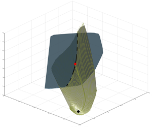
Figure 5. Visualization of the reduced-order model and the geometry of the mixed-mode SSM carrying the model flow. Panel (b) shows the mixed-mode SSM (green surface) in the  $(J,K,\Delta E)$ plane obtained as the image of the domain shown in (a) under the parametrization $\boldsymbol {W}$. The relative energy $\Delta E$ is defined as (3.6). The fixed points, the base state and the LB travelling wave are indicated with coloured dots. The dashed line denotes the predicted stable manifold of the LB travelling wave in the SSM-reduced model. The directory, including the data and the Jupyter notebook that generated this figure can be accessed at https://www.cambridge.org/S0022112023009564/JFM-Notebooks/files/Figure5/fig5.ipynb.
3.3. Capturing the edge of chaos in the reduced-order model
The mixed-mode SSM shown in figure 5(b) is two-dimensional, and the edge manifold (i.e. the stable manifold of the LB travelling wave) has codimension one. Adding up their dimensions results in  $d+1$, where $d$ is the dimension of the phase space of (2.14). Therefore, these two manifolds generically intersect transversely along a one-dimensional curve. This implies that the intersection is robust under small perturbations to system (2.5).
The generically expected transverse intersection of the SSM with the edge manifold is displayed in figure 6, where the mixed-mode SSM is the same as in figure 5 and a schematic representation of the edge manifold is added. In the three-dimensional  $(J, K, \Delta E)$ space, both the edge manifold and the mixed-mode SSM appear as two-dimensional surfaces, even though in the full phase space the edge manifold is a much higher-dimensional object.

Figure 6. Mixed-mode SSM and the edge manifold shown in the ( $J,K,\Delta E$) space. The edge manifold is sketched as a two-dimensional surface in the three-dimensional space that intersects the edge manifold along the stable manifold of the LB travelling wave in the reduced-order model (dashed black line).
From the spectrum of the LB travelling wave in figure 1, we conclude that its slowest eigenvalue with negative real part is real. Therefore, the stable manifold of this travelling wave has a one-dimensional slow SSM tangent to the eigenspace of that real eigenvalue. This SSM coincides with the stable manifold of the LB travelling wave in the reduced-order model, and hence must be the line of intersection shown in dashed lines in figure 6.
Since the intersection of the edge manifold and the mixed-mode SSM is a curve, it will not capture the dynamics within the whole edge manifold. Nevertheless, this intersection identifies a clear footprint of the edge manifold in the SSM-reduced model. To demonstrate this, we construct 10 trajectories constrained to the edge manifold using the bisection algorithm of Itano & Toh (Reference Itano and Toh2001). These trajectories converge to the LB travelling wave, which is a relative attractor within the edge. In the reduced phase space  $(J,K)$, these trajectories clearly approach the LB travelling wave along the predicted stable manifold, as shown in figure 7(a).

Figure 7. (a) Edge trajectories constructed using the bisection algorithm in the full-order model approaching the LB travelling wave displayed in the reduced-phase space. A single representative member of this ensemble of trajectories is shown with a red dashed line to guide the eye. The stable manifold of the LB travelling wave predicted from the reduced-order model is shown in black. In panel (b), trajectories of the full-order model are initialized by placing initial conditions (ICs) on both sides of the predicted edge in the reduced-order model.
The distinguishing property of the edge manifold is that it divides the phase space locally around the LB travelling wave. We show that its footprint in the reduced-order model also has this dividing role by initializing a set of trajectories in the reduced phase space at a fixed distance  $\delta =0.01$ from the stable manifold. Initial conditions are then prepared using the parametrization $\boldsymbol {W}$ and are supplied to the full-order model Openpipeflow. Figure 7(b) shows that the initial conditions prepared in this way are clearly separated in both the SSM-reduced model and the full-order model.
In figure 8(a), we show a grid of initial conditions in a rectangle around the LB travelling wave in the reduced-order model. The initial conditions for the full-order model are prepared using the identified parametrization  $\boldsymbol {W}$ and are integrated forward in time. Different colours indicate the different long-time behaviours of the grid of initial conditions. The stable manifold of the reduced-order model clearly separates the trajectories of the full-order model, as expected.

Figure 8. (a) Phase portrait of the SSM-reduced model with a grid of test trajectories. Initial conditions are placed in a grid around the LB travelling wave and are integrated forward in time using the full-order model. The initial conditions are coloured according to their long-time behaviour, as seen in the insets. The predicted edge manifold footprint is shown in black. (b) Time spent by these trajectories near the edge as a function of their initial distance from the edge measured in the SSM-reduced phase space. This time is defined as the time needed to reach a distance of  $D_{max} = 0.1$ from the LB travelling wave. A least-squares fit of the form $T=C - ({1}/{\lambda })\log \xi _0$ is also shown with $C=-234 \pm 14$ and $\lambda = 0.0175 \pm 0.0005$.
Another indication that this separation is indeed caused by the saddle-type edge state is the slowdown of trajectories, which is already present in a linear system. Consider a linear system with a saddle-type fixed point that has a one-dimensional unstable manifold. In diagonal form, the dynamics along the unstable subspace are
 \begin{equation} \dot{\xi} = \lambda \xi,\quad \text{for } \lambda > 0, \end{equation}
while for the remaining coordinates we have
 \begin{equation} \dot{\eta}_i=-\kappa_i \eta_i,\quad \text{for } \kappa_i>0,\ i=1,\ldots, d-1. \end{equation}
For sufficiently long times, the distance of a trajectory from the saddle is well approximated by its  $\xi$ coordinate component, i.e. the distance $\delta (t)$ can be written as $\delta (t)=\xi _0{\rm e}^{\lambda t}$. Therefore, the time $T$ it takes for a trajectory to leave the $\delta _{max}$-neighbourhood of the saddle satisfies $\delta _{max}=\xi _0 {\rm e}^{\lambda T}$, or, equivalently
 \begin{equation} T = \frac{1}{\lambda}\log \delta_{max} - \frac{1}{\lambda}\log \xi_0, \end{equation}
where  $\xi _0$ measures the initial distance from the stable subspace.
To demonstrate the slowdown, starting from the initial conditions shown in figure 8(a), we record the time needed for the full-order model trajectory to develop a distance of  $\delta _{max} =0.1$ from the LB travelling wave. Figure 8(b) shows the dependence of this time on the initial distance from the edge manifold in the reduced model. This relationship can be well described by a logarithmic function of the form (3.9), which would hold for a linear system. Therefore, we expect that $T=C -({1}/{\lambda })\log \xi _0$ is satisfied approximately for some constants $C$ and $\lambda$. We obtain $\lambda = 0.0175$ from a least squares fit to the data, which reasonably matches the true unstable eigenvalue of the LB travelling wave, $\lambda ^{(+)}$.
Although the one-dimensional footprint of the edge manifold cannot act as a global barrier in the phase space, it is still an influential curve for trajectories near the LB travelling wave. Since the mixed-mode SSM is constructed to be tangent to the slowest dynamics, it is locally attracting. Therefore, one may project nearby trajectories onto the mixed-mode SSM to decide their long-term dynamics: if the projection lies above the footprint of the edge manifold within the SSM, then the trajectory is expected to become turbulent. Otherwise, the trajectory is expected to quickly laminarize. As one moves away from the vicinity of the LB, this correspondence will gradually break down due to the overall complicated shape of the edge (Schneider et al. Reference Schneider, Eckhardt and Yorke2007; Mellibovsky et al. Reference Mellibovsky, Meseguer, Schneider and Eckhardt2009).
3.4. Parameter dependent SSM-reduced models
The spectrum of the LB travelling wave changes smoothly as the Reynolds number is varied, therefore the slowest mixed-mode SSM remains two-dimensional for a wide range of Reynolds numbers. As in Kaszás et al. (Reference Kaszás, Cenedese and Haller2022), we may then seek a parametrization of the Reynolds number-dependent family of mixed-mode SSMs. Similarly, the reduced dynamics on the family of manifolds then also depend on the Reynolds number. Formally, this means that we seek  $\boldsymbol {W}$ and $\boldsymbol {f}$ in a Reynolds number-dependent form
 \begin{equation} \boldsymbol{u}(r,\varphi,z) = \boldsymbol{W}(J,K, {Re}) = \boldsymbol{u}_{HP}(r) + \sum_{l=0}^{N_p}\sum_{1\leq n+m\leq M_p}\boldsymbol{w}_{nml}(r, \varphi,z)K^mJ^{n} {Re}^l \end{equation}
and
 \begin{equation}
\frac{{\rm d}}{{\rm
d}t}\begin{pmatrix}J \\ K \end{pmatrix} =
\boldsymbol{f}(J,K, {Re})= \sum_{l=0}^{N_p}\sum_{1\leq
n+m\leq M_r} \begin{pmatrix} R^{(J)}_{nml} K^m J^n \,
{Re}^l \\ R_{nml}^{(K)} K^m J^n \,
{Re}^l\end{pmatrix}. \end{equation}
\begin{equation}
\frac{{\rm d}}{{\rm
d}t}\begin{pmatrix}J \\ K \end{pmatrix} =
\boldsymbol{f}(J,K, {Re})= \sum_{l=0}^{N_p}\sum_{1\leq
n+m\leq M_r} \begin{pmatrix} R^{(J)}_{nml} K^m J^n \,
{Re}^l \\ R_{nml}^{(K)} K^m J^n \,
{Re}^l\end{pmatrix}. \end{equation}
The general dependence of these expressions on the Reynolds number is restricted by the requirement that the laminar state must be a fixed point at  $J=K=0$ for all values of the Reynolds number, therefore $\boldsymbol {w}_{00l} =0$ and $R_{00l}=0$ must hold for all $l$.
$l$.
To construct a parameter-dependent SSM-reduced model, we select the range  ${{Re}\in [2400, 2520]}$, where the slowest eigenvalues of the LB travelling wave do not change considerably and hence the mixed-mode SSMs are only expected to show minor variation. In this case, we can take a linear approximation for the Reynolds-number dependence in (3.10) and (3.11), i.e. $N_p=1$. We use three sets of training trajectories initialized at ${Re} = 2400; 2550; 2520$. These are prepared in the same way as described in the case of ${Re}=2400$. Figure 9 shows this parametrized family of reduced dynamics in the ( ${Re}, J, K$) space. We find that the phase portraits of the reduced models are qualitatively the same for all Reynolds numbers in this range.

Figure 9. Family of SSM-reduced models parametrized by the Reynolds number. Phase portraits at the sections  $Re = 2400$ and $Re = 2520$ are shown, along with the LB travelling wave and its stable and unstable manifolds computed from the SSM-reduced models.
4. Conclusion
We have constructed and tested invariant manifold-based reduced-order models for a transitional pipe flow at  $Re=2,400$. Specifically, we have computed a mixed-mode SSM, as recently defined by Haller et al. (Reference Haller, Kaszás, Liu and Axås2023), to capture the slowest dynamics characteristic of the LB travelling wave in the pipe flow. Following the numerical set-up of Willis et al. (Reference Willis, Cvitanović and Avila2013), we used a symmetry-restricted version of the dynamics, resulting in the LB travelling wave coinciding with the edge state. In addition, we used the method of slices to factor out the physically irrelevant directions for the time evolution of the trajectories. We believe that the present study is the first example of applying SSM-based reduced-order models to systems exhibiting symmetry. We have used a Python-based implementation of the data-driven SSM-reduction method, SSMLearnPy (Cenedese et al. Reference Cenedese, Kaszás and Haller2023). To make the dataset accessible, we provide it in a compressed format by performing linear dimensionality reduction first (principal component analysis) on the full dataset to reduce its size. We stress, however, that the results presented here were all obtained using the complete dataset.
The intersection of the mixed-mode SSM with the stable manifold of the edge state revealed a structurally stable curve in phase space, the slowest submanifold within the edge manifold. We have demonstrated by direct numerical simulation that the extracted curve, the one-dimensional footprint of the edge manifold, already displays edge-like characteristics: it separates laminarizing and turbulent trajectories in the phase space. This illustrates that the identified structure can be used to predict whether a given initial condition develops turbulence or simply laminarizes. We have also constructed parameter-dependent SSM-reduced models that remain valid over a range of Reynolds numbers.
For simplicity, we carried out the calculations following an additional step of symmetry reduction through the method of slices. To obtain structures in the full phase space, one simply takes the direct product of the identified structures with the group orbit of streamwise translations. For example, the mixed-mode SSM of figure 6 becomes a three-dimensional structure and its intersection with the edge manifold becomes a cylinder in the full phase space. Alternatively, using the non-sliced simulation data, one may look for the mixed-mode SSM as a three-dimensional manifold.
In this study, we utilized the small domain size and the additional shift–reflect symmetry and the two-fold azimuthal rotation symmetry restrictions. These assumptions made it possible to conclude that the edge manifold is locally of codimension one, enabling the easy characterization of its slowest submanifold as the intersection with the mixed-mode SSM. Although these assumptions fail for more general pipe flows, a similar approach could be employed even in longer pipes (Avila et al. Reference Avila, Willis and Hof2010, Reference Avila, Mellibovsky, Roland and Hof2013) without imposing the symmetries. By generating trajectories restricted to the edge of chaos using the bisection method (Itano & Toh Reference Itano and Toh2001), one could find the most influential submanifolds within the edge along with the dynamics restricted onto them. This would, however, require constructing invariant manifolds of considerably higher dimensions which brings additional challenges.
Supplementary material
Computational Notebook files are available as supplementary material at https://doi.org/10.1017/jfm.2023.956 and online at https://www.cambridge.org/S0022112023009564/JFM-Notebooks. The code and data (in compressed format) used in the paper is available in the repository https://github.com/haller-group/SSMLearnPy. The complete dataset is available from the authors upon request.
Acknowledgements
We are grateful to F. Kogelbauer, A. Willis and M. Li for several insightful conversations. The numerical simulations were performed on the Euler cluster operated by the High Performance Computing group at ETH Zürich.
Funding
We acknowledge support from the Turbulent Superstructures Program (SPP1881) of the German National Science Foundation (DFG).
Declaration of interests
The authors report no conflict of interest.
Appendix A. Resonance conditions
The mixed-mode SSM of the LB travelling wave, as constructed by Haller et al. (Reference Haller, Kaszás, Liu and Axås2023), exists under the conditions of the linearization theorem of Sternberg (Reference Sternberg1958). These require that the eigenvalues of the Jacobian of (2.5) at the LB travelling wave be non-resonant. Specifically, denoting the eigenvalues as  $\lambda _i$ and ordering them according to descending real part, we require
 \begin{equation} \lambda_j \neq \sum_{i=1}^d m_i \lambda_i, \quad m_i\in \mathbb{N} \quad \sum_{i=1}^d m_i\geq2. \end{equation}
We check that the conditions (A1) hold for a finite subset of the spectrum of the LB travelling wave by constructing all admissible integer linear combinations of the leading  $23$ eigenvalues shown in figure 10(b). To select the eigenvalues nearest to resonance, for every eigenvalue $\lambda _j$, we define
 \begin{equation} D(\lambda_j) = \min_{m_i} \left \vert\lambda_j - \sum_{i=1}^d m_i\lambda_i \right \vert, \end{equation}
which measures how close  $\lambda _j$ is to being resonant. We plot the relative measure of resonance-closeness, $D(\lambda )/|\lambda |$ for the leading eigenvalues in figure 10(a). Although no exact resonance is seen in the spectrum, near-resonances of up to $0.1\,\%$ coincidence can be seen. The nearest resonance is highlighted in figure 10 as $\lambda _{20}$, whose value is
 \begin{equation} \lambda_{20}=-0.06529 + 0.00829{\rm i}. \end{equation}
With a linear combination of  $\lambda _1$, $\lambda _4$, and $\lambda _8$, we get
 \begin{equation} \lambda_{1}+\lambda_4 + 3\lambda_8=-0.06514 + 0.00822{\rm i}, \end{equation}
which yields  $D(\lambda )/|\lambda |\approx 0.2\,\%$. Although close resonances of similar severity may occur in the rest of the spectrum, we see no indication of exact resonances, hence the results of Haller et al. (Reference Haller, Kaszás, Liu and Axås2023) should apply.

Figure 10. (a) Leading eigenvalues of the LB travelling wave restricted to the  $\mathcal {S}-$invariant subspace. (b) Relative measure of resonance-closeness, $D(\lambda )/|\lambda |$ as a function of $|\lambda |$. The eigenvalue closest to being resonant, $\lambda _{20}$, is marked with a red point. The three eigenvalues generating this close resonance, $\lambda _1$, $\lambda _4$ and $\lambda _8$ are marked with orange points. The directory, including the data and the Jupyter notebook that generated this figure can be accessed at https://www.cambridge.org/S0022112023009564/JFM-Notebooks/files/Figure10/fig10.ipynb.


 Open access