


1. Introduction
The theory of the moving contact line at small capillary numbers was founded by Voinov (Reference Voinov1976) and generalized to arbitrary viscosity ratios  $M$ by Cox (Reference Cox1986). The problem is that if the no-slip boundary condition were to apply down to arbitrarily small scales (Huh & Scriven Reference Huh and Scriven1971; Bonn et al. Reference Bonn, Eggers, Indekeu, Meunier and Rolley2009; Snoeijer & Andreotti Reference Snoeijer and Andreotti2013), a contact line would not be able to move. Therefore, one needs to invoke a small length scale on which the conventional equations for fluid motion are relaxed. The simplest, and often physically realistic, such choice is the introduction of a Navier slip length $\lambda$ (Lauga, Brenner & Stone Reference Lauga, Brenner, Stone, Tropea, Foss and Yarin2008), over which a fluid may slip past a solid interface. Thus we will always assume that, as the wall is approached, the tangential velocity relative to the wall is $\lambda$ times the shear rate. The slip length is generally of the order of a few nanometres, but increases somewhat for hydrophobic surfaces (Barrat & Bocquet Reference Barrat and Bocquet1999; Cottin-Bizonne et al. Reference Cottin-Bizonne, Cross, Steinberger and Charlaix2005). A slip length is used very widely in contact line problems (Bonn et al. Reference Bonn, Eggers, Indekeu, Meunier and Rolley2009; Snoeijer & Andreotti Reference Snoeijer and Andreotti2013; Vandre, Carvalho & Kumar Reference Vandre, Carvalho and Kumar2014; Sprittles Reference Sprittles2015) in order to regularize the local flow and to thus allow contact line motion, but is usually not important elsewhere in the flow. The inner length scale $\lambda$ is contrasted with an outer ‘macroscopic’ length scale $R$, for example the radius of a spreading drop or the capillary length scale in the problem.
Cox (Reference Cox1986) clarified the structure of low capillary number problems in terms of the ratio  $\epsilon = \epsilon _0\lambda / R$ between the two length scales; $\epsilon _0$ is a numerical factor to be determined. From a general analysis, Cox (Reference Cox1986) obtained (see also Sibley, Nold & Kalliadasis Reference Sibley, Nold and Kalliadasis2015)
 \begin{equation} g(\theta_{eq}) = g(\theta_{app}) + {Ca}\,\ln\epsilon, \end{equation}
where
 \begin{equation} g(\theta) = \int_0^{\theta}\frac{u - \cos u\sin u}{2\sin u}\,\textrm{d}u, \end{equation}
 for a single phase (a liquid volume, neglecting the effect of a surrounding gas). Here,  $\theta _{eq}$ is the (equilibrium) contact angle on the microscopic scale, and $\theta _{app}$ is the apparent contact angle. In the case of a small spreading drop, this is the angle a spherical cap, fitted to the drop, makes with the solid. In Cox's analysis, the dimensionless capillary number
 \begin{equation} {Ca} = \frac{U\eta}{\gamma} \end{equation}
is assumed small, where  $U$ is the speed of the contact line. Here, $\eta$ is the fluid viscosity, and $\gamma$ is the surface tension. For steady flow, it is often more convenient to instead think of the contact line being stationary and the wall to be moving at speed $U$, because we can then think of the interface as time independent.
In the present paper, we take the approach proposed by Snoeijer (Reference Snoeijer2006) and Chan et al. (Reference Chan, Srivastava, Marchand, Andreotti, Biferale, Toschi and Snoeijer2013), who describe the interface shape as an evolution equation for the local slope  $\theta$. For simplicity, we neglect external forcing (such as gravity), which only becomes important on a macroscopic scale. The requirement that the interface (described by its thickness $h(s)$), is assumed steady, while the substrate is moving at speed $U$ to the right, then leads to the ‘generalized lubrication’ (GL) equation. One obtains (Snoeijer Reference Snoeijer2006)
 \begin{equation} \frac{\textrm{d}^{2}\theta}{\textrm{d}s^{2}} = \frac{3{Ca}\, F(\theta,M)}{h^{2}}, \end{equation}
where  $s$ is the arclength along the interface, and
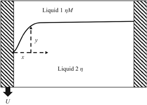
  $M=\eta _g/\eta _{l}$ the ratio of the viscosity of the outer phase (for example a gas), and the viscosity of the liquid (cf. figure 1). In the case of a single (liquid) phase only,
 \begin{equation} F(\theta) \equiv F(\theta,0) = -\frac{2\sin^{3}\theta}{3(\theta - \sin\theta\cos\theta)}. \end{equation}
Here,  $F(\theta )$ is related to $g(\theta )$ by $F(\theta )=(2/3)g(\theta )\sin ^{2}{\theta }$. The full expression $F(\theta,M)$ for two fluids is given in (2.13). To close (1.4), one has to simultaneously solve the geometrical relations
 \begin{equation} \frac{\textrm{d}h}{\textrm{d}s} = \sin\theta, \quad \frac{\textrm{d}x}{\textrm{d}s} = \cos\theta, \end{equation}
to find the interface shape  $h(x)$ in a Cartesian coordinate system. Integrating (1.4), making use of the limit of small ${Ca}$, (1.6) leads precisely to the structure given by (1.1).
Sketch of geometry; the volume of integration is shown as the dotted line.

In contrast to the approach of asymptotic matching between micro and macroscales adopted by Cox (Reference Cox1986) or Hocking & Rivers (Reference Hocking and Rivers1982), the GL equation (1.4), for small  $Ca$, gives a full representation of the interfacial profile, given that boundary conditions at the contact line and the far field are properly imposed, for arbitrary contact angles and viscosity ratios. On the large scale, boundary conditions may be the requirement for the interface to assume a drop shape, or to asymptote to a flat interface, as we will require below in our numerical tests of the equation.
The unknown length scale  $\epsilon$ appearing in Reference CoxCox's (Reference Cox1986) theory is now no longer required, but should in principle come out of the solution of (1.4). However, the slip effect is not properly implemented in (1.4) and as a result, the equation does not have solutions corresponding to a moving contact line. To account for this, Chan et al. (Reference Chan, Srivastava, Marchand, Andreotti, Biferale, Toschi and Snoeijer2013), motivated by the form of the lubrication equation, introduced the modified GL equation to yield
 \begin{equation} \frac{\textrm{d}^{2}\theta}{\textrm{d}s^{2}} = \frac{3 {Ca}\, F(\theta,M)}{h(h + c\lambda)}, \end{equation}
where  $c$ is a constant to be chosen such that the solution matches properly with the slip region. In Chan et al. (Reference Chan, Srivastava, Marchand, Andreotti, Biferale, Toschi and Snoeijer2013), in the absence of any theory for how $c$ should be chosen, this was done assuming that $c = 3$, which is true only for small angles and for a single phase (Hocking Reference Hocking1983). Here, we calculate the dependence of $c$ on the microscopic contact angle $\theta _{eq}$ and on the viscosity ratio $M$. Once $c$ is known, one can integrate (1.7) from the contact line to whichever macroscopic configuration is required for the problem.
Let us start by sketching the structure of the analysis to compute  $c$. For small ${Ca}$, it is sufficient to consider a linear perturbation of the free surface shape around a wedge with microscopic (equilibrium, for simplicity and without loss of generality) angle $\theta _{eq}$. Therefore we set $\theta =\theta _{eq}-\varphi (s)$, and, to linear order in $\varphi$, all calculations can be performed assuming a wedge geometry $h = s\sin \theta _{eq}$ for the flow (cf. figure 1). Linearizing (1.7) in $\varphi$ and integrating twice, we have
 \[ \varphi = \frac{3 {Ca}\, F(\theta_{eq},M)}{\sin^{2}\theta_{eq}} \left[\frac{h}{c\lambda} \left(\ln(h+c\lambda)-\ln h\right) +\ln(h+c\lambda) -1 \right] + Ch + C_1. \]
We are interested in solutions which only grow logarithmically, corresponding to vanishing curvature at infinity, and so  $C=0$. From the boundary condition $\varphi (0)=0$ it follows that $C_1 = 3{Ca}\,F(\theta _{eq},M)(1 - \ln c\lambda )/\sin ^{2}\theta _{eq}$, and so to leading order as $s/\lambda \rightarrow \infty$ we have
 \begin{equation} \varphi(s) = \frac{3 {Ca}\, F(\theta_{eq},M)}{\sin^{2}\theta_{eq}} \ln\frac{se\sin\theta_{eq}}{c\lambda}. \end{equation}
 Here, we calculate  $c$ for arbitrary angles $\theta _{eq}$ and arbitrary viscosity ratios $M$, based on earlier work by Hocking (Reference Hocking1977), who calculates the stress on a slip wall, assuming a straight interface $h = s\sin \theta _{eq}$. Using the fact that in the absence of inertia (Stokes dynamics), the total force on any fluid volume vanishes, we can convert the wall force to a force on the interface, which leads to bending of the interface, allowing us to determine $c$. In addition, one may also allow for an arbitrary ratio of slip lengths $\lambda _1/\lambda _2$ at the two fluid–solid interfaces, but no explicit results are available for this case. So in the interest of simplicity, we will always assume $\lambda _1 = \lambda _2 \equiv \lambda$.
2. Determining c from a force balance
2.1. A single phase
We start the analysis by considering the case of a single phase (the liquid, as shown in figure 1), which enables us to show some of the calculations in greater detail. The idea is to consider a force balance over the volume shown in figure 1, within which the Stokes equation  ${{\boldsymbol {\nabla }}}\boldsymbol {\cdot }\boldsymbol {\sigma }=0$ is satisfied; $\boldsymbol {\sigma }$ is the stress tensor. This is motivated by Reference HockingHocking's (Reference Hocking1977) calculation of the force exerted by a moving contact line on a solid boundary. Using Gauss’ theorem, and only considering the force in the $x$-direction, we obtain
 \begin{equation} \int_S \boldsymbol{n}\boldsymbol{\cdot}\boldsymbol{\sigma}\boldsymbol{\cdot}\boldsymbol{e}_x = 0, \end{equation}
where  $\boldsymbol {n}$ is the outward normal, and $S = S_i + S_c + S_w$. The volume is the slice of radius $s$ inside the fluid, where $S_i$ is the fluid–gas interface, $S_c$ a circular arc of radius $s$ inside the fluid and $S_w$ the wall, see figure 1.
The force on  $V$ coming from the interface is
 \begin{equation} \int_{S_i} \boldsymbol{n}\boldsymbol{\cdot}\boldsymbol{\sigma}\boldsymbol{\cdot}\boldsymbol{e}_x\,\textrm{d}s = -\gamma\int_{S_1} \kappa\boldsymbol{n}\boldsymbol{\cdot}\boldsymbol{e}_x\,\textrm{d}s \simeq \gamma\sin\theta_{{eq}} \int_0^{s} \frac{\textrm{d}\varphi}{\textrm{d}s}\,\textrm{d}s = \gamma\sin\theta_{{eq}} \varphi(s). \end{equation}
Here, we have used the stress boundary condition (Landau & Lifshitz Reference Landau and Lifshitz1984)  $\boldsymbol {n}\boldsymbol {\cdot }\boldsymbol {\sigma } = -\gamma \boldsymbol {n}\kappa$, where $\kappa = \textrm {d}\varphi /\textrm {d}s$ is the interface curvature and $\boldsymbol {n}\boldsymbol {\cdot }\boldsymbol {e}_x \simeq -\sin {\theta _{{eq}}}$. The integral over $S_w$, representing the total force $w$ on the wall between the origin and $x=s$, has been calculated by Hocking (Reference Hocking1977) for Stokes flow in a corner with slip at the wall, and a free-slip condition at the interface. The contribution $v$ of the force on $S_c$ can be inferred from the far-field limit of the flow, calculated by Huh & Scriven (Reference Huh and Scriven1971). Thus (2.1) gives
 \begin{equation} \gamma\sin\theta_{{eq}} \varphi(s) = -v - w, \end{equation}
which we compare to (1.8) to find  $c$.
$c$.
To find  $v$ and $w$, we need to consider the flow in the wedge-shaped fluid domain (cf. figure 1) of opening angle $\theta =\theta _{{eq}}$. In Hocking (Reference Hocking1977), the flow is solved subject to the slip boundary condition (with $u$ the horizontal component of the velocity)
 \[ u(x,0) = U + \lambda\frac{\partial u}{\partial y}, \]
on the wall. It is convenient to count the angle  $\phi$ from the interface; the velocity field is given in terms of the streamfunction
 \[ u_r = \frac{1}{r}\frac{\partial \psi}{\partial \phi}, \quad u_{\phi} = -\frac{\partial \psi}{\partial r}. \]
The boundary conditions on both boundaries are zero normal velocity, and vanishing shear stress  $\sigma _{r\phi }=0$ on the interface. Thus for $\phi = \theta _{{eq}}$ (the wall) we have
 \[ \frac{\partial \psi}{\partial r} = 0, \quad U = \frac{1}{r}\frac{\partial \psi}{\partial \phi} + \frac{\lambda}{r^{2}}\frac{\partial^{2} \psi}{\partial \phi^{2}}, \]
and for  $\phi =0$ (the interface)
 \[ \frac{\partial \psi}{\partial r} = 0, \quad \frac{1}{r^{2}}\frac{\partial^{2} \psi}{\partial \phi^{2}} - \frac{\partial^{2} \psi}{\partial r^{2}} + \frac{1}{r}\frac{\partial \psi}{\partial r} = 0. \]
In the limit  $r\gg \lambda$ we can neglect the effects of slip, and we should fall back on the similarity solution $\psi = r f(\theta _{{eq}})$ found by Huh & Scriven (Reference Huh and Scriven1971). With the ansatz
 \begin{equation} f = a_1\sin\phi + a_2\cos\phi + a_3\phi\sin\phi + a_4\phi\cos\phi, \end{equation}
the boundary conditions are
 \[ f(0) = 0, \quad f''(0) = 0, \quad f(\theta_{{eq}}) = 0, \quad f'(\theta_{{eq}}) = U. \]
The coefficients are ( $D = \theta _{{eq}} - \sin \theta _{{eq}}\cos \theta _{{eq}}$),
 \[ a_1 = -\frac{U\theta_{{eq}}\cos\theta_{{eq}}}{D}, \quad a_2 = 0,\quad a_3 = 0, \quad a_4 = -\frac{U\sin\theta_{{eq}}}{D}, \]
and so the stresses become
 \begin{equation} \sigma_{rr} = \frac{2\eta U}{rD}\sin\theta_{{eq}}\cos\phi,\quad \sigma_{r\phi} = \frac{2\eta U}{rD}\sin\theta_{{eq}}\sin\phi. \end{equation}
Using (2.5a,b) and
 \[ \boldsymbol{n}\boldsymbol{\cdot}\boldsymbol{\sigma}\boldsymbol{\cdot}\boldsymbol{e}_x = \sigma_{rr}\cos(\theta_{{eq}}-\phi) + \sigma_{r\phi}\sin(\theta_{{eq}}-\phi), \]
we find
 \[ v = \int_{S_c} \boldsymbol{n}\boldsymbol{\cdot}\boldsymbol{\sigma}\boldsymbol{\cdot}\boldsymbol{e}_x\,\textrm{d}s = r\int_0^{\theta_{{eq}}} \boldsymbol{n}\boldsymbol{\cdot}\boldsymbol{\sigma}\boldsymbol{\cdot}\boldsymbol{e}_x\,\textrm{d}\phi = -\frac{3\eta UF(\theta_{{eq}})}{\sin\theta_{{eq}}}, \]
where  $F(\theta _{{eq}})$ is the angle dependence from the GL model given previously in (1.5). As an aside, $F(\theta _{{eq}})$ can easily be calculated from $\sigma _{\phi \phi }$, evaluated at the interface $\phi =0$, and using the stress boundary condition $\gamma \kappa = -\sigma _{\phi \phi }|_{\phi =0}$. On the other hand, using $h=s\sin \theta _{{eq}}$ and integrating (1.4) once, we have
 \begin{equation} \kappa = \frac{\textrm{d}\varphi}{\textrm{d}s} = \frac{3{Ca}\,F(\theta_{{eq}})}{s\sin^{2}\theta_{{eq}}}, \end{equation}
comparing with  $\sigma _{\phi\phi}|_{\phi =0}$ yields $F(\theta _{{eq}})$.
Finally, Hocking (Reference Hocking1977) has calculated the force on the wall
 \[ w = \int_{S_w} \boldsymbol{n}\boldsymbol{\cdot}\boldsymbol{\sigma}\boldsymbol{\cdot}\boldsymbol{e}_x\,\textrm{d}s = -\int_{S_w} \sigma_{xy}\,\textrm{d}s = U\eta\left[-\frac{3F(\theta_{{eq}})} {\sin\theta_{{eq}}}\ln\frac{s}{\lambda} + h_1\right], \]
where  $h_1(\theta _{{eq}})$ is the solution of an integral equation, which in general has to be solved numerically. Using (2.3), it follows that, in the general case,
 \[ \varphi(s) = {Ca}\,\left[ \frac{3 F(\theta_{{eq}})}{\sin^{2}\theta_{{eq}}}\ln\frac{se}{\lambda} - \frac{h_1}{\sin\theta_{{eq}}}\right], \]
which is precisely of the expected form (1.8). Comparing the two, we find
 \begin{equation} c = \sin\theta_{{eq}} \exp\left(\frac{\sin\theta_{{eq}} h_1(\theta_{{eq}})}{3 F(\theta_{{eq}})}\right), \end{equation}
which is our main result in the case of a single phase.
The function  $c(\theta _{{eq}})$ as obtained from (2.7) is shown in figure 2. To compute $h_1(\theta _{{eq}})$, we have solved the integral equation (3.6) of Hocking (Reference Hocking1977) numerically using a relatively simple iterative procedure. The red cross is the exact value $h_1({\rm \pi} /2) = 4(\gamma _E-\ln 2)/{\rm \pi}$, giving
 \begin{equation} c({\rm \pi}/2) = \exp({\ln 2-\gamma_E}) \approx 1.12. \end{equation}
For small values of  $\theta _{{eq}}$, Reference HockingHocking's (Reference Hocking1977) asymptotic argument leads to $h_1=-\hat {k}\ln {\hat {k}}$, where $\hat {k}=-3F(\theta _{{eq}})/\sin {\theta _{{eq}}}$. However, in order to obtain a consistent expansion, $\hat {k}$ had to be expanded to the next order beyond (3.18) of (Hocking Reference Hocking1977), which results in
 \begin{equation} c =3-(9/10)\theta_{{eq}}^{2}. \end{equation}
For  $\theta _{{eq}}=0$, one of course recovers $c = 3$, as known from lubrication theory.
The  $c$-factor as a function of $\theta _{{eq}}/{\rm \pi}$ for $M=0$, calculated numerically by evaluating the integral expressions for $h_1$ as given by Hocking (Reference Hocking1977). The (red) dashed lines are the asymptotic expansions (2.9) and (2.10) for small $\theta _{{eq}}$ and as $\theta _{{eq}} \to {\rm \pi}$, respectively. The (red) cross marks the analytical value $c({\rm \pi} /2) = \exp ({\ln 2-\gamma _E})$ (see (2.8)).

On the other hand for  $\theta _{{eq}}\to {\rm \pi}$, using Reference HockingHocking's (Reference Hocking1977) leading-order expression for $h_1$, we obtain
 \begin{equation} c= ({\rm \pi}-\theta_{{eq}})\exp{\left[-{\rm \pi}/({\rm \pi}-\theta_{{eq}})\right]}. \end{equation}
The limits (2.9) and (2.10) are shown in figure 2 as the red dashed lines, and are seen to agree very well with our numerical solution. Interestingly,  $c$ becomes very small for angles close to ${\rm \pi}$. For example, $c(0.9 {\rm \pi}) = 1.04\cdot 10^{-4}$, showing that in general $c$ cannot be inferred from a comparison with lubrication theory.
2.2. Two phases
We now generalize to the case of two phases (arbitrary viscosity ratio  $M$), for which the constant $c$ has never been calculated, not even for small angles. We explain the general structure, but explicit results are available for $\theta _{{eq}}={\rm \pi} /2$ only.
In contrast to the previous subsection, we now have the integral (2.1) over the surface of two volumes  $V_1$ and $V_2$; $V_1$ is the volume over the ‘liquid’ phase as before (labelled 1), $V_2$ is the corresponding slice of the same radius $s$ over phase 2 (the ‘gas’). Then (2.1), written for each phase, becomes
 \begin{equation} \int_{S_i} \boldsymbol{n}\boldsymbol{\cdot}\boldsymbol{\sigma}_1\boldsymbol{\cdot}\boldsymbol{e}_x + v_1 + w_1 = 0, \quad -\int_{S_i} \boldsymbol{n}\boldsymbol{\cdot}\boldsymbol{\sigma}_2\boldsymbol{\cdot}\boldsymbol{e}_x + v_2 + w_2 = 0, \end{equation}
where  $v$ and $w$ have the same meanings as before, but for each phase separately. Using the stress condition $\boldsymbol {n}\boldsymbol {\cdot }(\boldsymbol {\sigma }_1-\boldsymbol {\sigma }_2) = -\gamma \boldsymbol {n}\kappa$, this yields
 \begin{equation} \gamma\sin\theta_{{eq}} \varphi(s) = -v_1 - v_2 - w_1 - w_2. \end{equation}
 The solution for a no-slip flow, for general  $M$, has been given by Huh & Scriven (Reference Huh and Scriven1971). At the interface between the two fluids we now have continuity of the tangential velocity (the normal velocity vanishes), and of shear stress. If the streamfunctions in either phase are $\psi _{1/2} = r f_{1/2}(\theta _{{eq}})$, the boundary conditions are
 \begin{gather*} f_1(0) = f_2(0) = 0, \quad f_1''(0) = M f_2''(0), \quad f_1'(0) = f_2'(0), \quad f_1(\theta_{{eq}}) = 0, \\ f_1'(\theta_{{eq}}) = U, \quad f_2(\theta_{{eq}}-{\rm \pi}) = 0, \quad f_2'(\theta_{{eq}}-{\rm \pi}) = -U. \end{gather*}
The results are a little too complicated to write out here, but as in (2.6), we can calculate the general form of  $F(\theta,M)$ in (1.4), by computing the normal stress on the interface from either phase, giving
 \[ \left.\sigma^{(2)}_{\phi\phi}\right|_{\phi=0} - \left.\sigma^{(1)}_{\phi\phi}\right|_{\phi=0} = \gamma\kappa = \frac{3U\eta}{r\sin^{2}\theta_{{eq}}} F(\theta_{{eq}},M). \]
Comparison with (1.4) then shows that
 \begin{equation} F(\theta,M) = -\frac{2\sin^{3}\theta}{3}\frac{M^{2}F_1(\theta) + 2MF_3(\theta) + F_1({\rm \pi}-\theta)}{MF_1(\theta)F_2({\rm \pi}-\theta) + F_1({\rm \pi}-\theta)F_2(\theta)}, \end{equation}
where
 \[ F_1 = \theta^{2}-\sin^{2}\theta, \quad F_2 = \theta - \sin\theta\cos\theta, \quad F_3 = \theta({\rm \pi}-\theta) + \sin^{2}\theta; \]
note the sign error in Chan et al. (Reference Chan, Srivastava, Marchand, Andreotti, Biferale, Toschi and Snoeijer2013).
Furthermore, it follows from the Huh–Scriven solution, after a lengthy but elementary calculation, that
 \[ v_1 + v_2 = -\frac{3U\eta F(\theta_{{eq}},M)}{\sin\theta_{{eq}}}. \]
The shear force on the wall now has contributions from both phases, and it follows from Hocking (Reference Hocking1977) that
 \[ w_1 + w_2 = U\eta\left[-\frac{F(\theta_{{eq}},M)}{\sin\theta_{{eq}}} \ln\frac{s}{\lambda} + h_1 + M h_2\right]. \]
Taken together with (2.12), this yields the interface deformation
 \[ \varphi(s) = {Ca}\,\left[ \frac{3 F(\theta_{{eq}},M)}{\sin^{2}\theta_{{eq}}} \ln\frac{se}{\lambda} - \frac{h_1 + M h_2}{\sin\theta_{{eq}}}\right], \]
and comparing with (1.8)
 \begin{equation} c = \sin\theta_{{eq}} \exp\left(\frac{\sin\theta_{{eq}} (h_1+M h_2)}{3 F(\theta_{{eq}},M)}\right), \end{equation}
now involving two numerical constants  $h_1$ and $h_2$. This completes our calculation, but it remains to calculate the constants $h_1$ and $h_2$, which are functions of $\theta _{{eq}}$ and $M$. According to Hocking (Reference Hocking1977) this can be done explicitly for a right angle $\theta _{{eq}} = {\rm \pi}/2$, for which
 \begin{equation} h_1 = \frac{(1-M)h_a+2Mh_b}{1+M}, \quad h_2 = \frac{-(1-M)h_a+2Mh_b}{1+M}, \end{equation}
where  $h_a = (4/{\rm \pi} )(\gamma _E - \ln 2)$ and $h_b = -1.539$. The geometrical factor is
 \begin{equation} F({\rm \pi}/2,M)=-\frac{4}{3{\rm \pi}} \frac{(M+1)^{2}{\rm \pi}^{2}-4(M-1)^{2}}{({\rm \pi}^{2}-4)(M+1)}, \end{equation}
for right angles. It is now a simple matter to compute the  $c$-factor, shown in figure 3, as a function of $\log _{10}M$. For small $M$ (to the left of the figure), one recovers (2.8). For large $M$, on the other hand, $c$ rises significantly towards $c \to \exp (-{\rm \pi} (h_a+2h_b)/4) \approx 12.60$ as $M\to \infty$, showing once more that the behaviour for finite angles is significantly different from the lubrication result.
The  $c$-factor as a function of $\log _{10}M$ for $\theta _{{eq}} = {\rm \pi}/2$. Horizontal (red) dashed lines are the asymptotes of $c$ for $M= 0$ ( $c\approx 1.12$) and $M\to \infty$ ( $c\approx 12.60$).

3. Discussion
To illustrate and validate our results, we consider a plate being pushed steadily into a container of fluid 2, with an outer fluid 1, as shown in figure 4(a). This is the classical dip-coating configuration, used industrially to coat a solid with liquid, and studied in many experiments (Blake & Ruschak Reference Blake and Ruschak1979; Benkreira & Khan Reference Benkreira and Khan2008; Benkreira & Ikin Reference Benkreira and Ikin2010; Marchand et al. Reference Marchand, Chan, Snoeijer and Andreotti2012; Vandre, Carvalho & Kumar Reference Vandre, Carvalho and Kumar2012; Vandre et al. Reference Vandre, Carvalho and Kumar2014). To account for the effect of gravity, in units of the capillary length  $l_{\gamma }$ (Snoeijer & Andreotti Reference Snoeijer and Andreotti2013), one has to add a term $-\cos (\theta )$ to the modified GL equation (1.7) (Chan et al. Reference Chan, Srivastava, Marchand, Andreotti, Biferale, Toschi and Snoeijer2013). One of the main aims is to calculate the apparent contact angle as well as the critical capillary number at which fluid 1 is entrained into fluid 2. As shown in Kamal etal. (Reference Kamal, Sprittles, Snoeijer and Eggers2018), for small values of $M$ (for example when fluid 1 is air), the critical capillary number is so high that it cannot be calculated within an expansion for small ${Ca}$. However, here we focus on the regime of smaller ${Ca}$ up to 0.1, and compute the apparent contact angle, to assess the improvement of our predictions over Chan et al. (Reference Chan, Srivastava, Marchand, Andreotti, Biferale, Toschi and Snoeijer2013), where the results it was assumed that $c=3$. $(a)$ Sketch of the interface shape between two liquids produced by a descending plate; all lengths are in units of the capillary length scale $l_{\gamma }$. ( $b$,
$b$, $c$) Comparison of interface profiles from FEM with GL simulations for (i) the correct value of $c({\rm \pi} /2,M)$ and (ii) the previously used value $c(0,M=0)=3$ for ${Ca}=0.1,\ M=0$ and ${Ca}=0.01,\ M=1$, respectively. Left plots: steady profiles, right plots: relative error of the GL profile $y_{{GL}}$ compared to FEM profile $y_{{FEM}}$. Both the GL and FEM simulations are performed for a slip length $\lambda =0.0001$.

We compare full numerical simulations of the dip-coating problem, using the finite elements method (FEM) described in detail in Kamal et al. (Reference Kamal, Sprittles, Snoeijer and Eggers2018), and based on a framework benchmarked in Sprittles (Reference Sprittles2015), with results of the GL equation for  ${Ca}$ up to 0.1. We show an example with $M=0$ and one with $M=1$, with a contact angle of ${\rm \pi} /2$ (figure 4( $b$,
$b$, $c$), respectively). On the left, the solid line is the interface profile found from FEM, the red dashed line comes from integrating (1.7) using the new expression of $c$ in (2.7), as obtained by the present theory; very good agreement is found.
To demonstrate the importance of using the correct value of  $c$ in order to obtain this agreement, we also plot the profile obtained using the value $c=3$, proposed previously (Snoeijer Reference Snoeijer2006; Chan et al. Reference Chan, Srivastava, Marchand, Andreotti, Biferale, Toschi and Snoeijer2013). However, this value is only appropriate in the limit of small contact angles and no outer fluid ( $M=0$). As a result, the dot-dashed blue, which is the profile thus obtained from the ‘old’ GL equation, differs significantly from the ‘exact’ result, obtained from direct numerical simulation, including poorly predicting the (macroscopic) height far away from the contact line.
To focus on the solutions very close to the contact line, we also plot the relative deviation between the FEM simulation and solutions obtained from integrating (1.7) on the right of figure 4. For the solid line we use the correct value of  $c$, the dashed line represents the value $c=3$. For the smaller capillary number, using the $c$-value as calculated in the present paper, the deviation is negligible, and even for a capillary number ${Ca} = 0.1$, the relative error remains small; when the capillary number becomes of order unity the GL equation fails (Kamal et al. Reference Kamal, Sprittles, Snoeijer and Eggers2018), since it is an expansion for small ${Ca}$ only. On the other hand for $c=3$ the relative error is significant in both cases as one approaches the contact line.
Having benchmarked the new theory against FEM calculations, in order to assess the improvement of the current theory over the previous GL theory using  $c=3$, we compare the apparent contact angle $\theta _{{app}}$ in both cases, for a wide range of parameters $M$ and $\theta _{{eq}}$. For the dip-coating geometry shown in figure 4, $\theta _{{app}}$ can be calculated by comparing the depth $\Delta$ of the contact line relative to the level of the bath to the depression of a static meniscus (Landau & Lifshitz Reference Landau and Lifshitz1984) $\Delta =\sqrt {2(1-\sin {\theta _{{app}}})}$ (once more in units of $l_{\gamma }$).
We use the GL equation to evaluate the error in predictions of  $\theta _{{app}}$ between simulations where the correct value of $c$ is implemented, to those where the lubrication value ( $c=3$) is used (figure 5). For finite viscosity ratios $M$, above a critical capillary number ${Ca}_{{cr}}$ the stationary meniscus bifurcates to a time-dependent solution, in which the outer fluid is entrained (Snoeijer & Andreotti Reference Snoeijer and Andreotti2013; Kamal et al. Reference Kamal, Sprittles, Snoeijer and Eggers2018). In figure 5(a), we vary the viscosity ratio $M$ as the contact angle is held constant at $\theta _{{eq} }= {\rm \pi}/2$. It shows the considerable error in $\theta _{{app}}$, which increases rapidly as ${Ca}_{{cr}}$ is approached. In figure 5(b), we hold $M=0$ constant, while varying $\theta _{{eq} }$ between ${\rm \pi} /2$ and ${\rm \pi}$. As expected, the error in $\theta _{{app}}$ increases substantially as $\theta _{{eq}}$ increases. In fact, as seen in (2.10), the true value of $c$ decreases exponentially as $\theta _{{eq}}={\rm \pi}$ is approached.
Comparing the error between predictions of the apparent contact angle  $\theta _{{app}}$ between $c(\theta _{eq},M)$ and $c=3$. $(a)$ The error as a function of $Ca$ comparing different viscosity ratio $M$ and fixed equilibrium contact angle $\theta _{{eq}}= {\rm \pi}/2$, $(b)$ the error as a function of $Ca$ comparing different $\theta _{{eq}}$ and fixed viscosity ratio $M=0$. $(a)$ for $M=0,\ 1$ and $10$,
$10$,  $c({\rm \pi} /2,M)=1.12,\ 2.05$ and $6.40$, respectively. Dotted horizontal lines mark the position of the bifurcation point $Ca_{{cr}}$ predicted from the GL model. $(b)$ For $\theta _{{eq}}=0.5{\rm \pi},\ 0.6{\rm \pi},\ 0.7{\rm \pi}$ and $0.8{\rm \pi}$, $c(\theta _{{eq}},M=0)=1.12,\ 0.60,\ 0.22$ and $0.030$, respectively. Simulations are performed in the GL model for a slip length $\lambda =0.0001$.

In conclusion, we have analysed the Cox–Voinov theory with slip, for arbitrary contact angles and arbitrary viscosity ratios. Closed form expressions are provided using the generalized lubrication equation, which is shown to be a powerful tool to calculate interface flows involving moving contact lines in situations in which the interface slope is not necessarily small. The present paper provides a consistent version of the GL equation for arbitrary contact angles.
Acknowledgements
This work has been financially supported by the Engineering and Physical Sciences Research Council (grants EP/N016602/1, EP/S029966/1 and EP/P031684/1). T.S.C. gratefully acknowledges financial support from the UiO: Life Science initiative at the University of Oslo. J.E. acknowledges the support of Leverhulme Trust International Academic Fellowship IAF-2017-010.
Declaration of interests
The authors report no conflict of interest.


 Open access